The Incidence and Cross Methods for Efficient Radar Detection

Abstract

The designation of the radar system is to detect the position and velocity of targets around us. The radar transmits a waveform, which is reflected back from the targets, and echo waveform is received. In a commonly used model, the echo is a sum of a superposition of several delay-Doppler shifts of the transmitted waveform, and a noise component. The delay and Doppler parameters encode, respectively, the distances, and relative velocities, between the targets and the radar. Using standard digital-to-analog and sampling techniques, the estimation task of the delay-Doppler parameters, which involves waveforms, is reduced to a problem for complex sequences of finite length $N.$ In these notes we introduce the Incidence and Cross methods for radar detection. One of their advantages, is robustness to inhomogeneous radar scene, i.e., for sensing small targets in the vicinity of large objects. The arithmetic complexity of the incidence and cross methods is $O(N\log N+r^{3})$ and $O(N\log N+r^{2}),$ for $r$ targets, respectively. In the case of noisy environment, these are the fastest radar detection techniques. Both methods employ chirp sequences, which are commonly used by radar systems, and hence are attractive for real world applications.

I Introduction

The radar system provides detection of the position and velocity of moving targets. The radar transmits—see Figure 1 for illustration—an analog waveform $S_{A}(t),$ $t\in\mathbb{R},$ of bandwidth $W$. While the actual waveform is modulated onto a carrier frequency $f_{c}\gg W,$ we consider a widely used complex baseband model for the multi-target channel (see Section I.A. in [1] and references therein). In addition, we make the sparsity assumption on the finiteness of the number of targets. The waveform $S_{A}$ hits the targets, and the analog waveform received as echo is given by

$$R_{A}(t)=\sum_{k=1}^{r}\beta_{k}\cdot\exp(2\pi if_{k}t)\cdot S_{A}(t-t_{k})+\mathcal{W(}t),$$ (I-.1)

where $r$—called the sparsity of the channel—denotes the number of targets, $\beta_{k}\in\mathbb{C}$ is the attenuation coefficient, $f_{k}\in\mathbb{R}$ is the Doppler shift, $t_{k}\in\mathbb{R}_{+}$ is the delay associated with the $k$-th target, and $\mathcal{W}$ denotes a random white noise. We assume the normalization $\sum_{k=1}^{r}\left|\beta_{k}\right|^{2}\leq 1$. The Doppler shift depends on the relative velocity, and the delay encodes the distance, between the radar and the target. We will call

$$(t_{k},f_{k}),\text{ }k=1,...,r,$$ (I-.2)

channel parameters, and the main objective of radar detection is:

Problem I-.1 (Analog Radar Detection)

Estimate the parameters $(\ref{CP}\vskip 12.0pt plus 4.0pt minus 4.0pt).$

Figure 1: Radar transmits waveform (red) and received echo (green).

I-A Digital Radar Detection

Using standard digital-to-analog and sampling techniques (see Section I.A. in [1] and references therein), the estimation task, which involves waveforms, is reduced to the following problem for complex sequences of finite length $N.$ We consider the set of integers $\mathbb{Z}_{N}=\{0,1,...,N-1\}$ with addition and multiplication modulo $N.$ For the rest of the paper we assume that $N$ is an odd prime. We will denote by

$$\mathcal{H=\{}S:\mathbb{Z}_{N}\rightarrow\mathbb{C}\},$$

the vector space of complex valued functions on $\mathbb{Z}_{N}$, and we refer to it as the Hilbert space of sequences. We define the channel operator $H$ acting on $S\in\mathcal{H}$ by

$$H(S)[n]=\sum_{k=1}^{r}\alpha_{k}\cdot e(\omega_{k}n)\cdot S[n-\tau_{k}],\text{ }n\in\mathbb{Z}_{N},$$ (I-A.1)

with $\alpha_{k}\in\mathbb{C}$, $\sum_{k=1}^{r}\left|\alpha_{k}\right|^{2}\leq 1,$ and $\tau_{k},\omega_{k}\in\mathbb{Z}_{N}.$ In particular, for every transmitted sequence $S\in\mathcal{H}$ we have the associated received sequence

$$R[n]=H(S)[n]+\mathcal{W}[n],\text{ }n\in\mathbb{Z}_{N},$$ (I-A.2)

where $\mathcal{W}\in\mathcal{H}$ denotes a random white noise. For the rest of these notes we assume that all the coordinates of the sequence $\mathcal{W}$ are independent, identically distributed random variables of expectation zero. In analogy with the physical channel model described by Equation (I-.1), we will call $\alpha_{k},\tau_{k},\omega_{k},$ $k=1,...,r,$ attenuation coefficients, delays, and Doppler shifts, respectively.

Problem I-A.1 (Digital Radar Detection)

Design $S\in\mathcal{H}$ (or small family of sequences), and effective method to extract the channel parameters

$$(\tau_{k},\omega_{k}),\ k=1,...,r,$$ (I-A.3)

using $S$ and $R$ satisfying (I-A.2).

Remark I-A.2

The relation between the physical (I-.2) and the discrete (I-A.3) channel parameters is as follows (see Section I.A. in [1] and references therein): If a standard method suggested by sampling theorem is used for the discretization, and $S_{A}$ has bandwidth $W$, then $\tau_{k}=t_{k}W$ $\mathop{\mathrm{m}od}$ $N$, and $\omega_{k}=Nf_{k}/W$ $\mathop{\mathrm{m}od}$ $N$, provided that $t_{k}\in\frac{1}{W}\mathbb{Z},$ and $f_{k}\in\frac{W}{N}\mathbb{Z},$ $k=1,...,r.$ In particular, we note that the integer $N$ determines the frequency resolution of the radar detection, i.e., the resolution is of order $W/N.$

I-B Ambiguity Function and Pseudo-Random Method

A classical method to compute the channel parameters (I-A.3) is the pseudo-random method [2, 3, 4, 7, 8, 9]. It uses two ingredients - the ambiguity function, and a pseudo-random sequence.

I-B1 Ambiguity Function

In order to reduce the noise component in (I-A.2), it is common to use the ambiguity function that we are going to describe now.  The space $\mathcal{H}$ is equipped with the standard inner product

$$\left\langle f,g\right\rangle=\sum_{n=0}^{N-1}f[n]\overline{g}[n],\text{ \ }f,g\in\mathcal{H}\text{,}$$

where $\overline{g}$ denotes the complex conjugate of $g.$ In addition, we consider the Heisenberg operators $\pi(\tau,\omega),$ $\tau,\omega\in\mathbb{Z}_{N},$ which act on $f\in\mathcal{H}$ by

$$\left[\pi(\tau,\omega)f\right][n]=e(-2^{-1}\tau\omega)\cdot e(\omega n)\cdot f[n-\tau],$$ (I-B.1)

where $2^{-1}$ denotes $(N+1)/2,$ the inverse of $2$ $\mathop{\mathrm{m}od}$ $N.$ Finally, the ambiguity function of two sequences $f,g\in\mathcal{H}$ is defined as the $N\times N$ matrix

$$\mathcal{A(}f,g)[\tau,\omega]=\left\langle\pi(\tau,\omega)f,g\right\rangle,\text{ \ }\tau,\omega\in\mathbb{Z}_{N}.$$ (I-B.2)

Remark I-B.1 (Fast Computation of Ambiguity Function)

The restriction of the ambiguity function to a line in the delay-Doppler plane, can be computed in $O(N\log N)$ arithmetic operations using fast Fourier transform [6]. For more details, including explicit formulas, see Section V of [1]. Overall, we can compute the entire ambiguity function in $O(N^{2}\log N)$ operations.

For $R$ and $S$ satisfying (I-A.2), the law of the iterated logarithm implies that, with probability going to one, as $N$ goes to infinity, we have

$$\mathcal{A}(S,R)[\tau,\omega]=\mathcal{A}(S,H(S))[\tau,\omega]+\varepsilon_{N},$$ (I-B.3)

where $\left|\varepsilon_{N}\right|\leq\sqrt{2\log\log N}/\sqrt{N\cdot SNR},$ with $SNR$ denotes the signal-to-noise ratio.

I-B2 Pseudo-Random Sequences

We will say that a norm-one sequence $\varphi\in\mathcal{H}$ is $B$-pseudo-random, $B\in\mathbb{R}$—see Figure 2 for illustration—if for every $\left(\tau,\omega\right)\neq(0,0)$ we have

$$\left|\mathcal{A}(\varphi,\varphi)[\tau,\omega]\right|\leq B/\sqrt{N},$$ (I-B.4)

There are several constructions of families of pseudo-random (PR) sequences in the literature (see [2, 3, 9] and references therein).

Figure 2: Profile of $\mathcal{A}(\varphi,\varphi)$ for $\varphi$ PR.

I-B3 Pseudo-Random Method

Consider a pseudo-random sequence $\varphi$, and assume for simplicity that $B=1$ in (I-B.4). Then—see Figure 3 for illustration—we have

$$\mathcal{A}(\varphi,H(\varphi))[\tau,\omega]$$ (I-B.5)

$$= \left\{\begin{array}[]{c}\widetilde{\alpha}_{k}+\mathop{\textstyle\sum}\limits_{j\neq k}\widetilde{\alpha}_{j}/\sqrt{N},\text{ \ if }\left(\tau,\omega\right)=\left(\tau_{k},\omega_{k}\right),\text{ }1\leq k\leq r;\\ \mathop{\textstyle\sum}\limits_{j}\widehat{\alpha}_{j}/\sqrt{N},\text{ \ \ \ \ \ otherwise, \ \ \ \ \ \ \ \ \ \ \ \ \ \ \ \ \ \ \ \ \ \ \ \ \ \ }\end{array}\right.$$ (I-B.8)

where $\widetilde{\alpha}_{j},$ $\widehat{\alpha}_{j},$ $1\leq j\leq r,$ are certain multiples of the $\alpha_{j}$’s by complex numbers of absolute value less or equal to one. In particular, we can compute the delay-Doppler parameter $\left(\tau_{k},\omega_{k}\right)$ if the associated attenuation coefficient $\alpha_{k}$ is sufficiently large with respect to the others. It appears—see Figure 3 for illustration—as a peak of $\mathcal{A}(\varphi,H(\varphi)).$

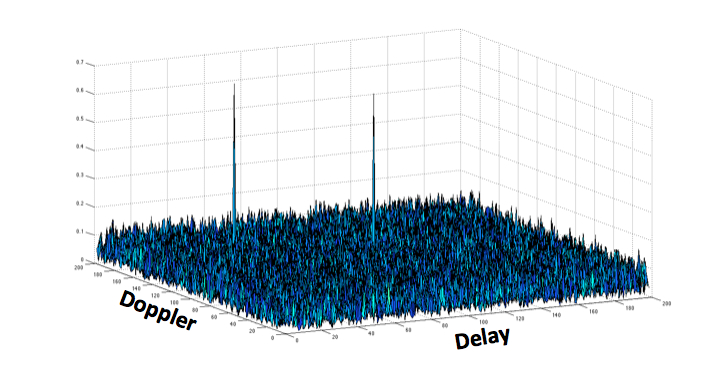
Figure 3: Profile of $\mathcal{A}(\varphi,H(\varphi))$, for $\varphi$ PR, $N=199,$ and channel parameters $(50,150)$, $(100,100),$ $(150,50),$ with attenuation coefficients $0.7,$ $0.7,$ $0.1,$ respectively. Note the insensibility of the channel parameter $(150,50)$ associated with the small attenuation coefficient.

Remark I-B.2

We have

1. Arithmetic Complexity. The arithmetic complexity of the pseudo-random method is $O(N^{2}\log N),$ using Remark I-B.1.

2. Large Deviation of Attenuation Coefficients. From Identity (I-B.5), we deduce that the pseudo-random method will fail to detect delay-Doppler parameter $\left(\tau_{k},\omega_{k}\right)$ associated with attenuation coefficient $\alpha_{k}$ which is small in magnitude compare to $\mathop{\textstyle\sum}\widetilde{\alpha}_{j}/\sqrt{N}.$ We illustrate this in Figure 3, where the channel parameter $(150,50)$ can not be detected because it is associated with the small attenuation coefficient equal to $0.1.\vskip 6.0pt plus 2.0pt minus 2.0pt$

3. Noise. From (I-B.3) we conclude that, a target is detectable by the pseudo-random method only if the associated attenuation coefficient is of magnitude larger than $\sqrt{2\log\log N}/\sqrt{N\cdot SNR}.$

I-C Arithmetic Complexity Problem

For applications to sensing, that require sufficiently high frequency resolution, we will need to use sequences of large length $N$ (see Remark I-A.2). In this case, the arithmetic complexity $O(N^{2}\log N)$ of the pseudo-random method might be too high. Note that to compute one entry of the ambiguity function already takes $N$ operations.

Problem I-C.1 (Arithmetic Complexity)

Solve Problem I-A.1, with method for extracting the channel parameters (I-A.3), which requires almost linear arithmetic complexity.

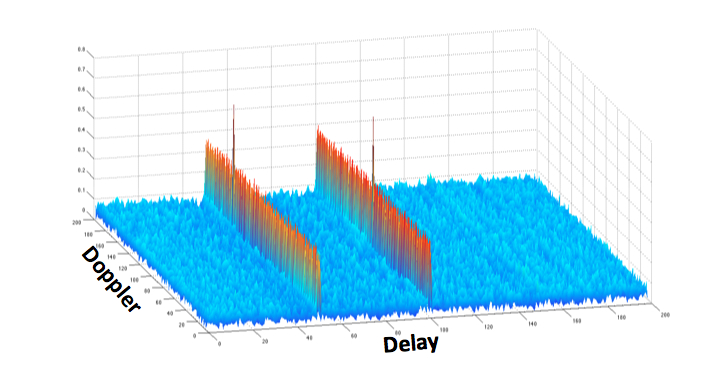
Figure 4: Profile of $\mathcal{A(}f_{L},H(f_{L}))$ for flag $f_{L},$ $L=\{(0,\omega)\},$ $N=199,$ and channel parameters $(50,150)$, $(100,100),$ with attenuation coefficients $0.7,$ $0.7,$ respectively.

In [1] the flag method was introduced in order to deal with the complexity problem. It computes $r$ channel parameters in $O(rN\log N)$ arithmetic operations. For a given line $L$ in the plane $\mathbb{Z}_{N}\times\mathbb{Z}_{N},$ one construct a sequence $f_{L}$—called flag—with ambiguity function $\mathcal{A(}f_{L},H(f_{L}))$ having special profile—see Figure 4 for illustration. It is essentially supported on shifted lines parallel to $L$, that pass through the delay-Doppler shifts (I-A.3), and have peaks there. This suggests a simple algorithm to extract the channel parameters. First compute $\mathcal{A(}f_{L},H(f_{L}))$ on a line $M$ transversal to $L,$ and find the shifted lines on which $\mathcal{A(}f_{L},H(f_{L}))$ is supported. Then compute $\mathcal{A(}f_{L},H(f_{L}))$ on each of the shifted lines and find the peaks. The overall complexity of the flag algorithm is therefore $O(rN\log N)$, using Remark I-B.1.

In these notes we suggest radar detection methods, that, in the multi-target regime, have much better arithmetic complexity.

I-D Inhomogeneous Radar Scene Problem

We would like to estimate the channel parameters (I-A.3) also in the case of large deviation of attenuation coefficients (see Remark I-B.2). This task arises in inhomogeneous radar scene, i.e., in attempt to sense small targets in the vicinity of large objects—see Figure 5 for illustration.

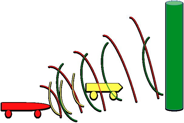
Figure 5: Car radar (red) transmits waveform, and receives echo from car (yellow) and tower (green).

Problem I-D.1 (Inhomogeneous Radar Scene)

Solve Problem I-A.1 in the case of large deviation of attenuation coefficients.

Remark I-D.2

We note that both the pseudo-random and flag methods [1] use pseudo-random sequences. Hence, their applicability for inhomogeneous radar scene is limited (see Figure 3).

I-E Solutions to the Arithmetic Complexity and Inhomogeneous Radar Scene Problems

In these notes we introduce the Incidence and Cross methods, which estimate the channel parameters in complexity of $O(N\log N+r^{3}),$ and $O(N\log N+r^{2})$, respectively. This is a striking improvement over the flag and pseudo-random methods, in the realistic sparsity regime $r\ll N.$ In addition, the incidence and cross methods suggest solutions to the inhomogeneous radar scene problem. Both methods use the special sequences called chirps. This makes them attractive for real world applications, since the commonly used Linear Frequency Modulated (LFM) radar employs chirp sequences.

Remark I-E.1

A more comprehensive treatment of the incidence and cross methods, including further development, statistical analysis, and proofs, will appear elsewhere.

II Chirp Sequences

In this section we introduce chirp sequences, and discuss their correlation properties. In addition, we recall their eigenfunction property for a certain commuting family of Heisenberg operators.

II-A Definition of the Chirp Sequences

We have $N+1$ lines in the discrete delay-Doppler plane $V=\mathbb{Z}_{N}\times\mathbb{Z}_{N}.$ For each $a\in\mathbb{Z}_{N}$ we have the line $L_{a}=\left\{(\tau,a\tau);\tau\in\mathbb{Z}_{N}\right\}$ of finite slope $a,$ and in addition we have the line of infinite slope $L_{\infty}=\left\{(0,\omega);\text{ }\omega\in\mathbb{Z}_{N}\right\}.$ We define the orthonormal basis for $\mathcal{H}$ of chirp sequences associated with $L_{a}$

$$\mathcal{B}_{L_{a}}=\left\{C_{L_{a,b}}\text{; }b\text{ }\in\mathbb{Z}_{N}\right\},$$

where

$$C_{L_{a,b}}[n]=e(2^{-1}an^{2}-bn)/\sqrt{N},n\in\mathbb{Z}_{N}.$$

In addition, we have the orthonormal basis of chirp sequences associated with $L_{\infty}$

$$\mathcal{B}_{L_{\infty}}=\left\{C_{L_{{}_{\infty},b}}\text{ ; }b\text{ }\in\mathbb{Z}_{N}\right\},$$

where

$$C_{L_{{}_{\infty},b}}=\delta_{b},$$

denotes the Dirac delta sequence supported at $b.$ The chirp sequences satisfy—see Figure 6 for illustration—the following properties:

Theorem II-A.1 (Correlations)

We have

1. Auto-correlation. For every $a,b\in\mathbb{Z}_{N}$

   $$\mathcal{A}(C_{L_{a,b}},C_{L_{a,b}})[v]=\left\{\begin{array}[]{c}e(b\tau)\text{ \ if }v=(\tau,a\tau);\\ 0\text{ \ \ \ \ \ if }v\notin L_{a}.\text{ \ }\end{array}\right.$$

   In addition, for every $b\in\mathbb{Z}_{N}$

   $$\mathcal{A}(C_{L_{\infty,b}},C_{L_{\infty,b}})[v]=\left\{\begin{array}[]{c}e(b\omega)\text{ \ if }v=(0,\omega);\\ \text{ \ }0\text{ \ \ \ \ if }v\notin L_{\infty}.\text{ \ }\end{array}\right..$$

2. Cross-correlation. For every two lines $L\neq M\subset V$, and every $C_{L}\in\mathcal{B}_{L},C_{M}\in\mathcal{B}_{M},$

   $$\left|\mathcal{A(}C_{L},C_{M})[v]\right|=1/\sqrt{N},$$

   for every $v\in V.\vskip 3.0pt plus 1.0pt minus 1.0pt$

Figure 6: Plot (real part) of $\mathcal{A}(C_{L_{1,1}},C_{L_{1,1}}),$ for chirp $C_{L_{1,1}}[n]=e[2^{-1}n^{2}-n]$, associated with line $L_{1}=\{(\tau,\tau)\}.$

II-B Chirps as Eigenfunctions of Heisenberg Operators

The Heisenberg operators (I-B.1) satisfy the commutation relations

$$\pi(\tau,\omega)\pi(\tau^{\prime},\omega^{\prime})=e(\omega\tau^{\prime}-\tau\omega^{\prime})\cdot\pi(\tau^{\prime},\omega^{\prime})\pi(\tau,\omega),$$ (II-B.1)

for every $(\tau,\omega),(\tau^{\prime},\omega^{\prime})\in V.$ In particular, for a given line $L\subset V,$ we have the family of commuting operators $\pi(l),$ $l\in L.$ Hence they admit an orthonormal basis for $\mathcal{H}$ of common eigenfunctions. Important property of the chirp sequences is that $\mathcal{B}_{L}$ is such a basis of eigenfunctions. Indeed, it is easy to check that for every $a,b\in\mathbb{Z}_{N}$

$$\pi(\tau,a\tau)C_{L_{a,b}}=e(b\tau)C_{L_{a,b}},\text{ }\tau\in\mathbb{Z}_{N},$$ (II-B.2)

and in addition for every $b\in\mathbb{Z}_{N}$

$$\pi(0,\omega)C_{L_{\infty,b}}=e(b\omega)C_{L_{\infty,b}},\text{ \ }\omega\in\mathbb{Z}_{N}.$$ (II-B.3)

Remark II-B.1

A function $\psi:L\rightarrow\mathbb{C}^{\ast}$, where $L\subset V$ is a line, is called character if $\psi(l+l^{\prime})=\psi(l)\psi(l^{\prime})$, for every $l,l^{\prime}\in L.$ Note that the functions $\psi_{a,b}:L_{a}\rightarrow\mathbb{C}^{\ast},$ $\psi_{a,b}(\tau,a\tau)=$ $e(b\tau),$ and $\psi_{\infty,b}:L_{\infty}\rightarrow\mathbb{C}^{\ast},$ $\psi_{\infty,b}(0,\omega)=$ $e(b\omega),$ are characters, of $L_{a},$ and $L_{\infty},$ respectively. Sometimes, we will write equations (II-B.2), (II-B.3) in one compact form

$$\pi(l)C_{L}=\psi_{L}(l)C_{L},\text{ }l\in L,\text{ }$$

where $C_{L}\in\mathcal{B}_{L\text{ }}$is a chirp, and $\psi_{L}$ is a character.

III Radar Detection using Chirps and the Matching Problem

One of the reasons to use chirps for radar detection, is their advantage in the case of inhomogeneous radar scene. Let us elaborate on this. We define the support of the channel operator $H$ (I-A.1) to be the set $supp(H)=\{\left(\tau_{k},\omega_{k}\right);$ $k=1,...,r\}.\vskip 6.0pt plus 2.0pt minus 2.0pt$

Definition III-.1 ($L$-genericity)

Let $L\subset V$ be a line.

1. We say that a subset $X\subset V$ is generic with respect to $L,$ if for every $u,v\in X$ we have $u-v\notin L.\vskip 6.0pt plus 2.0pt minus 2.0pt$

2. We say that the channel operator $H$ is $L$-generic, if $supp(H)$ is generic with respect to $L$.

Proposition III-.2 (Genericity)

The probability $P,$ that a subset $\left\{v_{1},...,v_{r}\right\}\subset V$ is generic with respect to a randomly chosen line $L\subset V$, satisfies

$$P\geq 1-\frac{r^{2}-r}{2(N+1)}.$$

Remark III-.3

It follows from Proposition III-.2, that in the case $r\ll N^{\frac{1}{2}}$, the channel operator is generic, with high probability, with respect to a randomly chosen line.

Assume that $H$ is $L$-generic. Then by Theorem II-A.1, for a chirp $C_{L}\in\mathcal{B}_{L}$ we have

$$\left|\mathcal{A}(C_{L},H(C_{L}))[v]\right|$$ (III-.1)

$$= \left\{\begin{array}[]{c}\left|\alpha_{k}\right|\text{ \ if }v\in L+(\tau_{k},\omega_{k}),\text{ }k=1,...,r;\\ \text{ \ \ }0\text{ \ \ \ \ \ \ \ \ \ \ \ \ \ otherwise, \ \ \ \ \ \ \ \ \ \ \ \ \ \ \ \ \ }\end{array}\right.$$ (III-.4)

where $L+(\tau_{k},\omega_{k})$ denotes the shifted line $\left\{l+(\tau_{k},\omega_{k});\ l\in L\right\}.$

Remark III-.4

The meaning of Identity (III-.1) is that using a chirp we can sense targets associated with small attenuation coefficients.

Suppose we have an additional line $M\neq L,$ such that $H$ is $M$-generic. In particular—see Figure 7 for illustration—computing $\mathcal{A}(C_{L},H(C_{L}))$ on $M,$ we obtain $r$ peaks at points

$$m_{1},...,m_{r}\in M.$$ (III-.5)

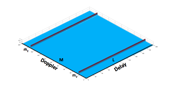
Figure 7: $\left|\mathcal{A(}C_{L},H(C_{L}\mathcal{)})\right|$ with $L=\{(\tau,0)\},$ $r=2,$ and $supp(H)=\{l_{1}+m_{2},$ $l_{2}+m_{1}\}.$

Figure 8: $\left|\mathcal{A(}C_{M},H(C_{M}\mathcal{)})\right|$ with $M=\{(0,\omega)\},$ $r=2,$ and $supp(H)=\{l_{1}+m_{2},$ $l_{2}+m_{1}\}.$

In the same way—see Figure 8 for illustration—computing $\mathcal{A}(C_{M},H(C_{M}))$ on $L,$ we obtain $r$ peaks at points

$$l_{1},...,l_{r}\in L.$$ (III-.6)

Note that every channel parameter (I-A.3) is represented uniquely by a suitable $l_{i}+m_{j}$, for some $i,j$.

Problem III-.5 (Matching)

Find the $r$ points from $l_{i}+m_{j}$, $1\leq i,j\leq r,$ which belong to $supp(H).\vskip 6.0pt plus 2.0pt minus 2.0pt$

In these notes we will propose resolutions to the matching problem, that will be efficient in terms of arithmetic complexity, and work well also if we add to $H$ a reasonable noise sequence $\mathcal{W}$ as in (I-A.2).

IV The Incidence Method

The incidence method is the first resolution for the matching problem that we discuss. The main idea already appears in various places in the literature (see Figure 29 on page 307 of [5]). Our contribution is a low arithmetic complexity implementation of this method, and certain mathematical analysis of its performance.

IV-A The Incidence Method

We use a third chirp $C_{M^{\circ}},$ associated with a third line $M^{\circ}\subset V.$ Assume that $H$ is also $M^{\circ}$-generic. Then we have—see Figure 9 for illustration—that $\mathcal{A}(C_{M^{\circ}},H(C_{M^{\circ}}))$ is supported on $r$ shifted lines, which are parallel to $M^{\circ}$ and pass through the delay-Doppler points that we want to detect. To find these shifted lines we compute—see Figure 9—$\mathcal{A}(C_{M^{\circ}},H(C_{M^{\circ}}))$ on $L,$ and obtain $r$ peaks at points

$$l_{1}^{\circ},...,l_{r}^{\circ}\in L,$$ (IV-A.1)

yielding the $r$ desired shifted lines $M^{\circ}+l_{k}^{\circ},$ $k=1,...,r.$

Under certain additional genericity assumption (see Section IV-B) the solution to Problem III-.5 is exactly the collection of  the points $v_{i,j}=l_{i}+m_{j}$, $1\leq i,j\leq r$, with three shifted lines from $L+m_{j}$’s, $M+l_{i}$’s, $M^{\circ}+l_{k}^{\circ}$’s passing through them—see Figure 10 for illustration. We summarize the computational part of the method in the Incidence Algorithm below.

Incidence Algorithm

Input:

 Chirps $C_{L},C_{M},C_{M^{\circ}}$, associated with randomly chosen lines $L,M,$ and $M^{\circ},$ and corresponding echoes $R_{L},R_{M},R_{M^{\circ}}$, threshold $T>0$, and value of $SNR$.

Output:

    Channel parameters.

1. Compute $\mathcal{A(}C_{M},R_{M}\mathcal{)}$ on $L$, obtain peaks at $l_{1},...,l_{r_{1}}.\vskip 3.0pt plus 1.0pt minus 1.0pt$

2. Compute $\mathcal{A(}C_{L},R_{L}\mathcal{)}$ on $M,$ obtain peaks at $m_{1},...,m_{r_{2}}.\vskip 3.0pt plus 1.0pt minus 1.0pt$

3. Compute $\mathcal{A(}C_{M^{\circ}},R_{M^{\circ}}\mathcal{)}$ on $L,$ obtain peaks at $l_{1}^{\circ},...,l_{r_{3}}^{\circ}.\vskip 3.0pt plus 1.0pt minus 1.0pt$

4. Return the points $v_{i,j}\in V$ that satisfy $v_{i,j}=l_{i}+m_{j}\in M^{\circ}+l_{k}^{\circ},$ $1\leq i\leq r_{1}$, $1\leq j\leq r_{2}$, $1\leq k\leq r_{3}$.

Remark IV-A.1 (Single Transmission)

The incidence method can be modified to work with a single transmission, for sensing targets with slightly larger attenuation coefficients. Indeed, consider the sequence $C_{L,M,M^{\circ}}=\left(C_{L}+C_{M}+C_{M^{\circ}}\right)/\sqrt{3}$ constructed using chirps associated with three different lines. Using Theorem II-A.1, and the normalization $\sum_{k=1}^{r}\left|\alpha_{k}\right|^{2}\leq 1,$ we have

$$\mathcal{A}(C_{K},H(C_{L,M,M^{\circ}}))=\mathcal{A}(C_{K},H(C_{K}))/\sqrt{3}+O(\sqrt{r/N}),$$

where $K=L,M$ or $M^{\circ}.$ In particular, the incidence algorithm above is applicable.

Figure 9: $\left|\mathcal{A(}C_{M^{\circ}},H(C_{M^{\circ}}\mathcal{)})\right|$ with $M^{\circ}=\{(\tau,\tau)\},$ and $supp(H)$ as in Figures 7, and 8.

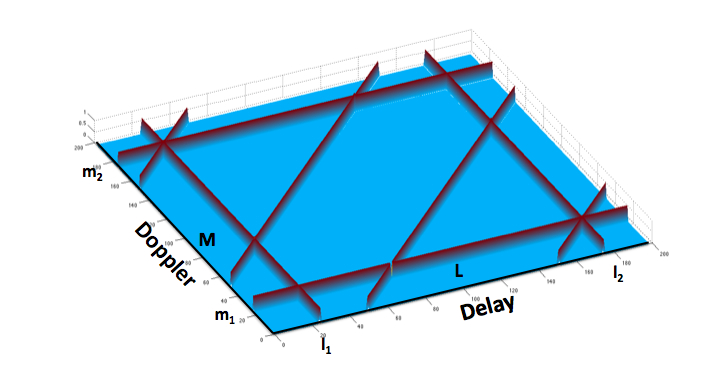
Figure 10: Three chirps are used to obtain correct matching: $l_{1}$ with $m_{2},$ and $l_{2}$ with $m_{1}.$

IV-B Perfectness

For the incidence method to work well we need additional relation, called perfectness, between the channel operator $H$ and the lines $L,M,M^{\circ}.\vskip 6.0pt plus 2.0pt minus 2.0pt$

Definition IV-B.1

We define

1. Let $\mathcal{F}$ be a family of shifted lines in $V.$ A vector $v\in V$ is called incidence point of $\mathcal{F}$, if $v$ is lying on at least two shifted lines from $\mathcal{F}$. The incidence number of incidence point $v$ of $\mathcal{F}$, is the number of shifted lines from $\mathcal{F}$ on which $v$ is lying.

2. A collection of vectors $v_{1},\ldots,v_{r}\in V$ is called perfect with respect to a collection of lines $L_{1},...,L_{d},$ if these are the only incidence points of the family $\mathcal{F=}\{v_{i}+L_{j}\,|\,1\leq i\leq r,$ $1\leq j\leq d\}$ with incidence number $d.\vskip 6.0pt plus 2.0pt minus 2.0pt$

Example IV-B.2

In Figure 10 the vectors $l_{1}+m_{2}$, $l_{2}+m_{1},$ form a perfect collection with respect to the lines $L,M,M^{\circ}.$

Assume now that $r>0$ is given, and that $\#supp(H)=r$. Let us choose at random three lines $L,M,M^{\circ}\subset V$. Assume that $H$ is generic with respect to $L,M,$ and $M^{\circ}$.

Proposition IV-B.3 (Perfectness)

The probability $P$ that $supp(H)$ is perfect with respect to $L,M,M^{\circ}$ satisfies

$$P\geq 1-\frac{r(r^{2}-r)}{N}.$$

IV-C Remarks on Performance

1. Detection. In the noiseless scenario, it follows from Remark III-.3, that in steps 1, 2, 3, of the incidence algorithm above, we have $r_{1}=r_{2}=r_{3}=r$, with probability greater or equal $1-O(r^{2}/N)$. In addition, in this case it follows from Proposition IV-B.3 that the incidence method will return all the channel parameters with probability greater or equal $1-O(r^{3}/N)$.

2. Noise. Combining (I-B.3) and (III-.1), we deduce that in case of genericity and perfectness of $supp(H)$ with respect to the three randomly chosen lines, the incidence algorithm will detect the delay-Doppler shifts (I-A.3) associated with attenuation coefficients of magnitude larger then $(T+1)\sqrt{2\log\log N}/\sqrt{N\cdot SNR}$ with probability going to one, as $N$ goes to infinity.

3. Arithmetic Complexity. Using Remark I-B.1, we can compute all the $l_{i}$’s, $m_{j}$’s, and $l_{k}^{\circ}$’s, in $O(N\log N)$ operations. The verification of which of the $r^{2}$ points $l_{i}+m_{j},$ $1\leq i,j\leq r,$ lie on one of the shifted lines $M^{\circ}+l_{k}^{\circ}$ requires order of $r^{3}$ arithmetic operations. Overall, the arithmetic complexity of the incidence method is $O(N\log N+r^{3}).\vskip 6.0pt plus 2.0pt minus 2.0pt$

4. Real Time. Applicability of incidence method for inhomogeneous radar detection requires the transmission of three chirps. For time-varying channel this might be not useful [5].

V The Cross Method

The cross method is the second resolution for the matching problem that we discuss. We show how to use the values—including the phase and not just the amplitude—of the ambiguity function, to suggest a solution to the matching problem. This method does not require transmission of additional chirp, and has lower arithmetic complexity.

Figure 11: The values $\mu_{j}=\mathcal{A}(C_{L},H(C_{L}))[m_{j}],$ $j=1,2,$ are used for resolving the matching problem.

Figure 12: The values $\lambda_{i}=\mathcal{A}(C_{M},H(C_{M}))[l_{i}],$ $i=1,2,$ are used for resolving the matching problem.

V-A The Cross Method

Consider chirps $C_{L},C_{M},$ associated with the lines $L,M$ and characters $\psi_{L}:L\rightarrow\mathbb{C}^{\ast},$ $\psi_{M}:M\rightarrow\mathbb{C}^{\ast}$, respectively. This means (see Section II-B) that we have the eigenfunction identities $\pi(l)C_{L}=\psi_{L}(l)C_{L}$, and $\pi(m)C_{M}=\psi_{M}(m)C_{M},$ for every $l\in L,$ $m\in M.$ Let us assume that the channel operator $H$ is generic with respect to $L$ and $M$. We have—see Figures 11,12 for illustration—the peak values

$$\left\{\begin{array}[]{c}\mathcal{A}(C_{L},H(C_{L}))[m_{j}],\text{ \ }j=1,...,r;\\ \mathcal{A}(C_{M},H(C_{M}))[l_{i}],\text{ \ }i=1,...,r,\end{array}\right.$$

where $m_{1},...,m_{r}\in M,$ $l_{1},...,l_{r}\in L,$ are the points given by (III-.5), and (III-.6), respectively. To resolve the matching problem, we define hypothesis function $h:L\times M\rightarrow\mathbb{C}$ by

$$h(l,m) = \mathcal{A}(C_{L},H(C_{L}))[m]\cdot\psi_{L}[l]$$

$$-\mathcal{A}(C_{M},H(C_{M}))[l]\cdot e(\Omega[l,m])\cdot\psi_{M}[m],$$

where $\Omega:V\times V\rightarrow\mathbb{Z}_{N}$ is given by $\Omega[(\tau,\omega),(\tau^{\prime},\omega^{\prime})]=\tau\omega^{\prime}-\omega\tau^{\prime}.\vskip 6.0pt plus 2.0pt minus 2.0pt$

Theorem V-A.1 (Matching)

Suppose $l_{i}+m_{j}\in supp(H),$ then $h(l_{i},m_{j})=0.\vskip 6.0pt plus 2.0pt minus 2.0pt$

Remark V-A.2

The conclusion in Theorem V-A.1 is not necessarily true if $H$ is not generic with respect to $L$ or $M.\vskip 6.0pt plus 2.0pt minus 2.0pt$

Remark V-A.3 (Algebraic Genericity)

Under natural (genericity) assumptions on the channel operator, and for random choice of chirps, the ”converse” of Theorem V-A.1 is true with high probability, i.e., if $h(l_{i},m_{j})$ $\approx 0,$ $1\leq i,j\leq r$, then with high probability $l_{i}+m_{j}\in supp(H).$ A more precise formulation and development of this statistical aspect will be published elsewhere.

We summarize the computational part of the method in the Cross Algorithm below.

Cross Algorithm

Input:

 Chirps $C_{L},C_{M}$, associated with randomly chosen lines $L,M$, and randomly chosen characters $\psi_{L},\psi_{M}$; corresponding echoes $R_{L},R_{M};$ thresholds $T_{1},T_{2}>0$, and the value of $SNR$.

Output:

    Channel parameters.

1. Compute $\mathcal{A}(C_{M},R_{M})$ on $L,$ and take the $r_{1}$ peaks located at points $l_{i},$ $1\leq i\leq r_{1}\vskip 3.0pt plus 1.0pt minus 1.0pt$.

2. Compute $\mathcal{A}(C_{L},R_{L})$ on $M,$ and take the $r_{2}$ peaks located at the points $m_{j},1\leq j\leq r_{2}\vskip 3.0pt plus 1.0pt minus 1.0pt$.

3. Return the points $v_{i,j}=l_{i}+m_{j}$, which solve $|h(l_{i},m_{j})|\leq T_{2}\sqrt{2\log\log(N)}/\sqrt{N\cdot SNR}$, where $1\leq i\leq r_{1},1\leq j\leq r_{2}$.

Remark V-A.4 (Single Transmission)

The cross method can be modified to work with a single transmission, for sensing targets with slightly larger attenuation coefficients. Indeed, consider the sequence $C_{L,M}=\left(C_{L}+C_{M}\right)/\sqrt{2}$ constructed using chirps associated with two different lines. Using Theorem II-A.1, and the normalization $\sum_{k=1}^{r}\left|\alpha_{k}\right|^{2}\leq 1,$ we have

$$\mathcal{A}(C_{K},H(C_{L,M}))=\mathcal{A}(C_{K},H(C_{K}))/\sqrt{2}+O(\sqrt{r/N}),$$

where $K=L,M.$ In particular, the cross algorithm above is applicable.

V-B Remarks on Performance

We have

1. Detection. In the noiseless scenario, it follows from Remark III-.3, that in steps 1, 2, of the cross algorithm above, we have $r_{1}=r_{2}=r$, with probability greater or equal $1-O(r^{2}/N)$. In addition, in this case it is not hard to see that the cross algorithm will return all the channel parameters with probability greater or equal $1-O(r^{2}/N)$.

2. Arithmetic Complexity. Using Remark I-B.1, we can compute all the $l_{i}$’s, $m_{j}$’s, (III-.6), (III-.5), in $O(N\log N)$ operations. The computation for which of the $r^{2}$ pairs $l_{i},m_{j},$ $1\leq i,j\leq r,$ the hypothesis function $h(l_{i},m_{j})$ is sufficiently small, requires order of $r^{2}$ arithmetic operations. Overall, the arithmetic complexity of the cross method is $O(N\log N+r^{2}).\vskip 6.0pt plus 2.0pt minus 2.0pt$

3. Real Time. Applicability of cross method for inhomogeneous radar detection requires the transmission of two chirps.

VI Conclusions

In these notes we present the incidence and cross methods for efficient radar detection. These methods, in particular, suggest solutions to two important problems. The first is the inhomogeneous radar scene problem, i.e., sensing small targets in the vicinity of large object. The second problem is the arithmetic complexity problem. Low arithmetic complexity enables higher velocity resolution of moving targets. We summarize these important features in Figure 13, and putting them in comparison with the flag and pseudo-random (PR) methods.

Figure 13: Comparing methods, with respect to arithmetic complexity for $r$ targets, and sensibility of targets in terms of magnitude of attenuation coefficients (noiseless scenario).

Acknowledgements. We are grateful to our collaborators A. Sayeed, and O. Schwartz, for many discussions related to the research reported in these notes. We appreciate the contributions of I. Bilik, U. Mitra, K. Scheim, and E. Weinstein, who shared with us some of their thoughts on radar detection. We thank the students of the course ”applied algebra”, that took place at UW - Madison in Fall 2013, and in particular we acknowledge the Ph.D. students J. Lima, S. Qinyuan, and Z.M. Arslan. Finally, we thank the Max Planck Institute for Mathematics at Bonn, and the Mathematics Department at the Weizman Institute for Science, where part of this document was drafted during July-August 2013.

References

• [1] Fish A., Gurevich S., Hadani R., Sayeed A., and Schwartz O., Delay-Doppler Channel Estimation with Almost Linear Complexity. Accepted for publication in IEEE Transaction on Information Theory (2013).
• [2] Golomb, S.W., and Gong G., Signal design for good correlation. For wireless communication, cryptography, and radar. Cambridge University Press, Cambridge (2005).
• [3] Gurevich S., Hadani R., and Sochen N., The finite harmonic oscillator and its applications to sequences, communication and radar . IEEE Transactions on Information Theory, vol. 54, no. 9, September 2008.
• [4] Howard S. D., Calderbank, R., and Moran W., The finite Heisenberg–Weyl groups in radar and communications. EURASIP J. Appl. Signal Process (2006).
• [5] Levanon N., Stepped-frequency pulse-train radar signal. IEEE Proc. - Radar, Sonar and Navigation, 149 (6), 297-309, 2002.
• [6] Rader C. M., Discrete Fourier transforms when the number of data samples is prime. Proc. IEEE 56, 1107–1108 (1968).
• [7] Tse D., and Viswanath P., Fundamentals of Wireless Communication. Cambridge University Press (2005).
• [8] Verdu S., Multiuser Detection, Cambridge University Press (1998).
• [9] Wang Z., and Gong G., New Sequences Design From Weil Representation With Low Two-Dimensional Correlation in Both Time and Phase Shifts. IEEE Transactions on Information Theory, vol. 57, no. 7, July 2011.