Trapping of Spin-0 fields on tube-like topological defects

Abstract

We have considered the localization of resonant bosonic states described by a scalar field $\Phi$ trapped in tube-like topological defects. The tubes are formed by radial symmetric defects in $(2,1)$ dimensions, constructed with two scalar fields $\phi$ and $\chi$, and embedded in the $(3,1)-$dimensional Minkowski spacetime. The general coupling between the topological defect and the scalar field $\Phi$ is given by the potential $\eta F(\phi,\chi)\Phi^{2}$. After a convenient decomposition of the field $\Phi$, we find that the amplitudes of the radial modes satisfy Schrödinger-like equations whose eigenvalues are the masses of the bosonic resonances. Specifically, we have analyzed two simple couplings: the first one is $F(\phi,\chi)=\chi^{2}$ for a fourth-order potential and, the second one is a sixth-order interaction characterized by $F(\phi,\chi)=(\phi\chi)^{2}$. In both cases the Schrödinger-like equations are numerically solved with appropriated boundary conditions. Several resonance peaks for both models are obtained and the numerical analysis showed that the fourth-order potential generates more resonances than the sixth-order one.

I introduction

Topological defects are full of interesting realizations in physics. As examples one can cite applications in the study of quark confinement phenom , gravitation and cosmology cosm and condensed matter physics condmat . The idea that we live in a multidimensional brane world brane-origins has been applied to the issue of topological defects, with interesting insights to the problem of cosmological constant and hierarchy br1 ; br2 ; br3 ; br4 ; br5 . The inclusion of scalar fields is connected to the concept of dynamically generated thick branes thick1 ; thick2 ; thick3 ; thick4 ; thick5 ; thick6 ; thick7 ; thick8 ; thick9 ; thick10 ; thick_rev with interesting results concerning to their structure, collision properties and localization of fields field-localiz .

In this work we study a class of topological defects embedded in a flat spacetime. Despite the absence of gravity, the defects are in a way similar to $(5,1)$ branes, in the sense of being the result of an embedding of a topological defect in two extra dimensions. Specifically we consider $(2,1)$-dimensional topological defects with two coupled real scalar fields, constructed within a simplified model describing a color dielectric medium. We follow and extend the procedure presented in Refs. bmm1 ; bmm2 for the case of two real scalar fields. We show that the embedding of the radial defect in $(3,1)$ -dimensions form a tube-like topological defect and study its structure. In the present work, we show that the construction with two scalar fields is crucial for studying processes of field localization of spin-0 particles with particular interest for resonance effects.

There are several examples of two-dimensional topological defects with radial symmetry. For instance, vortices are $(2,1)$ dimensional soliton solutions in $U(1)$ gauge theory with complex scalars and the Higgs mechanism vortex . Recently, interesting extensions for non-Abelian fields have been constructed nonabelian . Ring-type objects are a subject of great interest (see, for instance, the review rv ). An important example of solutions of this type in curved spacetime are black rings, which are solutions of general relativity with extra dimensions (see, for instance, er ). Another interesting example of ring solitons in gauge field theory are the anomalous solitons, where the gauge field is constrained after fixing its Chern-Simons number by including fermions into the system rt ; rub . Also in non-Abelian gauge field theory we can have smooth, finite energy loops stabilized by the magnetic energy, forming non-abelian rings. Considering the non-Abelian Yang-Mills-Higgs theory for the group $SU(2)$, ring solitons were obtained in kks which are more general solutions than the magnetic monopoles tp . Other constructions give sphaleron rings kkl . A sphaleron is a static unstable solution of the classical equations of motion; it is a saddle point configuration separating topologically distinct vacua rub2 . Despite their possible instability, the sphaleron rings can perhaps have an importance as mediators of baryon number violating processes km ; rv .

In this work we are interested in the Abelian version of the color dielectric model fried ; wil with two real scalar fields without fermions. The topological defect formed is neither a ring nor a vortex (in the sense that there is no winding number). A first physical motivation is to show that a dielectric model with two coupled real scalar fields can be responsible for an effective breaking of translational invariance, leading to a topological defect capable of trapping scalar particles with simple couplings. In this way, this work can be inserted in a series of previous studies of trapping of spin-0 fields for specific topological defects. In the context of braneworlds there are several examples of such analysis. In $(5,1)$ dimensions (one extra dimension) see, for instance, the works in scalar-localiz . The construction of brane models with one extra dimension can be done starting from the solution in $(1,1)$ dimensions with the help of the first-order formalism thick1 . The first-order formalism is very helpful for achieving explicit analytical solutions for brane models. As far as we know, brane models with two extra dimensions have no similar formalism developed yet, which turns explicit solutions much more difficult to obtain. In this way another motivation for this work can be inserted in the searching for such first-order formalism. Indeed, here we consider a $(3,1)-$dimensional system where the two extra dimensions are described by the usual $(y,z)$ coordinates, but where the application of a first-order formalism was done only in a flat Minkowski spacetime, neglecting gravity effects.

The manuscript is presented in the following way: In Section II we consider $(2,1)$-dimensional radial topological defects embedded in a $(3,1)$-dimensional flat spacetime. In Section III, we study some aspects of localization of scalar fields in this system, and numerically investigate resonance effects in Section IV. Our conclusions are presented in Section V.

II A TUBE IN (3, 1)-DIMENSIONS

We start with an Abelian version of the color dielectric model fried ; wil without fermions. We can express this by the following action

$$S = \int dtdxdydz\biggl{[}\frac{1}{2}\partial_{M}\phi\partial^{M}\phi+\frac{1}{2}\partial_{M}\chi\partial^{M}\chi$$ (2)

$$-\frac{g(\phi,\chi)}{4}F_{MN}F^{MN}-eA_{M}J^{M}\biggr{]},$$

where $g(\phi,\chi)$ is the electric permittivity. We use capital letters $M$, $N$ for all $(3,1)$ dimensions (coordinates $(t,x,y,z)$) and Greek letters $\mu,\nu$ for $(1,1)$ dimensions (coordinates $(t,x)$). We particularize to $\displaystyle J_{M}=\frac{1}{r}(\delta(r),0,0,0)$, with $r=\sqrt{y^{2}+z^{2}}$, representing the charge density. The factor $1/r$ comes from expressing the delta function $\delta(\vec{r})$ in cylindrical coordinates.

The equations of motion for static and radial scalar fields are

$$\nabla^{2}\phi = -\frac{1}{2}g_{\phi}E^{2},$$ (3)

$$\nabla^{2}\chi = -\frac{1}{2}g_{\chi}E^{2},$$ (4)

where in this paper we use the simplified notation $f_{\phi}=\partial f/\partial\phi$, $f_{\phi\chi}=\partial^{2}f/(\partial\phi\partial\chi)$ and similar constructions for other derivatives of a differentiable function $f$. The Maxwell equations, $\partial_{M}(gF^{MN})=eJ^{N}$ lead to the following expression for the electric field

$$E=\frac{e}{rg}\,\,.$$ (5)

We consider a medium with electric permittivity given by (similar relation for one field was found in bmm1 )

$$g(\phi,\chi)=\frac{e^{2}}{2V(\phi,\chi)},$$ (6)

where

$$V(\phi,\chi)=\frac{1}{2}(W_{\phi}^{2}+W_{\chi}^{2})$$ (7)

is a potential that generates a two-field topological defect in $(1,1)$ dimensions and $W(\phi,\chi)$ is the superpotential. This means that we are considering a dielectric model where the electric permittivity is infinity at the vacua of the potential $V(\phi,\chi)$. In $(1,1)$ dimensions the vacua of the potential are located at $\pm\infty$. However, we are constructing a model in $(3,1)$ dimensions with radial symmetry. We will see then that one of the vacua occurs in $r=0$, meaning a divergent dielectric permittivity along the center of the tube. We can also say that the charge density given by $J^{M}$ polarizes the vacuum, leading to a nontrivial topology.

With Eqs. (6), (3) and (4), the equations of motion for the scalar fields are

$$\frac{1}{r}\frac{d}{dr}\biggr{(}r\frac{d\phi}{dr}\biggr{)} = -\frac{e^{2}}{2r^{2}}\frac{g_{\phi}}{g^{2}}$$

$$= \frac{1}{r^{2}}(W_{\phi}W_{\phi\phi}+W_{\chi}W_{\chi\phi})$$

$$\frac{1}{r}\frac{d}{dr}\biggr{(}r\frac{d\chi}{dr}\biggr{)} = -\frac{e^{2}}{2r^{2}}\frac{g_{\chi}}{g^{2}}$$

$$= \frac{1}{r^{2}}(W_{\phi}W_{\phi\chi}+W_{\chi}W_{\chi\chi}).$$

Following a similar procedure established in bmm1 for one-field defects, for a given superpotential $W$ it can be shown that the solutions of the first-order equations,

$$\frac{d\phi}{dr}=\frac{1}{r}W_{\phi}~{}\ ,~{}\ \frac{d\chi}{dr}=\frac{1}{r}W_{\chi},$$ (10)

are also solutions of the second-order equations (II) and (II).

Therefore, the tube in $(3,1)$-dimension is effectively described by the action

$$S_{tube}=\!\int\!\!dtd^{3}x\left(\frac{1}{2}\partial_{M}\phi\partial^{M}\phi+\frac{1}{2}\partial_{M}\chi\partial^{M}\chi-U(\phi,\chi)\right),$$ (11)

with

$$U(\phi,\chi)=\frac{1}{2r^{2}}(W_{\phi}^{2}+W_{\chi}^{2}),$$ (12)

leading to the same equations of motion for the fields $\phi(r)$ and $\chi(r)$ given by Eqs. (II) and (II).

The explicit dependence of $r=\sqrt{y^{2}+z^{2}}$ follows closely and generalizes for two fields the construction of bmm1 ; bmm2 for evading Derrick-Hobarts’ theorem raj1 ; raj2 ; raj3 . The explicit breaking of translational invariance in the action is present in some scenarios of QCD color1a ; color1b ; color2a ; color2b ; deconf , brane intersections br-inta ; br-intb , noncommutative field theory n-coma ; n-comb and condensed matter physics dobr ; bor .

In this work we consider the following superpotential bsr

$$W(\phi,\chi)=\lambda\left(\phi-\frac{1}{3}\phi^{3}-s\phi\chi^{2}\right),$$ (13)

corresponding to the potential

$$U(\phi,\chi)=\frac{\lambda^{2}}{r^{2}}\biggl{(}\frac{1}{2}(1-\phi^{2}-s\chi^{2})^{2}+2s^{2}\phi^{2}\chi^{2}\biggr{)},$$ (14)

which generates kink-like and lump-like solutions given, respectively, by (more general solutions for this model where found in Ref. igg )

$$\phi(r) = \frac{\left(\frac{r}{r_{0}}\right)^{4\lambda s}-1}{\left(\frac{r}{r_{0}}\right)^{4\lambda s}+1}\,\mathrm{\ },$$

$$\chi(r) = \pm 2\sqrt{\frac{1}{s}-2}\,\frac{\left(\frac{r}{r_{0}}\right)^{2\lambda s}}{\left(\frac{r}{r_{0}}\right)^{4\lambda s}+1}.$$

With the condition $0<s<1/2$, the solutions provide a radial profile with $r_{0}$ identified with the radius of the tube’s cross section. The profiles for the $\phi,\chi$ fields are shown in Fig. 1. There it is shown that for increasing $\lambda$ the defect becomes narrower. Also it is verified that for small values of $s$, the effects of the field $\chi$ are more predominant than those of $\phi$ and we have a wider defect. On the other hand, larger values of $s$ show that the $\chi$ field is responsible for the process of generating a thicker tube. In particular, the limit $s=1/2$ recovers the one-field $\phi$ limit and a result from the literature (the solution for $p=1$ in the notation of ref. bmm1 ) is recovered.

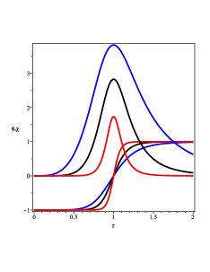
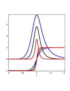
Figure 1: The functions $\phi(r)$ (kink-like) and $\chi(r)$ (lump-like). We fix $r_{0}=1$. We have a) $\lambda=30$ (left) and b) $\lambda=50$ (right). In all figures $s=0.06$ (blue), $s=0.1$ (black), $s=0.2$ (red).

In $(1,1)$ dimensions the potential given by $(W_{\phi}^{2}+W_{\chi}^{2})~{}/2$ has minima at $(\pm 1,0)$ and $(0,\pm\sqrt{1/s})$ with $s>0$; static solutions from the equations of motion connect the minima $(\pm 1,0)$ and form Bloch walls bsr , which are defects with an internal structure given by the $\chi$ field. The limit $s\rightarrow 0.5$ turns the two-field problem into a one-field model with solution known as Ising wall. In the present work the presence of the field $\chi$ also contributes to generate an internal structure to the tube formed. Later in this work we will see that this is crucial for localizing scalar fields with both fourth- and sixth-order potentials.

The energy density of the $2$-dimensional radial defect is

$$T_{00} = 8\left(\frac{\lambda s}{r_{0}}\right)^{2}\frac{\left(\frac{r}{r_{0}}\right)^{4\lambda s-2}}{\left(\frac{r}{r_{0}}\right)^{4\lambda s}+1}$$

$$~{}\times\left\{4\left(\frac{r}{r_{0}}\right)^{4\lambda s}+\left(\frac{1}{s}-2\right)\left[\left(\frac{r}{r_{0}}\right)^{4\lambda s}-1\right]^{2}\right\}$$

Here we consider $T_{00}$ finite in $r=0$, which restricts the parameters to satisfy $\lambda s\geq\frac{1}{2}$ when $\lambda>1$.

For fixed $\lambda>1$ and $\frac{1}{2\lambda}\leqslant s<\frac{1}{2}$, $T_{00}(r)$ changes from a lump centered in $r=0$ $\left(s=\frac{1}{2\lambda}\right)$ to a peak centered around $r_{0}$ $\left(s=\frac{1}{2}\right)$. For larger values of $\lambda$ and lower values of $s$, the contribution of the $\chi$ field is higher and the defect appears as a thick tube structure whose center is localized between the origin and $r_{0}$. On the other hand, for larger values of $\lambda$ and larger values of $s$, the defect looks like as a thin tube centered around $r_{0}$, and the field $\phi$ has the stronger contribution to the energy density.

The total energy in the $yz-$plane is given by $E=8\pi\lambda/3$, which can be identified with the mass of the $(2,1)$ radial topological defect, that is, the total mass (per unit length of the x-direction) of the tube.

III Spin-0 localization

We consider a scalar field $\Phi$ in a region where exists a radial defect constructed with the scalar fields $\phi,\chi$. In the present analysis we neglect the backreaction on the defect by considering that the interaction between the scalar fields is sufficiently weak in comparison to the self-interaction that generates the defect. In the following, we designate $\Phi$ as the weak field, and $\phi,\chi$ the strong ones. We write the action describing the system as

$$S_{1}=\int dtdxdydz\left(\frac{1}{2}\partial_{M}\Phi\partial^{M}\Phi-\frac{\eta}{2}F\left(\phi,\chi\right)\Phi^{2}\right),$$ (17)

The  equation of motion of the scalar field is

$$\partial_{\mu}\partial^{\mu}\Phi-\nabla_{T}^{2}\Phi+\eta F\left(\phi,\chi\right)\Phi=0$$

where

$$\partial_{\mu}\partial^{\mu}=\square=\frac{\partial^{2}}{\partial t^{2}}-\frac{\partial^{2}}{\partial x^{2}}~{}\ ,~{}\ \ \nabla_{T}^{2}=\frac{\partial^{2}}{\partial y^{2}}+\frac{\partial^{2}}{\partial z^{2}}$$

We consider a coupling $F\left(\phi,\chi\right)=F\left(r\right)$ and require $\mathcal{\eta}F(r)\rightarrow 0$ for $0\sim r\ll r_{0}$ and for $r\gg r_{0}$. It is possible to decompose the field $\Phi(t,x,y,z)$ as

$$\Phi(t,x,y,z)=\sum_{\ell,n}\varphi_{\ell n}(t,x)\rho_{\ell n}\left(r\right)e^{i\ell\theta},$$ (18)

where $\ell=0,1,2,...$ is related to the angular momentum eigenvalue. The set $\left\{e^{i\ell\theta}\right\}$ is orthogonal in $\theta\in[0,2\pi]$.  The field $\varphi_{\ell n}(t,x)$ satisfies the two-dimensional Klein-Gordon equation

$$\left(\square+m_{\ell n}^{2}\right)\varphi_{\ell n}=0$$ (19)

and the amplitude $\rho_{n\ell}(r)$ satisfies the radial Schrödinger-like equation

$$-\rho_{n\ell}^{\prime\prime}-\frac{1}{r}\rho_{n\ell}^{\prime}+V\left(r\right)\rho_{n\ell}(r)=m_{\ell n}^{2}\rho_{n\ell}(r),$$ (20)

for fixed $\ell$, where the Schrödinger potential is given by

$$V=\frac{\ell^{2}}{r^{2}}+\mathcal{\eta}F.$$ (21)

By requiring that Eq. (20) defines a self-adjoint differential operator in $r\in$ $[0,+\infty)$, the Sturm-Liouville theory  establishes the orthonormality condition for the components $\rho_{n\ell}(r)$,

$$\int_{0}^{\infty}drr\rho_{n\ell}(r)\rho_{m\ell}(r)=\delta_{mn}.$$ (22)

The action given by Eq. (17) can be integrated in the $(y,z)$ dimensions, leading to

$$S_{1}=\int dtdx\sum_{\ell n}\left(\frac{1}{2}\partial_{\mu}\varphi_{\ell n}\partial^{\mu}\varphi_{\ell n}-\frac{1}{2}m_{\ell n}^{2}\varphi_{\ell n}\right).$$ (23)

This shows that the field $\varphi_{\ell n}$ is a massive two-dimensional Klein-Gordon field with mass $m_{\ell n}$.

IV Numerical Results

In this work we consider two simple couplings: i) $F_{1}(\phi,\chi)=\chi^{2}$ which results in a fourth-order potential $\chi^{2}\Phi^{2}$, and ii) $F_{2}(\phi,\chi)=\left(\phi\chi\right)^{2}$  resulting in a sixth-order potential $\left(\phi\chi\right)^{2}\Phi^{2}$. From Eq. (21), the corresponding Schrödinger potentials are

$$V_{1} = \frac{\ell^{2}}{r^{2}}+4\mathcal{\eta}\left(\frac{1}{s}-2\right)\frac{\left(\frac{r}{r_{0}}\right)^{4\lambda s}}{\left[\left(\frac{r}{r_{0}}\right)^{4\lambda s}+1\right]^{2}}$$ (24)

$$V_{2} = \frac{\ell^{2}}{r^{2}}+4\mathcal{\eta}\left(\frac{1}{s}-2\right)\frac{\left(\frac{r}{r_{0}}\right)^{4\lambda s}\left[\left(\frac{r}{r_{0}}\right)^{4\lambda s}-1\right]^{2}}{\left[\left(\frac{r}{r_{0}}\right)^{4\lambda s}+1\right]^{4}}$$ (25)

In order to investigate numerically the massive states, firstly we consider the region near the origin ($r\ll r_{0}$). For $\lambda s\geq 1/2$, the coupling functions $F_{1}$ and $F_{2}$ go to zero as $r^{4\lambda s}$ then potentials are dominated by the contributions of the angular momentum proportional to $1/r^{2}$,

$$V(r)\approx\frac{\ell^{2}}{r^{2}},$$ (26)

and the nonsingular solutions in $r=0$ are

$$\rho_{n\ell}^{\left(0\right)}(r)=J_{\ell}(m_{n}r).~{},\ \ \ell\geq 0$$ (27)

Hence, for each value of $\ell$, Eq. (27) is used as an input for the Runge-Kutta-Fehlberg method that produces a fifth order accurate solution.

We now define the probability for finding scalar modes with mass $m_{\ell n}$ and angular moment $\ell$ inside the tube of radius $r_{0}$ as

$$P_{\ell n}=\frac{\int\limits_{r_{\text{min}}}^{r_{0}}dr~{}r\left[\rho_{\ell n}\left(r\right)\right]^{2}}{\int\limits_{r_{\text{min}}}^{r_{\text{max}}}dr~{}r\left[\rho_{\ell n}\left(r\right)\right]^{2}}.$$ (28)

Here $r_{min}\ll r_{0}$ is used as the initial condition and $r_{max}$ is the characteristic box length used for the normalization procedure, being a value where the Schrödinger potentials are close to zero and where the massive modes oscillate as plane waves.

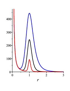
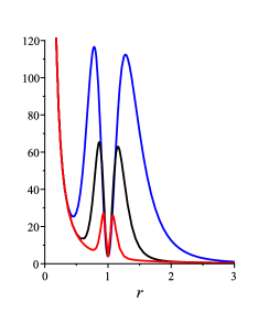
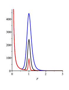
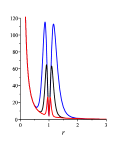
Figure 2: Schrödinger-like potentials $V_{1}$ (left) and $V_{2}$ (right) for $\ell=2$. We fix $r_{0}=1$, and $\eta=30$. We have a) $\lambda=30$ (upper figures) and b) $\lambda=50$ (lower figures). In all figures $s=0.06$ (blue), $s=0.1$ (black), $s=0.2$ (red).

From the energy density considerations of Sec. II, larger values of $\lambda$ favor the existence of a Schrödinger potential with structure similar a tube barrier in $r=r_{0}$.  The Fig. 2 depicts the Schrödinger-like potentials $V_{1}(r)$ and $V_{2}(r)$ for $\ell=2$, $\lambda=30$, $50$, and fixed $\eta=30$ and $r_{0}=1$. The potentials in general diverge in $r\rightarrow 0$, assume a form of a barrier around $r=r_{0}$ (with a local maximum at $r=r_{0}$ for $V_{1}$ and a local minimum for $V_{2}$) and asymptote to zero as $r\rightarrow\infty$, indicating the possible presence of resonances. The increasing of $\eta$ turns the barrier of the potential higher, whereas the increasing of $\lambda$ turns it thinner. We noted that $\ell$ influences on the behavior of the potential for $r<r_{0}$ but has no sensible influence on the barrier. We also observed that the increasing of $r_{0}$ turns wider the potential barrier.

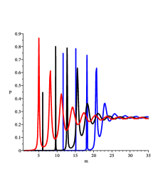
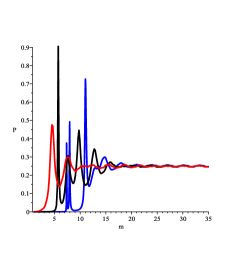
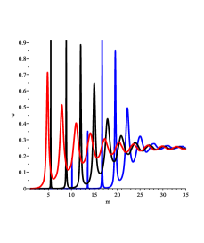
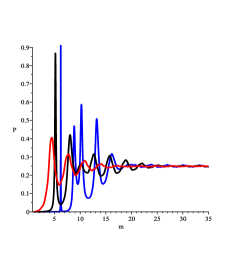
Figure 3: $P_{\ell n}$ as a function of $m$ for couplings $F_{1}=\chi^{2}$ (left) and $F_{2}=(\phi\chi)^{2}$ (right). We fix $\ell=2$, $\eta=30$ and $r_{0}=1$. We have a) $\lambda=30$ (upper figures) and b) $\lambda=50$ (lower figures). In all figures $s=0.06$ (blue), $s=0.1$ (black), $s=0.2$ (red).

We remember that the field $\chi$ is responsible for the internal structure of the defect, present for smaller values of the parameter $s$. This is closely connected to the increasing of the height of the barrier in the Schrodinger potentials, suggesting that lower values of $s$ are more effective for trapping scalar particles. Figs. 3a-b show some results of $P_{\ell n}$ as a function of $m$  for couplings $F_{1}=\chi^{2}$ (left) and $F_{2}=(\phi\chi)^{2}$ (right). The plots are for $\ell=2$, $r_{0}=1$, $\eta=30$ and for various values of $s$ and $\lambda$. We used $r_{min}=10^{-8}$, $r_{max}=4$ and step in $r$ equal to $\Delta r=0.002$. The plots show several peaks of resonances, followed by a plateau for larger masses where $P_{\ell n}=r_{0}/r_{max}$. The thinner is a peak, the larger is the lifetime of the corresponding resonance. Comparing 3a (for $\lambda=30$) with 3b (for $\lambda=50$), we note that, for $\lambda\gg 1$ larger values of $\lambda$ corresponds to slightly less massive resonances, with lower lifetimes. This can be related to the thinner barrier of the Schrodinger potential for larger values of $\lambda$. Also from Figs. 3a-b, we note that lower values of $s$ corresponds to thinner peaks of resonance, agreeing with what expected from analysis of the energy density and Schrodinger potential. The effect of the field $\phi$ in a direct coupling with $\Phi$ is to reduce the effectiveness of the trapping mechanism. This is evident comparing left and right sides from Figs. 3a-b. We note that the resonances with coupling $F_{1}=\chi^{2}$ are better defined, in larger number and with larger masses in comparison with those present when the coupling $F_{2}=(\phi\chi)^{2}$. We also verified that the peak positions do not depend on the choice of $r_{max}$.

V Remarks and conclusions

The present manuscript was firstly motivated by searching a first order formalism in a braneworld scenario with two extra dimensions. We present it in a $(3,1)-$ dimensional system where the $(y,z)-$ coordinates describe extra dimensions, in absence of gravitational effects. The second purpose was to analyze the localization of scalar particles living in a (1+1)-dimensional world (described by $(t,x)-$ coordinates) interacting with a topological defect living in the extra dimensions. In order to show explicitly such implementation, we have considered an Abelian version of the color dielectric model described by two coupled real scalar fields which have generated a tube-like topological defect capable of trapping scalar particles.

Specifically, we have studied the localization of (1+1)-dimensional scalar fields in a generalized tube-like topological defect whose cross-section is a radial defect constructed with two scalar fields. The analysis was performed by considering a general coupling between the defect and the scalar field, and carefully constructed to provide quantum mechanical description of the amplitudes related to the scalar field modes. For the couplings $F(\phi,\chi)=\left(\phi\chi\right)^{2}$   and $F(\phi,\chi)=\chi^{2}$, the numerical analysis of the Hamiltonian spectra showed that the field $\chi$, related to the presence of an internal structure on the defect, is also the main responsible for the mechanism of trapping scalar particles around the tube. Further we must point out that a first-order formalism for two extra dimensions was applied for a problem with axial symmetry in $(3,1)$ dimensions, with interesting analytical simplifications which turned the analysis much easier than a full numerical solution. The present analysis can be considered as a startup in the construction of a first-order formalism for branesworlds with two extra dimensions. In this direction, the study of weak gravity field is currently being considered and results will be reported elsewhere.

References

- (1) J. Greensite, Prog. Part. Nucl. Phys. 51 (2003) 1; T. Suzuki, Nucl. Phys. Proc. Suppl. 30 (1993) 176; M. N. Chernodub,M. I. Polikarpov, in Confinement, Duality, and Nonperturbative Aspects of QCD, p. 387; M. N. Chernodub, V. I. Zakharov, Phys. Rev. Lett. 98 (2007) 082002; M. N. Chernodub, K. Ishiguro, A. Nakamura, T. Sekido, T. Suzuki, V.I. Zakharov, PoSLAT2007, 174 (2007); M.N. Chernodub, Atsushi Nakamura, V.I. Zakharov, Phys.Rev.D78, 074021 (2008).
- (2) A. Anabalon, S. Willison, J. Zanelli, Phys.Rev.D77, 044019 (2008); P. Mukherjee, J. Urrestilla, M. Kunz, A. R. Liddle, N. Bevis, M. Hindmarsh, Phys.Rev.D83, 043003 (2011); M. Sakellariadou, Lect.NotesPhys.738, 359 (2008); P.P. Avelino, C.J.A.P. Martins, C. Santos, E.P.S. Shellard, Phys.Rev.Lett. 89, 271301 (2002); Erratum-ibid. 89, 289903 (2002); P.P. Avelino, L. Sousa, Phys.Rev.D83, 043530 (2011).
- (3) J.C.Y. Teo and C.L. Kane, Phys. Rev. B 82, 115120 (2010); M.A. Silaev and G.E. Volovik, J. Low Temp. Phys, 161, 460 (2010); T. Fukui and T. Fujiwara, Z2 index theorem for Majorana zero modes in a class D topological superconductor, arXiv:1009.2582; T.Sh. Misirpashaev and G.E. Volovik, Physica, B 210, 338 (1995); G.E. Volovik, Pis’ma ZhETF 93, 69 (2011).
- (4) V.A. Rubakov and M.E. Shaposhnikov, Phys. Lett. B 125, 136 (1983); V.A. Rubakov and M.E. Shaposhnikov, Phys. Lett. B 125, 139 (1983); E.J. Squires, Phys. Lett. B 167, 286 (1986); M. Visser, Phys. Lett. B 159, 22 (1985); K. Akama, Lect. Notes Phys. 176, 267 (1982); I. Antoniadis, Phys. Lett. B 246, 377 (1990).
- (5) K. Akama, Lect. Notes Phys. 176, 267 (1982).
- (6) V. A. Rubakov and M. E. Shaposhnikov, Phys. Lett. B 125, 136 (1983).
- (7) V. A. Rubakov and M. E. Shaposhnikov, Phys. Lett. B 125, 139 (1983).
- (8) K. Akama, Gauge Theory and Gravitation, Proceedings, edited by K. Kikkawa, N. Nakanishi, and H. Nariai, Springer-Verlag, Nara, Japan (1983).
- (9) M. Visser, Phys. Lett. B 159, 22 (1985).
- (10) O. DeWolfe, D. Z. Freedman, S. S. Gubser and A. Karch, Phys. Rev. D 62, 046008 (2000).
- (11) M. Gremm, Phys. Lett. B 478, 434 (2000).
- (12) M. Gremm, Phys. Rev. D 62, 044017 (2000).
- (13) A. Kehagias and K. Tamvakis, Mod. Phys. Lett. A 17, 1767 (2002).
- (14) C. Csaki, J. Erlich, T. Hollowood and Y. Shirman, Nucl. Phys. B 581, 309 (2000).
- (15) A. Campos, Phys. Rev. Lett. 88, 141602 (2002).
- (16) R. Guerrero, A. Melfo and N. Pantoja, Phys. Rev. D 65, 125010 (2002).
- (17) D. Bazeia, C. Furtado and A. R. Gomes, J. Cosmol. Astropart. Phys. 0402 (2004) 002.
- (18) D. Bazeia and A. R. Gomes, J. High Energy Phys. 05 (2004) 012.
- (19) D. Bazeia, F. A. Brito and A. R. Gomes, J. High Energy Phys. 0411 (2004) 070.
- (20) V. Dzhunushaliev, V. Folomeev and M. Mina- mitsuji, Rep. Prog. Phys. 73, 066901 (2010).
- (21) Y. X. Liu, J. Yang, Z. H. Zhao, Chun-E Fu and Y. S. Duan, Phys. Rev. D 80, 065019 (2009); Y. X. Liu, H. T. Li, Z. H. Zhao, J. X. Li and J. R. Ren, JHEP 0910, 091 (2009); I. Oda, Phys. Lett. B 496, 113 (2000); C.A.S. Almeida, R. Casana, M.M. Ferreira and A.R. Gomes, Phys. Rev. D 79, 125022 (2009).
- (22) D. Bazeia, J. Menezes, and R. Menezes, Phys. Rev. Lett. 91, 241601 (2003).
- (23) D. Bazeia, J. Menezes, R. Menezes, Mod. Phys. Lett. B19, 801 (2005).
- (24) H. B. Nielsen and P. Olesen, Nucl. Phys. B 61, 45 (1973).
- (25) M. Shifman and A. Yung, Rev. Mod. Phys. 79, 1139 (2007). M. Eto, T. Fujimori, S. B. Gudnason, Y. Jiang, K. Konishi, M. Nitta and K. Ohashi, JHEP 1011 (2010) 042. R. Auzzi, S. Bolognesi, J. Evslin, K. Konishi and A. Yung, Nucl. Phys. B673, 187-216 (2003). M. Eto, T. Fujimori, Y. Isozumi, M. Nitta, K. Ohashi, K. Ohta and N. Sakai, Phys. Rev. D 73, 085008 (2006). J. Evslin, Kenichi Konishi, Muneto Nitta, Keisuke Ohashi, W. Vinci, Non-Abelian Vortices with an Aharonov-Bohm Effect, ArXiv 1310.1224 [hep-th].
- (26) R. Emparan and H.S. Reall, Class. Quant. Grav., 23, R169, 2006; ibid, Living Rev.Rel. 11:6,2008.
- (27) V.A. Rubakov and A.N. Tavkhelidze, Phys. Lett. B 165, 109 (1985).
- (28) V. A. Rubakov, Prog. Theor. Phys. 75, 366 (1986).
- (29) B. Kleihaus, J. Kunz, and Y. Shnir. Phys. Rev. D 68, 101701 (2003); Phys. Rev., D 70, 065010 (2004).
- (30) Gerard t́ Hooft, Nucl. Phys. B 79, 276 (1974); A. M. Polyakov. JETP Lett. 20, 194 (1974).
- (31) B. Kleihaus, J. Kunz, M. Leissner, Phys. Lett. B 663, 438 (2008).
- (32) V. A. Rubakov, Classical Theory of Gauge Fields, Princeton Univ. Press, Princeton, 2002.
- (33) F. R. Klinkhamer and N. S. Manton, Phys. Rev. D 30, 2212 (1984).
- (34) E. Radu and M. S. Volkov, Phys. Rept. 468, 101 (2008).
- (35) R. Friedberg and T. D. Lee, Phys. Rev. D15, 1694 (1977); 16, 1096 (1977); 18, 2623 (1978).
- (36) L. Wilets, Nontopological Solitons (World Scientific, Singapore, 1989).
- (37) B. Bajc and G. Gabadadze, Phys. Lett. B 474 (2000) 282. Heng Guo, A. Herrera-Aguilar, Yu-Xiao Liu, D. Malagon-Morejon, R. R. Mora-Luna, Phys.Rev. D87 (2013) 095011. Heng Guo, Yu-Xiao Liu, Zhen-Hua Zhao, Feng-Wei Chen, Phys.Rev. D85 (2012) 124033.
- (38) R. Hobart, Proc. Phys. Soc. Lond.82, 201(1963).
- (39) G. H. Derrick J. Math. Phys. 5, 1252 (1964).
- (40) R. Rajaraman, Solitons and Instantons, North-Holland, Amsterdan, 1982.
- (41) M. Alford, J.A. Bowers, and K. Rajagopal, Phys. Rev. D 63, 074016 (2001).
- (42) M. G. Alford, K. Rajagopal, T. Schaefer, A. Schmitt, Rev.Mod.Phys.80, 1455 (2008).
- (43) R.Casalbuoni, R. Gatto, M. Mannarelli and G. Nardulli, Phys. Lett. B 511, 218 (2001);
- (44) R.Casalbuoni, R. Gatto, M. Mannarelli and G. Nardulli, Phys.Rev. D66 (2002) 014006.
- (45) F. Sannino, N. Marchal, W. Schäfer, Phys.Rev. D66 (2002) 016007.
- (46) N. Arkani-Hamed, S. Dimopoulos, G. Dvali, and N. Kaloper, Phys. Rev. Lett. 84, 586 (2000);
- (47) N. Kaloper, Phys. Lett. B 474, 269 (2000).
- (48) P.-M. Ho and Y.-T. Yeh, Phys. Rev. Lett. 85, 5523 (2000).
- (49) O. Bertolami and L. Guisado, J. High Energy Phys. 12, 013 (2003).
- (50) R.L. Dobrushin, Theor. Prob. Appl.17, 582 (1972).
- (51) C. Borgs, Commun. Math. Phys.96, 251 (1984)
- (52) D. Bazeia, M.J. dos Santos and R.F. Ribeiro, Phys. Lett. A208, 84 (1995).
- (53) A. Alonso Izquierdo, M.A. Gonzalez Leon, J. Mateos Guilarte, Phys.Rev. D65 (2002) 085012.