FTPI-MINN-13/34, UMN-TH-3305/13

September 17/2013

Degeneracy between Abelian and Non-Abelian Strings

Sergei Monin,^a M. Shifman,^b

^aDepartment of Physics, University of Minnesota, Minneapolis, MN 55455, USA

^bWilliam I. Fine Theoretical Physics Institute, University of Minnesota, Minneapolis, MN 55455, USA

Abstract

In a model that supports both Abelian (Abrikosov-Nielsen-Olesen) and non-Abelian strings we analyze the parameter space to find examples in which these strings not only coexist but are degenerate in tension. We prove that both solutions are locally stable, i.e there are no negative modes in the string background. The tension degeneracy is achieved at the classical level and is expected to be lifted by quantum corrections. The set up of the model, analogous to that of Witten’s superconducting cosmic strings, had been extended to include non-Abelian strings previously [2].

1 Introduction

This paper can be viewed as a logical continuation of [2, 3, 4]. Topologically stable non-Abelian strings which were discovered [5] in 2003 significantly extended the class of the (local) stringy solitons which essentially had been limited previously to the Abrikosov-Nielsen-Olesen (ANO) strings [6]. A natural question arises as to whether the ANO (i.e. Abelian) and non-Abelian strings can coexist in one and the same model, both being locally stable, and if yes, whether their tensions can be degenerate. The exact answer to the second question can be given only in supersymmetric models provided that both strings are BPS-saturated [7], with one and the same central charge.

Deferring this task for the future here we will explore a simple non-supersymmetric model [2] which extends Witten’s superconducting cosmic strings [8] to find whether or not (classically) degenerate Abelian and non-Abelian strings are simultaneously supported in this model for at least some values of parameters. We will analyze the parameter space to find examples of degenerate strings which are locally stable, i.e there are no negative modes in the string background.

We mainly follow the recent publication [4] to (numerically) construct profile functions with zero and non-zero values of the triplet field $\chi$, i.e. Abelian vs. non-Abelian. To justify the quasiclassical approximation we assume weak coupling in the bulk. First, to normalize our calculation, we determine the profile functions corresponding to the Abrikosov-Nielsen-Olesen string and find its tension. Next, we find the string solution with non-zero $\chi$. We show that with the appropriate choice of the parameters the two strings are degenerate in tension at the classical level (within the accuracy of our numerical calculations). We also investigate stability of the strings.

2 Formulation of the problem

The model in which we will analyze string-like solitons is described by the Lagrangian

$${\cal L}={\cal L}_{0}+{\cal L}_{\chi}$$ (1)

where

$${\cal L}_{0} = -\frac{1}{4e^{2}}F_{\mu\nu}^{2}+\left|{\mathcal{D}}^{\mu}\phi\right|^{2}-V(\phi)\,,$$

$${\mathcal{D}}_{\mu}\phi = (\partial_{\mu}-iA_{\mu})\phi\,,$$

$$V = \lambda\left(|\phi|^{2}-v^{2}\right)^{2}\,,$$ (2)

and

$${\cal L}_{\chi} = \partial_{\mu}\chi^{i}\,\partial^{\mu}\chi^{i}-U(\chi,\phi)\,,$$ (3)

$$U = \gamma\left[\left(-\mu^{2}+|\phi|^{2}\right)\chi^{i}\chi^{i}+\beta\left(\chi^{i}\chi^{i}\right)^{2}\right],$$ (4)

with $i=1,2,3$. We will assume that $\lambda,\beta,\gamma>0$ and $v^{2}>\mu^{2}$. This model has the U(1) gauge symmetry, while the $\chi$ sector is O(3) symmetric. The $\chi$ fields are real.

The potential $V(\phi)$ ensures the Higgsing of the $U(1)$ photon. The complex scalar field $\phi$ develops a nonvanishing vacuum expectation value (VEV),

$$|\phi|=v\,.$$

As a result of the Higgs mechanism the phase of the comlex field is eaten up and becomes photon’s longitudinal component. The photon mass is

$$m^{2}_{A}=2e^{2}v^{2}\,.$$ (5)

The physical Higgs excitation obviously has the mass

$$m^{2}_{\phi}=4\lambda v^{2}\,.$$ (6)

As can be seen from (4), the triplet field $\chi^{i}$ does not condense in the vacuum. Its mass is

$$m^{2}_{\chi}=\gamma\left(v^{2}-\mu^{2}\right).$$ (7)

For what follows it is convenient to introduce three auxiliary dimensionless parameters:

$$a=\frac{m^{2}_{A}}{m^{2}_{\phi}}\equiv\frac{e^{2}}{2\lambda}\,,\quad b=\frac{m^{2}_{\chi}}{m^{2}_{\phi}}\equiv\frac{\gamma}{4\lambda}\,\frac{c-1}{c}\,,\quad c=\frac{v^{2}}{\mu^{2}}\,.$$ (8)

As was discussed in [4], a constraint on the parameters of the Lagrangian exists from the requirement of vacuum stability, namely,

$$\beta\geq\beta_{*}\equiv\frac{b}{c(c-1)}\,.$$ (9)

Other than that the parameters $e$, $\lambda$, $\beta$, $\mu$, and $v$ can be chosen at will. We will assume them to be chosen in such a way that the bulk model is weakly coupled and, hence, the quasiclassical approximation is applicable.

$\beta$	$\displaystyle\frac{\tilde{\lambda}}{\gamma}$
$a$	$\displaystyle\frac{m_{A}^{2}}{m_{\phi}^{2}}$
$b$	$\displaystyle\frac{m_{\chi}^{2}}{m_{\phi}^{2}}$
$\displaystyle\frac{v^{2}}{\mu^{2}}\equiv c$	$\displaystyle\left(1-\frac{4\lambda}{\gamma}\frac{m_{\chi}^{2}}{m_{\phi}^{2}}\right)^{-1}$

Table 1: Parameters in (2), (4) in terms of the particle masses and the coefficients in front of the quartic terms $\phi^{4}$, $\chi^{4}$, and $\phi^{2}\chi^{2}$ ($\lambda$, $\tilde{\lambda}$, and $\gamma$, respectively).

Table 1 shows how the parameters in (2), (4) and $a,b,c$ are related to the masses of the particles involved and the coefficients in front of the quartic terms $\phi^{4}$, $\chi^{4}$ and $\phi^{2}\chi^{2}$. One can view the latter as “physical” parameters of the problem at hand.

3 Key observation

Since the Lagrangian (1) – (4) does not contain terms linear in $\chi$, classical equations of motion always have a solution with $\chi\equiv 0$. If we set $\chi=0$ from the beginning, our model reduces to the standard scalar QED, which supports the standard ANO string. Needless to say that the latter is topologically stable.

Thus, our task is, in addition to the ANO string, to find a solution with $\chi\neq 0$ in the string core. Then we must check that this solution is (classically) stable under small perturbations with respect to desintegration into the ANO string plus $\chi$ quanta.

4 Anzätze and classical equations

The basic steps of the appropriate construction were discussed in [4, 2, 9]. Here we will only outline its main points. Let us assume that the string lies along the $z$ axis, and introduce a dimensionless radius in the perpendicular $\{x,y\}$ plane,

$$\rho=m_{\phi}\,\sqrt{x^{2}+y^{2}}\,.$$ (10)

If we look for the topologically stable strings, we must make the $\phi$ field wind around the string axis. For simplicity we will assume the minimal (unit) winding. The appropriate ansätze are

$$A_{0}=0\,,\quad A_{i}=-\varepsilon_{ij}\frac{x_{j}}{r^{2}}\left(\rule{0.0pt}{11.38109pt}1-f(r)\right)\,,\quad\phi=v\varphi(\rho)e^{i\alpha}\,,$$ (11)

where $\alpha$ is the polar angle in the perpendicular plane. The boundary conditions are obvious,

$$f(\infty)=0\,,\qquad f(0)=1\,;\qquad\,\varphi(\infty)=1\,,\quad\varphi(0)=0\,.$$ (12)

From Eq. (4) it is clear that the vanishing value of the $\phi$ field in the core of the string may or may not generate a nonvanishing value of the $\chi^{i}$ field. This is a dynamical issue. The $\chi=0$ solution always exists and is stable, while the $\chi\neq 0$ solution may not exist or, if exist, may be classically unstable (i.e. the maximum of theenergy functional rather than its minimum). If the $\chi\neq 0$ solution exists its natural normalization is

$$(\chi^{i}\chi^{i})_{\rm core}\approx\frac{\mu^{2}}{2\beta}\,.$$ (13)

The existence of a stable solution with $\chi\neq 0$ in the core implies that the O(3) symmetry is broken on the string. The appropriate ansatz for $\chi$ is

$$\chi^{i}=\frac{\mu}{\sqrt{2\beta}}\,\chi(\rho)\left(\begin{array}[]{c}0\\ 0\\ 1\end{array}\right)\,,$$ (14)

with the boundary conditions

$$\chi(\infty)=0\,,\quad\chi(0)\approx 1\,.$$ (15)

Since the Lagrangian is O(3) invariant any nontrivial solution (14) will introdice two rotational moduli.

Minimizing the energy functional we derive the system of equations for the profile functions

$$\left(\frac{f^{\prime}}{\rho}\right)^{\prime} = a\frac{\varphi^{2}\,f}{\rho}\,,$$

$$\left(\rule{0.0pt}{11.38109pt}\phi^{\prime}\rho\right)^{\prime} = \frac{f^{2}\,\varphi}{\rho}+\frac{\rho\varphi\left(\varphi^{2}-1\right)}{2}+\frac{\rho\,\varphi\,\chi^{2}}{2\beta}\frac{b}{c-1}\,,$$

$$\left(\rule{0.0pt}{11.38109pt}\chi^{\prime}\rho\right)^{\prime} = \frac{b}{c-1}\rho\chi\left(c\varphi^{2}+\chi^{2}-1\right)\,,$$ (16)

where the primes denote differentiation with respect to $\rho$.

Since our purpose is illustrative – we try to establish the very possibility of coexistence of the Abelian and non-Abelian strings – we will limit ourselves to a particularly interesting choice of one of the parameters,

$$a=1\,,\,\,\,\mbox{ i.e.}\,\,\,m_{\phi}=m_{A}\,.$$ (17)

In the absence of the $\chi$ field this choice would corresponds to critical or Bogomol’nyi-Prasad-Sommerfield (BPS) [7] vortex(srting). The tension of such a string is

$$T_{0}=2\pi v^{2}\,.$$ (18)

In the numerical solution of the equations of motion we set $a=1\,$. The value of $T_{0}$ quoted in (18) is used as a reference point.

5 The $\chi=0$ solution

First we consider $\chi=0$ and $\varphi=\varphi_{0}\equiv\varphi_{\rm ANO}$. One can directly check that this is indeed a solution of the set of of equations (16). As in [4], we follow Witten [8] to investigate the stability of the solution with regards to small $chi$ fluctuations. To this end we write down a (linearized) equation for the $\chi$ modes around the ANO solution. The mode equation takes the form

$$-\psi^{\prime\prime}+\left(b\,\frac{c\varphi^{2}_{0}-1}{c-1}-\frac{1}{4\rho^{2}}\right)\psi=\epsilon\psi\,,\qquad\psi(\rho)\equiv\chi\,\sqrt{\rho}\,.$$ (19)

Foe two representative values of parameters the numerical solution yields

$$\epsilon=\left\{\begin{array}[]{l}0.041\,\,\,\mbox{at}\,\,\,b=0.0987\,,\,\,c=1.17\,,\\[8.53581pt] 0.234\,\,\,\mbox{at}\,\,\,b=1.871\,,\,\,c=2\,.\end{array}\right.$$ (20)

The positivity of $\epsilon$ implies the stability of the $\chi=0$ solution. The tension of the string was found to be

$$\frac{T_{0}}{2\pi v^{2}}=1-O(10^{-7})\,.$$ (21)

The second number on the right-hand side of Eq. (21) represents the accuracy of our numerical computations.

6 The $\chi\neq 0$ solution

Now we will demonstrate that although the above ANO solution is locally stable, the model at hand supports a solution with non-Abelian moduli, i.e. with $\chi\neq 0$.

In the case of $\chi\neq 0$ one can find the asymptotic behavior of the profile functions at $\rho\rightarrow\infty$ by linearizing these equations in this limit,

$$f\sim\sqrt{\rho}\,e^{-\rho}\,,\quad\left(1-\varphi\right)\sim\frac{1}{\sqrt{\rho}}\,e^{-\rho}\,,\quad\chi\sim\frac{1}{\sqrt{\rho}}\,e^{-\sqrt{b}\rho}\,.$$ (22)

Then we integrated Eqs. (16) numerically, keeping $a=1$ and varying parameters $\{b,c,\beta\}$. The plots of the profile functions are shown in Fig. 1. One can note a rather low value of the $\chi$ field in the core. In order for the $\chi$ field not to be smeared by quantum fluctuations we must additionally impose a constraint on the parameters

$$\tilde{\lambda}\ll\frac{\chi^{2}(0)}{2(c-1)}\,.$$ (23)

Fortunately, this is always possible since the value of $\tilde{\lambda}$ is in our hands. The origin of Eq. (23) is as follows. The value of the field $\chi$ in the core of the string should be much larger than the mass, otherwise quasiclassical treatment is not applicable (the condensate of the field should contain many quanta). The mass of the $\chi$ field is given in Eq. (7). The normalization of the field given in Eq. (13) should be modified, taking into account the results of our numerical calculation for $\chi(0)$. Thus, the above ratio is expressed as follows

$$\frac{\chi^{2}_{\rm core}}{m^{2}_{\chi}}=\frac{\mu^{2}}{2\beta}\,\chi^{2}(0)\,\frac{1}{\gamma(v^{2}-\mu^{2})}\gg 1\,,$$ (24)

which reduces to Eq. (23).

Similarly to the consideration in Sec. 5, we determine the lowest eigenvalue of the equation

$$-\psi^{\prime\prime}+\left[\frac{b}{c-1}\left(c\varphi^{2}_{1}-1+3\chi_{1}^{2}\right)-\frac{1}{4\rho^{2}}\right]\psi=\epsilon\psi\,,$$ (25)

where $\;\varphi_{1}$,  and $\;\chi_{1}$  are the solutions presented in Fig. 1. This is necessary to check the stability of $\chi\neq 0$ solution with regards to local variations of $\chi$. The results of numerical calculations yield

$$\epsilon=\left\{\begin{array}[]{l}0.042\,\,\,\mbox{at}\,\,\,b=0.0987\,,\,\,c=1.17\,,\\[8.53581pt] 0.235\,\,\,\mbox{at}\,\,\,b=1.871\,,\,\,c=2\,.\end{array}\right.$$ (26)

We determined the tension of the non-Abelian string,

$$\frac{T_{0}}{2\pi v^{2}}=1-O(10^{-7})\,$$ (27)

which must be compared with Eq. (21). We observe the degeneracy of the two strings (with $\chi=0$ and $\chi\neq 0$).

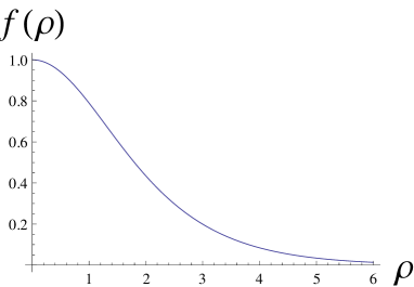
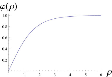
Figure 1: $b=0.0987$, $c=1.17$, $\beta=1.1\beta_{*}$

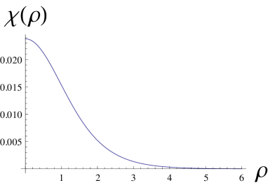
Figure 2: $b=1.871$, $c=2$, $\beta=1.1\beta_{*}$

7 Conclusions

In the model [2] we found numerical solutions for the profile functions and calculated the tensions of two distinct (but degenerate) strings. This proves the possibility of coexistence of the ANO and non-Abelian degenerate strings in one and the same model simultaneously. The classical degeneracy is not protected against quantum corrections. The obvious next step is to supersymmetrize the model to see whether or not one can have the two strings BPS-saturated. Then the degeneracy will be preserved in higher orders. Another interesting project is to slightly change the parameters of the model to make the two strings slightly non-degenerate, with the aim of calculating the decay rate of the heavier string into the lighter one.

References

- [1]
- [2] M. Shifman, Phys. Rev. D 87, 025025 (2013) [arXiv:1212.4823 [hep-th]].
- [3] M. Shifman and A. Yung, Phys. Rev. Lett. 110, 201602 (2013) [arXiv:1303.7010 [hep-th]].
- [4] S. Monin, M. Shifman and A. Yung, Phys. Rev. D 88, 025011 (2013) [arXiv:1305.7292 [hep-th]].
- [5] A. Hanany and D. Tong, JHEP 0307, 037 (2003) [hep-th/0306150]; R. Auzzi, S. Bolognesi, J. Evslin, K. Konishi and A. Yung, Nucl. Phys. B 673, 187 (2003) [hep-th/0307287]; M. Shifman, A. Yung, Phys. Rev. D70, 045004 (2004). [hep-th/0403149]; A. Hanany and D. Tong, JHEP 0404, 066 (2004) [hep-th/0403158].
- [6] A. Abrikosov, Sov. Phys. JETP 32 1442 (1957); H. Nielsen and P. Olesen, Nucl. Phys. B61 45 (1973).
- [7] E. B. Bogomol’nyi, Sov. J. Nucl. Phys. 24, 449 (1976), reprinted in Solitons and Particles, eds. C. Rebbi and G. Soliani (World Scientific, Singapore, 1984) p. 389. M. K. Prasad and C. M. Sommerfield, Phys. Rev. Lett. 35, 760 (1975), reprinted in Solitons and Particles, Eds. C. Rebbi and G. Soliani (World Scientific, Singapore, 1984) p. 530.
- [8] E. Witten, Nucl. Phys. B 249, 557 (1985).
- [9] M. Shifman, Advanced Topics in Quantum Field Theory, (Cambridge University Press, 2012).
- [10]