Abstract

When random walks on a square lattice are biased horizontally to move solely to the right, the probability distribution of their algebraic area can be exactly obtained [1]. We explicitly map this biased classical random system on a non hermitian Hofstadter-like quantum model where a charged particle on a square lattice coupled to a perpendicular magnetic field hopps only to the right. In the commensurate case when the magnetic flux per unit cell is rational, an exact solution of the quantum model is obtained. Periodicity on the lattice allows to relate traces of the $N^{\rm th}$ power of the Hamiltonian to probability distribution generating functions of biased walks of length $N$.

PACS numbers: 05.40.Fb, 05.40.Jc, 05.30.Jp

1 Introduction

It is well-known that the probability distribution for the algebraic area enclosed by closed random walks on a two-dimensional square lattice is related to the Hofstadter model [2] of an electron hopping on a square lattice and coupled to a perpendicular magnetic field. The generating function of the algebraic area probability distribution of walks of length $N$ is formally identified with the trace of the $N^{\rm th}$ power of the Hofstadter Hamiltonian. This mapping has been used in [3] to recover asymptotically Levy’s law [4] and its first $1/N^{2}$ correction. Here we consider random walks biased horizontally to move only to the right, a geometry which is intermediate between 2 and 1 dimensions. For such biased walks the probability distribution of their algebraic area has been exactly obtained in [1]. We are going to relate the generating function of the algebraic area probability distribution of biased walks of length $N$ to the trace of the $N^{\rm th}$ power of the Hamiltonian of a non hermitian Hofstadter-like quantum model. This situation is reminiscent of other biased classical systems mapped on non hermitian quantum models, as for example the TASEP models [5] and their corresponding non hermitian quantum spin chains. It would certainly be rewarding to look at possible physical interpretations, if any, of the non hermitian Hofstadter quantum mechanics discussed here, in particular in relation to the quantum Hall effect. Note that in the asymptotic limit $N\to\infty$ one expects to recover the probability distribution of the algebraic area under a 1d random curve, a distribution which can be easily obtained by more direct means [6].

2 Algebraic area probability distribution generating function for biased random walks on a square lattice

The generating function for the algebraic area probability distribution of closed walks of length $N$ -in the case of closed walks $N$ is necesseraly even- is defined as

$$Z_{N}({\bf q})\equiv\sum_{A=-\infty}^{\infty}C_{N}(A)\,{\bf q}^{A}$$ (1)

where $C_{N}(A)$ is the number, among the ${N\choose{N/2}}^{2}$, of closed walks whose algebraic area is $A$. The mapping to the Hofstadter model is obtained by setting ${\bf q}=e^{i\gamma}$ where $\gamma=2\pi{\boldsymbol{\Phi}}/{\boldsymbol{\Phi}}_{0}$ is the flux ${\boldsymbol{\Phi}}$ through the unit cell in unit of the flux quantum ${\boldsymbol{\Phi}}_{0}=hc/e$.

More generally, the algebraic area of an opened random walk with $M_{1}$ steps right, $M_{2}$ steps left, $L_{1}$ steps up and $L_{2}$ steps down can be defined as those of the closed walk obtained by adding to the end point of the opened walk a vertical path linking it to the horizontal axis where it started from and then adding a horizontal path back to its starting point. For such walks the generating function $Z_{M_{1},M_{2},L_{1},L_{2}}({\bf q})$ for their algebraic area probability distribution obeys the recurrence relation [1, 7]

$$Z_{M_{1},M_{2},L_{1},L_{2}}({\bf q}) = Z_{M_{1},M_{2},L_{1}-1,L_{2}}({\bf q})+Z_{M_{1},M_{2},L_{1},L_{2}-1}({\bf q})$$ (2)

$${}+{\bf q}^{L_{2}-L_{1}}Z_{M_{1}-1,M_{2},L_{1},L_{2}}({\bf q})+{\bf q}^{L_{1}-L_{2}}Z_{M_{1},M_{2}-1,L_{1},L_{2}}({\bf q})\;,$$

with the initial condition $Z_{0,0,0,0}({\bf q})=1$.

Let us recall that if $x$ and $y$ are two operators satisfying $xy={\bf q}yx$ the ${\bf q}$-binomial theorem [8]

$$(x+y)^{N}=\sum_{M=0}^{N}{N\choose M}_{\bf q}y^{N-M}x^{M}\;,$$ (3)

involves the ${\bf q}$-binomial coefficient

$${N\choose M}_{\bf q}\equiv\frac{[N]_{\bf q}!}{[M]_{\bf q}![N-M]_{\bf q}!}\;,$$ (4)

and the q-factorial

$$[L]_{\bf q}!=\prod_{i=1}^{L}{1-{\bf q}^{i}\over 1-{\bf q}}=1(1+{\bf q})(1+{\bf q}+{\bf q}^{2})\cdots(1+{\bf q}+\ldots+{\bf q}^{L-1})\;.$$ (5)

Here formally one has a generalized ${\bf q}$-binomial theorem with four addends

$$(x+y+x^{-1}+y^{-1})^{N}=\sum_{\stackrel{{\scriptstyle\scriptstyle M_{1},M_{2},L_{1},L_{2}}}{{M_{1}+M_{2}+L_{1}+L_{2}=N}}}Z_{M_{1},M_{2},L_{1},L_{2}}({\bf q})y^{-L_{1}}y^{L_{2}}x^{M_{1}}x^{-M_{2}}$$ (6)

where the unknown $Z_{M_{1},M_{2},L_{1},L_{2}}({\bf q})$’s obey (2).

An exact solution of (2) for random walks biased on the horizontal axis to move solely to the right, i.e. $M_{2}=0$, has been obtained in [1]

$$Z_{M_{1},0,L_{1},L_{2}}({\bf q})=\sum_{k=0}^{\min(L_{1},L_{2})}\left[{M_{1}+L_{1}+L_{2}\choose k}-{M_{1}+L_{1}+L_{2}\choose k-1}\right]{M_{1}+L_{1}-k\choose M_{1}}_{\frac{1}{{\bf q}}}{M_{1}+L_{2}-k\choose M_{1}}_{{{\bf q}}}$$ (7)

such that a q-binomial theorem for 3 addends holds

$$(x+y+y^{-1})^{N}=\sum_{\stackrel{{\scriptstyle\scriptstyle M_{1},L_{1},L_{2}}}{{M_{1}+L_{1}+L_{2}=N}}}Z_{M_{1},0,L_{1},L_{2}}({\bf q})y^{-L_{1}}y^{L_{2}}x^{M_{1}}\;.$$ (8)

It is indeed not difficult to prove that (7) is the solution of (2) when $M_{2}=0$.

One can go a step further and "close" such biased walks by enforcing them to return after $N$ steps to the horizontal axis they started from, i.e. $L_{1}=L_{2}$. It means that if one sets $M_{1}=M$, and so $L_{1}=L_{2}={N-M\over 2}$, the generating function for their algebraic area -in the sense defined above- is then

$$Z_{M,0,{N-M\over 2},{N-M\over 2}}({\bf q})=\sum_{k=0}^{{N-M\over 2}}\left[{N\choose k}-{N\choose k-1}\right]{{N+M\over 2}-k\choose M}_{\frac{1}{{\bf q}}}{{N+M\over 2}-k\choose M}_{\bf q}\equiv Z_{N,M}({\bf q})\;.$$ (9)

$Z_{N,M}({\bf q})$ is by construction real.

3 Random walks counting and non hermitian Hofstadter-like quantum mechanics

3.1 Random walks counting

The question we would like to address is : what the exact expression of $Z_{N,M}({\bf q})$ in (9) can tell us on a corresponding Hofstadter-like model in quantum mechanics ? Recall that in the Hofstadter case the counting of closed random walks of length $N$ directly follows from (1) by setting ${\bf q}=1$

$$Z_{N}(1)=\sum_{M=0}^{N/2}{N!\over M!^{2}({N-2M\over 2})!^{2}}={N\choose N/2}^{2}=({1\over 2\pi})^{2}\int_{-\pi}^{\pi}\int_{-\pi}^{\pi}(2\cos k_{x}+2\cos k_{y})^{N}dk_{x}dk_{y}$$ (10)

The quantum spectrum in the RHS of (10) corresponds to the tight-binding Hamiltonian

$$H=T_{x}+T_{x}^{-1}+T_{y}+T_{y}^{-1}$$ (11)

where $T_{x}=e^{ip_{x}/\hbar}$ and $T_{y}=e^{ip_{y}/\hbar}$ for a unit lattice step with Bloch eigenstates

$$e^{ik_{x}x}e^{ik_{y}y}$$ (12)

where both $k_{x}$ and $k_{y}$ are in the interval $[-\pi,\pi]$. The eigenenergies are indeed

$$e^{ik_{x}}+e^{-ik_{x}}+e^{ik_{y}}+e^{-ik_{y}}=2\cos k_{x}+2\cos k_{y}$$ (13)

as in the RHS of (10).

Similarly, in (9), $Z_{N,M}(1)$ counts the number of biased random walks of length $N$ with $M$ steps to the right and ${N-M\over 2}$ steps up and down

$$Z_{N,M}(1)={N!\over M!({N-M\over 2})!^{2}}$$ (14)

For a given $N$, the number of all possible such walks is, if $N$ is even,

$$\sum_{M=0,M{\;\rm even}}^{N}Z_{N,M}(1)=\sum_{M=0,M{\;\rm even}}^{N}{N!\over M!({N-M\over 2})!^{2}}$$ (15)

and if $N$ is odd,

$$\sum_{M=1,M{\;\rm odd}}^{N}Z_{N,M}(1)=\sum_{M=1,M{\;\rm odd}}^{N}{N!\over M!({N-M\over 2})!^{2}}$$ (16)

Both countings are equal to ${1\over 2\pi}\int_{-\pi}^{\pi}(\pm 1+2\cos k_{y})^{N}dk_{y}$: more precisely when $N$ is even

$$\sum_{M=0,M{\;\rm even}}^{N}Z_{N,M}(1)={1\over 2\pi}\int_{-\pi}^{\pi}(\pm 1+2\cos k_{y})^{N}dk_{y}\;,$$ (18)

and when $N$ is odd

$$\sum_{M=1,M{\;\rm odd}}^{N}Z_{N,M}(1)=(\pm 1){1\over 2\pi}\int_{-\pi}^{\pi}(\pm 1+2\cos k_{y})^{N}dk_{y}\;.$$ (19)

In the RHS of (18,19) the spectrum

$$\pm 1+2\cos k_{y}$$ (20)

corresponds again to a tight-binding-like Hamiltonian but with only right hoppings on the horizontal axis

$$H=T_{x}+T_{y}+T_{y}^{-1}$$ (21)

Indeed the eigenstates (12) has now for eigenenergies

$$e^{ik_{x}}+e^{ik_{y}}+e^{-ik_{y}}$$ (22)

If one insists on restricting the Hilbert space to a real spectrum then either $k_{x}=0$ or $k_{x}=\pm\pi$ so that one ends up with

$$1+2\cos k_{y}\quad{\rm or}\quad-1+2\cos k_{y}$$ (23)

i.e. (20).

3.2 Non hermitian Hofstadter-like quantum mechanics

It follows that if one now introduces a magnetic field perpendicular to the lattice the mapping at hand should be between the algebraic area probability distribution of random walks biased horizontally to move only to the right and a non hermitian "Hofstadter-like" quantum mechanics with only right hoppings. In the Landau gauge the quantum Hamiltonian is

$$H_{\gamma}=T_{x}+T_{y}+T_{y}^{-1}$$ (24)

where $T_{x}$ and $T_{y}$ act on a state $\Psi_{m,n}$ at the lattice site $\{m,n\}$ as [12]

$$T_{x}\Psi_{m,n}=\Psi_{m+1,n},\quad T_{y}\Psi_{m,n}=e^{i\gamma m}\Psi_{m,n+1}$$ (25)

and obey the commutation relation

$$T_{x}T_{y}=e^{-i\gamma}T_{y}T_{x},$$ (26)

where, as said above, $\gamma=2\pi{\boldsymbol{\Phi}}/{\boldsymbol{\Phi}}_{0}$ is the flux ${\boldsymbol{\Phi}}$ through the unit cell in unit of the flux quantum ${\boldsymbol{\Phi}}_{0}=hc/e$. The Hamiltonian (24) is non hermitian, therefore it has complex non-physical eigenvalues.

Using translational invariance in the $y$ direction one sets $\Psi_{m,n}=e^{ink_{y}}\Phi_{m}$ to get the eigenenergy equation

$$\Phi_{m+1}+2\cos(k_{y}+\gamma m)\Phi_{m}=E\Phi_{m}$$ (27)

which can be iterated, for any $k\geq 0$, to

$$\Phi_{m+k}=\prod_{r=m}^{m+k-1}(E-2\cos(k_{y}+\gamma r))\Phi_{m}.$$ (28)

4 Commensurate case: exact solution

In the commensurate case where the magnetic flux per plaquette is rational

$$\gamma=2\pi\frac{p}{q}$$ (29)

with relatively prime integers $p$ and $q$, the model can be solved exactly. The flux being rational, one has a Harper-like model [9] of period $q$ on the lattice. Using this periodicity, the eigenfunctions in the periodic potential are such that $\Phi_{m+q}=e^{iqk_{x}}\Phi_{m}$. It follows from (28) that

$$\prod_{r=1}^{q}(E-2\cos(k_{y}+2\pi{p\over q}r))=e^{iqk_{x}}$$ (30)

has to be satisfied. The product in the LHS of (30) is independent of the integer $p$ that from now on will be fixed to $1$. (30) can be easily solved with respect to $E$ thanks to the identity [10]

$$\prod_{r=1}^{q}(a^{2}-2ab\cos\left(k_{y}+\frac{2\pi}{q}r\right)+b^{2})=a^{2q}-2(ab)^{q}\cos(qk_{y})+b^{2q},$$ (31)

valid for any $a,b,q$ and $k_{y}$. Using (31) with $ab=1$ and $a^{2}+b^{2}\equiv E$, one rewrites the product in the LHS of (30) as

$$\prod_{r=1}^{q}(E-2\cos(k_{y}+2\pi{p\over q}r))=P_{q}(E)-2\cos(qk_{y})$$ (32)

where $P_{q}$ is a Chebyshev polynomials of the first kind [11] of degree $q$. Some examples of Chebyshev polynomials are shown in Fig. 1 and Fig. 2.

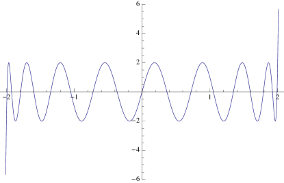
Figure 1: $P_{q=17}(E)$

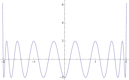
Figure 2: $P_{q=18}(E)$

Setting either $k_{y}=0$ or $\pi/(2q)$ in (32) one obtains

$$P_{q}(E)=\prod_{r=1}^{q}\left(E-2\cos\left(\frac{2\pi r}{q}\right)\right)+2=\prod_{r=1}^{q}\left(E-2\cos\left({\displaystyle\pi\over 2q}+{2\pi r\over q}\right)\right)=2\cos\left(q\arccos\left({E\over 2}\right)\right)$$ (33)

From (30, 32) the eigenenergy equation is

$$P_{q}(E)=e^{iqk_{x}}+2\cos(qk_{y})$$ (34)

and, using (33), one finally gets

$$E_{q}(r)=2\cos\left[\frac{\arccos[e^{iqk_{x}}/2+\cos(qk_{y})]}{q}+\frac{2\pi r}{q}\right],\quad{\rm with}\quad r=1,2,\ldots,q.$$ (35)

or, equivalently,

$$E_{q}(r) = \left({e^{iqk_{x}}/2+\cos(qk_{y})+\sqrt{(e^{iqk_{x}}/2+\cos(qk_{y}))^{2}-1}}\right)^{1/q}$$ (36)

$$+ \left({e^{iqk_{x}}/2+\cos(qk_{y})-\sqrt{(e^{iqk_{x}}/2+\cos(qk_{y}))^{2}-1}}\right)^{1/q},$$

$$\quad{\rm with} \quad r=1,2,\ldots,q.$$

(35) or (36) is the exact spectrum in the commensurate case with arbitrary boundary conditions. For a given such energy, which satisfyes (30), iterating (28) from $m=0$

$$\Phi_{k}=\prod_{r=0}^{k-1}(E-2\cos(k_{y}+2\pi{p\over q}r))\Phi_{0}$$ (37)

gives the exact eigenfunction $\Phi_{k}$ at any lattice site $k=1,2,\ldots$ in terms of a state $\Phi_{0}$ which has to be defined by normalisation considerations.

One has seen that in the absence of a magnetic field $\gamma=0$, or equivalently $q=1$, the spectrum (35) is real when $e^{ik_{x}}=\pm 1$

$$P_{1}(E)=E=e^{ik_{x}}+2\cos k_{y}\to E_{q=1}=\pm 1+2\cos k_{y}\;,$$ (38)

i.e. (20). In the presence of a magnetic field $\gamma=2\pi{p\over q}$ with $q>1$, the spectrum (35) has real eigenvalues only for $e^{iqk_{x}}=\pm 1$. Setting $e^{iqk_{x}}=+1$ corresponds to periodic boundary conditions and $e^{iqk_{x}}=-1$ to anti-periodic boundary conditions on a $q-$cells lattice.

Consider for definiteness periodic boundary conditions. In the region $|1/2+\cos(qk_{y})|<1$ the spectrum consists of $q$ real eigenvalues $|E_{q}|<2$, symmetric around $0$ for even $q$, and it contains $[q/2+1]$ bands. At the points where $|1/2+\cos(qk_{y})|=1$, the spectrum is degenerate with largest eigenvalue $2$ (and by symmetry lowest eigenvalue $-2$ for even $q$). In the region $|1/2+\cos(qk_{y})|>1$ there are only $1$ or $2$ (for odd/even $q$ respectively) real eigenvalues $|E_{q}|\gtrsim 2$, and $q-1$ or $q-2$ complex eigenvalues (see Fig. 3 and Fig. 4).

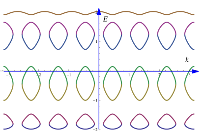
Figure 3: The spectrum $E_{q=7}$ for periodic boundary conditions: on the horizontal axis $k_{y}\in[-\pi,\pi]$, on the vertical axis the energy.

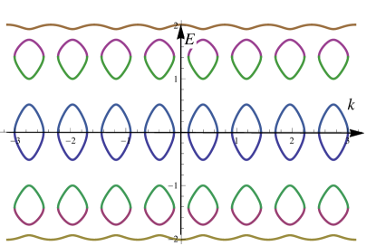
Figure 4: The spectrum $E_{q=8}$ for periodic boundary conditions: on the horizontal axis $k_{y}\in[-\pi,\pi]$, on the vertical axis the energy.

Finally, for large $q$, the density of states with real energy $\rho_{q}(E)$ converges to the 1d tight-binding density of state

$$\rho_{q}(E)\propto\frac{1}{\sqrt{4-E^{2}}}\;.$$ (39)

The edges of the bands are given by the real values of the energy (35) at $k_{y}=0$ and $k_{y}=\pi/q$ (not ordered)

$${\rm for}\;q\;{\rm even:}\;\{2\cos\left({\displaystyle 2\pi\over 3q}+{2\pi r\over q}\right)\;{\rm with}\;r=1,2,\ldots,q,\;\pm 2\cos\left(\frac{{\rm arccos}(3/2)}{q}\right)\},$$

$${\rm for}\;q\;{\rm odd:}\;\{2\cos\left({\displaystyle 2\pi\over 3q}+{2\pi r\over q}\right)\;{\rm with}\;r=1,2,\ldots,q,\;2\cos\left(\frac{{\rm arccos}(3/2)}{q}\right)\}.$$ (43)

A plot of the edge spectrum with periodic boundary conditions for $q=1,2,\ldots,100$ and $p\in[0,q]$ is displayed in Fig. 5.

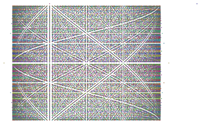
Figure 5: The edge spectrum for periodic boundary conditions: $q=1,2,\ldots,55$, on the horizontal axis the edges and on the vertical axis $p/q\in[0,1]$.

The sum of the lengths of the gaps can be easily computed to be $4/(1+2\cos(2\pi/3q))$ for $q$ even, and $2\cos(\pi/3q)-2/(1+2\cos(\pi/3q))$ for $q$ odd. In the limit $q\to\infty$, it saturates to $4/3$ ($4/3_{+}$ when $q$ even, and $4/3_{-}$ when $q$ odd), whereas the sum of the lengths of the bands saturates to $8/3$ ($8/3_{-}$ for $q$ even, and $8/3_{+}$ for $q$ odd), and the largest and smallest eigenvalues converge to $\pm 2$. A plot of the band spectrum as a function of $1/q$ for $q=1,2,\ldots,100$ is displayed in Fig. 6.

Figure 6: The band spectrum for periodic boundary conditions: $q=1,2,\ldots,100$, on the horizontal axis the bands and on the vertical axis $1/q$.

Note that in the incommensurate case when the flux is irrational the period has to be taken equal to the length $L$ of the lattice. For periodic boundary conditions, one gets from (28) the eigenenergy equation

$$\Phi_{L}=\Phi_{0}\Leftrightarrow\prod_{r=0}^{L-1}(E-2\cos(\gamma r+k_{y}))=1$$ (44)

where the sites $m=0$ and $m=L$ are respectively on the left and right sides of the lattice. A numerical analysis shows that for an arbitrary wave vector $k_{y}$ the spectrum is a mixture of real and complex eigenvalues, see for example Fig. 7.

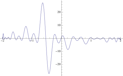
Figure 7: $\prod_{r=0}^{L-1}(E-2\cos(\gamma r+k_{y}))$ for $L=40$, $\gamma=2\pi/\sqrt{2},k_{y}=0$

5 Relation of $TrH(\gamma)^{N}$ to the probability distribution generating function $Z_{N,M}({\bf q})$

In the commensurate case $\gamma=2\pi p/q\to 2\pi/q$ the trace of the Hamiltonian (24) over all eigenvalues -including the complex ones-

$${\rm Tr}H_{\gamma=2\pi/q}^{N}\equiv\int_{-\pi}^{\pi}\frac{dk_{y}}{2\pi}\sum_{r=1}^{q}E_{q}(r)^{N}$$ (45)

should be related to $Z_{N,M}({\bf q})$ in (9) via the mapping ${\bf q}=e^{i\gamma}=e^{i2\pi/q}$. Clearly $q$-cells periodic boundary conditions on the quantum spectrum should imply, for the random walks, summations over $M$ with the same periodicity.

5.1 Periodic boundary conditions $e^{iqk_{x}}=+1$

One can easily check that, when $q$ is even, for any even integer $N$

$${\rm Tr}H_{2\pi/q}^{N}=\sum_{M=0}^{[N/q]}Z_{N,qM}(e^{i2\pi/q})$$ (46)

whereas for any odd integer $N$, trivially,

$${\rm Tr}H_{2\pi/q}^{N}=0$$ (47)

and when $q$ is odd for any even integer $N$

$${\rm Tr}H_{2\pi/q}^{N}=\sum_{M=0}^{[N/(2q)]}Z_{N,2Mq}(e^{i2\pi/q})$$ (48)

and for any odd integer $N$

$${\rm Tr}H_{2\pi/q}^{N}=\sum_{M=0}^{[(N-q)/(2q)]}Z_{N,(1+2M)q}(e^{i2\pi/q})$$ (49)

5.2 Anti-periodic boundary conditions $e^{iqk_{x}}=-1$

Similarly when $q$ is even for any even integer $N$

$${\rm Tr}H_{2\pi/q}^{N}=\sum_{M=0}^{[N/q]}Z_{N,Mq}(e^{i2\pi/q})(-1)^{M}$$ (50)

whereas for any odd integer $N$

$${\rm Tr}H_{2\pi/q}^{N}=0$$ (51)

and when $q$ is odd for any odd even integer $N$

$${\rm Tr}H_{2\pi/q}^{N}=\sum_{M=0}^{[N/(2q)]}Z_{N,2Mq}(e^{i2\pi/q})$$ (52)

and for any odd integer $N$

$${\rm Tr}H_{2\pi/q}^{N}=-\sum_{M=0}^{[(N-q)/(2q)]}Z_{N,(1+2M)q}(e^{i2\pi/q})$$ (53)

Note that when $\gamma=0$, i.e. $q=1$, (48, 49, 52, 53) correctly reproduce (18, 19).

5.3 General boundary conditions $e^{iqk_{x}}\neq\pm 1$

So far, with periodic or antiperiodic boundary conditions, one has satisfied that the spectrum be real when $\gamma=0$ and that, eventhough part of the spectrum is complex when $\gamma\neq 0$, the traces in Sections 5.1 and 5.2 be as well real. One can drop the reality requirement and go a step further by considering general boundary conditions, $e^{iqk_{x}}\neq\pm 1$.

In the case $q$ even, from (46, 50) one infers when $N$ is even

$${\rm Tr}H_{2\pi/q}^{N}=\sum_{M=0}^{[N/q]}Z_{N,Mq}(e^{i2\pi/q})e^{iMqk_{x}}$$ (54)

and when $N$ is odd

$${\rm Tr}H_{2\pi/q}^{N}=0$$ (55)

In the case $q$ odd, from (48, 49, 52, 53) , one arrives when $N$ is even at

$${\rm Tr}H_{2\pi/q}^{N}=\sum_{M=0}^{[N/(2q)]}Z_{N,2Mq}(e^{i2\pi/q})e^{i2Mqk_{x}}$$ (56)

and when $N$ is odd at

$${\rm Tr}H_{2\pi/q}^{N}=\sum_{M=0}^{[(N-q)/(2q)]}Z_{N,(1+2M)q}(e^{i2\pi/q})e^{i(1+2M)qk_{x}}$$ (57)

Note that the RHS of (54, 55, 56, 57) are unchanged if the argument $e^{i2\pi/q}$ in $Z_{N,M}$ is replaced by $e^{i2\pi p/q}$, as it should. Note also that these equations narrow down to the same and unique equation (54) provided that one decides that each time a $Z_{N,M}$ appearing in the sum has entries with different parities, it should be considered as zero: $N$ and $M$ have indeed to have the same parity for the classical random walk to actually exist.

6 Discussion and Conclusion

Motivated by exact results for the probability distribution of the algebraic area of biased random walks, we introduced a quantum mechanical 2d lattice model of charged particles with an anisotropic hopping coupled to a perpendicular uniform magnetic field. An exact solution in the case of a commensurate magnetic flux per unit cell was found with explicit expressions for the eigenvalues and eigenfunctions spectrum. The Hamiltonian is non hermitian due to the anisotropic hopping -the absence of right $\to$ left hopping: it describes a quantum Hall effect setting of enforced left $\to$ right motions for charged particles in a perpendicular magnetic field. As a result, the Hamiltonian has non real eigenvalues which imply a damping of the corresponding states.

We explicitly mapped the biased classical random system on the non hermitian Hofstadter-like quantum model. When the magnetic flux per unit cell is rational, periodicity on the lattice allows to relate the biased length $N$ random walks algebraic area probability generating functions to the traces of the $N^{\rm th}$ power of the non hermitian Hofstadter-like quantum Hamiltonian. The identities (54, 55, 56, 57) are the main results obtained so far: they do encapsulate the mapping between both models. Conversely, it would be interesting to see at a possible geometric interpretation of the RHS of (54, 55, 56, 57) for the biased random walks themselves.

It is interesting to note that one can recover the hermiticity of the Hamiltonian by considering the system with a uniform constant current $J$, so that the Hamiltonian becomes $H-\lambda J$, where $\lambda$ is a Lagrange multiplier, $J=i\sum(\psi^{+}_{n+1}\psi_{n}-\psi^{+}_{n}\psi_{n+1})$ and $H=\sum\psi^{+}_{n+1}\psi_{n}+\ldots$. Then, for the appropriate choice $\lambda=-i/2$, the resulting Hamiltonian becomes hermitian.

Acknowledgements: S.O. would like to thank Stefan Mashkevich for collaboration in the early stages of this work (section 3.1) and Alexios Polychronakos for suggesting to look at general boundary conditions (section 5.3). He would also like to thank Alain Comtet and Christophe Texier for interesting discussions. The help of Etienne Werly has also been precious for some technical details and the plots of the spectra.

References

- [1] S. Mashkevich, S. Ouvry, arXiv:0905.1488, Journal of Statistical Physics, vol 127, issue 1 (2009) 71.
- [2] D.R. Hofstadter, Phys. Rev. B 14 (1976) 2239.
- [3] J. Bellissard, C. Camacho, A. Barelli, F. Claro, J. Phys. A: Math. Gen. 30 (1997) L707.
- [4] P. Lévy, Processus Stochastiques et Mouvements Browniens, Paris, Gauthier-Villars (1965); in Proceedings Second Berkeley Symposium on Mathematical Statistics and Probability, University of California Press (1951) 171.
- [5] see for example the review "The Asymmetric Simple Exclusion Process: An Integrable Model for Non-equilibrium Statistical Mechanics", O. Golinelli and K. Mallick, J. Phys. A: Math. Gen. 39 12679 (2006) and references therein.
- [6] S. Mashkevich, S. Matveenko, S. Ouvry, in preparation.
- [7] C. Béguin, A. Valette, A. Zuk, Journal of Geometry and Physics 21 (1997) 337.
- [8] G.E. Andrews, q-Series: Their Development and Application in Analysis, Number Theory, Combinatorics, Physics, and Computer Algebra. Providence, RI, Amer. Math. Soc. (1986), p. 10.
- [9] P.G. Harper, Proc. Phys. Soc. London A 68 (1955) 874; A 68 (1955) 879.
- [10] A.P. Prudnikov, Yu. A. Brychkov and O.I. Marichev, Integrals and series.Vol. 1 Elementary Functions. Taylor and Francis, London (1986) 755.
- [11] Abramowitz, M. and Stegun, I. A. (Eds.). "Orthogonal Polynomials." Ch. 22 in the Handbook of Mathematical Functions with Formulas, Graphs, and Mathematical Tables, 9th printing. New York: Dover, pp. 771-802, 1972.
- [12] J. Zak, Phys. Rev. A 134, 1602 (1964); Phys. Rev. A 134, 1607 (1964).