Abstract

We consider universal aspects of a holographic Schwinger effect in general backgrounds with an external homogeneous electric field. The argument is based on the potential analysis developed in our previous work. Under some conditions, there always exists a critical electric field, above which the potential barrier vanishes and the system becomes unstable catastrophically. The critical value agrees with the one obtained from the Dirac-Born-Infeld action. For general confining backgrounds, we show that the Schwinger effect does not occur when the electric field is weaker than the confining string tension.

1 Introduction

The Schwinger effect [1] is the pair production of electron and positron in quantum electro dynamics (QED) in the presence of a strong external electric field. This is known as a non-perturbative phenomenon. The production rate is computed under weak-field and weak-coupling conditions [1], and then it is computed only by a weak-field approximation [2] (For the monopole production, see [3]). The pair production is not restricted to QED, but ubiquitous in quantum field theories coupled to an abelian gauge field.

Pairs of virtual particle and anti-particle momentarily created in the vacuum must gain energy more than the total static mass so as to be real particles. This process is described as a tunneling phenomenon with the potential,

$$V(x)=2m-Ex-\frac{\alpha_{\rm s}}{x}\,.$$

Here the first term is the total static mass and then the second is the energy coming from an external electric field $E$ . Finally the third is the Coulomb potential with the fine-structure constant $\alpha_{\rm s}$ . The potential barrier decreases gradually as the electric field becomes stronger, and at last it vanishes at a certain value of the electric field $E=E_{\rm c}$ . This value is called the critical electric field, above which there is no potential barrier and the system becomes unstable catastrophically.

A motive is to understand the critical electric field in the context of string theory [4, 5]. The AdS/CFT correspondence [6, 7, 8] provides a nice laboratory [9]. Semenoff and Zarembo recently proposed a holographic setup to study the Schwinger effect [10]. In this setup, the system is the $SU(N+1)$ $\mathcal{N}=4$ super Yang-Mills theory and the gauge group $SU(N+1)$ is broken to $SU(N)\times U(1)$ by the Higgs mechanism. A probe D3-brane is put at an intermediate position in the bulk AdS space and the mass of the fundamental particles (called “quarks”) is finite. At large $N$ and large ’t Hooft coupling $\lambda\equiv g_{\text{YM}}^{2}N$ , the production rate of quarks with mass $m$ is estimated as [10]

$$\Gamma\sim\exp\left[-\frac{\sqrt{\lambda}}{2}\left(\sqrt{\frac{E_{\text{c}}}{E}}-\sqrt{\frac{E}{E_{\text{c}}}}\,\right)^{2}\right]\,,\qquad E_{\text{c}}=\frac{2\pi m^{2}}{\sqrt{\lambda}}\,.$$ (1.1)

Here $E_{\rm c}$ is the critical electric field and agrees with the result obtained from the Dirac-Born-Infeld (DBI) action. For generalizations of this setup to the case with magnetic fields and the finite temperature case, see [15, 16].

We have revisited the agreement of the critical electric field from the viewpoint of the potential analysis [17]. The probe D3-brane is put at an intermediate position between the horizon and the boundary in the AdS space, as in [10]. Then the quark anti-quark potential is computed from the vacuum expectation value (VEV) of a rectangular Wilson loop on the probe D3-brane by slightly generalizing the methods in [19, 20]. With this quark anti-quark potential, we have shown that the critical electric field agrees with $E_{\rm c}=2\pi m^{2}/\sqrt{\lambda}$ .

This potential analysis is quite a powerful tool because the computation of the VEV of a rectangular Wilson loop is much easier than that of a circular Wilson loop [21, 22]. Hence the potential analysis is applicable to a wide class of systems. A good example is AdS solitons [23] which lead to confinement. For the confining backgrounds, we have shown that there is another critical value of the electric field [24]. When the electric field is smaller than this value, the Schwinger effect does not occur.

It is quite interesting to consider general arguments for the critical electric fields. In this paper we will carry out the potential analysis for general backgrounds and discuss two kinds of the critical electric field. The first is the critical electric field for the catastrophic decay. It universally exists under some conditions for the backgrounds and agrees with the DBI action. This is a generalization of [10] to a certain class of holographic backgrounds. The second is the one, below which the Schwinger effect does not occur, in general confining backgrounds. The sufficient conditions for confining backgrounds are elaborated in [25] (For reviews see [26, 27]). Under the conditions, the critical electric field universally exists.

The organization of this paper is as follows. In section 2, we consider the critical electric field for the catastrophic decay in general backgrounds under some conditions. In section 3, we first introduce the theorem to specify confining backgrounds. For concreteness, two examples are explained. Then we discuss the critical electric field below which the Schwinger effect does not occur. Section 4 is devoted to conclusion and discussion.

2 The catastrophic decay in general backgrounds

We will consider the critical electric field concerning with the catastrophic vacuum decay in general supergravity backgrounds which are constructed basically from D$p$-branes and admit the holographic interpretation.

2.1 Setup

Let us first introduce the setup for our argument. We are concerned with type IIB and IIA supergravity solutions obtained by taking the near-horizon limit of D$p$-brane backgrounds and their generalizations, for which a holographic interpretation is possible.

We assume the diagonal metric for the D$p$-brane world-volume with time $t$ and spatial directions $x^{i}~{}(i=1,\ldots,p)$ . The existence of the radial direction $r~{}(r_{\rm t}\leq r<\infty)$ is also supposed to perform the holographic analysis, where $r_{\rm t}$ is the position of the horizon or the infrared boundary for AdS solitons. For simplicity, we suppose that each component of the metric depends only on $r$ . Thus the metric of the background in ten dimensions is basically given by

$${\rm d}s^{2}=-G_{00}(r){\rm d}t^{2}+\sum_{i=1}^{p}G_{ii}(r)({\rm d}x^{i})^{2}+G_{rr}(r){\rm d}r^{2}+\sum_{m,n=1}^{8-p}G_{mn}(r){\rm d}x^{m}{\rm d}x^{n}\,,$$ (2.1)

where $G_{mn}~{}(m,n=1,\ldots,8-p)$ is the metric of the internal space in $8-p$ dimensions.

The location $r_{\rm t}$ is basically fixed as a zero point of $G_{00}(r)$ in the usual brane setup. For AdS soliton cases $r_{\rm t}$ is given as a zero point of $G_{zz}(r)$ , where $z$ is the compactified direction.

2.2 The potential from the stringy computation

Let us next consider the classical solution of the string world-sheet ending on a probe D-brane located at $r=r_{0}$ . We will work in the Euclidean signature below.

The Nambu-Goto (NG) action is given by

$$S_{\rm NG} =T_{\rm F}\int\!{\rm d}\tau\int\!{\rm d}\sigma\,\mathcal{L}\,,$$ (2.2)

$$\mathcal{L}=\sqrt{\det G_{ab}}\,,\qquad G_{ab}\equiv\frac{\partial x^{\mu}}{\partial\sigma^{a}}\frac{\partial x^{\nu}}{\partial\sigma^{b}}\,g_{\mu\nu}$$ (2.3)

where $\sigma^{a}=(\tau,\sigma)$ are the string world-sheet coordinates.

We are concerned with the potential between a quark and an anti-quark separated in the $x$-direction. For this purpose, it is convenient to take the static gauge,

$$t=\tau\,,\qquad x=\sigma\,,$$ (2.4)

where $x$ is one of the non-compact spatial directions along the D-brane world-volume. The radial direction of the classical solution is supposed to depend only on $\sigma$ ,

$$r=r(\sigma)\,.$$ (2.5)

Under this ansatz, the analysis is drastically simplified.

Using the spacetime metric (2.1) , the Lagrangian is given by

$${\cal L} =\sqrt{f(r)^{2}+g(r)^{2}(\partial_{\sigma}r)^{2}}\,,$$ (2.6)

where we have introduced functions $f(r)$ and $g(r)$ defined as, respectively,

$$f(r)\equiv\sqrt{G_{00}(r)G_{xx}(r)}\,,\qquad g(r)\equiv\sqrt{G_{00}(r)G_{rr}(r)}\,.$$ (2.7)

Here $f(r)$ and $g(r)$ are assumed to be real, smooth and non-negative so that the Lagrangian is well defined. For a holographic interpretation, we suppose a further condition that $f(r)$ is a monotonically increasing function. This condition indicates that the string solution should extend towards the horizon, as we will see later.

Now that the resulting Lagrangian (2.6) depends only on $\sigma$ , the Hamiltonian is a conserved quantity with respect to $\sigma$ . Hence the following relation is obtained,

$${\cal L}-(\partial_{\sigma}r)\frac{\partial{\cal L}}{\partial(\partial_{\sigma}r)}=\frac{f^{2}}{\sqrt{f^{2}+g^{2}(\partial_{\sigma}r)^{2}}}=\mbox{constant}\,.$$ (2.8)

By imposing the boundary condition,

$$r=r_{\rm c}\,,\quad\partial_{\sigma}r=0\quad(\sigma=0)\,,$$ (2.9)

the constant term in (2.8) can be fixed as

$$\frac{f^{2}}{\sqrt{f^{2}+g^{2}(\partial_{\sigma}r)^{2}}}=f(r_{\rm c})$$ (2.10)

and the differential equation is derived,

$$\frac{{\rm d}r}{{\rm d}\sigma}=\pm\frac{f(r)}{g(r)}\frac{\sqrt{f(r)^{2}-f(r_{\rm c})^{2}}}{f(r_{\rm c})}\,.$$ (2.11)

Then the distance $x$ between a quark and an anti-quark is given by

$$x=2\int_{r_{\rm c}}^{r_{0}}\!{\rm d}r\,\frac{g(r)}{f(r)}\frac{f(r_{\rm c})}{\sqrt{f(r)^{2}-f(r_{\rm c})^{2}}}\,,$$ (2.12)

where $r_{0}$ is the position of a probe D-brane. Assume that the above integral is finite. For the geometric relation of the parameters, see Figure 1.

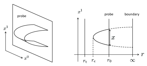
Figure 1: The configuration of the string world-sheet.

In the usual case, the probe D-brane is located near the boundary, namely $r_{0}\to\infty$ . Then the mass of “quark” is infinitely heavy. However, to discuss the pair production in a more realistic setup, the mass should be kept finite and hence the probe D-brane should be put at an intermediate position in the bulk space [10]. Now that $r_{0}$ takes a finite value, the quark mass is given by

$$m=T_{\rm F}\int_{r_{\rm t}}^{r_{0}}\!{\rm d}r\,g(r)\,.$$

This describes the energy of a string stretched between the horizon and the probe D-brane.

On the other hand, for the backgrounds that admit a holographic interpretation, the probe D-brane should be able to be sent to the boundary, in principle. So we assume that the distance $x$ in (2.12) should be finite as a consistency of the background when the $r_{0}\to\infty$ limit is taken. A sufficient condition for this is given by [25]

$$\int_{\tilde{r}}^{\infty}\!{\rm d}r\,\frac{g(r)}{f(r)^{2}}<\infty\,,$$ (2.13)

where $\tilde{r}$ is a certain constant satisfying $\tilde{r}>r_{\rm c}$ . It is easy to show the following inequalities,

$$1<\frac{1}{\sqrt{1-f(r_{\rm c})^{2}/f(r)^{2}}}<\frac{1}{\sqrt{1-f(r_{\rm c})^{2}/f(\tilde{r})^{2}}}\qquad\mbox{for}~{}~{}~{}~{}r>\tilde{r}\,.$$ (2.14)

Then, by multiplying $g(r)/f(r)^{2}$ and integrating from $\tilde{r}$ to $\infty$ , the following integral

$$\int_{\tilde{r}}^{\infty}\!{\rm d}r\,\frac{g(r)}{f(r)^{2}}\frac{1}{\sqrt{1-f(r_{\rm c})^{2}/f(r)^{2}}}$$ (2.15)

is shown to be finite due to the condition (2.13) . With (2.15) , one can see that $x$ is finite when $r_{0}$ is sent to $\infty$ . In other words, the condition (2.13) ensures the finiteness of the distance $x$ for an arbitrary mass, so that the quark and anti-quark potential can definitely be defined. Although it seems unnecessary to take care of heavy mass in studying the Schwinger effect, the pair creation may occur even for heavy particles in principle and we suppose the condition (2.13) for completeness.

According to the conventional AdS/CFT dictionary, the area of the string world-sheet ending on a rectangular Wilson loop leads to the sum of the quark anti-quark potential energy (PE) and the static energy (SE). This is also the case when the probe D-brane is located at an intermediate position $r=r_{0}$ , rather than near the boundary. The resulting potential is given by

$$V_{\rm PE+SE}=T_{\rm F}\int\!{\rm d}\sigma\,\mathcal{L}=2T_{\rm F}\int_{r_{\rm c}}^{r_{0}}\!{\rm d}r\,\frac{g(r)f(r)}{\sqrt{f(r)^{2}-f(r_{\rm c})^{2}}}\,.$$ (2.16)

2.3 The critical electric field from the potential analysis

We shall evaluate the critical electric field by turning on a constant NS-NS two form $B_{tx}=2\pi\alpha^{\prime}E$ . By rewriting (2.16) , the total potential $V_{\rm tot}$ is given by

$$V_{\rm tot} \equiv V_{\rm PE+SE}-Ex$$

$$=T_{\rm F}f(r_{0})(1-\alpha)x+2T_{\rm F}\int_{r_{\rm c}}^{r_{0}}\!{\rm d}r\,\frac{g(r)}{f(r)}\frac{f(r)^{2}-f(r_{\rm c})f(r_{0})}{\sqrt{f(r)^{2}-f(r_{\rm c})^{2}}}\,,$$ (2.17)

where we have introduced a dimensionless quantity $\alpha$,

$$\alpha\equiv\frac{E}{E_{\rm c}}\,,\qquad E_{\rm c}\equiv T_{\rm F}f(r_{0})\,.$$ (2.18)

One can show that the total potential vanishes at $\alpha=1$ ($E=E_{\rm c}$) and exhibits the critical behavior. The proof is straightforward. All we have to do is to show that

$$G(r_{\rm c}(x))\equiv\int_{r_{\rm c}}^{r_{0}}\!{\rm d}r\,\frac{g(r)}{f(r)}\frac{f(r)^{2}-f(r_{\rm c})f(r_{0})}{\sqrt{f(r)^{2}-f(r_{\rm c})^{2}}}$$ (2.19)

is a monotonically decreasing function of $x$ and negative definite. Then the second term in (2.17) does not lift up the potential barrier and whether the potential barrier vanishes or not is relevant only to the first term in (2.17) . For $\alpha<1$ , the potential barrier exists, but it vanishes when $\alpha=1$ . For $\alpha>1$ , there is no barrier any more.

It would be helpful to see the critical behavior from numerical plots of the total potential $V_{\rm tot}(x)$ for fixed geometries. For $\text{AdS}_{5}\times{\rm S}^{5}$ and thermal $\text{AdS}_{5}\times{\rm S}^{5}$ , see Figures 4 and 5 in [17], respectively. For AdS solitons composed of D3-branes and D4-branes, see Figures 2 and 3 in [24], respectively.

Let us then prove that $G(r_{\rm c}(x))$ is a monotonically decreasing function of $x$ and negative definite. The derivative of $G$ with respect to $x$ is written as

$$\frac{{\rm d}G}{{\rm d}x}=\frac{{\rm d}G}{{\rm d}r_{\rm c}}\cdot\frac{{\rm d}r_{\rm c}}{{\rm d}x}\,,$$

and each part is given by, respectively,

$$\frac{{\rm d}G}{{\rm d}r_{\rm c}} =\left(f(r_{\rm c})-f(r_{0})\right)$$

$$\quad\times\lim_{\varepsilon\to 0}\left(-\frac{g(r_{\rm c})}{\sqrt{f(r_{\rm c}+\varepsilon)^{2}-f(r_{\rm c})^{2}}}+\int_{r_{\rm c}+\varepsilon}^{r_{0}}\!{\rm d}r\,\frac{g(r)f(r)f^{\prime}(r_{\rm c})}{(f(r)^{2}-f(r_{\rm c})^{2})^{3/2}}\right)\,,$$ (2.20)

$$\frac{{\rm d}x}{{\rm d}r_{\rm c}} =\lim_{\varepsilon\to 0}\left(-\frac{g(r_{\rm c})}{\sqrt{f(r_{\rm c}+\varepsilon)^{2}-f(r_{\rm c})^{2}}}+\int_{r_{\rm c}+\varepsilon}^{r_{0}}\!{\rm d}r\,\frac{g(r)f(r)f^{\prime}(r_{\rm c})}{(f(r)^{2}-f(r_{\rm c})^{2})^{3/2}}\right)\,.$$ (2.21)

Here a cutoff parameter $\varepsilon$ has been introduced to regularize the integrals. A remarkable point is that the singular parts are canceled out in ${\rm d}G/{\rm d}x$ . Because $f(r)$ is a monotonically increasing function by assumption and $r_{\rm c}\leq r_{0}$ , the following inequality is obtained,

$$\frac{{\rm d}G}{{\rm d}x}=f(r_{\rm c})-f(r_{0})\leq 0\,.$$ (2.22)

Because $G(r_{0})=0$ by definition, where $r_{\rm c}(x=0)=r_{0}$ , $G(r_{\rm c}(x))$ is shown to be a monotonically decreasing function of $x$ and negative definite.

Thus we have shown that $E_{\rm c}$ is the critical value of $E$ . Note that the existence of $E_{\rm c}$ is universal for general backgrounds under the conditions supposed here and the value of $E_{\rm c}$ depends only on a single function $f(r)$ .

2.4 The critical electric field from the DBI action

Let us here argue the critical electric field from the DBI action for a single D$p$-brane. We work in the Lorentzian signature again.

The NG part of the D$p$-brane action is

$$S_{{\rm D}p} =-T_{{\rm D}p}\int\!{\rm d}^{p+1}x\,\sqrt{-\det(g_{\mu\nu}+2\pi\alpha^{\prime}F_{\mu\nu})}\,,$$ (2.23)

where $T_{{\rm D}p}$ is the D$p$-brane tension and the world-volume flux $F_{01}=E$ is turned on. When the probe D-brane is put at $r=r_{0}$ , it can be rewritten as

$$S_{{\rm D}p} =-T_{{\rm D}p}\int\!{\rm d}^{p+1}x\,\prod_{i\neq x}G_{ii}(r_{0})^{1/2}\sqrt{G_{00}(r_{0})G_{xx}(r_{0})-(2\pi\alpha^{\prime})^{2}E^{2}}$$ (2.24)

From this expression, one can read off the critical electric field $E_{\rm c}^{\rm(DBI)}$ and it agrees with the critical value $E_{\rm c}$ obtained by the potential analysis as follows:

$$E_{\rm c}^{\rm(DBI)}=T_{\rm F}\sqrt{G_{00}(r_{0})G_{xx}(r_{0})}=T_{\rm F}f(r_{0})=E_{\rm c}\,.$$ (2.25)

Thus one can see the complete agreement of the critical electric field within a class of the gravitational backgrounds under the current consideration (For concrete examples, see [10, 17, 24]). This implies a universal behavior of the critical electric field.

3 Schwinger effects in general confining backgrounds

We consider here the critical electric field, below which the Schwinger effect does not occur, for general confining backgrounds. We first give a brief review of the sufficient conditions for confining backgrounds argued in [25]. Then we discuss a universal behavior of the critical electric field under the conditions.

3.1 Sufficient conditions for confining backgrounds

Let us first give a review of the theorem in [25]. This would be helpful because our later argument heavily depends on this theorem. It is useful to rewrite (2.16) as

$$V_{\rm PE+SE} = T_{\rm F}f(r_{\rm c})\,x+2T_{\rm F}\int_{r_{\rm c}}^{r_{0}}\!{\rm d}r\,\frac{g(r)}{f(r)}\left[\sqrt{f(r)^{2}-f(r_{\rm c})^{2}}-f(r)\,\right]$$ (3.1)

$$\quad-2T_{\rm F}\int_{r_{\rm t}}^{r_{\rm c}}\!{\rm d}r\,g(r)+2T_{\rm F}\int_{r_{\rm t}}^{r_{0}}\!{\rm d}r\,g(r)\,.$$

The behavior of the potential is essentially determined by the following theorem :
A theorem to specify confining backgrounds

Let us suppose the following five conditions:

1. $f(r)\,,\,g(r)\geq 0$   for   $r_{\rm t}\leq r<\infty$ .

2. $f^{\prime}(r)>0$   for   $r_{\rm t}<r<\infty$ .

3. $\displaystyle\int^{\infty}\!\!{\rm d}r\,\frac{g(r)}{f^{2}(r)}<\infty$  i.e. the integral converges when its upper limit is sent to infinity.

4. $f(r)$ is analytic for $r_{\rm t}<r<\infty$ and is expanded around $r=r_{\rm t}$ like

   $$f(r)=f(r_{\rm t})+a_{k}(r-r_{\rm t})^{k}+\mathcal{O}((r-r_{\rm t})^{k+1})\qquad(k>0~{}~{}\&~{}~{}a_{k}>0)\,,$$ (3.2)

   where $f(r)$ has the minimum at $r=r_{\rm t}$ .

5. $g(r)$ is analytic for $r_{\rm t}<r<\infty$ and is expanded around $r=r_{\rm t}$ like

   $$g(r)=b_{j}(r-r_{\rm t})^{j}+\mathcal{O}((r-r_{\rm t})^{j+1})\qquad(j>-1~{}~{}\&~{}~{}b_{j}>0)\,.$$ (3.3)

Then the potential behavior for sufficiently large $x$ is determined as follows:

1. If $f(r_{\rm t})>0$ and $k=2(j+1)$ , then the linear confinement occurs:

   $$V_{\rm PE+SE}=T_{\rm F}f(r_{\rm t})x-2\kappa+2m+\mathcal{O}((\log x)^{\beta}{\rm e}^{-\gamma x})\,,$$ (3.4)

   where $\kappa$ is given by

   $$\kappa\equiv T_{\rm F}\int_{r_{\rm t}}^{r_{0}}\!{\rm d}r\,\frac{g(r)}{f(r)}\left[f(r)-\sqrt{f(r)^{2}-f(r_{\rm c})^{2}}\,\right]\,.$$ (3.5)

   This is a positive constant and satisfies the inequality $\kappa<m$ . Here $\beta$ and $\gamma$ are positive constants.

2. If $f(r_{\rm t})>0$ and $k>2(j+1)$ , then the linear confinement occurs:

   $$V_{\rm PE+SE}=T_{\rm F}f(r_{\rm t})x-2\kappa+2m-dx^{-\frac{k+2(j+1)}{k-2(j+1)}}+\mathcal{O}(x^{-\delta})\,,$$ (3.6)

   where $\kappa$ is the same as (3.5), $d$ is a positive constant and $\delta$ is given by

   $$\delta\equiv\frac{k+2(j+1)}{k-2(j+1)}+\frac{2}{k-2j}\,.$$

3. If $f(r_{\rm t})=0$ and $k>j+1$ , then the confinement does not occur:

   $$V_{\rm PE+SE}=-A_{\rm s}\,x^{-\frac{j+1}{k-j-1}}+2m+\mathcal{O}(x^{-\delta^{\prime}})\,,$$ (3.7)

   where $A_{\rm s}$ is a constant depending on classical string solutions. Here $\delta^{\prime}$ is given by

   $$\delta^{\prime}\equiv\frac{j+1}{k-j-1}+\frac{2k-j-1}{(2k-j)(k-j-1)}\,.$$

This theorem provides the sufficient conditions to specify general confining backgrounds. Note that the first three conditions have already been imposed. Let us suppose the other conditions below and we consider general confining backgrounds.

Examples

To illustrate the theorem, let us check the conditions for two examples of well-known backgrounds. The first one is AdS solitons, for which the Schwinger effect has already been studied in [24]. The second is confining backgrounds constructed from rotating branes, which have not been discussed in the previous works. For more examples, see [25].

The first example is AdS solitons constructed from D3-branes [23] . The metric in the Lorentzian signature is given by

$${\rm d}s^{2}=\frac{r^{2}}{L^{2}}\left[-({\rm d}x^{0})^{2}+\sum_{i=1}^{2}({\rm d}x^{i})^{2}+\left(1-\frac{r_{\rm t}^{4}}{r^{4}}\right)({\rm d}x^{3})^{2}\right]+\frac{L^{2}}{r^{2}}\left(1-\frac{r_{\rm t}^{4}}{r^{4}}\right)^{-1}{\rm d}r^{2}+L^{2}{\rm d}\Omega_{5}^{2}\,.$$

Here the possible range of $r$ is $r_{\rm t}\leq r<\infty$ . Now suppose that the $x$-direction of the rectangular Wilson loop is taken from either of $x^{1}$ and $x^{2}$ , not $x^{3}$ . From the metric, the following functions are found,

$$G_{00}(r)=G_{xx}(r)=\frac{r^{2}}{L^{2}}\,,\quad G_{rr}(r)=\frac{L^{2}}{r^{2}}\left(1-\frac{r_{\rm t}^{4}}{r^{4}}\right)^{-1}\,.$$

Thus $f(r)$ and $g(r)$ are obtained as

$$f(r)=\frac{r^{2}}{L^{2}}\,,\quad g(r)=\left(1-\frac{r_{\rm t}^{4}}{r^{4}}\right)^{-1/2}\,,$$ (3.8)

and they are manifestly non-negative (The condition 1). Then $f(r)$ is monotonically increasing $f^{\prime}(r)=2r/L^{2}>0$ (The condition 2). It is easy to see the asymptotic behavior,

$$\frac{g(r)}{f(r)^{2}}\sim\frac{L^{4}}{r^{4}}~{}~{}~{}(r\to\infty)\,,$$

hence the condition 3 is satisfied. Note that $f(r)$ has the minimum at $r=r_{\rm t}$ . It is expanded around $r=r_{\rm t}$ like

$$f(r)=\frac{r_{\rm t}^{2}}{L^{2}}+\frac{2r_{\rm t}}{L^{2}}(r-r_{\rm t})+\mathcal{O}((r-r_{\rm t})^{2})\,.$$ (3.9)

Thus $k=1>0$ and $a_{1}=2r_{\rm t}/L^{2}>0$ , and hence the condition 4 is satisfied. Similarly, $g(r)$ is expanded around $r=r_{\rm t}$ as

$$g(r)=\frac{\sqrt{r_{\rm t}}}{2}(r-r_{\rm t})^{-1/2}+\mathcal{O}((r-r_{\rm t})^{1/2})\,.$$ (3.10)

Hence $j=-1/2>-1$ and $b_{-1/2}=\sqrt{r_{\rm t}}/2>0$ , and the condition 5 is also satisfied. Thus the five conditions of the theorem are satisfied.

It is a turn to check the condition to determine whether confinement occurs or not. The minimum of $f(r)$ is positive $f(r_{\rm t})=r_{\rm t}^{2}/L^{2}>0$ . Because $k=1$ and $j=-1/2$ , $k=2(j+1)$ . Thus the AdS soliton backgrounds lead to confinement.

The second example is confining backgrounds constructed from rotating D4-branes [29, 28]. These are a generalization of AdS solitons with an additional parameter. The metric of this background in the Lorentzian signature is given by

$${\rm d}s^{2}= \alpha^{\prime}\frac{2\pi\lambda A}{3u_{0}}u\Delta^{1/2}\left[4u^{2}\eta_{\mu\nu}{\rm d}x^{\mu}{\rm d}x^{\nu}+\frac{4A^{2}}{9u_{0}^{2}}u^{2}\left(1-\frac{u_{0}^{6}}{u^{6}\Delta}\right){\rm d}\theta_{2}^{2}+\frac{4}{u^{2}\left(1-\frac{a^{4}}{u^{4}}-\frac{u_{0}^{6}}{u^{6}}\right)}{\rm d}u^{2}\right.$$

$$\left.\qquad\qquad+{\rm d}\theta^{2}+\frac{\tilde{\Delta}}{\Delta}\sin^{2}\theta\,{\rm d}\varphi^{2}+\frac{1}{\Delta}\cos^{2}\theta\,{\rm d}\Omega_{2}^{2}-\frac{4a^{2}Au_{0}^{2}}{3u^{4}\Delta}\sin^{2}\theta\,{\rm d}\theta_{2}{\rm d}\varphi\right]\,.$$ (3.11)

Here $\Delta\,,\tilde{\Delta}$ and $A$ are defined as, respectively,

$$\Delta\equiv 1-\frac{a^{4}\cos^{2}\theta}{u^{4}}\,,\qquad\tilde{\Delta}\equiv 1-\frac{a^{4}}{u^{4}}\,,\qquad A\equiv\frac{u_{0}^{4}}{u_{H}^{4}-\frac{1}{3}a^{4}}\,.$$ (3.12)

The parameter $a$ represents the angular momentum and $u_{0}$ is the horizon when $a=0$ . The horizon $u_{H}$ is determined by the following condition

$$u_{H}^{6}-a^{4}u_{H}^{2}-u_{0}^{6}=0\,.$$ (3.13)

The range of $u$ is $u_{H}\leq u<\infty$ . The metric (3.11) leads to the following functions

$$G_{00}(u)=G_{xx}(u)=4C\Delta^{1/2}u^{3}\,,\quad G_{uu}(u)=\frac{4C\Delta^{1/2}}{u\left(1-\frac{a^{4}}{u^{4}}-\frac{u_{0}^{6}}{u^{6}}\right)}\,,$$

where $C$ is a new constant parameter defined as

$$C\equiv\alpha^{\prime}\frac{2\pi\lambda A}{3u_{0}}\,.$$

Thus $f(u)$ and $g(u)$ are obtained as

$$f(u)=4C\Delta^{1/2}u^{3}\,,\quad g(u)=\frac{4C\Delta^{1/2}u}{\left(1-\frac{a^{4}}{u^{4}}-\frac{u_{0}^{6}}{u^{6}}\right)^{1/2}}\,,$$ (3.14)

and they are manifestly non-negative (The condition 1). Then $f(u)$ is monotonically increasing because $f^{\prime}(u)=u^{2}\Delta^{1/2}+2u^{2}\Delta^{-1/2}>0$ (The condition 2). The conditions 3 is satisfied because of the asymptotic behavior,

$$\frac{g(u)}{f(u)^{2}}\sim\frac{1}{4Cu^{3}}\qquad(u\to\infty)\,.$$ (3.15)

The function $f(u)$ has the minimum at $u=u_{H}$ and it is expanded around $u=u_{H}$ as

$$f(u)=4C\,u_{H}^{3}\Delta(u_{H})^{1/2}+4C\,u_{H}^{2}\left[\Delta(u_{H})^{1/2}+2\Delta(u_{H})^{-1/2}\right](u-u_{H})+\mathcal{O}((u-u_{H})^{2})\,.$$

Thus $k=1>0$ and $a_{1}=4C\,u_{H}^{2}[\Delta(u_{H})^{1/2}+2\Delta(u_{H})^{-1/2}]>0$ , and hence the condition 4 is satisfied. Similarly, $g(u)$ is expanded around $u=u_{H}$ as

$$g(u)=\frac{\Delta(u_{H})^{1/2}u_{H}^{4}}{\sqrt{6u_{H}^{5}-2a^{4}u_{H}}}(u-u_{H})^{-1/2}+\mathcal{O}((u-u_{H})^{1/2})\,.$$

Hence $j=-1/2>-1$ and $b_{-1/2}=\Delta(u_{H})^{1/2}u_{H}^{4}/\sqrt{6u_{H}^{5}-2a^{4}u_{H}}>0$ , and the condition 5 is also satisfied. Thus the five conditions of the theorem are satisfied.

Then let us check the condition to determine whether confinement occurs or not. The minimum of $f(r)$ is positive

$$f(u_{H})=4Cu_{H}^{2}\left[\Delta(u_{H})^{1/2}+2\Delta(u_{H})^{-1/2}\right]>0\,.$$

Because $k=1$ and $j=-1/2$ , $k=2(j+1)$ . Thus the rotating brane backgrounds lead to confinement.

3.2 Critical electric field to liberate quarks

The next task is to consider the Schwinger effect in the case of general confining backgrounds specified in the previous subsection.

The Schwinger effect in the confining phase is more intricate than the one in the Coulomb phase, due to the existence of the confining potential in addition to the Coulomb potential. It may be clear intuitively that the Schwinger effect does not occur when the electric field is weaker than the confining string tension.

Then one may expect that the Schwinger effect begins to occur above a certain value $E=E_{\rm s}$ . This is indeed the case. The existence of $E=E_{\rm s}$ has been shown explicitly by analyzing the total potential in the case of AdS soliton backgrounds known as confining backgrounds [24]. Note that the existence has been shown for specific examples.

The result in [24] strongly motivates us to show the universal existence of $E_{\rm s}$ independently of the detail of the confining backgrounds. To do that, the theorem introduced in the previous subsection is quite helpful. In fact, we can show the universal existence and the value of $E_{\rm s}$ depends only on a single function $f(r)$ , similarly to $E_{\rm c}$ .

Let us consider the confining backgrounds under the conditions. The analysis for arbitrary $x$ seems difficult because the confining potential cannot be separated definitely from the other terms. This is a different point from the analysis of $E_{\rm c}$ . However, for large $x$ , it is easy to show that the total potential behaves as

$$V_{\rm tot}~{}\sim~{}T_{\rm F}\left[f(r_{\rm t})-\alpha f(r_{0})\right]x-2\kappa+2m\,,\qquad\alpha=\frac{E}{E_{\rm c}}\,.$$ (3.16)

This expression leads to the critical electric field,

$$E=T_{\rm F}f(r_{\rm t})\equiv E_{\rm s}\,.$$ (3.17)

Note that $E_{\rm s}$ depends only on $f(r)$ as in the case of $E_{\rm c}$ .

The condition that $f(r)$ is a monotonically increasing function gives rise to the inequality

$$E_{\rm s}<E_{\rm c}\,.$$

Therefore $E_{\rm s}$ does not coincide with $E_{\rm c}$ . It is obvious that this inequality comes from the geometric relation $r_{\rm t}<r_{0}$ .

4 Conclusion and Discussion

We have performed the potential analysis for studying the holographic Schwinger effect in general backgrounds and have shown universal behaviors for two kinds of the critical electric field.

The first is the critical electric field $E_{\rm c}$, above which the potential barrier vanishes and the system becomes unstable catastrophically. The existence of it is universal for a wide class of the gravitational backgrounds under some assumptions. The critical electric field obtained from the potential analysis agrees with the one obtained from the DBI action.

The second is the critical electric field $E_{\rm s}$ , below which the Schwinger effect does not occur any more. It universally exists for general confining backgrounds satisfying the sufficient conditions presented in [25]. It is worth noting that the behavior of this type is supported by a recent numerical simulation in lattice QCD [30].

So far, the confining backgrounds have been considered under the sufficient conditions. It is interesting to consider some exceptional cases, where all of the conditions are not satisfied but confinement occurs. For example, TsT transformations change the boundary behavior of the bulk spacetime and hence it may break some of the conditions. It is also nice to consider a holographic argument for non-abelian Schwinger effects [31, 32, 33].

Another interesting issue is to study a connection between the Schwinger effect and other non-perturbative phenomena like chiral symmetry breaking by considering more QCD-like setups such as the Sakai-Sugimoto model [34] and D3/D7-brane systems.

References

- [1] J. S. Schwinger, “On gauge invariance and vacuum polarization,” Phys. Rev. 82 (1951) 664.
- [2] I. K. Affleck, O. Alvarez and N. S. Manton, “Pair Production At Strong Coupling In Weak External Fields,” Nucl. Phys. B 197 (1982) 509.
- [3] I. K. Affleck and N. S. Manton, “Monopole Pair Production In A Magnetic Field,” Nucl. Phys. B 194 (1982) 38.
- [4] E. S. Fradkin and A. A. Tseytlin, “Quantum String Theory Effective Action,” Nucl. Phys. B 261 (1985) 1.
- [5] C. Bachas and M. Porrati, “Pair creation of open strings in an electric field,” Phys. Lett. B 296 (1992) 77 [hep-th/9209032].
- [6] J. M. Maldacena, “The large N limit of superconformal field theories and supergravity,” Adv. Theor. Math. Phys. 2 (1998) 231 [Int. J. Theor. Phys. 38 (1999) 1113]. [arXiv:hep-th/9711200].
- [7] S. S. Gubser, I. R. Klebanov and A. M. Polyakov, “Gauge theory correlators from non-critical string theory,” Phys. Lett. B 428 (1998) 105 [arXiv:hep-th/9802109].
- [8] E. Witten, “Anti-de Sitter space and holography,” Adv. Theor. Math. Phys. 2 (1998) 253 [arXiv:hep-th/9802150].
- [9] A. S. Gorsky, K. A. Saraikin and K. G. Selivanov, “Schwinger type processes via branes and their gravity duals,” Nucl. Phys. B 628 (2002) 270 [hep-th/0110178].
- [10] G. W. Semenoff and K. Zarembo, “Holographic Schwinger Effect,” Phys. Rev. Lett. 107 (2011) 171601 [arXiv:1109.2920 [hep-th]].
- [11] N. Drukker, D. J. Gross and A. A. Tseytlin, “Green-Schwarz string in AdSS5: Semiclassical partition function,” JHEP 0004 (2000) 021 [hep-th/0001204].
- [12] M. Sakaguchi and K. Yoshida, “A Semiclassical string description of Wilson loop with local operators,” Nucl. Phys. B 798 (2008) 72 [arXiv:0709.4187 [hep-th]].
- [13] J. Ambjorn and Y. Makeenko, “Remarks on Holographic Wilson Loops and the Schwinger Effect,” Phys. Rev. D 85 (2012) 061901 [arXiv:1112.5606 [hep-th]].
- [14] C. Kristjansen and Y. Makeenko, “More about One-Loop Effective Action of Open Superstring in AdSS5,” JHEP 1209 (2012) 053 [arXiv:1206.5660 [hep-th]].
- [15] S. Bolognesi, F. Kiefer and E. Rabinovici, “Comments on Critical Electric and Magnetic Fields from Holography,” JHEP 1301 (2013) 174 [arXiv:1210.4170 [hep-th]].
- [16] Y. Sato and K. Yoshida, “Holographic description of the Schwinger effect in electric and magnetic fields,” JHEP 1304 (2013) 111 [arXiv:1303.0112 [hep-th]].
- [17] Y. Sato and K. Yoshida, “Potential Analysis in Holographic Schwinger Effect,” JHEP 1308 (2013) 002 [arXiv:1304.7917 [hep-th]].
- [18] D. N. Kabat and G. Lifschytz, “A Note on the Coulomb branch of SUSY Yang-Mills,” Phys. Lett. B 633 (2006) 641 [hep-th/0511226].
- [19] S. -J. Rey and J. -T. Yee, “Macroscopic strings as heavy quarks in large N gauge theory and anti-de Sitter supergravity,” Eur. Phys. J. C 22 (2001) 379 [hep-th/9803001].
- [20] J. M. Maldacena, “Wilson loops in large N field theories,” Phys. Rev. Lett. 80 (1998) 4859 [hep-th/9803002].
- [21] D. E. Berenstein, R. Corrado, W. Fischler and J. M. Maldacena, “The Operator product expansion for Wilson loops and surfaces in the large N limit,” Phys. Rev. D 59 (1999) 105023 [hep-th/9809188].
- [22] N. Drukker, D. J. Gross and H. Ooguri, “Wilson loops and minimal surfaces,” Phys. Rev. D 60 (1999) 125006 [hep-th/9904191].
- [23] G. T. Horowitz and R. C. Myers, “The AdS / CFT correspondence and a new positive energy conjecture for general relativity,” Phys. Rev. D 59 (1998) 026005 [hep-th/9808079].
- [24] Y. Sato and K. Yoshida, “Holographic Schwinger effect in confining phase,” JHEP 1309 (2013) 134 [arXiv:1306.5512 [hep-th]].
- [25] Y. Kinar, E. Schreiber and J. Sonnenschein, “ potential from strings in curved space-time: Classical results,” Nucl. Phys. B 566 (2000) 103 [hep-th/9811192].
- [26] J. Sonnenschein, “What does the string / gauge correspondence teach us about Wilson loops?,” hep-th/0003032.
- [27] J. Sonnenschein, “Stringy confining Wilson loops,” hep-th/0009146.
- [28] C. Csaki, Y. Oz, J. Russo and J. Terning, “Large N QCD from rotating branes,” Phys. Rev. D 59 (1999) 065012 [hep-th/9810186].
- [29] J. G. Russo, “New compactifications of supergravities and large N QCD,” Nucl. Phys. B 543 (1999) 183 [hep-th/9808117].
- [30] A. Yamamoto, “Lattice QCD with strong external electric fields,” Phys. Rev. Lett. 110 (2013) 112001 [arXiv:1210.8250 [hep-lat]].
- [31] A. Casher, H. Neuberger and S. Nussinov, “Chromoelectric Flux Tube Model of Particle Production,” Phys. Rev. D 20 (1979) 179.
- [32] J. Ambjorn and R. J. Hughes, “Canonical Quantization In Nonabelian Background Fields. 1.,” Annals Phys. 145 (1983) 340.
- [33] M. Gyulassy and A. Iwazaki, “Quark And Gluon Pair Production In Covariant Constant Fields,” Phys. Lett. B 165 (1985) 157.2
- [34] T. Sakai and S. Sugimoto, “Low energy hadron physics in holographic QCD,” Prog. Theor. Phys. 113 (2005) 843 [hep-th/0412141]; “More on a holographic dual of QCD,” Prog. Theor. Phys. 114 (2005) 1083 [hep-th/0507073].
- [35] K. Hashimoto and T. Oka, “Vacuum Instability in Electric Fields via AdS/CFT: Euler-Heisenberg Lagrangian and Planckian Thermalization,” JHEP 10 (2013) 116 [arXiv:1307.7423 [hep-th]].