Differentiation of sets - The general case

Abstract

In recent work by Khmaladze and Weil [12] and by Einmahl and Khmaladze [6], limit theorems were established for local empirical processes near the boundary of compact convex sets $K$ in ${\mathbb{R}}^{d}$. The limit processes were shown to live on the normal cylinder $\Sigma$ of $K$, respectively on a class of set-valued derivatives in $\Sigma$. The latter result was based on the concept of differentiation of sets at the boundary $\partial K$ of $K$, which was developed in Khmaladze [9]. Here, we extend the theory of set-valued derivatives to boundaries $\partial F$ of rather general closed sets $F\subset{\mathbb{R}}^{d}$, making use of a local Steiner formula for closed sets, established in Hug, Last and Weil [7].

1 Introduction

The general aim of this work is to describe infinitesimal changes in the shape of a set in ${\mathbb{R}}^{d}$ through an appropriate notion of a derivative set. Namely, if bounded sets $F(\varepsilon)\subset{\mathbb{R}}^{d}$ converge, as $\varepsilon\to 0$, to a given set $F$, then we want to say what is the derivative of $F(\varepsilon)$, at $\varepsilon=0$. We hereby extend the approach, which was developed in [9] under convexity assumptions.

This line of research is motivated by a class of problems in spatial statistics. To be more precise, consider a set $A\subset{\mathbb{R}}^{d}$ marking the boundary between two regions in ${\mathbb{R}}^{d}$ which carry two different probability distributions. Given $n$ random points $\xi_{1},...,\xi_{n}$ chosen independently from the compound distribution in ${\mathbb{R}}^{d}$, the statistical challenge is to draw information about the geometry of $A$ from the empirical process given by the $\xi_{i}$. This change set problem is a natural generalization of the change point problem on the real line (where $A$ consists of one point only), a classical problem in statistics (see, e.g., [5, 4]). The change set problem is of a more recent nature (cf. [10, 11, 8, 13]). For the case where $A=\partial K$ is the boundary of a convex body $K$ (a compact convex set in ${\mathbb{R}}^{d}$), the local empirical process in the neighborhood of $\partial K$ was studied in Khmaladze and Weil [12] and a Poisson limit result was established, as the neighborhood shrinks. The approach made use of a Steiner formula for support measures (curvature measures), which sit on the normal bundle of $K$, and the limit process was shown to live on the corresponding normal cylinder. More recently, Einmahl and Khmaladze [6] proved a central limit theorem for such local empirical processes. The Gaussian limit process which they established sits on certain derivative sets in the normal cylinder. This approach required the notion of derivative of sets in measure, a concept which was developed in Khmaladze [9].

Indeed, if a particular choice of a region $K$ is considered as a hypothesis, then the challenging problem is to distinguish, by statistical methods, between this $K$ and a class of possible small deformations $\tilde{K}$ of $K$. It is natural to describe each such deformation $\tilde{K}=K(\varepsilon)$ as a set-valued function, converging to $K$ as $\varepsilon\to 0$. As a stable trace of the deviation $K(\varepsilon)\triangle K$ of $K(\varepsilon)$ from $K$, it is consequent to establish a derivative of $K(\varepsilon)$ at $K$ as a set in a properly chosen domain. The local point processes in the neighborhood of the boundary $A=\partial K$ will live asymptotically on the class of such derivative sets, as was shown in [6], [12]. Derivative sets of this type are of interest in infinitesimal image analysis in general.

It should be mentioned that the differentiation of set-valued functions is a well-established field of research and prominent concepts, much older than that of [9], exist. In particular, the tangent cone approach is described in Aubin and Frankowska [2] and Borwein and Zhu [3] and provides a classical tool in this field. A much advanced form of affine mappings, the multi-affine mappings of Artstein [1] along with the quasiaffine mappings of Lemaréchal and Zowe [14] demonstrate another approach to the differentiability of sets.

So far, in the papers [9], [6], [12] mentioned above, the basic set $K$ was assumed to be compact and convex. This provided a convenient geometric situation. The set had a well defined outer and inner part, each boundary point had at least one outer normal, the boundary and the normal bundle had finite $(d-1)$-dimensional Hausdorff measure ${\cal H}^{d-1}$, the normal cylinder had an unbounded upper part and a bounded lower part, and the support measures were finite and nonnegative. For applications, of course, more general set classes would be interesting. Some generalizations, for example to polyconvex sets (finite unions of convex bodies) or to sets of positive reach, are possible with minor modifications. In the following, we aim for a rather general framework allowing closed sets with only few topological regularity properties and we discuss the differentiation of such sets in the spirit of [9]. In the background is a general Steiner formula for closed sets, established in [7], which we will use intensively.

General closed sets $F\subset{\mathbb{R}}^{d}$ can have quite a complicated structure. They need not have a defined inner and outer part. Even in the compact case, their boundary can have infinite Hausdorff measure ${\cal H}^{d-1}(\partial F)$ or even positive Lebesgue measure $\mu_{d}(\partial F)>0$. Boundary points $x\in\partial F$ need not have any normal, but also can have one, two or infinitely many normals. Consequently, the normal bundle $\operatorname{\rm Nor}(F)$ of $F$ (or $\operatorname{\rm Nor}(\partial F)$ of $\partial F$), as it was defined in [7], can also have a rather complicated structure. Moreover, the support measures of $F$, which were introduced in [7] as ingredients of the general Steiner formula, are signed Radon-type measures. They are finite only on sets in the normal bundle with local reach bounded from below (see Section 2, for detailed explanations). In our attempt to define the derivative of a family $F(\varepsilon)$ at a set $F$, we therefore concentrate on two important situations, which simplify the presentation but are still quite general. First, in Section 3, we consider compact sets $F$ which are the closure of their interior and satisfy $\mu_{d}(\partial F)=0$. We call these solid sets. Second, in Section 4, we discuss boundary sets $F$. These are compact sets without interior points and with $\mu_{d}(F)=\mu_{d}(\partial F)=0$. Based on these two set classes, we then study, in Section 5, a differentiation were bifurcation in a set-valued function may occur. The next section, Section 6, investigates some important examples of set functions which are differentiable in our sense, namely families $F(\varepsilon)$ which arise as local or global (outer) parallel sets. In the final section, we discuss some variants of the differentiability concept. We start in Section 2 with collecting the necessary notations and preliminary results.

2 Preliminaries

In the following, $F$ is a nonempty closed set in ${{\mathbb{R}}^{d}}$ and $\partial F$ denotes its boundary. For $z\in{\mathbb{R}}^{d}$, let $p(z)=p_{F}(z)$ be the metric projection of $z$ onto $F$, that is, the point in $F$ nearest to $z$,

$$\|z-p(z)\|=\min_{x\in F}\|z-x\|,$$

and let $d(z)=d_{F}(z)=\|z-p(z)\|$ be the distance from $z$ to $F$. For $\varepsilon>0$, the $\varepsilon$-neighborhood $F_{\varepsilon}$ of $F$ is defined as

$$F_{\varepsilon}=\{z\in{\mathbb{R}}^{d}:d(z)\leq\varepsilon\}.$$

The skeleton of $F$ is the set

$$S_{F}=\{z\in{{\mathbb{R}}^{d}}:p(z){\rm\;is\;not\;unique}\}.$$

It is known that $\mu_{d}(S_{F})=0$, where $\mu_{d}$ is the Lebesgue measure in ${\mathbb{R}}^{d}$ (see [7]). If $z\notin S_{F}\cup F$, then $p(z)\in\partial F$ and we let $u(z)=u_{F}(z)$ be the corresponding direction, namely the vector in the unit sphere $S^{d-1}$ given by

$$u(z)=\frac{z-p(z)}{d(z)}.$$

We call $u=u(z)$ an (outer) normal of $F$ in $x=p(z)$. Note that a point $x\in\partial F$ can have more than one normal (we denote by $N(x)$ the set of all normals in $x$) and that also some points $x\in\partial F$ may not have any normal. In that case, we put $N(x)=\emptyset$.

The (generalized) normal bundle $\operatorname{\rm Nor}(F)$ of $F$ is the subset of $\partial F\times S^{d-1}$ defined as

$$\operatorname{\rm Nor}(F)=\{(x,u):x\in\partial F,\;u\in N(x)\}.$$

Thus, $\operatorname{\rm Nor}(F)$ consists of all pairs $(x,u)$ for which there is a point $z\notin S_{F}\cup F$ with $x=p(z)$ and $u=u(z)$. Such a point is then of the form $z=x+tu$ with $t=d(z)>0$. Since the ball $B(x+tu,t)$ touches $F$ only in the point $x$, this implies that the whole segment $[x,x+tu]$ projects (uniquely) onto $x$. This fact gives rise to the reach function $r=r_{F}$ of $F$, which is defined on $\operatorname{\rm Nor}(F)$,

$$r(x,u)=\sup\{s>0:p(x+su)=x\}.$$

Note that in [7], a reach function $\delta$ on $\operatorname{\rm Nor}(F)$ was defined in a slightly different way (by $\delta(x,u)=\inf\{s>0:x+su\in S_{F}\}$). It is easy to see that $r\leq\delta$ and J. Kampf (unpublished) gave an example of a set $F$ and a pair $(x,u)\in\operatorname{\rm Nor}(F)$ such that $r(x,u)<\delta(x,u)$. In the following main result from [7], the local Steiner formula, $\delta$ appeared in the statement in [7], but the correct reach function $r$ was used in the proof.

Before we can formulate the result, we need to recall from [7] the notion of a reach measure $\Theta(F,\cdot)$ of $F$. For $(x,u)\in\operatorname{\rm Nor}(F)$, let $h(x,u)\in[0,\infty]$ be defined by

$$h(x,u)=\max\{\|x\|,r(x,u)^{-1}\}.$$

A subset $A\subset\operatorname{\rm Nor}(F)$ is $h$-bounded if $A\subset\{h\leq c\}$, for some $0\leq c<\infty$. A signed $h$-measure $\Theta$ is then a set function with values in $[-\infty,\infty]$, defined on the system of $h$-bounded Borel sets in $\operatorname{\rm Nor}(F)$ and such that the restriction of $\Theta$ to each set $\{h\leq c\}$, $0\leq c<\infty$, is a signed measure of finite variation. For a signed $h$-measure, the Hahn-decomposition on each set $\{h\leq c\}$ leads to a unique representation $\Theta=\Theta^{+}-\Theta^{-}$ with mutual singular $\sigma$-finite measures $\Theta^{+},\Theta^{-}\geq 0$ which are finite on each sublevel set $\{h\leq c\}$, $0\leq c<\infty$. $\Theta^{+},\Theta^{-}$ and the total variation measure $|\Theta|=\Theta^{+}+\Theta^{-}$ can then be extended (in a unique way) to all Borel sets in $\operatorname{\rm Nor}(F)$, but this is not possible, in general, for $\Theta$. Instead of a signed $h$-measure $\Theta$ we speak of an $r$-measure (reach measure) $\Theta(F,\cdot)$ in the following and we call Borel sets $A\subset\operatorname{\rm Nor}(F)$ $r$-bounded if they are $h$-bounded, for the specific function $h$ defined above. We also write $|\Theta|(F,\cdot)$ for the variation measure.

We denote the minimum of $a,b\in{\mathbb{R}}$ by $a\wedge b$.

Theorem 1 ([7]).

For any non-empty closed set $F\subset{\mathbb{R}}^{d}$, there exist uniquely determined $r$-measures $\Theta_{0}(F,\cdot),...,\Theta_{d-1}(F,\cdot)$ of $F$ satisfying

$$\int_{\operatorname{\rm Nor}(F)}{\bf 1}_{B}(x)(r(x,u)\wedge c)^{d-i}|\,\Theta_{i}|(F,d(x,u))<\infty,$$ (1)

for $i=0,...,d-1$, all compact sets $B\subset{\mathbb{R}}^{d}$ and all $c>0$, such that, for any measurable bounded function $f:{\mathbb{R}}^{d}\to{\mathbb{R}}$ with compact support, we have

$$\int_{{\mathbb{R}}^{d}\setminus F} f(z)\mu_{d}(dz)$$ (2)

$$=\sum_{j=1}^{d}\binom{d-1}{j-1}\int_{\operatorname{\rm Nor}(F)}\int_{0}^{r(x,u)}f(x+tu)t^{j-1}\,dt\,\Theta_{d-j}(F,d(x,u)).$$ (3)

The measures $\Theta_{0}(F,\cdot),...,\Theta_{d-1}(F,\cdot)$ will be called the support measures of $F$. This notation is justified by the case of convex bodies (compact convex sets) $F$, where the result is well-known and involves the classical support measures of $F$ (see [15]). For convex bodies $F$ the reach function $r$ is infinite, $r(x,u)=\infty$. The local Steiner formula includes the classical Steiner formula (for convex bodies $F$),

$$\mu_{d}((F+rB^{d})\setminus F)=\frac{1}{d}\sum_{j=1}^{d}\binom{d}{j}t^{j}\Theta_{d-j}(F,\operatorname{\rm Nor}(F)),$$ (4)

where the total measures $\Theta_{i}(F,\operatorname{\rm Nor}(F)),i=0,...,d-1$, are proportional to the intrinsic volumes of $F$.

Whereas, for a convex body $F$, the $\Theta_{i}(F,\cdot),i=0,...,d-1,$ are finite (nonnegative) Borel measures on $\operatorname{\rm Nor}(F)$, the situation is more complicated for closed sets $F$. As we have explained above, the $r$-measures $\Theta_{i}(F,\cdot),i=0,...,d-1,$ can attain negative values and are only defined on $r$-bounded sets, in general. Hence the notion of $r$-measures is similar to the one of signed Radon measures, as they appear in functional analysis. Since the total variation measure $|\Theta_{i}|(F,\cdot)=\Theta_{i}^{+}(F,\cdot)+\Theta_{i}^{-}(F,\cdot)$ exists on all Borel sets in $\operatorname{\rm Nor}(F)$, the integrability relation (1) guarantees that the integrals on the right side of (2) exist (without any restriction) and are finite. For more details, see [7].

We call a boundary point $x\in\partial F$ regular, if $N(x)$ consists either of one vector $u$ or of two antipodal vectors $u,-u$. Let $\operatorname{\rm reg}(F)$ be the set of regular points of $\partial F$.

In the following, we are first interested in closed sets $F$, which are solid in the sense that $F$ is the closure of its interior and that $\mu_{d}(\partial F)=0$ holds. For such sets, we will also develop an expansion into the interior. This can be done simply by replacing $F$ by $F^{*}$, the closure of the complement of $F$. We have

$$\operatorname{\rm Nor}(\partial F)=\operatorname{\rm Nor}(F)\cup\operatorname{\rm Nor}(F^{*}),\quad\operatorname{\rm Nor}(F)\cap\operatorname{\rm Nor}(F^{*})=\emptyset.$$

This gives rise to the extended normal bundle $\operatorname{\rm Nor}_{e}(F)$ of $F$ which is the union $\operatorname{\rm Nor}(F)\cup R(\operatorname{\rm Nor}(F^{*}))$, were $R$ is the reflection $(x,u)\mapsto(x,-u)$. We extend the reach function $r$ of $F$ to the outer reach function $r_{+}$ on $\operatorname{\rm Nor}_{e}(F)$ by putting $r_{+}(x,u)=r(x,u)$, for $(x,u)\in\operatorname{\rm Nor}(F)$, and $r_{+}(x,u)=0$, for $(x,u)\in R(\operatorname{\rm Nor}(F^{*}))\setminus\operatorname{\rm Nor}(F)$. Correspondingly, we define an inner reach function $r_{-}$ of $F$ by $r_{-}(x,u)=r(F^{*},x,-u)$, for $(x,u)\in R(\operatorname{\rm Nor}(F^{*}))$ and $r_{-}(x,u)=0$, for $(x,u)\in\operatorname{\rm Nor}(F)\setminus R(\operatorname{\rm Nor}(F^{*}))$. The support measures $\Theta_{i}(F,\cdot),i=0,...,d-1,$ of $F$ can be extended to $\operatorname{\rm Nor}_{e}(F)$ by putting

$$\Theta_{i}(F,\cdot)=(-1)^{d-1-i}\Theta_{i}(F^{*},\cdot)\circ R^{-1}$$

on $R(\operatorname{\rm Nor}(F^{*}))$. This definition is consistent since, on the intersection

$$\operatorname{\rm Nor}(F)\cap R(\operatorname{\rm Nor}(F^{*})),$$

we have

$$\Theta_{i}(F,\cdot)=(-1)^{d-1-i}\Theta_{i}(F^{*},\cdot)\circ R^{-1}$$

(see [7, Prop. 5.1]).

Now the following variant of the local Steiner formula (2) holds,

$$\int_{{\mathbb{R}}^{d}\setminus\partial F} f(z)\mu_{d}(dz)$$ (5)

$$=\sum_{j=1}^{d}\binom{d-1}{j-1}\int_{\operatorname{\rm Nor}_{e}(F)}\int_{-r_{-}(x,u)}^{r_{+}(x,u)}f(x+tu)t^{j-1}dt\Theta_{d-j}(F,d(x,u))$$

(see [7, Th. 5.2]). Since we have assumed $\mu_{d}(\partial F)=0$, the integration on the left can be performed over the whole ${\mathbb{R}}^{d}$. Note that $\mu_{d}(\partial F)=0$ must not even hold, if $F$ is the closure of its interior. An example is given by a Cantor-type set in $[0,1]$. As in the classical Cantor set, open intervals are deleted in each step, but such that the total length of all deleted intervals is a constant $c<1$. Let $A$ be the union of all open intervals which are deleted in even-numbered steps and $B$ the corresponding union of the intervals deleted in odd-numbered steps. $A$ and $B$ are disjoint open sets and their (common) boundary is $C=[0,1]\setminus(A\cup B)$ with $\mu_{1}(C)=1-c>0$. Moreover, the sets $A\cup C$ and $B\cup C$ are both the closure of their interior.

The first order term in (5) (with respect to $t$) involves the support measure $\Theta_{d-1}(F,\cdot)$. As it follows from [7, Prop. 4.1], $\Theta_{d-1}(F,\cdot)$ is a nonnegative $\sigma$-finite measure on $\operatorname{\rm Nor}_{e}(K)$ which, for a solid set $F$, is concentrated on the pairs $(x,u)$ with $x\in\operatorname{\rm reg}_{e}(F)=\operatorname{\rm reg}(F)\cup\operatorname{\rm reg}(F^{*})$ and is given by the Hausdorff measure,

$$\Theta_{d-1}(F,\cdot)=\int_{\operatorname{\rm reg}_{e}(F)}{\bf 1}\{(x,\nu(F,x))\in\cdot\}{\cal H}^{d-1}(dx).$$ (6)

Here, $\nu(F,x)$ is the normal vector $u\in N(x)$, for which $(x,u)\in\operatorname{\rm Nor}_{e}(F)$ (for $x\in\operatorname{\rm reg}_{e}(F)$, this vector $u$ is uniquely determined). Note that ${\cal H}^{d-1}(\partial F\setminus\operatorname{\rm reg}_{e}(F))>0$ is possible, even for solid sets $F$.

For (full dimensional) convex bodies $F$, formula (5) reduces to Theorem 1 in [12] (here, the outer reach function $r_{+}$ is infinite). $F$ is then solid, all support measures are finite and nonnegative and ${\cal H}^{d-1}$-almost all boundary points $x\in\partial F$ are regular.

3 Definition of differentiability: The case of solid sets

Throughout this section, we assume that $F\subset{\mathbb{R}}^{d}$ is compact and solid (hence nonempty with $\mu_{d}(\partial F)=0$). Since the following notions and results are of a local nature, they can be generalized appropriately to unbounded solid sets $F$ using intersections with a family of growing balls.

The differentiation procedure, as it was introduced in [9], lives on the normal cylinder $\Sigma=\Sigma(F)$ which, in the case of solid $F$, is defined as $\Sigma={\mathbb{R}}\times\operatorname{\rm Nor}_{e}(F)$.

For $\varepsilon>0$, we define the local magnification map $\tau_{\varepsilon}$ as a mapping from ${\mathbb{R}}^{d}\setminus(S_{\partial F}\cup\partial F)$ to $\Sigma$ by

$$\tau_{\varepsilon}(z)=(\frac{d(z)}{\varepsilon},p(z),u(z)),$$

for $z\in{\mathbb{R}}^{d}\setminus(S_{F}\cup F)$, and

$$\tau_{\varepsilon}(z)=(-\frac{d(z)}{\varepsilon},p(z),-u(z)),$$

for $z\in{\mathbb{R}}^{d}\setminus(S_{F^{*}}\cup F^{*})$.

Lemma 2.

$\tau_{\varepsilon}$ is a bicontinuous one-to-one mapping from ${{\mathbb{R}}^{d}}\setminus(S_{\partial F}\cup\partial F)$ to

$$\left\{(t,x,u):(x,u)\in\operatorname{\rm Nor}_{e}(F),t\in(-\frac{r_{-}(x,u)}{\varepsilon},0)\cup(0,\frac{r_{+}(x,u)}{\varepsilon})\right\}\subset\Sigma.$$

In the following, we apply $\tau_{\varepsilon}$ to arbitrary Borel sets $A\subset{\mathbb{R}}^{d}$,

$$\tau_{\varepsilon}(A)=\{\tau_{\varepsilon}(x):x\in A\setminus(S_{\partial F}\cup\partial F)\}.$$

By Lemma 2, $\tau_{\varepsilon}(A)$ is then a Borel set.

Now, consider a set-valued mapping $F(\varepsilon),0\leq\varepsilon\leq 1$, such that $F(0)=F$ (we imagine all the sets $F(\varepsilon)$ to be nonempty compact, but actually, for $\varepsilon>0$, bounded Borel sets $F(\varepsilon)$ would also work). It is natural to expect that a notion of differentiability of $F(\varepsilon)$ at $F$ should be equivalent to the differentiability of $F(\varepsilon)\triangle F$ at $\partial F$.

Therefore, we start with an arbitrary family $A(\varepsilon),0\leq\varepsilon\leq 1,$ of Borel sets such that $A(0)\subset\partial F$. We call the family $A(\varepsilon),0\leq\varepsilon\leq 1,$ essentially bounded (with bound $T$), if there is some $T>0$ such that

$$\frac{1}{\varepsilon}\mu_{d}(A(\varepsilon)\cap({\mathbb{R}}^{d}\setminus(\partial F)_{\varepsilon T}))\to 0\quad{\rm as\ }\varepsilon\to 0.$$ (7)

We also need the measure $M=M_{F}=\mu_{1}\otimes\Theta_{d-1}(F,\cdot)$ on $\Sigma$.

Definition 1. The set-valued mapping $A(\varepsilon),0\leq\varepsilon\leq 1,$ is differentiable at $\partial F$ for $\varepsilon=0$, if it is essentially bounded and if there exists a Borel set $B\subset\Sigma$ such that $M(\tau_{\varepsilon}(A(\varepsilon))\triangle B)\to 0$, as $\varepsilon\to 0$. The set $B$ is then called the derivative of $A(\varepsilon)$ at $\partial F$ (for $\varepsilon=0$).

Definition 2. The set-valued mapping $F(\varepsilon),0\leq\varepsilon\leq 1,$ is differentiable at $F$ for $\varepsilon=0$, if $A(\varepsilon)=F(\varepsilon)\triangle F$ is differentiable at $\partial F$. The derivative of $F(\varepsilon)$ at $F$ is then defined to be the same as the derivative of $A(\varepsilon)$ at $\partial F$.
In notations

$$\frac{d}{d\varepsilon}F(\varepsilon)|_{\varepsilon=0}=\frac{d}{d\varepsilon}A(\varepsilon)|_{\varepsilon=0}=B.$$

Note that the set $B$ is not unique, but can be changed on a set of $M$-measure $0$. If $A(\varepsilon)$ is differentiable at $\partial F$, then $\tilde{A}(\varepsilon)=A(\varepsilon)\cap(\partial F)_{\varepsilon T}$ is differentiable at $\partial F$. We therefore can assume, without loss of generality, that $A(\varepsilon)\subset(\partial F)_{\varepsilon T}$. Moreover, if $T$ is the bound in (7), we can assume

$$B\subset\Sigma_{T}=\{(t,x,u)\in\Sigma:-T\leq t\leq T\}.$$

By construction, the differentiability of $A(\varepsilon)$ only depends on the behavior outside $\partial F$. Hence, we may also assume $A(\varepsilon)\cap\partial F=\emptyset$, $0\leq\varepsilon\leq 1$, if this is helpful. In particular, we then have $A(0)=\emptyset$. For the differentiability of $F(\varepsilon)$ at $F$, this means that we can replace $F(\varepsilon)\triangle F$ by $(F(\varepsilon)\setminus F)\cup(\operatorname{\rm int}F\setminus F(\varepsilon))$.

As a simple example, we mention the constant mapping $F(\varepsilon)=F,0\leq\varepsilon\leq 1$. Since $A(\varepsilon)=F\triangle F=\emptyset$ is differentiable at $\partial F$ with derivative $B=\emptyset$, $F(\varepsilon)$ is differentiable at $F$ with derivative $\emptyset$.

The next lemma shows some algebraic properties of the differentiation. In its formulation, for a set $C\subset\Sigma$, we put

$$C^{+}=\{(t,x,u)\in C:t\geq 0\}$$

and

$$C^{-}=\{(t,x,u)\in C:t<0\}.$$

Lemma 3.

(i) If $A_{1}(\varepsilon)$ and $A_{2}(\varepsilon)$ are differentiable at $\partial F$ and $B_{1}$ and $B_{2}$ are corresponding derivatives, then $A_{1}(\varepsilon)\cup A_{2}(\varepsilon)$, $A_{1}(\varepsilon)\setminus A_{2}(\varepsilon)$ and $A_{1}(\varepsilon)\cap A_{2}(\varepsilon)$ are also differentiable at $\partial F$ and the derivatives are $B_{1}\cup B_{2}$, $B_{1}\setminus B_{2}$ and $B_{1}\cap B_{2}$ respectively.

(ii) If $F_{1}(\varepsilon)$ is differentiable at $F$ and $A_{2}(\varepsilon)$ is differentiable at $\partial F$ and $B_{1}$ and $B_{2}$ are corresponding derivatives, then $F_{1}(\varepsilon)\cup A_{2}(\varepsilon)$ is differentiable at $F$ and the derivative is $B$ with $B^{+}=B_{1}^{+}\cup B_{2}^{+}$ and $B^{-}=B_{1}^{-}\setminus B_{2}^{-}$. At the same time $F_{1}(\varepsilon)\setminus A_{2}(\varepsilon)$ is also differentiable at $F$ and the derivative is $B$ with $B^{+}=B_{1}^{+}\setminus B_{2}^{+}$ and $B^{-}=B_{1}^{-}\cup B_{2}^{-}$.

(iii) For $a\in{\mathbb{R}}$ and $B\subset\Sigma$ define $aB=\{(as,x,u):(s,x,u)\in B\}$. Let $\varepsilon\mapsto f(\varepsilon)$ be a non-negative function differentiable at $0$ and $f(0)=0$. If $F(\varepsilon)$ is differentiable at $F$ with derivative $B$, then $F(f(\varepsilon))$ is also differentiable at $F$ and the derivative is $f^{\prime}(0)B$.

Proof.

See [9, Lemma 2]. ∎

Suppose $\mathbb{P}$ is an absolutely continuous measure on ${\mathbb{R}}^{d}$ with density $f\geq 0$. We would like to require that $f(z)$ can be approximated in the neighborhood of $\partial F$ by a function depending on $p_{\partial F}(z)$ only. However, it is possible that the approximating functions are different for $z$ tending to $p_{\partial F}(z)$ from outside $F$ and from inside $F$. Hence our formal requirement is that there are two bounded measurable functions $\bar{f}_{+}\geq 0$ and $\bar{f}_{-}\geq 0$ on $\partial F$, such that

$$\frac{1}{\varepsilon}\int_{{\mathbb{R}}^{d}}{\bf 1}\{0<d(F,z)\leq\varepsilon\}|f(z)-\bar{f}_{+}(p_{F}(z))|\mu_{d}(dz)\to 0,$$ (8)

$$\frac{1}{\varepsilon}\int_{{\mathbb{R}}^{d}}{\bf 1}\{0<d(F^{*},z)\leq\varepsilon\}|f(z)-\bar{f}_{-}(p_{F^{*}}(z))|\mu_{d}(dz)\to 0,$$ (9)

as $\varepsilon\to 0$. Now define a measure $\mathbb{Q}$ on $\Sigma$ as follows:

$$\mathbb{Q}(d(s,x,u)) =ds\times\bar{f}_{+}(x)\Theta_{d-1}(F,d(x,u))\;\;{\rm on}\;\;\Sigma^{+},$$

$$\mathbb{Q}(d(s,x,u)) =ds\times\bar{f}_{-}(x)\Theta_{d-1}(F,d(x,u))\;\;{\rm on}\;\;\Sigma^{-}.$$

Here,

$$\Sigma^{+}=\{(s,x,u)\in\Sigma:s\geq 0\},\ \Sigma^{-}=\{(s,x,u)\in\Sigma:s<0\}.$$

Theorem 4.

Suppose that the measure $\mathbb{P}$ satisfies condition (8) and suppose that the functions $\bar{f}_{-},\bar{f}_{+}$ are integrable with respect to $|\Theta_{i}|(F,\cdot),i=0,\dots,d-1$. Let also $A(\varepsilon)\subset(\partial F)_{\varepsilon T}$ (for some $T>0$) be a set-valued mapping which is differentiable at $\partial F$ (with derivative $B\subset\Sigma_{T}$). Then

$$\frac{d}{d\varepsilon}\mathbb{P}(A({\varepsilon}))|_{\varepsilon=0}=\mathbb{Q}(\frac{d}{d\varepsilon}A({\varepsilon})|_{\varepsilon=0})=\mathbb{Q}(B).$$ (10)

Corollary 5.

Suppose that the conditions of the theorem hold for $A(\varepsilon)=F(\varepsilon)\triangle F$. Then

$$\frac{d}{d\varepsilon}\mathbb{P}(F({\varepsilon}))|_{\varepsilon=0}=\mathbb{Q}(\frac{d}{d\varepsilon}A^{+}({\varepsilon})|_{\varepsilon=0})-\mathbb{Q}(\frac{d}{d\varepsilon}A^{-}({\varepsilon})|_{\varepsilon=0}),$$

where $A^{+}(\varepsilon)=F(\varepsilon)\setminus F$ and $A^{-}(\varepsilon)=F\setminus F(\varepsilon)$.

Proof of Theorem 4. We may assume that $T=1$.

Since $\mathbb{P}(A({0}))=0$ (due to our assumption $\mu_{d}(\partial F)=0$), we have to establish the asymptotic behaviour of $\varepsilon^{-1}\mathbb{P}(A({\varepsilon}))$.

We consider an auxiliary measure $\bar{\mathbb{P}}$ on $(\partial F)_{\varepsilon}$ with density $\bar{f}_{+}(p_{\partial F}(z))$, respectively $\bar{f}_{-}(p_{\partial F}(z))$, according to $z\in F_{\varepsilon}\setminus F$ or $z\in F^{*}_{\varepsilon}\setminus F^{*}$. Condition (8) implies that $\varepsilon^{-1}[\mathbb{P}(A(\varepsilon))-\bar{\mathbb{P}}(A(\varepsilon))]\to 0$, hence we can concentrate on $\varepsilon^{-1}\bar{\mathbb{P}}(A(\varepsilon))=\varepsilon^{-1}\bar{\mathbb{P}}(A^{+}(\varepsilon))+\varepsilon^{-1}\bar{\mathbb{P}}(A^{-}(\varepsilon))$, where $A^{+}(\varepsilon)=A(\varepsilon)\setminus F,A^{-}(\varepsilon)=A(\varepsilon)\cap F$.

Since

$$\bar{\mathbb{P}}(A^{+}(\varepsilon))=\int_{{\mathbb{R}}^{d}\setminus\partial F}\bar{f}_{+}(p_{\partial F}(z)){\bf 1}_{A^{+}(\varepsilon)}(z)\,\mu_{d}(dz)$$

and $z\mapsto\bar{f}_{+}(p_{\partial F}(z)){\bf 1}_{A^{+}(\varepsilon)}(z)$ is bounded with compact support, we can apply the local Steiner formula (5). It follows that

$$\bar{\mathbb{P}}(A^{+}(\varepsilon))=\int_{\operatorname{\rm Nor}_{e}(F)}\int_{0}^{r_{+}(x,u)\wedge\varepsilon}\bar{f}_{+}(x){\bf 1}_{A^{+}(\varepsilon)}(x+tu)dt\,\Theta_{d-1}(F,d(x,u))$$ (11)

$$+\sum_{j=2}^{d}{\binom{d-1}{j-1}}\int_{\operatorname{\rm Nor}_{e}(F)}\int_{0}^{r_{+}(x,u)\wedge\varepsilon}\bar{f}_{+}(x){\bf 1}_{A^{+}(\varepsilon)}(x+tu)t^{j-1}dt\,\Theta_{d-j}(F,d(x,u)).$$

The sum of the higher order terms is $o(\varepsilon)$. Indeed, for each integral we have

$$\left|\int_{\operatorname{\rm Nor}_{e}(F)}\int_{0}^{r_{+}(x,u)\wedge\varepsilon}\bar{f}_{+}(x){\bf 1}_{A^{+}(\varepsilon)}(x+tu)t^{j-1}dt\,\Theta_{d-j}(F,d(x,u))\right|$$

$$\quad\leq\int_{\operatorname{\rm Nor}_{e}(F)}\bar{f}_{+}(x)\left(\int_{0}^{r_{+}(x,u)\wedge\varepsilon}{\bf 1}_{A^{+}(\varepsilon)}(x+tu)t^{j-1}dt\right)\,|\Theta_{d-j}|(F,d(x,u))$$

$$\quad\leq\frac{\varepsilon^{j}}{j}\int_{\operatorname{\rm Nor}_{e}(F)}\bar{f}_{+}(x)\,|\Theta_{d-j}|(F,d(x,u))$$

with $j\geq 2$, and the latter integral is finite, by our assumptions.

As to the asymptotic behaviour of the first summand in (11), we have

$$\frac{1}{\varepsilon} \int_{\operatorname{\rm Nor}_{e}(F)}\int_{0}^{r_{+}(x,u)\wedge\varepsilon}\bar{f}_{+}(x){\bf 1}_{A^{+}(\varepsilon)}(x+tu)dt\,\Theta_{d-1}(F,d(x,u))$$

$$=\int_{\Sigma}{\bf 1}\{0\leq t\leq\frac{r_{+}(x,u)}{\varepsilon}\wedge 1\}\ \bar{f}_{+}(x){\bf 1}_{B^{+}(\varepsilon)}(t,x,u)M(d(t,x,u))$$

with $B^{+}(\varepsilon)=\tau_{\varepsilon}(A^{+}(\varepsilon))$. However, the differentiability of $A(\varepsilon)$ implies that of $A^{+}(\varepsilon)$ (with limit $B^{+}$) by Lemma 3. Therefore, the function $|{\bf 1}_{B^{+}(\varepsilon)}(t,x,u)-{\bf 1}_{B^{+}}(t,x,u)|$ tends to $0$ $M-$a.e. on $\Sigma$ and Lebesgue’s theorem of majorised convergence implies that

$$\int_{\Sigma}{\bf 1}\{0\leq t\leq\frac{r_{+}(x,u)}{\varepsilon}\wedge 1\}\ \bar{f}_{+}(x)|{\bf 1}_{B^{+}(\varepsilon)}(t,x,u)-{\bf 1}_{B^{+}}(t,x,u)|M(d(t,x,u))$$

tends to $0$, as $\varepsilon\to 0$. This shows that

$$\frac{1}{\varepsilon}\bar{\mathbb{P}}(A^{+}(\varepsilon))\to\int_{\Sigma}{\bf 1}\{0\leq t\leq 1\}\ \bar{f}_{+}(x){\bf 1}_{B^{+}}(t,x,u)M(d(t,x,u)).$$

With respect to $A^{-}(\varepsilon)$, we can proceed similarly, since

$$\bar{\mathbb{P}}(A^{-}(\varepsilon)) =\int_{A(\varepsilon)\cap F}{\bf 1}_{A^{-}(\varepsilon)}(z)\,\bar{\mathbb{P}}(dz)$$

$$=\int_{{\mathbb{R}}^{d}\setminus\partial F}\bar{f}_{-}(p_{\partial F}(z)){\bf 1}_{A^{-}(\varepsilon)}(z)\,\mu_{d}(dz),$$

again due to the assumption that $\mu_{d}(\partial F)=0$. Hence the Steiner formula (5) can be used again and gives us, as above,

$$\frac{1}{\varepsilon}\bar{\mathbb{P}}(A^{-}(\varepsilon))\to\int_{\Sigma}{\bf 1}\{-1\leq t\leq 0\}\ \bar{f}_{-}(x){\bf 1}_{B^{-}}(t,x,u)M(d(t,x,u)),$$

hence

$$\frac{1}{\varepsilon}\bar{\mathbb{P}}(A(\varepsilon))\to\int_{\Sigma}{\bf 1}_{B}(t,x,u){\mathbb{Q}}(d(t,x,u))={\mathbb{Q}}(B),$$

since $B\subset\Sigma_{1}$. ∎

Remark. In the theorem, we have assumed that the functions $\bar{f}_{-},\bar{f}_{+}$ are integrable with respect to $|\Theta_{i}|(F,\cdot),$ for $i=0,\dots,d-1$. For $i=0,...,d-2$, an easier condition, which is sufficient for (10), is that these functions are integrable with respect to the measures $(r_{-}(\cdot)\wedge 1)^{d-i-1}|\Theta_{i}|(F,\cdot)$ and $(r_{+}(\cdot)\wedge 1)^{d-i-1}|\Theta_{i}|(F,\cdot)$, respectively. This can be easily seen from the proof.

4 Boundary sets

As a second class of sets $F\subset{\mathbb{R}}^{d}$, we now study boundary sets. These are nonempty compact sets $F$ without interior points, hence $F=\partial F$, and with $\mu_{d}(F)=0$. Again, notations and results can be generalized appropriately to unbounded closed sets $F$.

Since $F^{*}={\mathbb{R}}^{d}$, we need no extension of the normal bundle $\operatorname{\rm Nor}(F)$ or the reach function $r$ and will use the Steiner formula (2). The regular points $x\in\partial F$ can have one normal $\nu(F,x)$ (then $(x,-\nu(F,x))\notin\operatorname{\rm Nor}(F)$) or two antipodal normals $\nu(F,x),-\nu(F,x)$ (here, we define $\nu(F,x)$ in some measurable way). The support measure $\Theta_{d-1}(F,\cdot)$ satisfies

$$\Theta_{d-1}(F,\cdot)=\int_{\operatorname{\rm reg}(F)}[{\bf 1}\{(x,\nu(F,x))\in\cdot\}+{\bf 1}\{(x,-\nu(F,x))\in\cdot\}]{\cal H}^{d-1}(dx)$$ (12)

(see [7, Prop. 4.1]). The normal cylinder $\Sigma=\Sigma(F)$ is then given by $\Sigma={\mathbb{R}}\times\operatorname{\rm Nor}(F)$. Note that the considerations in this section make sense for boundary sets $F$ with ${\cal H}^{d-1}(F)=0$ (e.g. for line segments in ${\mathbb{R}}^{3}$). Then $\operatorname{\rm reg}(F)=\emptyset$ and $\Theta_{d-1}(F,\cdot)=0$, which implies that the following results are not very interesting for such sets.

The local magnification map $\tau_{\varepsilon}$,

$$\tau_{\varepsilon}(z)=(\frac{d(z)}{\varepsilon},p(z),u(z)),$$

is now defined for $z\in{\mathbb{R}}^{d}\setminus(S_{F}\cup F)$, and is bicontinuous and one-to-one with image

$$\left\{(t,x,u):(x,u)\in\operatorname{\rm Nor}(F),t\in(0,\frac{r(x)}{\varepsilon})\right\}\subset\Sigma.$$

The further notations, definitions and results from Section 3 (up to and including Lemma 3) now carry over to our new situation either word-by-word or with the obvious changes. Since $F=\partial F$, we now have only one notion of differentiability. Namely, the set-valued mapping $F(\varepsilon),0\leq\varepsilon\leq 1,$ (with $F(0)\subset F$) is called differentiable at $F$ for $\varepsilon=0$, if it is essentially bounded, in the sense that

$$\frac{1}{\varepsilon}\mu_{d}(F(\varepsilon)\cap({\mathbb{R}}^{d}\setminus(F)_{\varepsilon T}))\to 0\quad{\rm as\ }\varepsilon\to 0,$$

for some $T>0$, and if there exists a Borel set $B\subset\Sigma$ (the derivative) such that $M(\tau_{\varepsilon}(F(\varepsilon))\triangle B)\to 0$, as $\varepsilon\to 0$. Here, we can replace $F(\varepsilon)$ by $\tilde{F}(\varepsilon)=F(\varepsilon)\setminus F$ (thus $\tilde{F}(0)=\emptyset$) without changing the derivative. Since the set $F$ has no interior normals, the derivative $B$ is automatically contained in the upper part $\Sigma^{+}$ of $\Sigma$.

It is important, for the understanding, to see the connection between the notion of differentiability considered in this section with the one of the previous section, in the case where $F=\partial F$ is the boundary $F=\partial G$ of a solid set $G$. It is easily seen, that a family $F(\varepsilon)$ which is differentiable at $F$ is then differentiable at $G$ and vice versa. The derivatives $B$ at $F$ and $C$ at $G$ are formally different, since $C$ sits in the cylinder $\Sigma(G)$ and may consist of two parts $C^{+}$ and $C^{-}$, whereas $B$ sits in the cylinder $\Sigma(F)$ and satisfies $B=B^{+}$. They can, however, be easily transformed into each other. Each point $(x,u)\in\operatorname{\rm Nor}_{e}(G)$ is represented in $\operatorname{\rm Nor}(F)$ by two points $(x,u)$ and $(x,-u)$. The half cylinder $\Sigma^{+}(G)$ is mapped to $\Sigma(F)$ by the identity map, $(s,x,u)\mapsto(s,x,u)$, $(x,u)\in\operatorname{\rm Nor}_{e}(G),s\geq 0$. The half cylinder $\Sigma^{-}(G)$ is mapped to (a different part of) $\Sigma(F)$ by the reflection $(s,x,u)\mapsto(-s,x,-u)$, $(x,u)\in\operatorname{\rm Nor}_{e}(G),s<0$. In this way, $B_{1}=C^{+}$ is already a subset of $\Sigma(F)$ whereas $C^{-}$ is mapped to a set $B_{2}\subset\Sigma(F)$. Then, we have $B=B_{1}\cup B_{2}$, and this is a disjoint union!

We now continue with a result corresponding to Theorem 4.

Let $\mathbb{P}$ be an absolutely continuous measure on ${\mathbb{R}}^{d}$ with density $f\geq 0$. We assume that there is a bounded measurable function $\bar{f}\geq 0$ on $F$, such that

$$\frac{1}{\varepsilon}\int_{{\mathbb{R}}^{d}}{\bf 1}\{d(F,z)\leq\varepsilon\}|f(z)-\bar{f}(p_{F}(z))|\mu_{d}(dz)\to 0,$$ (13)

as $\varepsilon\to 0$, and define the measure $\mathbb{Q}$ on $\Sigma$ by

$$\mathbb{Q}(d(s,x,u)) =ds\times\bar{f}(x)\Theta_{d-1}(F,d(x,u)).$$

Theorem 6.

Suppose that the measure $\mathbb{P}$ satisfies condition (13) and suppose that the function $\bar{f}$ is integrable with respect to $|\Theta_{i}|(F,\cdot),i=0,\dots,d-1$. Let also $F(\varepsilon)\subset(F)_{\varepsilon T}$ (for some $T>0$) be a set-valued mapping which is differentiable at $F$ (with derivative $B\subset\Sigma_{T}$). Then

$$\frac{d}{d\varepsilon}\mathbb{P}(F({\varepsilon}))|_{\varepsilon=0}=\mathbb{Q}(\frac{d}{d\varepsilon}F({\varepsilon})|_{\varepsilon=0})=\mathbb{Q}(B).$$

Proof.

We may assume that $T=1$.

Since $\mathbb{P}(F({0}))=0$ (due to our assumption $\mu_{d}(F)=0$), we have to establish the asymptotic behaviour of $\varepsilon^{-1}\mathbb{P}(F({\varepsilon}))$.

Again, we consider the auxiliary measure $\bar{\mathbb{P}}$ on $F_{\varepsilon}$ with density $z\mapsto\bar{f}(p_{F}(z))$. Condition (13) implies that $\varepsilon^{-1}[\mathbb{P}(F(\varepsilon))-\bar{\mathbb{P}}(F(\varepsilon))]\to 0$, hence we can concentrate on $\varepsilon^{-1}\bar{\mathbb{P}}(F(\varepsilon))$.

Since

$$\bar{\mathbb{P}}(F(\varepsilon))=\int_{{\mathbb{R}}^{d}}\bar{f}(p_{F}(z)){\bf 1}_{F(\varepsilon)}(z)\,\mu_{d}(dz)$$

and $z\mapsto\bar{f}(p_{F}(z)){\bf 1}_{F(\varepsilon)}(z)$ is bounded with compact support, we can apply the local Steiner formula (2). It follows that

$$\frac{1}{\varepsilon}\bar{\mathbb{P}}(F(\varepsilon))=\frac{1}{\varepsilon}\int_{\operatorname{\rm Nor}(F)}\int_{0}^{r(x,u)\wedge\varepsilon}\bar{f}(x){\bf 1}_{F(\varepsilon)}(x+tu)dt\,\Theta_{d-1}(d(x,u))$$ (14)

$$\ +\sum_{j=2}^{d}\frac{1}{\varepsilon}\binom{d-1}{j-1}\int_{\operatorname{\rm Nor}(F)}\int_{0}^{r(x,u)\wedge\varepsilon}\bar{f}(x){\bf 1}_{F(\varepsilon)}(x+tu)t^{j-1}dt\,\Theta_{d-j}(d(x,u)).$$

Again, the sum of the higher order terms vanishes asymptotically, since

$$\left|\int_{\operatorname{\rm Nor}(F)}\int_{0}^{r(x,u)\wedge\varepsilon}\bar{f}(x){\bf 1}_{F(\varepsilon)}(x+tu)t^{j-1}dt\,\Theta_{d-j}(d(x,u))\right|$$

$$\quad\leq\int_{\operatorname{\rm Nor}(F)}\bar{f}(x)\left(\int_{0}^{r(x,u)\wedge\varepsilon}{\bf 1}_{F(\varepsilon)}(x+tu)t^{j-1}dt\right)\,|\Theta_{d-j}|(d(x,u))$$

$$\quad\leq\frac{\varepsilon^{j}}{j}\int_{\operatorname{\rm Nor}(F)}\bar{f}(x)\,|\Theta_{d-j}|(d(x,u))$$

with $j\geq 2$, and the latter integral is finite, by our assumptions.

For the first summand in (14), we have

$$\frac{1}{\varepsilon} \int_{\operatorname{\rm Nor}(F)}\int_{0}^{r(x,u)\wedge\varepsilon}\bar{f}(x){\bf 1}_{F(\varepsilon)}(x+tu)dt\,\Theta_{d-1}(d(x,u))$$

$$=\int_{\Sigma}{\bf 1}\{0\leq t\leq\frac{r(x,u)}{\varepsilon}\wedge 1\}\ \bar{f}(x){\bf 1}_{B(\varepsilon)}(t,x,u)M(d(t,x,u))$$

with $B(\varepsilon)=\tau_{\varepsilon}(F(\varepsilon)\setminus F)$.

Since the function $|{\bf 1}_{B(\varepsilon)}(t,x,u)-{\bf 1}_{B}(t,x,u)|$ tends to $0$ $M-$a.e. on $\Sigma$, Lebesgue’s theorem of majorised convergence implies that

$$\int_{\Sigma}{\bf 1}\{0\leq t\leq\frac{r(x,u)}{\varepsilon}\wedge 1\}\ \bar{f}(x)|{\bf 1}_{B(\varepsilon)}(t,x,u)-{\bf 1}_{B}(t,x,u)|M(d(t,x,u))$$

tends to $0$, as $\varepsilon\to 0$. This shows that

$$\frac{1}{\varepsilon}\bar{\mathbb{P}}(F(\varepsilon))\to\int_{\Sigma}{\bf 1}\{0\leq t\leq 1\}\ \bar{f}(x){\bf 1}_{B}(t,x,u)M(d(t,x,u)),$$

hence

$$\frac{1}{\varepsilon}\bar{\mathbb{P}}(F(\varepsilon))\to\int_{\Sigma}{\bf 1}_{B}(t,x,u){\mathbb{Q}}(d(t,x,u))={\mathbb{Q}}(B),$$

since $B\subset\Sigma_{1}$. ∎

Remark. Similarly as in the last section (see the remark after Theorem 4), the integrability conditions on $\bar{f}$ can be relaxed.

5 Set functions with bifurcation

Motivated by possible applications, we now consider a special situation of a family $F(\varepsilon),0\leq\varepsilon\leq 1$, which is a finite union

$$F(\varepsilon)=\bigcup_{i=1}^{N}F_{i}(\varepsilon)$$

of families $F_{i}(\varepsilon),0\leq\varepsilon\leq 1,$ of compact sets which, for $\varepsilon>0$, are pairwise disjoint, that is $F_{i}(\varepsilon)\cap F_{j}(\varepsilon)=\emptyset$, if $i\not=j$. Assume that the sets $F_{i}=F_{i}(0)$ are solid and that their interiors are pairwise disjoint. It is then easy to see, that

$$F=F(0)=\bigcup_{i=1}^{N}{F_{i}}$$

is a solid set. If the sets $F_{i}$ themselves are pairwise disjoint, then we can consider the families $F_{i}(\varepsilon)$ individually and are back in the situation of Section 3. The more interesting situation occurs, if there are non-empty boundary parts $C_{i}=\partial F_{i}\setminus\partial F$ of $F_{i}$ in $F=F(0)=\bigcup_{i=1}^{N}F_{i}$. These sets $C_{i}$ may then be interpreted as bifurcation surfaces (or cracks) which arise in $F$ as a result of the evolution in $\varepsilon$. Notice that each point $x\in C_{i}$ also lies in $C_{j}$, for some $j\not=i$ (or even in more than two sets $C_{i}$). We put $C_{ij}=C_{i}\cap C_{j}$, for $i\not=j$. Our boundary set of interest is then

$$C=\bigcup_{i=1}^{N}\partial F_{i}=\partial F\cup\bigcup_{1\leq i<j\leq N}C_{ij}.$$

Let us assume now that $F_{i}(\varepsilon)$ is differentiable at $F_{i}$ with derivative $B_{i}$, for $i=1,...,N$. Is then $F(\varepsilon)\triangle F$ differentiable at $C$? And, if “yes”, what is the derivative? The following example (for $N=2$) shows that we cannot expect a positive answer without further assumptions. In the example, we have $F=F_{1}\cup F_{2}$ and $\partial F=\partial F_{1}\cup\partial F_{2}$, thus $C_{12}=\emptyset$ which makes the calculation simpler. A corresponding example with $C_{12}\not=\emptyset$ can be easily obtained by adding sets $\tilde{F}_{1},\tilde{F}_{2}$ to $F_{1},F_{2}$, disjoint from $F(\varepsilon)$ and such that the corresponding set $\tilde{C}_{12}$ is nonempty.

Example. Let $a_{k},k=1,2,\dots,$ be a monotone sequence, which converges to zero, and let $b_{k}=(a_{k}+a_{k+1})/2$. Consider

$$F_{1}=\left(\bigcup_{k=1}^{\infty}\left[b_{k},a_{k}\right]\cup\{0\}\right)\times[0,1],\ F_{2}=[-1,0]\times[0,1],$$

both as subsets of ${\mathbb{R}}^{2}$. Both sets, $F_{1}$ and $F_{2}$, are solid and the joint boundary part $\partial F_{1}\cap\partial F_{2}$ is the segment $S=\{0\}\times[0,1]$. Let $F_{1}(\varepsilon)=F_{1}$ and $F_{2}(\varepsilon)=[-1,\varepsilon]\times[0,1]$. Then, $F_{1}(\varepsilon)$ is differentiable at $F_{1}$ with derivative $\emptyset$ and $F_{2}(\varepsilon)$ is differentiable at $F_{2}$ with derivative

$$B=\{(t,x,u)\in\Sigma(F_{2}):0\leq t\leq 1,x\in S,u=(1,0)\}.$$

Figure 1: The set $F_{1}$ along with $A(\varepsilon)=(0,\varepsilon]\times[0,1]$ (dotted line)

We show that $A(\varepsilon)=F(\varepsilon)\triangle F=(0,\varepsilon]\times[0,1]\setminus F_{1}$ is not differentiable at $\partial F$. In fact, all points of $A(\varepsilon)$ project onto $\partial F_{1}$ and therefore, with respect to $A(\varepsilon)$, the local magnification map $\tau_{\varepsilon}$ of $C=\partial F$ is the same as the local magnification map $\tau_{\varepsilon}^{(1)}$ of $\partial F_{1}$. For $\varepsilon=b_{k}$ and $u_{0}=(0,1)$, we therefore get

$$B(\varepsilon) =\tau_{\varepsilon}(A(\varepsilon))=\tau_{\varepsilon}^{(1)}((0,\varepsilon]\times[0,1]\setminus F_{1})$$

$$=\bigcup_{i=k}^{\infty}\left\{(t,x,u):t\in(0,\frac{b_{i}-a_{i+1}}{2b_{i}}),x\in\{a_{i+1}\}\times[0,1],u=u_{0}\right\}$$

$$\cup\bigcup_{i=k}^{\infty}\left\{(t,x,u):t\in(0,\frac{a_{i}-b_{i}}{2b_{i}}),x\in\{b_{i}\}\times[0,1],u=-u_{0}\right\}.{\color[rgb]{1,0,0}/2b_{k}}$$

Figure 2: An illustration of the form of $B(\varepsilon)$

The measure $M$ of this set remains strictly positive,

$$M(B(\varepsilon))=\sum_{i=k}^{\infty}\frac{a_{i}-a_{i+1}}{2b_{k}}=\frac{a_{k}}{2b_{k}}=\frac{a_{k}}{a_{k}+a_{k+1}}\in[1/2,1],$$

whereas the set $B(\varepsilon)$ itself shrinks to a subset of $B_{0}=\left([0,1/4]\times S\times\{u_{0}\}\right)\cup\left([0,1/4]\times S\times\{-u_{0}\}\right)$. Notice that $B_{0}\cap\Sigma$ is empty, since $u_{0}$ and $-u_{0}$ are not normals of $F$ at $x\in S$. Hence, there cannot be a set $B\subset\Sigma$ with $M(B(\varepsilon)\triangle B)\to 0$ and therefore $A(\varepsilon)$ is not differentiable at $\partial F$.

The additional restrictions, which we have to impose on the sets $F_{i},i=1,...,N,$ and the proof of the differentiability result for the union set $F=\bigcup_{i=1}^{N}F_{i}$ becomes a bit technical, for general $N$. We therefore concentrate now on the case $N=2$, but the general case can be treated in a similar way.

Definition 3. Let $F_{1},F_{2}$ be solids sets. We say that $F_{1},F_{2}$ provide a normal decomposition of the solid set $F=F_{1}\cup F_{2}$, if $F_{1}$ and $F_{2}$ have only boundary points in common and if

$$\frac{1}{\varepsilon}\mu_{d}\left((\partial F)_{\varepsilon}\cap(\partial F_{1})_{\varepsilon}\cap(\partial F_{2})_{\varepsilon}\right)\to 0$$ (15)

holds, as $\varepsilon\to 0$.

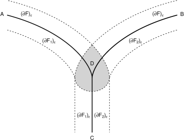
Figure 3: The shaded set illustrates condition (15). The curve ADC is part of $\partial F_{1}$, BDC is part of $\partial F_{2}$, while ADB is part of $\partial F$.

Lemma 7.

Suppose $F_{1},F_{2}$ yield a normal decomposition of $F=F_{1}\cup F_{2}$. Then

$$\Theta_{d-1}(C,\{(x,u)\in\operatorname{\rm Nor}(C):x\in\partial F\cap\partial F_{1}\cap\partial F_{2}\})=0.$$ (16)

Moreover, we have

$$\frac{1}{\varepsilon}\mu_{d}\left((\partial F_{1}\triangle\partial F_{2})_{\varepsilon}\cap(\partial F_{1}\cap\partial F_{2})_{\varepsilon}\right)\to 0$$ (17)

and

$$\frac{1}{\varepsilon}\mu_{d}\left(((\partial F_{1})_{\varepsilon}\cap(\partial F_{2})_{\varepsilon})\setminus(\partial F_{1}\cap\partial F_{2})_{\varepsilon}\right)\to 0,$$ (18)

as $\varepsilon\to 0$.

Proof.

The first assertion, (16), is a direct consequence of (15) and the Steiner formula.

Since $\partial F_{1}\triangle\partial F_{2}\subseteq\partial F,$ we have $(\partial F_{1}\triangle\partial F_{2})_{\varepsilon}\subseteq(\partial F)_{\varepsilon}$ and at the same time

$$(\partial F_{1}\cap\partial F_{2})_{\varepsilon}\subseteq(\partial F_{1})_{\varepsilon}\cap(\partial F_{2})_{\varepsilon}.$$

Therefore,

$$(\partial F_{1}\triangle\partial F_{2})_{\varepsilon}\cap(\partial F_{1}\cap\partial F_{2})_{\varepsilon}\subseteq(\partial F)_{\varepsilon}\cap(\partial F_{1})_{\varepsilon}\cap(\partial F_{2})_{\varepsilon},$$

and (17) follows from condition (15).

With respect to (18),

$$z\in((\partial F_{1})_{\varepsilon}\cap(\partial F_{2})_{\varepsilon})\setminus(\partial F_{1}\cap\partial F_{2})_{\varepsilon}$$

implies that the distances $d_{\partial F_{1}}(z),d_{\partial F_{2}}(z)$ do not exceed $\varepsilon$, but $d_{\partial F_{1}\cap\partial F_{2}}(z)>\varepsilon$. Therefore $z$ is on a distance smaller than or equal $\varepsilon$ not from $\partial F_{1}\cap\partial F_{2}$, but from $\partial F_{1}\triangle\partial F_{2}$, that is, from $\partial F$. Hence

$$((\partial F_{1})_{\varepsilon}\cap(\partial F_{2})_{\varepsilon})\setminus(\partial F_{1}\cap\partial F_{2})_{\varepsilon}\subseteq(\partial F)_{\varepsilon}\cap(\partial F_{1})_{\varepsilon}\cap(\partial F_{2})_{\varepsilon}$$

and (18) follows, again from (15). ∎

We now discuss the normal cylinders of the sets involved. Apparently, this reduces to a discussion of the corresponding normal bundles. The normal bundle $\operatorname{\rm Nor}(C)$ of $C$ can be embedded as a subset into the union of the normal bundles $\operatorname{\rm Nor}(\partial F_{i})$, $i=1,2$. In fact, any $(x,u)\in\operatorname{\rm Nor}(C)$ comes from a point $z\notin C$ which (uniquely) projects onto $x\in C$. If $x\in\partial F_{1}$, then $x$ is also the projection of $z$ onto $\partial F_{1}$ and hence $(x,u)\in\operatorname{\rm Nor}(F_{1})$. We similarly argue if $x\in\partial F_{2}$.

In order to embed also $\operatorname{\rm Nor}(\partial F_{1})$ into $\operatorname{\rm Nor}(C)$, we have to neglect pairs $(x_{1},u)$ from $\operatorname{\rm Nor}(\partial F_{1})$ for which $u$ is not a normal at $x$ in $C$. For such a pair $(x_{1},u)\in\operatorname{\rm Nor}(\partial F_{1})$, there exists small enough $\varepsilon$, such that all $z=x_{1}+tu,t\leq\varepsilon,$ project onto $x_{1}$. Since $\partial F_{1}\subseteq C$, there is a point $x_{2}\in C$ with

$$\|z-x_{2}\|=\inf_{x\in C}\|z-x\|\leq\inf_{x\in\partial F_{1}}\|z-x\|=\|z-x_{1}\|,$$

and therefore all points $z=x_{1}+tu,t\leq\varepsilon,$ are in $C_{\varepsilon}$. However, $x_{2}$ has to be different from $x_{1}$. Otherwise, we would have $(z-x_{2})/\|z-x_{2}\|=u$ and $(x_{1},u)\in\operatorname{\rm Nor}(C)$, a contradiction. Therefore, we obtain $z\in(\partial F_{1})_{\varepsilon}\cap(\partial F_{2})_{\varepsilon}\setminus C_{\varepsilon}$. Applying the local magnification map $\tau_{\varepsilon}^{(1)}$ to this set and using (18) and the Steiner formula, we deduce that

$$\Theta_{d-1}(\partial F_{1},\operatorname{\rm Nor}(\partial F_{1})\setminus\operatorname{\rm Nor}(C))=0,$$

which shows that we can embed $\Sigma(\partial F_{1})$ into $\Sigma(C)$, up to a set of measure 0. In the same way, we can embed $\operatorname{\rm Nor}(\partial F_{2})$ into $\operatorname{\rm Nor}(C)$.

Therefore, we identify now the normal cylinders $\Sigma(C)$ and $\Sigma(F_{1})\cup\Sigma(F_{2})$. If $B_{i}$ denotes the derivative of $F_{i}(\varepsilon)$ at $F_{i}$, $i=1,2$, the positive part $B_{i}^{+}$ and the reflection $R(B_{i}^{-})$ of its negative part $B_{i}^{-}$ can be seen as subsets of $\Sigma(\partial F_{i})$, as we have explained before Theorem 6 and therefore also as subsets of $\Sigma(C)$, for $i=1,2$. Since we can also embed the normal cylinders $\Sigma(F)$ of $F$ and $\Sigma(F_{i})$ of $F_{i}$, $i=1,2$, into $\Sigma=\Sigma(C)$ by the mapping $(t,x,u)\mapsto(t,x,u)$, for $t\geq 0$, and by the reflection $R:(t,x,u)\mapsto(-t,x,-u)$, for $t<0$, we can extend the measures $M_{F}$ and $M_{F_{i}},i=1,2$, to $\Sigma(C)$, in the obvious way. We denote by $M_{F}^{+},M_{F}^{-}$ the restrictions of $M_{F}$ to $\Sigma^{+}(F)$ respectively $\Sigma^{-}(F)$ and we use similar notations for the measures $M_{F_{i}}$, $i=1,2$.

Lemma 8.

Suppose $F_{1},F_{2}$ yield a normal decomposition of $F=F_{1}\cup F_{2}$. Then

$$M_{C}=M_{F}^{+}+M_{F_{1}}^{-}\circ R+M_{F_{2}}^{-}\circ R.$$ (19)

Proof.

The assertion follows from a corresponding decomposition of the support measures,

$$\Theta_{d-1}(C,\cdot) =\Theta_{d-1}(F,\cdot)+\Theta_{d-1}(F_{1}^{\ast},\cdot)+\Theta_{d-1}(F_{2}^{\ast},\cdot)$$

which is a consequence of (6) and (12), together with (16). ∎

We now formulate our main result in this section.

Theorem 9.

Let $F_{1}(\varepsilon),F_{2}(\varepsilon),0\leq\varepsilon\leq 1,$ be two families of nonempty compact sets such that, for each fixed $\varepsilon>0$, the sets $F_{1}(\varepsilon)$ and $F_{2}(\varepsilon)$ are pairwise disjoint, and let $F(\varepsilon)=F_{1}(\varepsilon)\cup F_{2}(\varepsilon)$. Assume that $F_{1}=F_{1}(0)$ and $F_{2}=F_{2}(0)$ provide a normal decomposition of $F=F(0)=F_{1}\cup F_{2}$.

If the families $F_{i}(\varepsilon)$ are differentiable at $F_{i}$ with derivative $B_{i}$, $i=1,2$, then

$$C(\varepsilon)=F(\varepsilon)\triangle F$$

is differentiable at

$$C=\partial F_{1}\cup\partial F_{2}$$

with derivative $B=\tilde{B}_{1}\cup\tilde{B}_{2}$ where

$$\tilde{B}_{i}=\left\{{R(B_{i}^{-})\setminus B_{j}^{+}{\text{\ }on\ }\Sigma(C_{ij}),{\text{\ }for\ }j\not=i,}\atop{B_{i}^{+}\cup R(B_{i}^{-}){\text{ \ otherwise.}}}\right.$$

Proof.

We start with the essential boundedness condition. Since the families $F_{i}(\varepsilon)\triangle F_{i}$ are essentially bounded, we may assume that there is a $T$ such that

$$F_{i}(\varepsilon)\triangle F_{i}\subset(\partial F_{i})_{T\varepsilon},\quad i=1,2.$$

We may also put $T=1$. It is then easy to see that

$$F(\varepsilon)\triangle F\subset C_{\varepsilon},$$

hence $C(\varepsilon)$ is essentially bounded.

In order to show that $F(\varepsilon)\triangle F$ is differentiable at $C$ with derivative $B$, it remains to show that

$$M_{C}(\tau_{\varepsilon}(F(\varepsilon)\triangle F)\triangle B)\to 0,$$

as $\varepsilon\to 0$. Observe that here $\tau_{\varepsilon}$ is the magnification map belonging to $C$. Later, we will also use the magnification map $\tau_{\varepsilon}^{(i)}$ belonging to $\partial F_{i}$, $i=1,2$. For $z\notin C\cup S_{C}\cup S_{\partial F_{1}}\cup S_{\partial F_{2}}$, we then have $\tau_{\varepsilon}(z)=\tau_{\varepsilon}^{(i)}(z)$, for some $i$ (possibly for both). We now use (19) and discuss the effects of the different summands of $M_{C}$ to the set $\tau_{\varepsilon}(F(\varepsilon)\triangle F)\triangle B$ separately.

Since $M_{F}^{+}$ is concentrated on $[0,\infty)\times\operatorname{\rm Nor}(F)$ (notice that we can use $\operatorname{\rm Nor}(F)$ instead of $\operatorname{\rm Nor}_{e}(F)$ here), we can decompose $M_{F}^{+}$ into a sum

$$M_{F}^{+}=M^{(1)}+M^{(2)},$$

where

$$M^{(i)}=\mu_{1}^{+}\otimes\left[\Theta_{d-1}(F_{i},\cdot)\,\rule{0.28453pt}{6.82881pt}\rule{6.82881pt}{0.28453pt}\,\left(\operatorname{\rm Nor}(F_{i})\cap\operatorname{\rm Nor}(F)\right)\right],\ i=1,2.$$

Here, $\mu_{1}^{+}$ is the Lebesgue measure on $[0,\infty)$ and $\rho\,\rule{0.28453pt}{6.82881pt}\rule{6.82881pt}{0.28453pt}\,A$ denotes the restriction of the measure $\rho$ to the set $A$. Using this decomposition and the facts that

$$\tau_{\varepsilon}(F(\varepsilon)\triangle F)\triangle B\subset[\tau_{\varepsilon}(F(\varepsilon)\setminus F)\triangle B]\cup\tau_{\varepsilon}(F)$$

and $M_{F}^{+}(\tau_{\varepsilon}(F))=0,$ we first obtain

$$M_{F}^{+}(\tau_{\varepsilon}(F(\varepsilon)\triangle F)\triangle B) \leq M_{F}^{+}(\tau_{\varepsilon}(F(\varepsilon)\setminus F)\triangle B)$$

$$=\sum_{i=1}^{2}M^{(i)}(\tau_{\varepsilon}(F(\varepsilon)\setminus F)\triangle B).$$

On $[0,\infty)\times(\operatorname{\rm Nor}(F_{1})\cap\operatorname{\rm Nor}(F))$, we have

$$\tau_{\varepsilon}(F(\varepsilon)\setminus F) =\tau_{\varepsilon}^{(1)}((F(\varepsilon)\setminus F)\cap(\partial F_{1})_{\varepsilon})$$

$$=\tau_{\varepsilon}^{(1)}(F_{1}(\varepsilon)\setminus F_{1})\cup\tau_{\varepsilon}^{(1)}((F_{2}(\varepsilon)\setminus F_{1})\cap(\partial F_{1})_{\varepsilon}),$$

hence

$$M^{(1)} (\tau_{\varepsilon}(F(\varepsilon)\setminus F)\triangle B)$$ (20)

$$\leq M^{(1)}(\tau_{\varepsilon}^{(1)}(F_{1}(\varepsilon)\setminus F_{1})\triangle B)+M^{(1)}(\tau_{\varepsilon}^{(1)}((F_{2}(\varepsilon)\setminus F_{1})\cap(\partial F_{1})_{\varepsilon})).\quad\quad$$ (21)

Moreover,

$$M^{(1)}(B_{2}^{+})=M^{(1)}(R(B_{2}^{-}))=M^{(1)}(B_{1}^{-})=M^{(1)}(R(B_{1}^{-}))=0$$

(the latter fact arises, since $\operatorname{\rm Nor}(F_{1})$ and $R(B_{1}^{-})$ are disjoint subsets of $\operatorname{\rm Nor}(C)$). Therefore,

$$M^{(1)}(\tau_{\varepsilon}^{(1)}(F_{1}(\varepsilon)\setminus F_{1})\triangle B) =M^{(1)}(\tau_{\varepsilon}^{(1)}(F_{1}(\varepsilon)\setminus F_{1})\triangle B_{1}^{+})$$

$$=M^{(1)}(\tau_{\varepsilon}^{(1)}(F_{1}(\varepsilon)\triangle F_{1})\triangle B_{1}^{+})$$

$$=M^{(1)}(\tau_{\varepsilon}^{(1)}(F_{1}(\varepsilon)\triangle F_{1})\triangle B_{1}).$$

Since $M^{(1)}\leq M_{F_{1}}$, we get

$$M^{(1)}(\tau_{\varepsilon}^{(1)}(F_{1}(\varepsilon)\setminus F_{1})\triangle B)\leq M_{F_{1}}(\tau_{\varepsilon}^{(1)}(F_{1}(\varepsilon)\triangle F_{1})\triangle B_{1})\to 0,$$ (22)

as $\varepsilon\to 0$, due to the differentiability of $F_{1}(\varepsilon)$.

Furthermore, we notice that points $z$ in $(F_{2}(\varepsilon)\setminus F_{1})\cap(\partial F_{1})_{\varepsilon}$ which project onto $\partial F_{1}$ must lie in $(\partial F_{1}\setminus\partial F_{2})_{\varepsilon}\cap(\partial F_{1}\cap\partial F_{2})_{\varepsilon}$, and so

$$M^{(1)} (\tau_{\varepsilon}^{(1)}((F_{2}(\varepsilon)\setminus F_{1})\cap(\partial F_{1})_{\varepsilon}))$$

$$\leq M^{(1)}(\tau_{\varepsilon}^{(1)}((\partial F_{1}\setminus\partial F_{2})_{\varepsilon}\cap(\partial F_{1}\cap\partial F_{2})_{\varepsilon})).$$

The local Steiner formula (2) shows that

$$\frac{1}{\varepsilon} \mu_{d}((\partial F_{1}\setminus\partial F_{2})_{\varepsilon}\cap(\partial F_{1}\cap\partial F_{2})_{\varepsilon})$$

$$\quad=M^{(1)}(\tau_{\varepsilon}^{(1)}((\partial F_{1}\setminus\partial F_{2})_{\varepsilon}\cap(\partial F_{1}\cap\partial F_{2})_{\varepsilon}))+o(\varepsilon).$$

Therefore, (17) implies

$$M^{(1)}(\tau_{\varepsilon}^{(1)}((\partial F_{1}\setminus\partial F_{2})_{\varepsilon}\cap(\partial F_{1}\cap\partial F_{2})_{\varepsilon}))\to 0,$$ (23)

as $\varepsilon\to 0$. Combining (20), (22) and (23) gives

$$M^{(1)}(\tau_{\varepsilon}(F(\varepsilon)\setminus F)\triangle B)\to 0.$$

In the same way, we get

$$M^{(2)}(\tau_{\varepsilon}(F(\varepsilon)\setminus F)\triangle B)\to 0,$$

hence

$$M_{F}^{+}(\tau_{\varepsilon}(F(\varepsilon)\triangle F)\triangle B)\to 0.$$ (24)

Now, we consider

$$(M_{F_{1}}^{-}\circ R)(\tau_{\varepsilon}(F(\varepsilon)\triangle F)\triangle B).$$

Observe that $\tilde{M}_{F_{1}}=M_{F_{1}}^{-}\circ R$ is a measure on $R(\Sigma^{-}(F_{1}))$. On this set, we have

$$\tau_{\varepsilon}(F(\varepsilon)\triangle F) =\tau_{\varepsilon}^{(1)}(F_{1}\setminus F(\varepsilon))$$

$$=[\tau_{\varepsilon}^{(1)}(F_{1}\setminus F(\varepsilon))\cap\Sigma(F)]\cup[\tau_{\varepsilon}^{(1)}(F_{1}\setminus F(\varepsilon))\cap\Sigma_{12}],$$

here $\Sigma_{12}=[0,\infty)\times(\operatorname{\rm Nor}(\partial F_{1})\setminus\operatorname{\rm Nor}(F))$ is the normal cylinder of $C_{12}$ in relative interior points of $C_{12}$ and with normals $u$ pointing into the interior of $F_{1}$. Notice that the sets $\tau_{\varepsilon}^{(1)}((F_{1}\setminus F(\varepsilon))\cap\Sigma(F))$ and $\tau_{\varepsilon}^{(1)}((F_{1}\setminus F(\varepsilon))\cap\Sigma_{12})$ live on different parts of the cylinder $\Sigma(C)$. Therefore,

$$\tilde{M}_{F_{1}} (\tau_{\varepsilon}(F(\varepsilon)\triangle F)\triangle B)=\tilde{M}_{F_{1}}((\tau_{\varepsilon}^{(1)}(F_{1}\setminus F(\varepsilon))\cap\Sigma(F))\triangle(R(B_{1}^{-})\cap\Sigma(F)))$$

$$\quad+\tilde{M}_{F_{1}}((\tau_{\varepsilon}^{(1)}(F_{1}\setminus F(\varepsilon))\cap\Sigma_{12})\triangle((B_{2}^{+}\cup R(B_{1}^{-}))\cap\Sigma_{12}))$$

$$=\tilde{M}^{(1)}(\tau_{\varepsilon}^{(1)}(F_{1}\setminus F(\varepsilon))\triangle R(B_{1}^{-}))$$ (25)

$$\quad+\tilde{M}^{(2)}(\tau_{\varepsilon}^{(1)}(F_{1}\setminus F(\varepsilon))\triangle(B_{2}^{+}\cup R(B_{1}^{-}))).$$

Here, $\tilde{M}^{(1)}$ denotes the restriction of $\tilde{M}_{F_{1}}$ to $\Sigma(F)$ and $\tilde{M}^{(2)}$ is the restriction to $\Sigma_{12}$.

For the first summand, we use

$$\tau_{\varepsilon}^{(1)}(F_{1}\setminus F(\varepsilon))=\tau_{\varepsilon}^{(1)}(F_{1}\setminus F_{1}(\varepsilon))\setminus\tau_{\varepsilon}^{(1)}(F_{1}\cap F_{2}(\varepsilon))$$

and

$$\tilde{M}^{(1)}(\tau_{\varepsilon}^{(1)} (F_{1}\setminus F_{1}(\varepsilon))\triangle R(B_{1}^{-}))\to 0,$$

since $F_{1}(\varepsilon)$ is differentiable at $F_{1}$. Also

$$\tilde{M}^{(1)}(\tau_{\varepsilon}^{(1)}(F_{1}\cap F_{2}(\varepsilon)))\to 0.$$ (26)

In fact, the Steiner formula (2) shows that

$$\tilde{M}^{(1)}(\tau_{\varepsilon}^{(1)}(F_{1}\cap F_{2}(\varepsilon)))=\frac{1}{\varepsilon}\mu_{d}((\partial F_{1})_{\varepsilon}\cap(F_{1}\cap F_{2}(\varepsilon)))+o(\varepsilon).$$

Points $z\in(\partial F_{1})_{\varepsilon}\cap(F_{1}\cap F_{2}(\varepsilon))$ which project onto $\partial F$ lie in $(\partial F_{1})_{\varepsilon}\cap(\partial F_{2})_{\varepsilon}\cap(\partial F)_{\varepsilon}$. Hence, the assertion follows from (15).

Together we get

$$\tilde{M}^{(1)}(\tau_{\varepsilon}^{(1)}(F_{1}\setminus F(\varepsilon))\triangle R(B_{1}^{-}))\to 0.$$ (27)

For the second summand in (5), we similarly have

$$\tau_{\varepsilon}^{(1)}(F_{1}\setminus F(\varepsilon))=\tau_{\varepsilon}^{(1)}(F_{1}\setminus F_{1}(\varepsilon))\setminus\tau_{\varepsilon}^{(1)}(F_{1}\cap F_{2}(\varepsilon))$$

with

$$\tilde{M}^{(2)}(\tau_{\varepsilon}^{(1)}(F_{1}\setminus F_{1}(\varepsilon))\triangle R(B_{1}^{-}))\to 0,$$

again by the differentiability of $F_{1}(\varepsilon)$. On the other hand,

$$\tilde{M}^{(2)}(\tau_{\varepsilon}^{(1)}(F_{1}\cap F_{2}(\varepsilon)))=\tilde{M}_{F_{1}}(\tau_{\varepsilon}^{(1)}((F_{1}\cap F_{2}(\varepsilon))\cap\Sigma_{12}))$$

$$=M_{F_{2}}^{+}(\tau_{\varepsilon}^{(2)}(F_{1}\cap F_{2}(\varepsilon))\cap\Sigma_{12})-\tilde{M}_{F_{1}}(\tau_{\varepsilon}^{(1)}(F_{1}\cap F_{2}(\varepsilon))\cap\Sigma(F)),$$

taking into account the points in $F_{1}\cap F_{2}(\varepsilon)$ which project onto $\partial F$ and not onto $C_{12}$. Here,

$$M_{F_{2}}^{+}((\tau_{\varepsilon}^{(2)}(F_{1}\cap F_{2}(\varepsilon))\cap\Sigma_{12})\triangle(B_{2}^{+}\cap\Sigma_{12}))\to 0,$$

by the differentiability of $F_{2}(\varepsilon)$ and the term

$$\tilde{M}_{F_{1}}(\tau_{\varepsilon}^{(1)}(F_{1}\cap F_{2}(\varepsilon))\cap\Sigma(F))$$

converges to 0 by our condition (15), as we have seen in (26). Hence,

$$\tilde{M}^{(2)}(\tau_{\varepsilon}^{(1)}(F_{1}\cap F_{2}(\varepsilon))\triangle B_{2}^{+})\to 0.$$

Together we obtain

$$\tilde{M}^{(2)}(\tau_{\varepsilon}^{(1)}(F_{1}\setminus F(\varepsilon))\triangle(R(B_{1}^{-})\setminus B_{2}^{+}))$$ (28)

$$\ =\tilde{M}^{(2)}(\tau_{\varepsilon}^{(1)}(F_{1})\setminus F_{1}(\varepsilon))\triangle\tau_{\varepsilon}^{(1)}(F_{1}\cap F_{2}(\varepsilon))\triangle(R(B_{1}^{-})\triangle B_{2}^{+}))$$ (29)

$$\ \leq\tilde{M}^{(2)}(\tau_{\varepsilon}^{(1)}(F_{1})\setminus F_{1}(\varepsilon))\triangle R(B_{1}^{-}))+\tilde{M}^{(2)}(\tau_{\varepsilon}^{(1)}(F_{1}\cap F_{2}(\varepsilon))\triangle B_{2}^{+})$$ (30)

$$\ \to 0.$$ (31)

From (27) and (28), we arrive at

$$(M_{F_{1}}^{-}\circ R) (\tau_{\varepsilon}(F\triangle F(\varepsilon)))\triangle B)\to 0.$$ (32)

In the same manner, we get

$$(M_{F_{2}}^{-}\circ R) (\tau_{\varepsilon}(F\triangle F(\varepsilon)))\triangle B)\to 0.$$ (33)

Combining (24), (32) and (33), we obtain the asserted differentiability. ∎

6 Parallel sets

We now discuss some particular classes of set-valued mappings which are differentiable, the subgraphs and the local or global parallel sets.

Let $F=F(0)$ be a solid set and $h_{\varepsilon},0\leq\varepsilon\leq 1$, a family of nonnegative measurable functions on $\operatorname{\rm Nor}(F)$ (with $h_{0}=0$). As in [9], we call

$$h_{\varepsilon,{\rm sub}} =\{z=x+tu:(x,u)\in\operatorname{\rm Nor}(F),0<t\leq h_{\varepsilon}(x,u)\wedge r(x,u)\}$$

the subgraph of $h_{\varepsilon}$. We assume that the following two conditions hold:

1. For each $(x,u)\in\operatorname{\rm Nor}(F)$, $\varepsilon\to h_{\varepsilon}(x,u)$ is differentiable at $\varepsilon=0$ with derivative $g(x,u)$. Thus

   $$\frac{h_{\varepsilon}(x,u)}{\varepsilon}\to g(x,u),\quad\varepsilon\to 0.$$

2. There is a $\delta>0$, such that the function $\max_{0<\varepsilon\leq\delta}\frac{h_{\varepsilon}}{\varepsilon}$ is bounded and integrable with respect to $\Theta_{d-1}(F,\cdot)$. Hence,

   $$\max_{0<\varepsilon\leq\delta}\frac{h_{\varepsilon}(x,u)}{\varepsilon}\leq T,$$ (34)

   for some $T>0$ and

   $$\int_{\operatorname{\rm Nor}(F)}\max_{0<\varepsilon\leq\delta}\frac{h_{\varepsilon}(x,u)}{\varepsilon}\,\Theta_{d-1}(F,d(x,u))<\infty.$$

Theorem 10.

Let $F$ be solid and let $h_{\varepsilon},0\leq\varepsilon\leq 1$, be a family of nonnegative measurable functions on $\operatorname{\rm Nor}(F)$ satisfying conditions (a) and (b). Then, $A(\varepsilon)=h_{\varepsilon,{\rm sub}}$ is differentiable at $\partial F$ and the derivative is

$$B=\{(t,x,u):0<t\leq g(x,u),(x,u)\in\operatorname{\rm Nor}(F)\}.$$

Proof.

We first show that $A(\varepsilon)$ is essentially bounded. Let $\delta$ be given as in (b) and let $T$ be the bound from (34). Suppose $\varepsilon\leq\delta$. Then,

$$\frac{1}{\varepsilon}\mu_{d}(A(\varepsilon)\cap({\mathbb{R}}^{d}\setminus(\partial F)_{\varepsilon T}))$$

$$\ =\frac{1}{\varepsilon}\mu_{d}(\{z=x+tu:(x,u)\in\operatorname{\rm Nor}(F),\varepsilon T<t\leq h_{\varepsilon}(x,u)\wedge r(x,u)\}$$

equals $0$, because condition (b) implies that the set here is empty. Hence, $A(\varepsilon)$ is essentially bounded.

With respect to the differentiability, we observe that

$$M(\tau_{\varepsilon} (A(\varepsilon))\triangle B)$$

$$\ =\int_{\operatorname{\rm Nor}(F)}\int_{0}^{\infty}{\bf 1}(\{0<t\leq\frac{h_{\varepsilon}(x,u)\wedge r(x,u)}{\varepsilon}\}\triangle\{0<t\leq g(x,u)\})$$

$$\quad\quad\times dt\,\Theta_{d-1}(F,d(x,u))$$

$$\ =\int_{\operatorname{\rm Nor}(F)}\left|\frac{h_{\varepsilon}(x,u)\wedge r(x,u)}{\varepsilon}-g(x,u)\right|\Theta_{d-1}(F,d(x,u)).$$

Since $r(x,u)>0$, for $(x,u)\in\operatorname{\rm Nor}(F)$, the integrand converges to $0$ pointwisely. Also,

$$\left|\frac{h_{\varepsilon}(x,u)\wedge r(x,u)}{\varepsilon}-g(x,u)\right| \leq\frac{h_{\varepsilon}(x,u)\wedge r(x,u)}{\varepsilon}+g(x,u)$$

$$\leq 2\max_{0<\varepsilon\leq\delta}\frac{h_{\varepsilon}(x,u)}{\varepsilon},$$

and the latter function is integrable with respect to $\Theta_{d-1}(F,\cdot)$, by (b). The Dominated Convergence Theorem thus implies

$$M(F(\varepsilon)\triangle B)\to 0,\quad\varepsilon\to 0.$$

This completes the proof of the theorem. ∎

We remark that we could also start with a family $\tilde{h}_{\varepsilon},0<\varepsilon\leq 1$, of functions on $\partial F$ and put $h_{\varepsilon}(x,u)=\tilde{h}_{\varepsilon}(x),(x,u)\in\operatorname{\rm Nor}(F),$ or with a family $\bar{h}_{\varepsilon},0<\varepsilon\leq 1$, of functions on $S^{d-1}$ and put $h_{\varepsilon}(x,u)=\bar{h}_{\varepsilon}(u),(x,u)\in\operatorname{\rm Nor}(F)$.

As a particular case, $h_{\varepsilon}=\varepsilon g$ and the function $g$ could be given by the support function $h_{K}$ of a convex body $K$ with $0\in K$,

$$g(x,u)=h_{K}(u),\quad(x,u)\in\operatorname{\rm Nor}(F).$$

The subgraph $h_{\varepsilon,{\rm sub}}$, obtained in this case, is different in general from the outer parallel strip $F+\varepsilon K\setminus F$. A differentiability result for outer parallel sets $F+\varepsilon K$, $\varepsilon\to 0$, under different conditions, is discussed in the final Section 6. However, if $K$ is the unit ball $B^{d}$ and

$$h_{\varepsilon}(x,u)=\varepsilon h_{B^{d}}(u)=\varepsilon,$$

then $h_{\varepsilon,{\rm sub}}=F+\varepsilon B^{d}\setminus F$, as can be easily seen.

A case of particular interest arises, if we choose, in the previous discussion, $h(x,u)=r(x,u)\wedge 1,(x,u)\in\operatorname{\rm Nor}(F)$. If we define, for $\varepsilon>0$, the local parallel set $F_{\varepsilon,{\rm loc}}$ of $F$ as

$$F_{\varepsilon,{\rm loc}}=F\cup\{z=x+tu:(x,u)\in\operatorname{\rm Nor}F,0<t\leq\varepsilon r(x,u)\wedge\varepsilon\},$$

then $F_{\varepsilon,{\rm loc}}$ is the subgraph of $\varepsilon h$. The derivative of $\varepsilon h$ is $r\wedge 1$, hence in the above proof we have

$$M(\tau_{\varepsilon} (A(\varepsilon))\triangle B)$$

$$\ =\int_{\operatorname{\rm Nor}(F)}\left|\frac{h_{\varepsilon}(x,u)\wedge r(x,u)}{\varepsilon}-g(x,u)\right|\Theta_{d-1}(F,d(x,u))$$

$$\ =\int_{\operatorname{\rm Nor}(F)}\left|\frac{\varepsilon(r(x,u)\wedge 1)\wedge r(x,u)}{\varepsilon}-(r(x,u)\wedge 1)\right|\Theta_{d-1}(F,d(x,u))$$

$$\ =0,$$

for $\varepsilon\leq 1$. Condition (b) is satisfied automatically since $r\wedge 1$ is bounded and integrable with respect to $\Theta_{d-1}(F,\cdot)$ by (1). Hence, we obtain the following result.

Corollary 11.

Let $F$ be a solid set. Then the local parallel set $F_{\varepsilon,{\rm loc}}$, $0<\varepsilon\leq 1$, is differentiable at $F$ with derivative

$$B=\{(t,x,u):(x,u)\in\operatorname{\rm Nor}(F),0\leq t\leq r(x,u)\wedge 1\}.$$

As a consequence, the parallel set $F+\varepsilon B^{d}$ of a convex body $F$ is differentiable, as we already mentioned above. This is a special case of a result in [9] which shows differentiability of $F+\varepsilon K$, for general convex bodies $F,K$. Our next goal is to extend the latter result to solid sets $F$

For this purpose, we consider the support function $h_{K}$ of $K$; it can be seen as a continuous function on $S^{d-1}$. We define a function $h_{K,F}$ on $\operatorname{\rm Nor}(F)$ by

$$h_{K,F}(x,u)=h_{K}(u),\quad(x,u)\in\operatorname{\rm Nor}(F),$$

and put

$$(h_{K,F})_{\rm sub} =\{(t,x,u)\in\Sigma:0<t\leq h_{K}(u)\}$$

$$\hskip 56.9055pt\cup\{(t,x,u)\in\Sigma:h_{K}(u)\leq t<0\}.$$

Notice, that we do not require $0\in K$ here. This is another difference to the discussion of subgraphs above.

In the following theorem, we assume, in addition, that the support measure $\Theta_{d-1}(F,\cdot)$ is finite (this follows, for example, if $\partial F$ has finite $(d-1)$-st Hausdorff measure) and that the set of boundary points of $F$ which are not normal has ${\cal H}^{d-1}$-measure $0$. Here, a point $x\in\partial F$ is called normal, if there is some ball $B\subset F$ with $x\in B$.

Theorem 12.

Let $F$ be a solid set with $\Theta_{d-1}(F,\operatorname{\rm Nor}(F))<\infty$ and such that

$${\cal H}^{d-1}(\{x\in\partial F:x{\rm\ not\ normal}\})=0.$$

Let $K$ be a convex body. Then $F(\varepsilon)=F+\varepsilon K,0\leq\varepsilon\leq 1$, is differentiable at $F$, and we have

$$\frac{d}{d\varepsilon}F(\varepsilon)=(h_{K,F})_{\rm sub}.$$

Proof.

For $k=1,2,...$, let $\partial F_{(k)}$ be the set of all regular boundary points $x$ of $F$ for which there is a ball of radius $\geq 1/k$ inside $F$ with $x\in B$. Let $u=u(x)$ be the corresponding (outer) normal. Let $\Sigma_{(k)}\subset\Sigma$ be the part of the normal cylinder which belongs to points $(x,u(x)),x\in\partial F_{(k)}$. We fix $k$ and choose $\varepsilon$ small enough such that $\varepsilon K\subset\frac{1}{k}B^{d}$. Then, we consider

$$M([\tau_{\varepsilon}(F(\varepsilon)\triangle F)\triangle(h_{K,F})_{\rm sub}]\cap\Sigma_{(k)}).$$

For $x\in\partial F_{(k)}$ (with normal $u$), we have $B(1/k)\subset F\subset H(x,u)$, where $B(1/k)$ is the ball of radius $1/k$ touching $F$ at $x$ from inside. $H(x,u)$ is the closure of the complement ${\mathbb{R}}^{d}\setminus C$, where $C$ is the ball of radius $r(x,u)$ touching $F$ in $x$ from outside. If the reach $r(x,u)$ is $\infty$, then $H(x,u)$ is the closed halfspace with outer normal $u$ and containing $x$ in the boundary. We divide $\Sigma_{(k)}$ further into the sets $\Sigma_{(k)}^{+}$ and $\Sigma_{(k)}^{-}$ according to the case where $h_{K,F}(x,u)\geq 0$, respectively $h_{K,F}(x,u)<0$.

Since $\varepsilon K\subset\frac{1}{k}B^{d}$, we have

$$[\tau_{\varepsilon}(F(\varepsilon)\triangle F)\triangle(h_{K,F})_{\rm sub}]\cap\Sigma_{(k)}^{+}=[\tau_{\varepsilon}(F(\varepsilon)\setminus F)\triangle(h_{K,F})_{\rm sub}]\cap\Sigma_{(k)}^{+}$$

and

$$\tau_{\varepsilon}(F(\varepsilon)\setminus F)\cap\Sigma_{(k)}^{+}=\{(\frac{t}{\varepsilon},x,u):0<t\leq g_{\varepsilon K}(x,u)\},$$

where $g_{\varepsilon K}(x,u)$ is the distance from $x$ to $\partial F(\varepsilon)$ in direction $u$. For $F=H(x,u)$ this distance would be $\varepsilon h_{K}(u)$, for $F=B(1/k)$ the distance is $\geq\varepsilon h_{K}(u)+\sqrt{(1/k)^{2}-\varepsilon^{2}(a(u)^{2}-h_{K}^{2}(u))}-1/k$, where $a(u)$ is the maximal length of a point $y\in K$ with $\langle y,u\rangle=h_{K}(u)$. Hence

$$\varepsilon h_{K}(u)+\sqrt{\frac{1}{k^{2}}-\varepsilon^{2}(a(u)^{2}-h_{K}^{2}(u))}-\frac{1}{k}\leq g_{\varepsilon K}(x,u)\leq\varepsilon h_{K}(u).$$

We obtain that

$$[ \tau_{\varepsilon}(F(\varepsilon)\setminus F)\triangle(h_{K,F})_{\rm sub}]\cap\Sigma_{(k)}$$

$$\subset\left\{(t,x,u):h_{K}(u)+\frac{1}{\varepsilon}\left(\sqrt{\frac{1}{k^{2}}-\varepsilon^{2}(a(u)^{2}-h_{K}^{2}(u))}-\frac{1}{k}\right)\leq t\leq h_{K}(u)\right\}.$$

Since

$$\lim_{\varepsilon\to 0}\frac{1}{\varepsilon}\left(\sqrt{\frac{1}{k^{2}}-\varepsilon^{2}(a(u)^{2}-h_{K}^{2}(u))}-\frac{1}{k}\right)=0,$$

we see that

$$M([\tau_{\varepsilon}(F(\varepsilon)\setminus F)\triangle(h_{K,F})_{\rm sub}]\cap\Sigma_{(k)}^{+})\to 0.$$

In a totally analogous way, we obtain that

$$[\tau_{\varepsilon}(F(\varepsilon)\triangle F)\triangle(h_{K,F})_{\rm sub}]\cap\Sigma_{(k)}^{-}=[\tau_{\varepsilon}(F\setminus F(\varepsilon))\triangle(h_{K,F})_{\rm sub}]\cap\Sigma_{(k)}^{-}$$

and

$$M([\tau_{\varepsilon}(F\setminus F(\varepsilon))\triangle(h_{K,F})_{\rm sub}]\cap\Sigma_{(k)}^{-})\to 0.$$

Hence,

$$M([\tau_{\varepsilon}(F\triangle F(\varepsilon))\triangle(h_{K,F})_{\rm sub}]\cap\Sigma_{(k)})\to 0,$$

for each $k$, and therefore also

$$M(\tau_{\varepsilon}(F(\varepsilon)\setminus F)\triangle(h_{K,F})_{\rm sub})\to 0,$$

as $\varepsilon\to 0$. ∎

The conditions on $F$ are fulfilled, in particular, if $F$ is a convex body with interior points, the assumption on the normal boundary points then follows from [15, Th. 2.5.5]. As a corollary, we thus get the following result which was mentioned in [9] (with reference to [15], but without further details).

Corollary 13.

Let $F$ and $K$ be convex bodies und such that $F$ has interior points. Then $F(\varepsilon)=F+\varepsilon K,0\leq\varepsilon\leq 1$, is differentiable at $F$, and we have

$$\frac{d}{d\varepsilon}F(\varepsilon)=(h_{K,F})_{\rm sub}.$$

7 Variations

The previous considerations show that the concept of differentiability of set-valued functions meets some difficulties, if one takes the step from convex compact bodies to general compact sets $F$. This is mainly due to the fact that the boundary $\partial F$ can have infinite Hausdorff measure ${\cal H}^{d-1}(\partial F)=\infty$ and/or to the occurrence of points $(x,u)$ in the normal bundle with arbitrarily small reach $r(x,u)$. As a consequence, the definition of a differentiable family $F(\varepsilon),0\leq\varepsilon\leq 1$, is no longer predetermined by the geometrical situation. We have chosen the concept which seems to be the natural extension of the situation for convex bodies. In this final section we discuss two variations which would also lead to a meaningful theory.

First, we can change the essential boundedness condition (7). We call the family $A(\varepsilon),0\leq\varepsilon\leq 1,$ weakly bounded, if for each $\delta>0$ there exists a $T>0$ and $\varepsilon_{0}=\varepsilon_{0}(\delta)$ such that

$$\frac{1}{\varepsilon}\mu_{d}(A(\varepsilon)\cap({\mathbb{R}}^{d}\setminus(\partial F)_{\varepsilon T}))<\delta,$$ (35)

for all $\varepsilon<\varepsilon_{0}$. It is clear that (7) implies (35). Replacing (7) by (35) would result in a slightly more general notion of differentiability. For example, in the discussion of subgraphs in Section 6, the condition in (b) that $\max_{0<\varepsilon\leq\delta}\frac{h_{\varepsilon}}{\varepsilon}$ is bounded could be dropped. Thus, integrability would be sufficient to show that $h_{\varepsilon,{\rm sub}}$ is differentiable at $\partial F$. However, for weakly bounded families $A(\varepsilon),0\leq\varepsilon\leq 1,$ we could no longer assume $A(\varepsilon)\subset(\partial F)_{\varepsilon T}$ and also the derivative $B$ would no longer satisfy $B\subset\Sigma_{T}$. This would require additional estimates in the proofs of the differentiability results which we wanted to avoid.

For a second variation, we remark that, different from the case of convex bodies or sets of positive reach, for a general solid set $F$ it is no longer true that $\mu(A(\varepsilon))\sim\varepsilon M(B(\varepsilon))$ as $\varepsilon\to 0$ (here, $B(\varepsilon)=\tau_{\varepsilon}(A(\varepsilon))$). For example, it is not true any longer that $\mu_{d}((\partial F)_{\varepsilon T})$ is of order $\varepsilon M(\Sigma_{T})$ and smallness of one of these values does not imply finiteness of the other. If we want the derivative set $B$ to have finite $M$-measure, then $M(B(\varepsilon))$ has to be controlled separately.

If $A(\varepsilon),0\leq\varepsilon\leq 1,$ is essentially bounded with bound $T>0$, we can assume that $B(\varepsilon)\subset\Sigma_{T}$. Now let

$$R_{c}=\{(x,u)\in\operatorname{\rm Nor}(F):\min(r_{+}(x,u),r_{-}(x,u))>c\},$$

for $c>0$ and consider the cylinder $\Sigma_{c,T}=[-T,T]\times R_{c}$.

Definition 3. Let $F\subset{\mathbb{R}}^{d}$ be a solid set. The set valued function $A(\varepsilon),0\leq\varepsilon\leq 1,$ is called $r$-differentiable at $\partial F$, with derivative $B$, if for any fixed $c>0$ and $B(\varepsilon)=\tau_{\varepsilon}(A(\varepsilon))$

$$M((B(\varepsilon)\triangle B)\cap\Sigma_{c,T})\to 0,\;{\rm as}\;\varepsilon\to 0.$$

Lemma 14.

Suppose $A(\varepsilon),0\leq\varepsilon\leq 1,$ is differentiable at $\partial F$ with derivative $B$. Then it is $r$-differentiable at $\partial F$ with the same derivative $B$.

The reverse statement is not generally true as will be shown by an example below. Therefore, $r$-differentiability is a strictly weaker property and there are more $r$-differentiable set-valued functions then differentiable ones. In particular, if $F_{\varepsilon}$ is the parallel set of $F$ then $A(\varepsilon)=F_{\varepsilon}\setminus F$ is not always differentiable, but it always is $r$-differentiable.

Recall that all measures $|\Theta_{d-j}(F,\cdot))|$ are finite on $R_{c}$ for any $c>0$.

Lemma 15.

Suppose $A(\varepsilon),0\leq\varepsilon\leq 1,$ is $r$-differentiable at $\partial F$ with derivative $B$. For $c>0$, let

$$A(\varepsilon,c)=A(\varepsilon)\cap\{z:\min(r_{+}(p(z),u(z)),r_{-}(p(z),u(z)))>c\}.$$

Suppose that the measure $\mathbb{P}$ satisfies condition (8) and the densities $\bar{f}_{+}$ and $\bar{f}_{-}$ are integrable with respect to $|\Theta_{d-i}(F,\cdot)|,i=1,\dots,d$, on the set $R_{c}$. Then

$$\frac{d}{d\varepsilon}\mathbb{P}(A({\varepsilon},c))|_{\varepsilon=0}=\mathbb{Q}(\frac{d}{d\varepsilon}A({\varepsilon},c)|_{\varepsilon=0})=\mathbb{Q}(B\cap R_{c,T}).$$

In particular, if $\mathbb{P}=\mu_{d}$ on $F_{\varepsilon T}$, then

$$\frac{d}{d\varepsilon}\mu_{d}(A({\varepsilon},c))|_{\varepsilon=0}=M(\frac{d}{d\varepsilon}A({\varepsilon},c)|_{\varepsilon=0})=M(B\cap R_{c,T}).$$

As an example, consider the solid set $F=F_{1}$ from the example in Section 5. For any $\varepsilon>0$ the parallel set $F_{\varepsilon}$ and $A(\varepsilon)=F_{\varepsilon}\setminus F$ contain the rectangle $[-\varepsilon,\varepsilon]\times[0,1]$. The $\Theta_{d-1}(F,\cdot)$ measure of the set

$$N(\varepsilon)=\{(x,u)\in\operatorname{\rm Nor}(F):x\in[-\varepsilon,\varepsilon]\times[0,1]\}$$

is infinite since it is the Hausdorff measure ${\cal H}^{d-1}$ of $\partial F\cap[-\varepsilon,\varepsilon]\times[0,1]$, but the integral

$$\int_{N(\varepsilon)}r_{+}(x,u)\Theta_{d-1}(F,d(x,u))$$

is finite. The image of $A(\varepsilon)$ under the local magnification map is

$$\tau_{\varepsilon}(A(\varepsilon))=\{(t,x,u):0<t\leq\frac{r_{+}(x,u)}{\varepsilon}\wedge 1\},$$

since there are no points $z\in{\mathbb{R}}^{d}$ with $d(z)>r(p(z),u(z))$. Therefore

$$M(\tau_{\varepsilon}(A(\varepsilon)))=\int_{\operatorname{\rm Nor}(F)}(\frac{r_{+}(x,u)}{\varepsilon}\wedge 1)\Theta_{d-1}(F,d(x,u))<\infty$$

by (1). If $A(\varepsilon)$ were differentiable, the derivative should be the set $\Sigma_{1}=\operatorname{\rm Nor}(F)\times[0,1]$. Since $M(\Sigma_{1})=\infty$, the convergence $M(\tau_{\varepsilon}(A(\varepsilon))\triangle\Sigma_{1})\to 0$ cannot be true and, therefore, $A_{\varepsilon}$ is not differentiable. However, it certainly is $r$-differentiable.

Authors’ addresses:

Estáte V. Khmaladze, Victoria University of Wellington, School of Mathematics, Statistics and Operations Research, PO Box 600, Wellington, New Zealand, estate.khmaladze@vuw.ac.nz

Wolfgang Weil, Karlsruhe Institute of Technology (KIT), Department of Mathematics, D-76128 Karlsruhe, Germany, wolfgang.weil@kit.edu

References

[1] Z. Artstein, A calculus of set-valued maps and set-valued evolution equations, Set-Valued Anal.3(1995), 213–261.
[2] J.-P. Aubin, H. Frankowska, Set-valued analysis, Birkhäuser, Basel, 1990.
[3] J.M. Borwein, Q.J. Zhu,
A survey of sub-differential calculus with applications,
Nonlinear Analysis38 (1999), 687–773.
[4] B.E. Brodsky, B.S. Darkhovsky
Nonparametric Methods in Change-Point Problems, Kluwer Acad. Publishers, Dordrecht 1993.
[5] E. Carlstein, H.-G. Müller, D. Siegmund (Eds.) Change-point Problems, IMS Lecture Notes – Monograph Series 23, Inst. Math. Statist., Hayward 1994.
[6]
J.H.J. Einmahl, E. Khmaladze,
Central limit theorems for local empirical processes near boundaries of sets, Bernoulli17 (2011), 545–561.
[7]
D. Hug, G. Last, W. Weil,
A local Steiner-type formula for general closed sets and applications,
Math. Z.246 (2004), 237–272.
[8]
B.G. Ivanoff, E. Merzbach, Optimal detection of a change-set in a spatial Poisson process,
Ann. Appl. Probab.20 (2010), 640–659.
[9]
E. Khmaladze,