arclength parametrized Hamilton’s equations
for the calculation of instantons

Abstract

A method is presented to compute minimizers (instantons) of action functionals using arclength parametrization of Hamilton’s equations. This method can be interpreted as a local variant of the geometric minimum action method (gMAM) introduced to compute minimizers of the Freidlin-Wentzell action functional that arises in the context of large deviation theory for stochastic differential equations. The method is particularly well-suited to calculate expectations dominated by noise-induced excursions from deterministically stable fixpoints. Its simplicity and computational efficiency are illustrated here using several examples: a finite-dimensional stochastic dynamical system (an Ornstein-Uhlenbeck model) and two models based on stochastic partial differential equations: the $\phi^{4}$-model and the stochastically driven Burgers equation.

1 Introduction

Finding the minimizer of action functionals is a fundamental problem that appears in a variety of areas in mathematics and science. For example, it arises in the context of large deviation theory (LDT), where probabilities and expectations over the solutions of stochastic differential equations (SDEs) can be estimated in the small noise limit via minimization of the Freidlin-Wentzell action [10]. This has led to the development of numerical tools specifically designed to tackle this task: the string method (for gradient fields) [5, 7], the minimum action method [6, 9], the adaptive minimum action method (aMAM) [21] and the geometric minimum action method (gMAM) [13, 14, 19] are a few examples of techniques to calculate the minimizer of the Freidlin-Wentzell action, also called instanton. One difficulty one is faced in these calculations is that the speed of the instanton can be very inhomogeneous: for example it can vanish at critical locations making its total duration infinite. In these situations, it is computationally advantageous to replace the time-parametrization of the instanton by some other, geometrically motivated parametrizations, such as e.g. arclength parametrization. This strategy is a the core of the string method as well as aMAM and gMAM. The aim of the present paper is to revisit these methods and propose alternative ways to calculate instantons by focusing on the Hamiltonian counterpart of the Euler-Lagrange equation of gMAM.

To be specific, we will consider a system of SDEs in $\mathbb{R}^{n}$ with a drift vector $b(x)$ and a diffusion matrix $a=\sigma\sigma^{T}$ weighted by a small parameter $\epsilon$ characterizing the strength of the noise:

$$dX^{\epsilon}(t)=b(X^{\epsilon}(t))dt+\sqrt{\epsilon}\sigma dW(t).$$ (1)

For simplicity, we will assume that the diffusion matrix $a$ is constant (but not necessarily diagonal) – the generalization of the ideas below to non-constant $a$ is straightforward. From the theory of large deviations [20, 10] it is known that in the limit as $\epsilon\to 0$, the solutions to (1) that contribute most to the probability of an event or the value of an expectation are likely to be close to the minimizer of the Freidlin-Wentzell action functional $S_{T}$ subject to appropriate boundary conditions. This action functional is given by

$$S_{T}(x)=\int_{0}^{T}\,L(x,\dot{x})\,dt$$ (2)

with the Lagrangian

$$L(x,\dot{x})=\frac{1}{2}\langle\dot{x}-b(x),a^{-1}(\dot{x}-b(x))\rangle\,\equiv\frac{1}{2}|\dot{x}-b(x)|_{a}^{2}.$$ (3)

Here $\langle x,y\rangle$ denotes the Euclidean scalar product between the vectors $x$ and $y$ and we introduced the norm induced by $a$, $|x|_{a}=\sqrt{\langle x,a^{-1}x\rangle}$ – if $a$ is the identity, this is simply the Euclidean length.

The instanton, i.e. the path that minimizes the action (2), can be found by solving the corresponding Euler-Lagrange equations

$$\frac{d}{dt}\frac{\partial L}{\partial\dot{x}}=\frac{\partial L}{\partial x}$$ (4)

with the appropriate boundary conditions. Thus, in the context of large deviation theory the estimation of probabilities or expectations can be reduced to the solution of the deterministic system (4). The question then becomes how to do this efficiently, for example in situations where one is searching for solutions to (4) with one end-point fixed at a stable critical point of $\dot{x}=b(x)$ – this case is relevant e.g. for the estimation of expectations with respect to the stationary distribution of (1). This is the main topic of this paper, which is organized as follows. In section 2 we derive the arclength parametrized Hamilton’s equations that are equivalent to (4). We also show how these equations can be used to estimate the stationary probability distribution of the SDE (1) via calculation of the quasipotential from LDT (section 2.1), as well as expectations with respect to this distribution (section 2.2). Finally we give a few special solutions of these equations (section 2.3). In section 3 we propose a simple and efficient algorithm for the numerical integration of the arclength parametrized Hamilton’s equations. This algorithm is then tested on several illustrative examples: a finite dimensional Ornstein-Uhlenbeck process that is amenable to analytical solution (section 4.1), the $\phi^{4}$-model (section 4.2) and the randomly forced Burgers equation (section 4.3). Some concluding remarks are given in section 5.

2 Hamilton’s equations with arclength parametrization

Instead of solving (4), we can also compute the instanton in the corresponding Hamiltonian framework. The Hamiltonian $H$ is the Legendre transform of the Lagrangian $L$,

$$H=\langle\dot{x},p\rangle-L,\qquad p=\frac{\partial L}{\partial\dot{x}}.$$ (5)

and the Hamilton’s equations for the instanton are

$$\dot{x}=\frac{\partial{H}}{\partial p},\qquad\dot{p}=-\frac{\partial{H}}{\partial x}\,.$$ (6)

As mentioned before, the main idea of gMAM is that, in a wide range of situations, the instanton can be computed much more efficiently by using a parametrization that is different than the time $t$. Let us consider a reparametrization of the form

$$t=t(s),\qquad\bar{x}(s)=x(t(s)),\qquad\bar{p}(s)=p(t(s))$$ (7)

and assume that $t^{\prime}(s)>0$. By chain rule, we have then

$$\bar{x}^{\prime}=t^{\prime}\frac{\partial{H}}{\partial\bar{p}},\qquad\bar{p}^{\prime}=-t^{\prime}\frac{\partial{H}}{\partial\bar{x}},\qquad t^{\prime}=t^{\prime}(s)$$

and we can write

$$\lambda\bar{x}^{\prime}=\frac{\partial{H}}{\partial\bar{p}},\qquad\lambda\bar{p}^{\prime}=-\frac{\partial{H}}{\partial\bar{x}},\qquad\lambda=\frac{1}{t^{\prime}(s)}.$$ (8)

One possibility to choose the parametrization is to require that $\|\bar{x}^{\prime}\|=C$, where $\|\cdot\|$ is a suitable norm and $C$ is a constant giving the length of $x$ in this norm. This fixes the value of the function $\lambda$ in (8), which can be thought of as a Lagrange multiplier introduced to enforce the constraint $\|\bar{x}^{\prime}\|=C$. Once $\lambda$ is known, $t(s)$ and its inverse $s(t)$ can then be obtained from the last equation in (8). It is often natural to use the norm induced by the correlation matrix $a$, hence to define $\|x^{\prime}\|\equiv|x^{\prime}|_{a}$. For simplicity, we call this arclength parametrization even if $a$ is not the identity. Note that, in principle, norm (and parametrization) can be chosen freely and, indeed, other choices are possible. In the present work, however, we concentrate on arclength parametrization in contrast to the original time parametrization. Details of the implication of other parametrizations (and norms) will be studied elsewhere.

For diffusion-driven systems, the Hamiltonian is given by

$$H=\frac{1}{2}\langle p,ap\rangle+\langle b,p\rangle,$$ (9)

and (6) read explicitly

$$\dot{x}=ap+b,\qquad\dot{p}=-(\nabla b)^{T}p$$ (10)

where $\nabla b$ is the tensor with entries $(\nabla b)_{i,j}=\partial b_{i}/\partial x_{j}$. Correspondingly the first two equations in (8) become

$$\lambda\bar{x}^{\prime}=a\bar{p}+b,\qquad\lambda\bar{p}^{\prime}=-(\nabla b)^{T}\bar{p},$$ (11)

In this case, the parametrization by arclength $|\bar{x}^{\prime}|_{a}=C$ directly leads to $\lambda=|a\bar{p}+b|_{a}/C$ and we can write (11) as

$$\bar{x}^{\prime}=\frac{C}{|a\bar{p}+b|_{a}}(a\bar{p}+b),\qquad\bar{p}^{\prime}=-\frac{C}{|a\bar{p}+b|_{a}}(\nabla b)^{T}\bar{p}.$$ (12)

The norm appearing in the denominator can be expressed as

$$|a\bar{p}+b|_{a}^{2} =\langle a\bar{p}+b,a^{-1}(a\bar{p}+b)\rangle=\langle a\bar{p}+b,\bar{p}+a^{-1}b\rangle$$ (13)

$$=\langle a\bar{p},\bar{p}\rangle+2\langle\bar{p},b\rangle+|b|_{a}^{2}=2H+|b|_{a}^{2}=2E+|b|_{a}^{2},$$

where we used the property that since the Hamiltonian $H$ does not depend explicitly on time, energy is conserved and the points on the graph $(\bar{x},\bar{p})$ need to satisfy the constraint $H=E$ everywhere. This leads to yet another equivalent form of (12):

$$\bar{x}^{\prime}=\frac{C}{\sqrt{2E+|b|_{a}^{2}}}(a\bar{p}+b),\qquad\bar{p}^{\prime}=-\frac{C}{\sqrt{2E+|b|_{a}^{2}}}(\nabla b)^{T}\bar{p}.$$ (14)

These equations are valid in particular in the case when $H=E=0$, which, as we will see in sections 2.1 and 2.2 is the relevant one to compute probabilities and expectations with respect to the stationary distribution of (1). In the sequel, we will focus on this case, that is, we will study

$$x^{\prime}=\frac{C}{|b|_{a}}(ap+b),\qquad p^{\prime}=-\frac{C}{|b|_{a}}(\nabla b)^{T}p.$$ (15)

where we dropped the bar to simplify notations - we will stick to this convention in the sequel. Note that these equations seem singular at the critical points where $b(x)=0$. This is not the case, however, as $p=0$ at these points, too. But it will complicate the numerical integration of (15) since, typically, minimizing paths start from and may go through critical points - this issue will be dealt with in section 3. Also note that the constant $C=|x^{\prime}|_{a}$ giving the length of the path is, usually, not known a priori. Finally, note that if $a$ were not constant, an additional term $-\tfrac{1}{2}(C/|b|_{a})\sum_{i,j}\partial a_{i,j}/\partial x_{k}p_{i}p_{j}$ should be added to the equation for $k$-component of $p$.

2.1 Derivation of (15) from the geometric action and link with the quasipotential

A key quantity in Freidlin-Wentzell theory is the quasipotential, defined as

$$V(x_{1},x_{2})=\inf_{T>0}\inf_{x}S_{T}(x)$$ (16)

where $x_{1}$ and $x_{2}$ are two arbitrary points in $\mathbb{R}^{n}$ and the infimum over $x$ is taken over all the paths that satisfy $x(0)=x_{1}$, $x(T)=x_{2}$. The quasipotential permits to estimate various long-time properties of (1) in the limit as $\varepsilon\to 0$. For example, if $x_{0}$ is the unique stable fixpoint of $\dot{x}=b(x)$, and under suitable conditions such that the solutions to (1) are ergodic with respect to the stationary probability density function $\rho_{\varepsilon}(x)$, then

$$\rho_{\varepsilon}(x)\asymp e^{-\varepsilon^{-1}V(x_{0},x)}$$ (17)

where $\asymp$ indicates that the ratio of the logarithms of both sides tends to 1 as $\varepsilon\to 0$. In [13], it was shown that the quasipotential (16) can be represented equivalently as

$$V(x_{1},x_{2})=\inf_{x}\hat{S}(x)$$ (18)

where the infimum is taken over the paths that satisfy $x(0)=x_{1}$, $x(1)=x_{2}$ and we introduced the geometric action

$$\hat{S}(x)=\int_{0}^{1}\hat{L}(x,x^{\prime})ds,\qquad\hat{L}(x,x^{\prime})=|x^{\prime}|_{a}|b(x)|_{a}-\langle x^{\prime},b(x)\rangle_{a}.$$ (19)

This quantity bears his name from the property that it is left invariant by any reparametrization of the path.

We show now by explicit calculation that arclength parametrized Hamilton’s equations (15) are equivalent to the Euler-Lagrange equations associated with (19). These Euler-Lagrange equations are given by

$$\left(\frac{\partial\hat{L}}{\partial x^{\prime}}\right)^{\prime}=\frac{\partial\hat{L}}{\partial x},$$ (20)

which we can write in a more explicit form as

$$\left(\frac{a^{-1}x^{\prime}}{|x^{\prime}|_{a}}|b(x)|_{a}-a^{-1}b(x)\right)^{\prime}=\frac{|x^{\prime}|_{a}}{|b(x)|_{a}}(\nabla b(x))^{T}a^{-1}b(x)-(\nabla b(x))^{T}a^{-1}x^{\prime}.$$ (21)

Let

$$ap=\frac{x^{\prime}}{|x^{\prime}|_{a}}|b(x)|_{a}-b(x).$$ (22)

Then (20) can be written as

$$p^{\prime}=\frac{|x^{\prime}|_{a}}{|b(x)|_{a}}(\nabla b(x))^{T}a^{-1}b(x)-(\nabla b(x))^{T}a^{-1}x^{\prime}.$$ (23)

If we solve (22) in $x^{\prime}$, and use this expression in (23), the resulting system of equations is exactly (15).

2.2 Use of (15) in the computation of expectations

Assume again that $\dot{x}=b(x)$ has a single stable fixpoint at $x=x_{0}$ and suppose that we want to estimate the following expectation with respect to the stationary density of the process.

$$I=\int_{\mathbb{R}^{n}}\exp\left(-\epsilon^{-1}f(x)\right)\rho_{\varepsilon}(x)dx$$ (24)

where $f(x)$ is some function. Then as $\varepsilon\to 0$

$$I\asymp\exp\left(-\varepsilon^{-1}\inf[S(x)+f(x(1))]\right),$$ (25)

where the infimum is taken over all paths such that $x(0)=x_{0}$. It is easy to see that the minimizer of this variational problem solves (15) with the boundary conditions

$$x(0)=x_{0},\qquad p(1)=-\nabla f(x(1)).$$ (26)

Note that these boundary conditions differ from the boundary conditions that are commonly used in applications of the original gMAM. In those applications, two points, e.g. two stable fixpoints $x_{0}$ and $x_{1}$ are prescribed. In contrast, when computing expectations as shown above, one of these boundary conditions is replaced by $p(1)=-\nabla f(x(1))$. It is possible to adapt gMAM to handle such boundary conditions, for example by making the end point $x(1)$ variable. However, as shown in section 3, working with (15) offers a much simpler way to handle boundary conditions of the type (26).

2.3 Special solutions of (15)

If $p=0$, then (15) reduces to

$$x^{\prime}=\frac{C}{|b(x)|_{a}}b(x),$$ (27)

meaning that $x^{\prime}\parallel b(x)$ and point in the same direction. This solution corresponds to a reparametrized version of a deterministic trajectory, which is the solution of $\dot{x}=b(x)$. Another $p$ that solves $H=0$ with $H$ given by (9) is $p=-2a^{-1}b(x)$, for which the equation for $x$ (15) reduces to

$$x^{\prime}=-\frac{C}{|b(x)|_{a}}b(x),$$ (28)

meaning that $x^{\prime}\parallel b(x)$ and points in the opposite direction. This special solution, however, is not always consistent with the second equation in (15). Indeed, differentiating $p=-2a^{-1}b(x)$ gives

$$p^{\prime}=-2a^{-1}\nabla b(x)x^{\prime}=2\frac{C}{|b(x)|}a^{-1}\nabla b(x)b(x),$$ (29)

where we used (28) to get the second equality. This equation is consistent with the second equation in (15) iff $\nabla b=(\nabla b)^{T}$, i.e. iff the drift term is gradient, $b(x)=-\nabla U(x)$ for some potential $U(x)$. Thus, solutions of (15) that follow deterministic paths in reverse can only be observed in gradient systems.

Another class of systems for which we can find special solutions of (15) that are not (27) are those for which [10]

$$b(x)=-a\nabla U(x)+d(x)$$ (30)

where $d(x)$ is such that $\nabla\cdot d=0$ and $d\cdot\nabla U=0$. It can easily be checked that in this case the solutions to (1) are ergodic with respect to the following stationary probability density

$$\rho_{\epsilon}(x)=C^{-1}_{\epsilon}e^{-2U(x)/\epsilon}$$ (31)

where $C_{\varepsilon}=\int_{\mathbb{R}^{n}}e^{-2U(x)/\epsilon}dx$ is a normalization factor. In that case a special class of solutions to (15) are those such that $p=-2\nabla U$ and $x$ satisfies

$$x^{\prime}=\frac{C}{|b(x)|_{a}}(a\nabla U+d),$$ (32)

as can be checked by direct substitution.

3 Algorithmic aspects

Using the arclength parametrized Hamilton’s equations (15) gives us a direct and numerically efficient iterative method to find the instanton that fits the boundary conditions (26): Assume that we are given the $k$-th iteration $(x^{(k)},p^{(k)})$ together with an approximation $C^{(k)}$ of the path length as approximation to the solution of (15) with the boundary conditions (26). To compute the next iteration $(x^{(k+1)},p^{(k+1)})$ and $C^{(k+1)}$ we proceed in the following way:

1. Use the known approximate solution $x^{(k)}=x^{(k)}(s)$ and $C^{(k)}$, together with the known final condition $p(1)=-\nabla f(x^{(k)}(1))$, to solve the equation for $p$ backwards in the arclength-parameter $s$ to obtain the next iteration $p^{(k+1)}$.

2. Use this computed approximate solution $p^{(k+1)}=p^{(k+1)}(s)$ and $C^{(k)}$, together with the initial condition $x(0)=x_{0}$, in the equation for $x$ to obtain the next iteration $x^{(k+1)}$.

3. Compute the length of $x^{(k+1)}$ to obtain the next iteration of $C^{(k+1)}$.

If this iteration scheme converges to a fixpoint for $x$ and $p$, then the constraint $|x^{\prime}|_{a}=C$ will be automatically satisfied by this fixpoint. It may not be satisfied during the iterations, however, in which case in step 3 it may be useful to also reparametrize $(x^{(k+1)},p^{(k+1)})$ to enforce the constraint $|x^{\prime}|_{a}=\text{const}$. At convergence, the solution will also satisfy $H=0$, since the first equation in (15) implies that $|b|_{a}^{2}=|ap+b|^{2}_{a}$ and hence $0=|p|^{2}_{a}+2\langle b,p\rangle\equiv 2H$. A similar method (with a parametrization using an exponentially scaled time) was suggested by Chernykh and Stepanov [3] for the computation of instantons in stochastic Burgers equation. We will discuss this example in more detail in section 4.

It is worth stressing that the implementation of the method is extremely simple: The solution of (15) requires only forward (or backward) propagation of the initial (or final) value, hence existing codes can be easily adapted to be used in this new method. In contrast, gMAM usually requires the design of entirely new code. The locality in memory of the method presented here is particularly well-suited for parallelization: For large-scale problems, it was successfully implemented in a massively parallel setup, using graphics processing units (GPUs) to speed up the computation (this will be presented elsewhere). In contrast, global minimization techniques such as Newton or Quasi-Newton methods are more difficult to implement in such a setting. These aspects additionally simplify the scaling to a large number of degrees of freedom. The largest computations for stochastic partial differential equations presented here, with $2048$ grid-points in space and $16384$ in time take less than $10$ minutes in Matlab (on an Intel Xeon E5-1620 with 3.60GHz) to successfully converge to the minimizer.

4 Applications and Examples

Let us now present several examples and applications of the new method. In these examples, we focus on the exit from a stable fixed point and apply the iterative method described section 3 in two ways: First, using Hamilton’s equations in the original time-parametrization given by (10):

$$\dot{x}=ap+b,\qquad\dot{p}=-(\nabla b)^{T}p$$

and second using the arclength parametrized Hamilton’s equations (15):

$$x^{\prime}=\frac{C}{|b|_{a}}(ap+b),\qquad p^{\prime}=-\frac{C}{|b|_{a}}(\nabla b)^{T}p.$$

In all cases, we consider the escape from a stable fixpoint $x_{0}$ that can be used as initial condition for $x$ in the above equations and we designate a final condition for $p$ either by fixing it or through the second boundary condition in (26) for some specific $f$. Note that, in the time-parametrized case, since $x_{0}$ is a stable fixpoint, it takes infinite time to escape it. This makes the iteration numerically difficult as, in practice, one needs to choose a $t_{\text{min}}$ and then decrease it towards $-\infty$ until convergence of the computed minimum of the action. This problem does not occur when one works with arclength-parametrization, which is an immediate numerical advantage of this method.

4.1 Application to a linear Ornstein-Uhlenbeck model

As a first example, consider a linear Ornstein-Uhlenbeck model for which the drift $b$ is of the form

$$b(x)=-Bx,$$ (33)

with $x\in\mathbb{R}^{2}$ and the matrix $B$ not necessarily normal. In this case, a lot of analytical information about the minimizer can be obtained in the following way [10, 11]: Let $C$ be the solution of

$$BC+CB^{T}=a$$ (34)

with $a$ being the diffusion tensor from above. Then $\epsilon C$ is the covariance of the equilibrium distribution for the SDE, which is zero-mean Gaussian and exists as long as $x=0$ is a stable fixpoint of $\dot{x}=-Bx$. The path of maximum likelihood of escape from $0$ is the time-reversed of the solution to

$$\dot{x}=-CB^{T}C^{-1}x.$$ (35)

This result is consistent with the fact that the time-reversed form of the SDE (1) with $b(x)=-Bx$ is

$$dX^{\varepsilon}(t)=-CB^{T}C^{-1}X^{\varepsilon}(t)dt+\sqrt{\epsilon}\sigma dW.$$

and it corresponds to picking

$$ap=Bx+CB^{T}C^{-1}x$$ (36)

as solution to $H=0$. It can be checked that, if we insert (36) in the first equation in (10), this equation reduces to (35), and that the second equation in (10) is also satisfied. Since we can compute the minimizer analytically, this model is a good start to compare the two methods (Hamilton’s equations with time-parametrization vs Hamilton’s equations with arclength-parametrization) and to study convergence. As a concrete example, we chose

$$B=\begin{pmatrix}-1&4\\ -4&-1\end{pmatrix}$$

and $x(t=-\infty)=0$, $p(t=0)=(4,1)$ as a test case. Note that, in this case, $B$ is normal and, therefore, the analytical solution is even simpler: The minimizing path is the time-reversed of the trajectory that spirals into the fixpoint at the origin and is given by

$$p(t) =\exp\left(-B^{T}t\right)p_{0}$$

$$x(t) =-\left(B+B^{T}\right)^{-1}\!p(t)\,.$$

For this system we implemented the algorithm described in section 3 to solve both the equations of motion of the original Hamiltonian (10) and of the geometric parametrization (15). Propagation of the initial conditions is realized with a simple first order explicit Euler scheme.

As shown in figure 1, with identical resolution the proposed method is closer to the analytical solution by a factor $>10$ (for a given accuracy, the proposed method needs roughly a factor 10 grid-points less). Due to the choice of the integration scheme, both methods converge with first order. The difference to the analytical solution is measured by comparing the endpoints of the paths, $x(t=0)$ (due to different parametrizations, differences between other points than the endpoint are harder to define and calculate).

The action density over the curve parameter is concentrated on times close to $t=0$ for the time parametrization, while it gets stretched out to cover a significant part of the temporal domain in the geometric case (see figure 2). This behavior is desired, because it offers more grid points in the regions with critical dynamics.

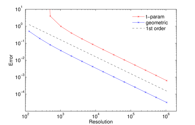
Fig. 1: Convergence of $x(t=0)$ to the analytical solution for the first test problem. Due to the choice of the time integration scheme, both methods converge to the analytical solution in first order. For a given resolution, the reparametrized method is more accurate by a factor $>10$.

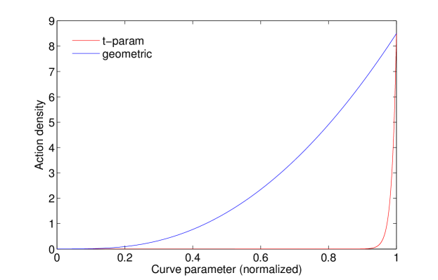
Fig. 2: Action density against curve parameter. For the simple iterative method, the curve parameter corresponds to the (normalized) physical time $t$. In the reparametrized method, regions with large action density are resolved better.

4.2 Application to the $\phi^{4}$ model

Consider the following SPDE

$$\phi_{t}=\phi_{xx}-\phi^{3}+\sqrt{2\epsilon}\,\eta(x,t),\qquad x\in(-L,L)$$ (37)

with Dirichlet boundary conditions $\phi(-L)=\phi(L)=0$, and where $\eta(x,t)$ is a spatio-temporal white-noise. It can be shown [8] that this equation is well-posed, and that its equilibrium distribution is formally given by

$$\mu(\phi)\propto\exp\left(-\epsilon^{-1}\int_{-L}^{L}(\tfrac{1}{2}|\phi_{x}|^{2}+\tfrac{1}{4}|\phi|^{4})dx\right).$$ (38)

The right way to interpret this measure is via its Radon-Nikodym derivative with respect to the measure of the Brownian bridge (i.e. by using the measure of the Brownian bridge as reference and writing the density of the equilibrium distribution of (37) with respect to this measure – see e.g. [18]):

$$\frac{d\mu}{d\nu}=\exp\left(-\tfrac{1}{4}\epsilon^{-1}\int_{-L}^{L}|B|^{4})dx\right),$$ (39)

where $\nu$ denotes the measure of the Brownian bridge $B(x)$ on $[-L,L]$, i.e. of the Gaussian process with mean zero and covariance

$$\mathbb{E}B(x)B(y)=\min(x+L,y+L)-\frac{(x+L)(y+L)}{2L}.$$ (40)

In the large deviation regime (i.e. in the limit when $\varepsilon\to 0$), we can ask what is the most likely configuration on the invariant measure such that $\phi(0)=\phi_{0}$. This is the solution of

$$\frac{d^{2}\phi}{dx^{2}}=\phi^{3},\quad\phi(0)=\phi_{0},\quad\phi(\pm L)=0$$ (41)

In the limit as $L\to\infty$, this solution is simply

$$\phi(x)=\frac{\phi_{0}}{1+\phi_{0}|x|/\sqrt{2}}.$$ (42)

We can also compute

$$\mathbb{E}\exp\left(\epsilon^{-1}\lambda\phi(0)\right),$$ (43)

where $\lambda>0$ is a parameter and the expectation is taken on the invariant measure. The configuration on the invariant measure that contributes the most to this expectation is the solution to (41) with the boundary condition $\phi_{x}(0+)=-\phi_{x}(0-)=-\lambda$ and $\phi(\pm L)=0$:

$$\phi(x)=\frac{\sqrt{\lambda}}{1+\sqrt{\lambda}|x|/\sqrt{2}}.$$ (44)

The path of maximum likelihood to get dynamically to (42) or (44) is then the time reversed of the solution to (37) with $\varepsilon=0$ (deterministic flow), and (42) or (44) as initial condition.

A similar story holds if we consider (37) with periodic boundary conditions, which are easier to implement numerically. In this case the solution to (41) with the boundary condition $\phi_{x}(0+)=-\phi_{x}(0-)=-\lambda$ and $\phi(L)=\phi(-L)$ gives the relevant configuration for the periodic case.

In this example, we implemented the iterative scheme, both for the equations of motion in the time-parametrized and the geometric variant by using a second order Heun integration in the curve parameter. The $x$-dimension is resolved with $N_{x}=512$ grid-points, using Fourier transforms to calculate the spatial derivatives.

Figure 3 compares, for different resolutions, the numerical solutions of the final configuration of the minimizer to the model (37) to the analytic solution for the periodic case. At a resolution of $N_{t}=512$, the geometric method already outperforms the time-parametrized variant with a considerably higher resolution of $N_{t}=16384$ in terms of accuracy.

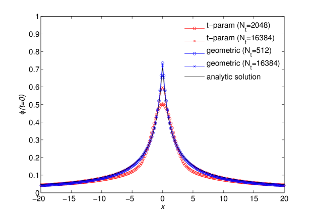
Fig. 3: Zoom to the origin for the final configuration in the proposed method and the time-parametrized method, in comparison to the analytical solution for the model system (37). The geometric solution at a moderate resolution of $N_{t}=512$ approximates the analytical solution better than the time-parametrized solution at a higher resolution of $N_{t}=16384$.

4.3 Application to the stochastically driven Burgers equation

Consider the stochastically driven Burger’s equation with periodic boundary conditions:

$$u_{t}=B(u)+\xi(x,t),\qquad B(u)=-uu_{x}+\nu u_{xx}.$$ (45)

In this example, we consider a noise term $\xi$ that has a finite correlation length in space, but is still $\delta$-correlated in time. Hence we can write

$$\langle\xi(x,t)\xi(x^{\prime},t^{\prime})\rangle=\chi(x-x^{\prime})\delta(t-t^{\prime})$$ (46)

and for the correlation function in space, we assume the following form in Fourier space

$$\hat{\chi}(\omega)=\omega^{2}\,{\mathrm{e}}^{-\omega^{2}/2}{\mathcal{H}}(\omega_{c}-|\omega|),$$ (47)

where ${\mathcal{H}}$ denotes the Heaviside-function. This form implies that the stochastic driving occurs only at frequencies up to a cut-off frequency $\omega_{c}$. In this way, (45) is a simple model for turbulence [2]: The system is stochastically driven at larger scales by the noise term $\xi$. This energy is transported via the non-linearity $uu_{x}$ from large scales to small scales where energy is dissipated due to the presence of the diffusive term $\nu u_{xx}$.

We consider the velocity field starting at rest for $t\rightarrow-\infty$ and we are interested in noise realizations that lead to strong negative gradients at $t=0$. This setup is similar to the analytic treatment in [1]. We choose as our observable

$${\mathcal{O}}(u)=\int w(x)u_{x}(x)\,dx,\qquad w(x)=\frac{1}{\sqrt{2\pi\sigma^{2}}}{\mathrm{e}}^{-x^{2}/(2\sigma^{2})}.$$ (48)

For this case, our Hamiltonian equations for the reparametrized fields $u(x,s)$, $p(x,s)$ can be written as

$$\begin{cases}\displaystyle u_{s}=\frac{\|u_{s}\|_{\chi}}{\|B(u)\|_{\chi}}\left(\int\chi(x-x^{\prime})p(x^{\prime})dx^{\prime}+B(u)\right)\\[8.0pt] \displaystyle p_{s}=-\frac{\|u_{s}\|_{\chi}}{\|B(u)\|_{\chi}}\left(up_{x}+\nu p_{xx}\right).\end{cases}$$ (49)

The initial condition for the velocity field $u$ is $u(s=0)=0$ for the final condition for the auxiliary field $p$ is $p(s=1)=-w_{x}$ as can be seen from (48) using integration by parts. The norm $\|\cdot\|_{\chi}$ is given by the inverse of $\chi$ on its support (which is compact in Fourier domain), hence

$$\|f\|_{\chi}=\left(\left\langle f,{\mathcal{F}}^{-1}\left(\hat{\chi}^{-1}\hat{f}\right)\right\rangle\right)^{1/2},$$ (50)

where, ${\mathcal{F}}^{-1}$ denotes the inverse Fourier transform operator and $\hat{f}=\mathcal{F}f$ is the Fourier transform of $f$.

For comparison with previous work [3, 12], it is useful to contrast (49) with the corresponding instanton equations in the original parametrization (using the time $t$ as parameter)

$$\begin{cases}\displaystyle u_{t}+uu_{x}-\nu u_{xx}=\int\chi(x-x^{\prime})p(x^{\prime})dx^{\prime}\\ \displaystyle p_{t}+up_{x}+\nu p_{xx}=0.\end{cases}$$ (51)

Note that the same equations can also be obtained using the Martin-Siggia-Rose/Janssen/de Dominicis formalism [16, 15, 4, 17]. A main problem in solving (51) with the boundary conditions $u=0$ at $t\rightarrow-\infty$ and $p(0-,x)=-w_{x}$ consists in the fact that the fixpoint of the system is only reached in the limit $t\rightarrow-\infty$ and not in finite time. When Chernykh and Stepanov computed a numerical solution to the system above, they used a combination of two clever tricks to mitigate this difficulty: First, they used self-similar properties of the heat-kernel to design a coordinate transform that leads to an exponential rescaling in time, second they used the linearization of the system around zero in order to replace the boundary condition $u=0$ by $u=\chi_{0}p$ (where the constant $\chi_{0}$ can be computed from the correlation function $\chi$). In the following we show that the geometric reformulation of the instanton equations leads to a natural rescaling of time that allows for direct efficient numerical solution, which is furthermore transferable to similar situations without any modification.

We implemented the iterative algorithm outlined in section 3, employing a second order Heun integration of the geometric equations of motion (49) and compare the results to a similar iterative algorithm, but integrating the time-parametrized equations of motion (51), instead. The space variable is resolved with $N_{x}=512$ grid-points, and all derivatives in space are calculated via Fourier transforms. For the calculations presented here we took $\sigma=0.1$ and $\nu=1/2$ in (48)

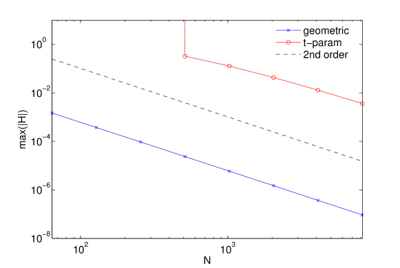
Fig. 4: Convergence of the maximum of the Hamiltonian along the minimizer. Both methods converge second order. For the smallest tested resolution of $N_{t}=64$ the error of the geometric integration still is smaller than the error of the time-parametrized integration at the highest tested resolution of $N_{t}=8192$ (overall $\approx 10^{4}$ times more accurate).

Figure 4 shows the convergence of the maximum of the Hamiltonian for the proposed scheme in comparison to the time-parametrized variant. For both methods the Hamiltonian converges to $0$ in second order. The reparametrized variant is a factor $>10^{4}$ more accurate: For the smallest tested resolution of $N_{t}=64$ the error of the geometric integration is still smaller than the error of the time-parametrized integration at the highest tested resolution of $N_{t}=8192$. The reason is simple:

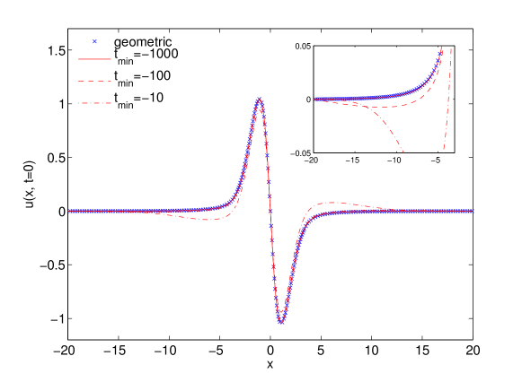
Fig. 5: Final configurations of the minimizer for different choices of the starting-time $t_{\text{min}}$ in comparison to the geometric variant. A choice of $t_{\text{min}}=-10$ and, to a much lesser extend, $t_{\text{min}}=-100$ produce secondary extrema (compare the zoom in the inset), which are absent for both $t_{\text{min}}=-1000$ and the geometric version.

When using physical time as discretization, it is necessary to prescribe a finite starting-time $t_{\text{min}}$ which is restricted in its magnitude to ensure stability and accuracy of the integration scheme for a given time resolution. Yet, when choosing $t_{\text{min}}$ too close to $0$, the resulting finite-time minimizer does not necessarily approximate the global minimizer. For the geometric equations of motion this issue is absent, and the arbitrary choice of $t_{\text{min}}$ is avoided in a natural way. Figure 5 depicts the final configurations of the minimizer for different choices of $t_{\text{min}}$, demonstrating the necessity to choose a sufficiently small starting time: A choice of $t_{\text{min}}=-10$ and, to a much lesser extend, $t_{\text{min}}=-100$ produce secondary extrema, which are absent for both $t_{\text{min}}=-1000$ and the geometric version.

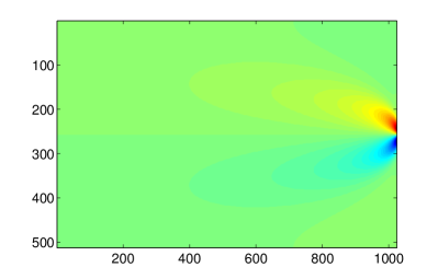
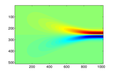
Fig. 6: Comparison of the minimizing field configuration for the time-parametrized equations of motion with $t_{\text{min}}=-100$ (left) and the geometric equations of motion (right) in space and time. Most of the dynamics happen in a small interval near $t=0$, which is well resolved in the geometric case.

A plot of the complete minimizer in space-time, as shown in figure 6, reveals the superior parametrization of the geometric scheme. Even for a somewhat optimistic choice of $t_{\text{min}}=-100$, most of the dynamics are squeezed into very few grid-points for the time-parametrization (left), while being far better resolved in the geometric case (right), which nevertheless covers a more than 10 times larger interval of physical time in total.

5 Conclusion

We presented a new method to compute minimizers of action functionals using a geometric reparametrization of Hamilton’s equations. The new method is particularly well-suited to compute expectations related to stochastically driven exits from attracting domains, though it may be useful in other contexts as well. The new method was illustrated using a simple Ornstein-Uhlenbeck system and then numerically implemented and tested in the context of stochastic partial differential equations with additive noise for the $\phi^{4}$-model and the stochastic Burgers equation. In all cases, it was shown that the new parametrization has computational advantages over the parametrization using the original physical time. Applications to more complicated systems, in particular higher-dimensional stochastic partial differential equations (e.g. stochastically driven Navier-Stokes or MHD equations) are therefore within reach and will be the topic of future research.

References

- [1] E. Balkovsky, G. Falkovich, I. Kolokolov, and V. Lebedev. Intermittency of Burgers’ turbulence. Phys. Rev. Lett., 78:1452, 1997.
- [2] J. Cardy, G. Falkovich, and K. Gawedzki. Non-equilibrium Statistical Mechanics and Turbulence. Cambridge University Press, 2008.
- [3] A.I. Chernykh and M.G. Stepanov. Large negative velocity gradients in Burgers turbulence. Phys. Rev. E, 64:026306, 2001.
- [4] C. de Dominicis. Techniques de renormalisation de la théorie des champs et dynamique des phénomènes critiques. J. Phys. C, 1:247, 1976.
- [5] W. E, W. Ren, and E. Vanden-Eijnden. String method for the study of rare events. Phys. Rev. B, 66:052301, 2002.
- [6] W. E, W. Ren, and E. Vanden-Eijnden. Minimum action method for the study of rare events. Comm. Pure Appl. Math., 57:1–20, 2004.
- [7] W. E, W. Ren, and E. Vanden-Eijnden. Simplified and improved string method for computing the minimum energy paths in barrier-crossing events. J. Chem. Phys., 126:164103, 2007.
- [8] W. G. Faris and G. Jona-Lasinio. Large fluctuations for a nonlinear heat equation with noise. J. of Phys. A, 15(10):3025, 1982.
- [9] H. C. Fogedby and W. Ren. Minimum action method for the Kardar-Parisi-Zhang equation. Phys. Rev. E, 80:041116, 2009.
- [10] M. I. Freidlin and A. D. Wentzell. Random perturbations of dynamical systems. Springer, 1998.
- [11] C. Gardiner. Stochastic Methods: A Handbook for the Natural and Social Sciences. Springer, 2009.
- [12] T. Grafke, R. Grauer, and T. Schäfer. Instanton filtering for the stochastic Burgers equation. J. Phys. A: Mathematical and Theoretical, 46(6):62002, 2013.
- [13] M. Heymann and E. Vanden-Eijnden. The geometric minimum action method: A least action principle on the space of curves. Comm. Pure and Appl. Math., 61:1053, 2008.
- [14] M. Heymann and E. Vanden-Eijnden. Pathways of maximum likelihood for rare events in nonequilibrium systems: application to nucleation in the presence of shear. Phys. Rev. Lett., 100(14):140601, 2008.
- [15] H. K. Janssen. On a Lagrangian for classical field dynamics and renormalization group calculations of dynamical critical properties. Z. Physik B, 23:377, 1976.
- [16] P. C. Martin, E. D. Siggia, and H. A. Rose. Statistical dynamics of classical systems. Phys. Rev. A, 8:423, 1973.
- [17] R. Phythian. The functional formalism of classical statistical dynamics. J. Phys. A, 10, 1977.
- [18] M. G. Reznikoff and E. Vanden-Eijnden. Invariant measures of stochastic partial differential equations and conditioned diffusions. Comptes Rendus Mathematique, 340(4):305–308, 2005.
- [19] E. Vanden-Eijnden and M. Heymann. The geometric minimum action method for computing minimum energy paths. J. Chem. Phys., 128:061103, 2008.
- [20] S. R. S. Varadhan. Large deviations. Ann. Prob., 36(2):397–419, 2008.
- [21] X. Zhou, W. Ren, and W. E. Adaptive minimum action method for the study of rare events. J. Chem. Phys., 128:104111, 2008.