System-size independence of a large deviation function for frequency of events in a one-dimensional forest-fire model with a single ignition site

Abstract

It is found that a large deviation function for frequency of events of size not equal to the system size in the one dimensional forest-fire model with a single ignition site at an edge is independent of the system size, by using an exact decomposition of the modified transition matrix of a master equation. An exchange in the largest eigenvalue of the modified transition matrix may not occur in the model.

1 Introduction

Non-equilibrium phenomena are omnipresent. Sometimes a rare phenomenon can cause massive effect on our everyday life. Recently a study on a large deviation function (LDF), which includes all the higher fluctuations, was extensively conducted in the context of non-equilibrium statistical physics [1, 2, 3, 4, 5]. The LDF describes the probability of rare events, and disastrous events such as large earthquakes can be characterized by the LDF. Moreover, phase transition between active and inactive phase is characterized by the LDF for an activity in a model of glassy dynamics [6]. The approach using the LDF to dynamic behaviours is soundly progressing [6, 7, 8, 9], however, studies concerning the LDF and criticality are yet developing.

In this study, we apply an approach using the LDF to the dynamic behaviours of a forest-fire model. Originally, Bak et alintroduced the forest-fire model to simulate the system with temporally uniform injection and fractal dissipation of energy [10]. The forest-fire model introduced by Bak et alis later extended by Drossel and Schwabl [11] in the context of self organaized criticality (SOC). Drossel and Schwabl represented forest-fire in the model with four processes: planting of trees, ignition, propagation of fire, and extinguishing of fire. To separate the timescale of the planting process and those of the latter three, an effective forest-fire model was introduced to analyze the model [12, 13]. The effective model reduces the last three processes to a single process, the vanishing of a cluster of trees. Moreover, the effective forest-fire model can be formalized by a master equation [14] and an analytical methods can be applied.

The forest-fire model is also considered as a model of earthquakes [15]. As an earthquake model, the planting of a tree corresponds to the loading of stress on the fault and the vanishing of a cluster of trees corresponds to the triggering of an earthquake which releases the stress on the connected loaded sites. A model similar to the one-dimensional forest-fire model with single triggering site at an edge was introduced as the minimalist model of earthquakes [16]. The distributions of trigger sites change the size-frequency distributions of earthquakes in two-dimensional forest-fire models [17]. Recently, the LDFs for frequency of the largest earthquake in forest-fire models with different distributions of trigger sites was numerically calculated, and a nearly periodic to Poisson occurrence depending on parameters and distribution of trigger sites is found [18].

Here, we focus on the model M1, which is the one-dimensional forest-fire model with single ignition site at an edge [18]. M1 is expressed by a master equation, and a standard method to calculate the LDF with a modified transition matrix of the master equation [19] can be applied to obtain the LDF for frequency of events. The LDF is given by the Legendre transform of a generating function which is equal to the largest eigenvalue of the modified transition matrix. In this study, we derived an exact decomposition of the modified transition matrix for the frequency of events of size smaller than the system size in M1, by applying a similarity transformation. The decomposition implies the system size independence of the LDF for the frequency. We numerically calculated the LDF for any system size and compared to that of the homogeneous Poisson process. The decomposition enables us to discuss the exchange of the largest and the second largest eigenvalue of the modified transition matrix in the limit of infinitely large system size.

We give introduction for the model we use in this study, the LDF and the method to calculate the LDF. Next we derive the decomposition of the modified transition matrix. Then, we give numerical calculations of the LDF. In the end, we present discussions.

2 Model and Method

2.1 Model

A forest-fire model with single ignition site at an edge is called M1 (figure 1). M1 can be written by a master equation as,

$$\frac{{\rm d}P(C;t)}{{\rm d}t}=\sum_{C^{\prime}}W_{L}(CC^{\prime})P(C^{\prime};t),$$ (1)

where $C$ denotes the configuration of the system, $P(C;t)$ is the probability of the system in $C$ at time $t$ and $W_{L}(CC^{\prime})$ is the transition probability rate from $C^{\prime}$ to $C$ with system size $L$. M1 consists of two processes: a loading process and a triggering process. The loading process represents the loading of stress onto a fault and the triggering process represents the occurence of an earthquake. $W_{L}(CC^{\prime})$ is denoted $p$ if the transition from $C^{\prime}$ to $C$ is the loading process and is denoted $f$ if the transition is the triggering process. We introduce $\tau_{j}\in\{0,1\}$ which represents the state of the site $j$ with $1\leq j\leq L$. $\tau_{j}=1$ represents loaded state and $\tau_{j}=0$ represents unloaded state. The configuration $C$ can be written as $C=\{\tau_{1},\cdots,\tau_{L}\}$. For example, the system is in the state $C=\{1,1,0,1,0\}$ as in figure 1. The loading process at the site in the middle is expressed by a transition from $\{1,1,0,1,0\}$ to $\{1,1,1,1,0\}$. The triggering process is expressed by a transition from $\{1,1,0,1,0\}$ to $\{0,0,0,1,0\}$ and the size of the event is $2$. A transition from $\{1,1,0,1,0\}$ to $\{1,1,0,0,0\}$ is not allowed in this model because the triggering only occur from the site $1$. The transition rates for $C\neq C^{\prime}$ can be written by $\tau_{j}$ as,

$$W_{L}(CC^{\prime})=p\sum_{j=1}^{L}[\cdots\delta_{\tau_{j-1}\tau^{\prime}_{j-1}}(1-\tau^{\prime}_{j})\tau_{j}\delta_{\tau_{j+1}\tau^{\prime}_{j+1}}\cdots]$$

$$+f\sum_{j=1}^{L}[\tau^{\prime}_{1}(1-\tau_{1})\cdots\tau^{\prime}_{j}(1-\tau_{j})(1-\tau^{\prime}_{j+1})(1-\tau_{j+1})\delta_{\tau_{j+2}\tau^{\prime}_{j+2}}\cdots],$$ (2)

where $\delta_{xx^{\prime}}$ is the Kronecker delta. The parts with a suffix less than $1$ or greater than $L$ are omitted. $W_{L}(CC^{\prime})$ for $C=C^{\prime}$ is written as,

$$W_{L}(CC^{\prime})=-p\sum_{j=1}^{L}[\cdots\delta_{\tau_{j-1}\tau^{\prime}_{j-1}}(1-\tau^{\prime}_{j})(1-\tau_{j})\delta_{\tau_{j+1}\tau^{\prime}_{j+1}}\cdots]$$

$$-f\sum_{j=1}^{L}[\tau^{\prime}_{1}\tau_{1}\cdots\tau^{\prime}_{j}\tau_{j}(1-\tau^{\prime}_{j+1})(1-\tau_{j+1})\delta_{\tau_{j+2}\tau^{\prime}_{j+2}}\cdots].$$ (3)

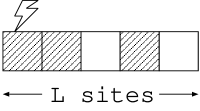
Figure 1: A schematic picture of the model M1. Shaded sites represent loaded sites, blank sites represent unloaded sites and a thunder mark represents an trigger site. If an event is triggered in this configuration, the two loaded sites in the left become empty, and the size of the event is $2$.

The master equation is transformed into a matrix representation as,

$$\frac{{\rm d}}{{\rm d}t}{\bf P}(t)=\mathsf{W}_{L}{\bf P}(t),$$ (4)

where ${\bf P}^{t}(t)=(P_{1}(t),\cdots,P_{2^{L}}(t))$, the index $\mu$ of $P_{\mu}(t)$ is given by $\mu=\sum_{i=1}^{L}\tau_{i}2^{i-1}$, and $\mathsf{W}_{L}$ is a transition matrix for the system size $L$. The index $\mu$ has one to one correspondence with the configuration $C$. For $L=2$, the explicit form of transition matrix is written as,

$$\mathsf{W}_{2}=\left(\begin{array}[]{cccc}-2p&f&0&f\\ p&-p-f&0&0\\ p&0&-p&0\\ 0&p&p&-f\end{array}\right),$$ (5)

and for $L=3$,

$$\mathsf{W}_{3}=\left(\begin{array}[]{cccccccc}-3p&f&0&f&0&0&0&f\\ p&-2p-f&0&0&0&0&0&0\\ p&0&-2p&0&0&0&0&0\\ 0&p&p&-p-f&0&0&0&0\\ p&0&0&0&-2p&f&0&0\\ 0&p&0&0&p&-p-f&0&0\\ 0&0&p&0&p&0&-p&0\\ 0&0&0&p&0&p&p&-f\end{array}\right).$$ (6)

2.2 Large deviation function

The mean frequency of events of size $s$ per unit time $x(s)$ is written as

$$x(s)=\frac{N(s)}{t}.$$ (7)

Here, $N(s)$ is the number of events of size $s$ for elapsed time $t$. The probability of $x(s)$, $P(x(s))$, asymptotically behaves as

$$P(x(s))\sim\exp[-t\phi(x(s))]$$ (8)

for large $t$, where the function $\phi(x(s))$ is called a large deviation function (LDF) for the frequency of events of size $s$. The LDF satisfies $\phi(x_{\rm m}(s))=0$ where $x_{\rm m}(s)$ is the frequency giving the minimum of $\phi(x(s))$. A large deviation function $\phi(x(s))$ has a corresponding ‘generating function’ $\mu_{s}(\lambda)$, where $\lambda$ is the conjugate variable of $x(s)$. The generating function $\mu_{s}(\lambda)$ is defined as

$$\exp[\mu_{s}(\lambda)t]=\langle\exp[\lambda x(s)t]\rangle\sim\int\exp[(\lambda x^{\prime}-\phi(x^{\prime}))t]\rmd x^{\prime}.$$ (9)

$\phi(x(s))$ and $\mu_{s}(\lambda)$ are related by the Legendre transform as

$$\phi(x(s))=\max_{\lambda}[x(s)\lambda-\mu_{s}(\lambda)].$$ (10)

The LDF for the frequency of events in a homogeneous Poisson process is

$$\phi_{\rm P}(x)=x\log(\frac{x}{\alpha})-x+\alpha,$$ (11)

where $\alpha$ is the rate of event occurrence and the suffix ${\rm P}$ represents the Poisson process.

To calculate the LDF, the largest eigenvalue of a modified transition matrix $\mathsf{W}_{L}^{\lambda,s}$ is necessary, where $\lambda$ is a field related to the number of events of size $s$. The largest eigenvalue of the modified transition matrix is equal to the generating function [19]. By using (10), the LDF is obtained from $\mu_{s}(\lambda)$. The modified transition matrix is defined as $W^{\lambda,s}_{L}(CC^{\prime})=\exp[\lambda X(s;CC^{\prime})]W_{L}(CC^{\prime})$, where $X(s;CC^{\prime})$ is $1$ for the event of size $s$ and $X(s;CC^{\prime})=0$ otherwise. The off-diagonal part of the modified transition rates is written as,

$$W_{L}^{\lambda,s}(CC^{\prime})=p\sum_{j=1}^{L}[\cdots\delta_{\tau_{j-1}\tau^{\prime}_{j-1}}(1-\tau^{\prime}_{j})\tau_{j}\delta_{\tau_{j+1}\tau^{\prime}_{j+1}}\cdots]$$

$$+f\sum_{j=1}^{L}[\exp(\lambda\delta_{j,s})\tau^{\prime}_{1}(1-\tau_{1})\cdots\tau^{\prime}_{j}(1-\tau_{j})(1-\tau^{\prime}_{j+1})(1-\tau_{j+1})\delta_{\tau_{j+2}\tau^{\prime}_{j+2}}\cdots].$$ (12)

The modified transition matrix for $L=2$ with $s=1$ is written as,

$$\mathsf{W}_{2}^{\lambda,1}=\left(\begin{array}[]{cccc}-2p&f\rme^{\lambda}&0&f\\ p&-p-f&0&0\\ p&0&-p&0\\ 0&p&p&-f\end{array}\right),$$ (13)

and for $L=3$,

$$\mathsf{W}_{3}^{\lambda,1}=\left(\begin{array}[]{cccccccc}-3p&f\rme^{\lambda}&0&f&0&0&0&f\\ p&-2p-f&0&0&0&0&0&0\\ p&0&-2p&0&0&0&0&0\\ 0&p&p&-p-f&0&0&0&0\\ p&0&0&0&-2p&f\rme^{\lambda}&0&0\\ 0&p&0&0&p&-p-f&0&0\\ 0&0&p&0&p&0&-p&0\\ 0&0&0&p&0&p&p&-f\end{array}\right).$$ (14)

3 System size independence of the LDF

By observing the forms of $\mathsf{W}_{2}^{\lambda,1}$ (13) and $\mathsf{W}_{3}^{\lambda,1}$ (14), we find that these two matrices are related as,

$$\mathsf{W}_{3}^{\lambda,1}=\left(\begin{array}[]{cc}\mathsf{W}_{2}^{\lambda,1}-pI_{2}&X_{2}\\ pI_{2}&\mathsf{W}_{2}^{\lambda,1}-X_{2}\end{array}\right),$$ (15)

where $I_{2}$ is the identity matrix of size $2^{2}\times 2^{2}$ and $X_{2}$ is defined as,

$$X_{2}=\left(\begin{array}[]{cccc}0&0&0&f\\ 0&0&0&0\\ 0&0&0&0\\ 0&0&0&0\end{array}\right).$$ (16)

By applying a similarity transformation, $\mathsf{W}_{3}^{\lambda,1}$ satisfies

$$\mathsf{W}^{\lambda,1}_{3}\sim\left(\begin{array}[]{cc}\mathsf{W}_{2}^{\lambda,1}-pI_{2}-X_{2}&-pI_{2}+X_{2}\\ 0&\mathsf{W}_{2}^{\lambda,1}\end{array}\right).$$ (17)

Thus, the eigenvalues of $\mathsf{W}_{3}^{\lambda,1}$ are composed of the eigenvalues of $\mathsf{W}_{2}^{\lambda,1}$ and $\mathsf{W}_{2}^{\lambda,1}-pI_{2}-X_{2}$.

Next we derive the relation between $\mathsf{W}^{\lambda,s}_{L+1}$ and $\mathsf{W}^{\lambda,s}_{L}$. The $\mathsf{W}^{\lambda,s}_{L+1}$ is written as,

$$W_{L+1}^{\lambda,s}(CC^{\prime})=p\sum_{j=1}^{L+1}[\cdots\delta_{\tau_{j-1}\tau^{\prime}_{j-1}}(1-\tau^{\prime}_{j})\tau_{j}\delta_{\tau_{j+1}\tau^{\prime}_{j+1}}\cdots]$$

$$+f\sum_{j=1}^{L+1}[\exp(\lambda\delta_{j,s})\tau^{\prime}_{1}(1-\tau_{1})\cdots\tau^{\prime}_{j}(1-\tau_{j})(1-\tau^{\prime}_{j+1})(1-\tau_{j+1})\delta_{\tau_{j+2}\tau^{\prime}_{j+2}}\cdots]$$

$$-p\sum_{j=1}^{L+1}[\cdots\delta_{\tau_{j-1}\tau^{\prime}_{j-1}}(1-\tau^{\prime}_{j})(1-\tau_{j})\delta_{\tau_{j+1}\tau^{\prime}_{j+1}}\cdots]$$

$$-f\sum_{j=1}^{L+1}[\tau^{\prime}_{1}\tau_{1}\cdots\tau^{\prime}_{j}\tau_{j}(1-\tau^{\prime}_{j+1})(1-\tau_{j+1})\delta_{\tau_{j+2}\tau^{\prime}_{j+2}}\cdots].$$ (18)

$\mathsf{W}^{\lambda,s}_{L+1}$ is written by using $\mathsf{W}^{\lambda,s}_{L}$ as,

$$\mathsf{W}^{\lambda,s}_{L+1} = \mathsf{W}^{\lambda,s}_{L}\delta_{\tau_{L+1}\tau^{\prime}_{L+1}}+p\delta_{\tau_{1}\tau^{\prime}_{1}}\cdots\delta_{\tau_{L}\tau^{\prime}_{L}}(1-\tau^{\prime}_{L+1})\tau_{L+1}$$ (19)

$$-p\delta_{\tau_{1}\tau^{\prime}_{1}}\cdots\delta_{\tau_{L}\tau^{\prime}_{L}}(1-\tau^{\prime}_{L+1})(1-\tau_{L+1})$$

$$+f\tau^{\prime}_{1}(1-\tau_{1})\cdots\tau^{\prime}_{L}(1-\tau_{L})\tau^{\prime}_{L+1}(1-\tau_{j+1})$$

$$-f\tau^{\prime}_{1}(1-\tau_{1})\cdots\tau^{\prime}_{L}(1-\tau_{L})\tau_{L+1}\tau^{\prime}_{L+1}$$

(19) is also written in the matrix form as,

$$\mathsf{W}^{\lambda,s}_{L+1}=\left(\begin{array}[]{cc}\mathsf{W}^{\lambda,s}_{L}-p\delta_{\tau_{1}\tau^{\prime}_{1}}\cdots\delta_{\tau_{L}\tau^{\prime}_{L}}&f\tau^{\prime}_{1}(1-\tau_{1})\cdots\tau^{\prime}_{L}(1-\tau_{L})\\ p\delta_{\tau_{1}\tau^{\prime}_{1}}\cdots\delta_{\tau_{L}\tau^{\prime}_{L}}&\mathsf{W}^{\lambda,s}_{L}-f\tau^{\prime}_{1}(1-\tau_{1})\cdots\tau^{\prime}_{L}(1-\tau_{L})\end{array}\right)$$ (22)

$$= \left(\begin{array}[]{cc}\mathsf{W}^{\lambda,s}_{L}-pI_{L}&X_{L}\\ pI_{L}&\mathsf{W}^{\lambda,s}_{L}-X_{L}\end{array}\right).$$ (25)

where $I_{L}=\prod_{i=1}^{L}\delta_{\tau_{i}\tau^{\prime}_{i}}$ and

$$X_{L}=\left(\begin{array}[]{ccc}0&\cdots&f\\ \vdots&\ddots&\vdots\\ 0&\cdots&0\end{array}\right).$$ (26)

$X_{L}$ corresponds to the term $f\tau^{\prime}_{1}(1-\tau_{1})\cdots\tau^{\prime}_{L}(1-\tau_{L})$. A similarity transformation leads to

$$\mathsf{W}^{\lambda,s}_{L+1}\sim\left(\begin{array}[]{cc}\mathsf{W}_{L}^{\lambda,s}-pI_{L}-X_{L}&-pI_{L}+X_{L}\\ 0&\mathsf{W}_{L}^{\lambda,s}\end{array}\right).$$ (27)

Thus, the eigenvalues of $\mathsf{W}_{L+1}^{\lambda,s}$ are composed of the eigenvalues of $\mathsf{W}_{L}^{\lambda,s}$ and $\mathsf{W}_{L}^{\lambda,s}-pI_{L}-X_{L}$.

From (25), $\mathsf{W}_{L}^{\lambda,s}-pI_{L}-X_{L}$ is written as,

$$\mathsf{W}_{L}^{\lambda,s}-pI_{L}-X_{L}=\left(\begin{array}[]{cc}\mathsf{W}_{L-1}^{\lambda,s}-2pI_{L-1}&0\\ pI_{L-1}&\mathsf{W}_{L-1}^{\lambda,s}-pI_{L-1}-X_{L-1}\end{array}\right).$$ (28)

By using (27) and (28), $\mathsf{W}_{L}^{\lambda,s}$ is decomposed into $\mathsf{W}_{s+1}^{\lambda,s}-kpI_{s+1}$ for even $k$ and $\mathsf{W}_{s+1}^{\lambda,s}-kpI_{s+1}-X_{s+1}$ for odd $k$ with $k=\{0,\cdots,L-s-1\}$, where each component is degenerate ${}_{L-s-1}C_{k}$ times. Here we mean by decomposition that a set of eigenvalues of a matrix is decomposed into sets of eigenvalues of the component matrices. For example, from (17), $\mathsf{W}_{3}^{\lambda,1}$ is decomposed into $\mathsf{W}_{2}^{\lambda,1}$ and $\mathsf{W}_{2}^{\lambda,1}-pI_{2}-X_{2}$. The proof of the decomposition of $\mathsf{W}_{L}^{\lambda,s}$ is given in the appendix.

The decomposition of $\mathsf{W}_{L}^{\lambda,s}$ suggests that the largest eigenvalue of $\mathsf{W}_{L}^{\lambda,s}$ is included in the eigenvalues of $\mathsf{W}_{s+1}^{\lambda,s}$ or $\mathsf{W}_{s+1}^{\lambda,s}-pI_{s+1}-X_{s+1}$ for any $L>s$. The largest eigenvalues of the other components are smaller than the two components, because the term $-pkI_{L}$ just shifts all the eigenvalues. Among the decomposed elements, the eigenvalues of $\mathsf{W}_{2}^{\lambda,1}-pI_{2}-X_{2}$, which denote $\zeta_{1},\cdots,\zeta_{4}$, are calculated as,

$$\zeta_{1} = -2p$$ (29)

$$\zeta_{2} = -p-f$$ (30)

$$\zeta_{3} = \frac{-5p-f+\sqrt{(p-f)^{2}+4pf\rme^{\lambda}}}{2}$$ (31)

$$\zeta_{4} = \frac{-5p-f-\sqrt{(p-f)^{2}+4pf\rme^{\lambda}}}{2}.$$ (32)

However, the analytical forms of the eigenvalues of other cases are complex. For small $s$ and $L$, we can numerically calculate the largest eigenvalue of $\mathsf{W}_{s+1}^{\lambda,s}$ or $\mathsf{W}_{s+1}^{\lambda,s}-pI_{s+1}-X_{s+1}$.

The numerical calculations suggest that the largest eigenvalue of $\mathsf{W}_{2}^{\lambda,1}$ is larger than that of $\mathsf{W}_{2}^{\lambda,1}-pI_{2}-X_{2}$ (figure 2), for $0.01\leq f\leq 1$ and $-3\leq\lambda\leq 5$. Thus, the largest eigenvalue of $\mathsf{W}_{2}^{\lambda,1}$ is the largest eigenvalue of $\mathsf{W}_{L}^{\lambda,1}$. We assume that this holds for other $f$ and $\lambda$.

Figure 2: The difference between the largest eigenvalue of $\mathsf{W}_{2}^{\lambda,1}$ and that of $\mathsf{W}_{2}^{\lambda,1}-pI_{2}-X_{2}$ for $0.01\leq f\leq 1$ and $-3\leq\lambda\leq 5$. The difference is higher than $1$ for this parameter region which suggest the largest eigenvalue of $\mathsf{W}_{2}^{\lambda,1}$ is larger than that of $\mathsf{W}_{2}^{\lambda,1}-pI_{2}-X_{2}$.

The generating function corresponding to the LDF for frequency of events of size $s$ is equal to the largest eigenvalue of $\mathsf{W}^{\lambda,s}_{L}$. In figure 3(a), $\phi(z(1))/x_{\rm m}(1)$ for $L=2,6,10$ is plotted with $f=1.0,0.1$ and $0.01$. $z(s)$ is defined as $z(s)=(x(s)-x_{\rm m}(s))/x_{\rm m}(s)$. The numerically calculated LDFs are exactly the same as that of different $L$. The solid line denotes the LDF for frequency of a homogeneous Poisson process in $z$, $\phi_{\rm P}(z)=(z+1)\log(z+1)-z$. The LDFs for $f=0.1$ and $0.01$ are below $\phi_{\rm P}(z)$, which suggests that the fluctuation is larger than that of the Poisson process.

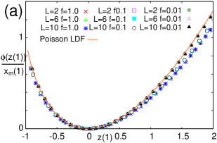
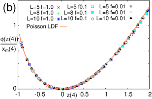
Figure 3: (a) $\phi(z(1))/x_{\rm m}(1)$ for $L=2,6,10$ and (b) $\phi(z(4))/x_{\rm m}(4)$ for $L=5,8,10$ with $f=1.0,0.1$ and $0.01$. The LDF takes the same value for different $L$.

In the figure 3(b), the LDF for frequency of $s=4$ is presented for $L=5,8,10$ and $f=1.0,0.1$ and $0.01$. The LDFs in the figure 3(b) is well approximated by the Poisson LDF.

4 Discussions

The decomposition of $\mathsf{W}_{L}^{\lambda,s}$ holds for any $L>s$. If we increase $L$ and continue the decomposition for many times, a newly produced component will have a lower shifted term, so that the eigenvalues are always smaller than that of $\mathsf{W}_{s+1}^{\lambda,s}$ or $\mathsf{W}_{s+1}^{\lambda,s}-pI_{s+1}-X_{s+1}$. Thus, the LDF or the largest eigenvalue of the modified transition matrix in the $L\to\infty$ limit is still the largest eigenvalue of $\mathsf{W}_{s+1}^{\lambda,s}$ or $\mathsf{W}_{s+1}^{\lambda,s}-pI_{s+1}-X_{s+1}$. For $s=1$, the claim that the largest eigenvalue is included in $\mathsf{W}_{2}^{\lambda,1}$ is supported by the numerical calculations. It is an open problem whether the largest eigenvalue is always included in $\mathsf{W}_{s+1}^{\lambda,s}$ or not. If the largest eigenvalue is exchanged with the other eigenvalues in the $L\to\infty$ limit, a dynamical phase transition may occur. A criticality for $L\to\infty$ is an important problem in the self organized criticality (SOC) point of view, since there has been intensive studies concerning the SOC of the forest-fire models based on simulations, for example see [20, 21]. Note that M1 is different from usual forest-fires in the distribution of trigger sites and in the absence of fire propagation process. It is an interesting development that if the approach based on the LDF in this study can contribute to such exciting problems. The decomposition found in this study is limited to M1, however the same structure might be found in other models written by master equations. The exchange of the largest eigenvalue and the second largest eigenvalue can be also discussed by numerical calculations of the models of interest, so that future development concerning the LDF and related phase transitions is largely expected.

We found an exact decomposition of the modified transition matrix concerning the frequency of events of size $s<L$ in the model M1. The decomposition leads to the independence of $L$ in the LDF for frequency of events of size $s<L$. However, for the events of size $L$, the LDF for frequency depend on $L$ [18]. Concerning earthquakes, relation between the LDF of frequency of small earthquakes and that of the system-size earthquakes is an interesting problem because the relation between them is related to the problem of capturing the symptoms of large earthquakes.

Appendix A Proof of the decomposition

We derived a similarity relation

$$\mathsf{W}^{\lambda,s}_{L}\sim\left(\begin{array}[]{cc}\mathsf{W}_{L-1}^{\lambda,s}-pI_{L-1}-X_{L-1}&-pI_{L-1}+X_{L-1}\\ 0&\mathsf{W}_{L-1}^{\lambda,s}\end{array}\right)$$ (33)

and an equation

$$\mathsf{W}_{L}^{\lambda,s}-pI_{L}-X_{L}=\left(\begin{array}[]{cc}\mathsf{W}_{L-1}^{\lambda,s}-2pI_{L-1}&0\\ pI_{L-1}&\mathsf{W}_{L-1}^{\lambda,s}-pI_{L-1}-X_{L-1}\end{array}\right)$$ (34)

for $\mathsf{W}_{L}^{\lambda,s}$. Using these two relations, we prove a proposition that ’$\mathsf{W}_{L}^{\lambda,s}$ is decomposed into $\mathsf{W}_{s+1}^{\lambda,s}-kpI_{s+1}$ for even $k$ and $\mathsf{W}_{s+1}^{\lambda,s}-kpI_{s+1}-X_{s+1}$ for odd $k$ which are degenerate ${}_{L-s-1}C_{k}$ times where $k=\{0,\cdots,L-s-1\}$’ by the mathematical induction.

For $L=s+2$, $\mathsf{W}^{\lambda,s}_{s+2}$ is decomposed into $\mathsf{W}^{\lambda,s}_{s+1}$ and $\mathsf{W}^{\lambda,s}_{s+1}-pI_{s+1}-X_{s+1}$. For $L=s+3$, $\mathsf{W}^{\lambda,s}_{s+3}$ is decomposed into $\mathsf{W}^{\lambda,s}_{s+1}$, two of $\mathsf{W}^{\lambda,s}_{s+1}-pI_{s+1}-X_{s+1}$ an $\mathsf{W}^{\lambda,s}_{s+1}-2pI_{s+1}$. For $L=s+4$, from (33) and (34),

$$\mathsf{W}_{s+4}^{\lambda,s}\sim\left(\begin{array}[]{cc}\mathsf{W}_{s+3}^{\lambda,s}-pI_{s+3}-X_{s+3}&-pI_{s+3}+X_{s+3}\\ 0&\mathsf{W}_{s+3}^{\lambda,s}\end{array}\right)$$ (35)

and

$$\mathsf{W}_{s+3}^{\lambda,s}-pI_{s+3}-X_{s+3}=\left(\begin{array}[]{cc}\mathsf{W}_{s+2}^{\lambda,s}-2pI_{s+2}&0\\ pI_{s+2}&\mathsf{W}_{s+2}^{\lambda,s}-pI_{s+2}-X_{s+2}\end{array}\right),$$ (36)

are satisfied. Thus, $\mathsf{W}_{s+4}^{\lambda,s}$ is decomposed into $\mathsf{W}_{s+3}^{\lambda,s},\mathsf{W}_{s+2}^{\lambda,s}-2pI_{s+2}$ and $\mathsf{W}_{s+2}^{\lambda,s}-pI_{s+2}-X_{s+2}$. $\mathsf{W}_{s+2}^{\lambda,s}-2pI_{s+2}$ is decomposed into $\mathsf{W}^{\lambda,s}_{s+1}-3pI_{s+1}-X_{s+1}$ and $\mathsf{W}^{\lambda,s}_{s+1}-2pI_{s+1}$. $\mathsf{W}_{s+2}^{\lambda,s}-pI_{s+2}-X_{s+2}$ is decomposed into $\mathsf{W}_{s+1}^{\lambda,s}-pI_{s+1}-X_{s+1}$ and $\mathsf{W}_{s+1}^{\lambda,s}-2pI_{s+1}$. By collecting all the components, $\mathsf{W}_{s+4}^{\lambda,s}$ is decomposed into $\mathsf{W}_{s+1}^{\lambda,s}$, $3$ of $\mathsf{W}_{s+1}^{\lambda,s}-pI_{s+1}-X_{s+1}$, $3$ of $\mathsf{W}_{s+1}^{\lambda,s}-2pI_{s+1}$ and $\mathsf{W}_{s+1}^{\lambda,s}-3pI_{s+1}-X_{s+1}$ (See table A1.). Thus, the proposition holds for $L=s+4$.

Table 1: Decomposition table for $L=3,\cdots,6$ and for odd $L$. $\mathsf{W}_{L}^{\lambda,s}$ is decomposed into the matrices in the left column, and the number of degeneracy is presented.

• 	$\mathsf{W}_{s+2}^{\lambda,s}$	$\mathsf{W}_{s+3}^{\lambda,s}$	$\mathsf{W}_{s+4}^{\lambda,s}$	$\mathsf{W}_{s+5}^{\lambda,s}$	$\cdots$	$\mathsf{W}_{L}^{\lambda,s}$
  $\mathsf{W}_{s+1}^{\lambda,s}$	1	1	1	1	$\cdots$	${}_{L-s-1}C_{0}$
  $\mathsf{W}_{s+1}^{\lambda,s}-pI_{s+1}-X_{s+1}$	1	2	3	4	$\cdots$	${}_{L-s-1}C_{1}$
  $\mathsf{W}_{s+1}^{\lambda,s}-2pI_{s+1}$	0	1	3	6	$\cdots$	${}_{L-s-1}C_{2}$
  $\mathsf{W}_{s+1}^{\lambda,s}-3pI_{s+1}-X_{s+1}$	0	0	1	4	$\cdots$	${}_{L-s-1}C_{3}$
  $\vdots$	$\vdots$	$\vdots$	$\vdots$	$\vdots$	$\ldots$	$\vdots$
  $\mathsf{W}_{s+1}^{\lambda,s}-(L-s-2)pI_{s+1}$	0	0	0	0	$\cdots$	${}_{L-s-1}C_{L-s-2}$
  $\mathsf{W}_{s+1}^{\lambda,s}-(L-s-2)pI_{s+1}-X_{s+1}$	0	0	0	0	$\cdots$	${}_{L-s-1}C_{L-s-1}$

Let us assume that $\mathsf{W}_{L}^{\lambda,s}$ is decomposed into $\mathsf{W}_{s+1}^{\lambda,s}-kpI_{s+1}$ for even $k$ and $\mathsf{W}_{s+1}^{\lambda,s}-kpI_{s+1}-X_{s+1}$ for odd $k$ which are degenerate ${}_{L-s-1}C_{k}$ times where $k=\{0,\cdots,L-s-1\}$, and also $\mathsf{W}_{L-1}^{\lambda,s}$ is decomposed into $\mathsf{W}_{s+1}^{\lambda,s}-kpI_{s+1}$ for even $k$ and $\mathsf{W}_{s+1}^{\lambda,s}-kpI_{s+1}-X_{s+1}$ for odd $k$ which are degenerate ${}_{L-s-2}C_{k}$ times where $k=\{0,\cdots,L-s-2\}$. $\mathsf{W}_{L+1}^{\lambda,s}$ is composed of $\mathsf{W}_{L}^{\lambda,s}-pI_{L}-X_{L}$ and $\mathsf{W}_{L}^{\lambda,s}$. $\mathsf{W}_{L}^{\lambda,s}-pI_{L}-X_{L}$ is composed of $\mathsf{W}_{L-1}^{\lambda,s}-pI_{L-1}-X_{L-1}$ and $\mathsf{W}_{L-1}^{\lambda,s}-2pI_{L-1}$. By subtracting the components of $\mathsf{W}_{L-1}^{\lambda,s}-2pI_{L-1}$ from the components of $\mathsf{W}_{L}^{\lambda,s}$, it directly follows that $\mathsf{W}^{\lambda,s}_{L-1}-pI_{L-1}-X_{L-1}$ is decomposed into $\mathsf{W}_{s+1}^{\lambda,s}-kpI_{s+1}$ for even $k$ and $\mathsf{W}_{s+1}^{\lambda,s}-kpI_{s+1}-X_{s+1}$ for odd $k$ which are degenerate ${}_{L-3}C_{k-1}$ times where $k=\{1,\cdots,L-s-1\}$. Also using the assumption, $\mathsf{W}_{L-1}^{\lambda,s}-2pI_{L-1}$ is decomposed into $\mathsf{W}_{s+1}^{\lambda,s}-(k+2)pI_{s+1}$ for even $k$ and $\mathsf{W}_{s+1}^{\lambda,s}-(k+2)pI_{s+1}-X_{s+1}$ for odd $k$ which are degenerate ${}_{L-3}C_{k-2}$ times where $k=\{2,\cdots,L-s\}$. The number of degeneracy and the decomposed elements are summarized in the table A2.

Table 2: The decomposition table for calculating $\mathsf{W}_{L+1}^{\lambda,s}$. The table is for odd $L$.

• component	$\mathsf{W}_{L}^{\lambda,s}$	$\mathsf{W}_{L-1}^{\lambda,s}-pI_{L-1}-X_{L-1}$	$\mathsf{W}_{L-1}^{\lambda,s}-2pI_{L-1}$	$\mathsf{W}_{L+1}^{\lambda,s}$
  $\mathsf{W}_{s+1}^{\lambda,s}$	${}_{L-s-1}C_{0}$	0	0	${}_{L-s}C_{0}$
  $\mathsf{W}_{s+1}^{\lambda,s}-pI_{s+1}-X_{s+1}$	${}_{L-s-1}C_{1}$	${}_{L-s-2}C_{0}$	0	${}_{L-s}C_{1}$
  $\mathsf{W}_{s+1}^{\lambda,s}-2pI_{s+1}$	${}_{L-s-1}C_{2}$	${}_{L-s-2}C_{1}$	${}_{L-s-2}C_{0}$	${}_{L-s}C_{2}$
  $\mathsf{W}_{s+1}^{\lambda,s}-3pI_{s+1}-X_{s+1}$	${}_{L-s-1}C_{3}$	${}_{L-s-2}C_{2}$	${}_{L-s-2}C_{1}$	${}_{L-s}C_{3}$
  $\vdots$	$\vdots$	$\vdots$	$\vdots$	$\vdots$
  $\mathsf{W}_{s+1}^{\lambda,s}-kpI_{s+1}$	${}_{L-s-1}C_{k}$	${}_{L-s-2}C_{k-1}$	${}_{L-s-2}C_{k-2}$	${}_{L-s}C_{k}$
  $\mathsf{W}_{s+1}^{\lambda,s}-(k+1)pI_{s+1}-X_{s+1}$	${}_{L-s-1}C_{k+1}$	${}_{L-s-2}C_{k}$	${}_{L-s-2}C_{k-1}$	${}_{L-s}C_{k+1}$
  $\vdots$	$\vdots$	$\vdots$	$\vdots$	$\vdots$
  $\mathsf{W}_{s+1}^{\lambda,s}-(L-s-2)pI_{s+1}$	${}_{L-s-1}C_{L-s-2}$	${}_{L-s-2}C_{L-s-3}$	${}_{L-s-2}C_{L-s-4}$	${}_{L-s}C_{L-s-2}$
  $\mathsf{W}_{s+1}^{\lambda,s}-(L-s-1)pI_{s+1}-X_{s+1}$	${}_{L-s-1}C_{L-s-1}$	${}_{L-s-2}C_{L-s-2}$	${}_{L-s-2}C_{L-s-3}$	${}_{L-s}C_{L-s-1}$
  $\mathsf{W}_{s+1}^{\lambda,s}-(L-s)pI_{s+1}$	$0$	$0$	${}_{L-s-2}C_{L-s-2}$	${}_{L-s}C_{L-s}$

As we see in the table A2, we can sum up the number of degeneracy of $\mathsf{W}_{s+1}^{\lambda,s}-kpI_{s+1}$ as ${}_{L-s-1}C_{k}+{}_{L-s-2}C_{k-1}+{}_{L-s-2}C_{k-2}$. The summation is equal to ${}_{L-s}C_{k}$ which is the same as the number of degeneracy for $\mathsf{W}_{L+1}^{\lambda,s}$. Thus, the decomposition of the $L+1$ matrix satisfy the proposition.

References

References

• [1] Derrida B and Lebowitz J L 1998 Phys. Rev. Lett. 80 209
• [2] Bertini L, De Sole A, Gabrielli D, Jona-Lasinio and Landim C 2001 Phys. Rev. Lett. 87 040601
• [3] Derrida B 2007 J. Stat. Mech. P07023
• [4] Touchette H 2009 Phys. Rep. 478 1
• [5] Giardinà C, Kurchan J, Lecomte V and Tailleur J 2011 J. Stat. Phys. 145 787
• [6] Garrahan J P, Jack R L, Lecomte V, Pitard E, van Duijvendijk K, and van Wijland F 2007 Phys. Rev. Lett. 98 195702
• [7] Rákos A and Harris R J 2008 J. Stat. Mech. P05005
• [8] de Gier J and Essler H L 2011 Phys. Rev. Lett. 107 010602
• [9] Cohen O and Mukamel D 2012 Phys. Rev. Lett. 108 060602
• [10] Bak P, Chen K and Tang C 1990 Phys. Lett. A 147 297
• [11] Drossel B and Schwabl F 1992 Phys. Rev. Lett. 69 1629
• [12] Henley C L 1993 Phys. Rev. Lett. 71 2741
• [13] Paczuski M and Bak P 1993 Phys. Rev. E 48 R3214
• [14] Honecker A and Peschel I 1996 Physica A 229 478
• [15] Turcotte D L, 1999 Rep. Prog. Phys. 62 1377; 1999 Phys. Earth. Planet. Inter. 111 275
• [16] Vázquez-Prada M, González Á, Gómez J B and Pacheco A F 2002 Nonlin. Proc. Geophys. 9 513
• [17] Tejedor A, Gómez J B and Pacheco A F 2009 Phys. Rev. E 79 046102
• [18] Mitsudo T and Kato N 2012 arXiv 1209.0879
• [19] Dembo A and Zeitouni O 1998 Large Deviations Techniques and Applications (Springer-Verlag, Berlin) p 71
• [20] Grassberger P 2002 New J. Phys. 4 17
• [21] Bonachela J A and Muñoz M A 2009 J. Stat. Mech: Theo. Exp. P09009