Separation of neutral and charge modes in one dimensional chiral edge channels
Abstract
Coulomb interactions have a major role in one-dimensional electronic transport. They modify the nature of the elementary excitations from Landau quasiparticles in higher dimensions to collective excitations in one dimension. Here we report the direct observation of the collective neutral and charge modes of the two chiral co-propagating edge channels of opposite spins of the quantum Hall effect at filling factor 2. Generating a charge density wave at frequency in the outer channel, we measure the current induced by inter-channel Coulomb interaction in the inner channel after a 3-mm propagation length. Varying the driving frequency from to GHz, we observe damped oscillations in the induced current that result from the phase shift between the fast charge and slow neutral eigenmodes. We measure the dispersion relation and dissipation of the neutral mode from which we deduce quantitative information on the interaction range and parameters.
Most studies of collective excitations in one dimensional systems performed so far have focused on non-chiral quantum wires Auslaender2005 ; Steinberg2007 ; Jompol2009 . In these systems, the collective excitations carrying the charge and the spin propagate at different velocities leading to the separation of the charge and spin degrees of freedom. This spin-charge separation has been probed by measuring the tunneling spectroscopy of individual electrons between a pair of one dimensional wires Auslaender2005 , or alternatively, between a wire and a two dimensional electron gas Jompol2009 . However, a direct observation of the collective modes is experimentally challenging as the relevant energy scales are too high for usual low frequency measurements.
The edge channels of the quantum Hall effect provide another implementation of one dimensional transport, where propagation is chiral and ballistic over large distances. These specificities have inspired several experiments that aim at reproducing, in solid state, optical setups where light beams are replaced by electron beamsHenny1999 ; Ji2003 ; Bocquillon2012 ; Bocquillon2013 . One major difference between electrons and photons comes from interaction effects, which are amplified in the one dimensional geometry and should enrich electron optics compared to its photonic counterpart. Of particular interest is the case of filling factor where transport along the sample edge occurs through two copropagating edge channels of opposite spins. Due to Coulomb interaction, the two edge states are coupled and new propagating eigenmodes, with different velocities, appearLee1997 ; Sukhorukov2007 ; Levkivskyi2008 ; Berg2009 ; Levkivskyi2012 , similarly to the physics arising in 1D wires. Consequently, considering edge channels with the same propagation characteristics (but different spins), and denoting the current components in edge channels and at position and time , a current in channel decomposes in the symmetric fast charge mode and the antisymmetric slow neutral mode (also called dipolar mode). As these two modes propagate at different velocities, the current initially injected in channel 1 separates into the charge and the neutral modes of the two coupled edges . This mechanism is at the heart of the decoherenceSukhorukov2007 ; Levkivskyi2008 ; Grenier2011 and relaxationKovrizhin2010 ; Degiovanni2010 ; Lunde2010 ; Levkivskyi2012 of electronic excitations propagating in these systems. As such, it has been probed through Mach-Zehnder interferometryNeder2006 ; Roulleau2008 ; Huynh or spectroscopy of edge channels Altimiras2009 ; Altimiras2010 ; LeSueur2010 . This situation bears strong analogies with the spin-charge separation of conventional 1D wires except that the two spin species are carried by two separated edge channels. The direct observation of the neutral and charge eigenmodes is thus particularly favorable in the filling factor 2 case as, contrary to a conventional wire, each spin channel can be individually addressed due to their spatial separation. Still, the observation remains challenging as transport properties remain unaffected up to GHz frequencies, where the wavelength of the eigenmodes becomes comparable with the propagation length of a few microns. Many experimental works have studied charge transport in quantum Hall edge channels and interaction effects between copropagating and counterpropagating edge channels either in time Ashoori1992 ; Zhitenev1993 ; Ernst1996 ; Sukhodub2004 or in frequency Gabellia ; Talyanskii1992 ; Hashisaka2012 ; Andreev2012 domains. However, none directly addressed the separation in charge and neutral modes as the individual control of edge channels was missing.
In this work, by addressing edge channels individually, we provide a direct observation of the neutral-charge eigenmodes. Using a driven mesoscopic capacitor (Fig.1 (a), see Methods for details), a sinusoidal charge density wave, or edge magnetoplasmon (EMP) is induced at pulsation and position in channel 1, thus creating a current (with ). As initially introduced in the context of a non chiral one dimensional wire Safi1995 and later developed for chiral edge channels Degiovanni2010 at filling factor , Coulomb interaction during propagation can be described as the scattering of the charge density waves. For the case of filling factor of interest here, scattering properties of EMPs are encoded in the scattering matrix that relates the amplitudes of the output EMP in channels 1 and 2 after propagation length to the amplitudes of the input EMP at . After an interaction length m, both edge channels reach a quantum point contact (QPC) which is used to transmit or reflect channels 1 and 2. Figure 1(b) presents the principle of measurement for two typical sets of data (for and 5.5 GHz). In configuration , channel 1 is transmitted and channel is reflected. The current in channel 2 resulting from the interaction, denoted , can then be measured in ohmic contact , with . When the QPC is closed (configuration 2), both channels are reflected so that the total collected current in is . Consequently, the ratio of the currents collected in these two configurations yields the complex quantity , which encodes the effect of Coulomb interaction on the propagation along the edge states.
Results
Inter-edge oscillations of EMP
The experimental data for are presented in figure 2 (colored dots), in the complex plane. The color code gives an insight of the driving frequency . Globally, we observe that draws a spiral in the complex plane. For GHz, we observe that , reflecting the fact that the current injected in the outer channel remains in this channel (). At low frequencies ( GHz) , is mainly imaginary, as expected for a capacitive coupling between the two edge states. As frequency increases, winds around, reaching a maximum for GHz, meaning that 75% of the charge density wave has been transferred to the inner channel. For increasing , continues to spiral, decreasing to , then increasing again above 9 GHz (for clarity, the corresponding data are not shown on Fig.2 but the modulus and phase of in the range 9 GHz 11 GHz are shown on Fig.4). This behavior demonstrates coherent oscillations of the charge density wave from one edge to the other as the driving frequency is varied. These oscillations can be understood in a simple manner. Taking here as eigenmodes (this assumption is discussed later) the symmetric charge mode and the antisymmetric neutral mode , the current can be decomposed in the eigenbasis as , where are the coordinates in the eigenbasis, . Their propagation reduces to a phase factor , where are the phase velocities of respectively the charge and neutral modes, with:
| (1) | |||||
| (2) | |||||
| (3) | |||||
| (4) |
where we have assumed in Eq.(4) that the charge mode propagates much faster than the neutral mode, , such that . The term in Eq.(4) shows that the oscillation stems from the progressive phase shift between the charge and neutral components of the EMP propagating at different velocities. In the complex plane, should describe a circle of radius 1/2 centered at , with angle when the frequency is varied. At low frequency, the propagation length is much smaller than the wavelength of the neutral mode and propagation effects can be neglected. One then recovers the well-establishedGabelli2006a ; Roulleau2008a RC-circuit limit where starts from and for , with . can be expressed in term of discrete elements and , (see Methods). is the electrochemical capacitance given by the series association of a quantum capacitance for each channel (where is the velocity in the edge channels in the absence of inter or intra edge channel interactions) and the geometrical capacitance between channels . The resistor is , the series combination of a charge relaxation resistance for each channel. This corresponds to the low frequency velocity . At higher frequencies, the propagation length becomes comparable with the wavelength of the neutral mode and propagation effects cannot be ignored. Using Eq.(4), the trajectory followed by in the complex plane then gives a direct access to the neutral mode velocity or, in an equivalent way, to the dependence of the wave vector (the dispersion relation) related to the phase velocity by . One can see on Fig.2 that when the frequency is increased, follows the expected circle for GHz (Eq.(4) is plotted in black line). However, for frequency ranging from 4 to 9 GHz, data points deviate from the expected circle and the experimental curve seems to spiral down towards a state where the charge density wave is evenly distributed between both channels with . This can be understood as a dissipation of the EMP during propagation and can be accounted for by introducing an imaginary part in the wave vector . These considerations bring to light the remarkable robustness of the Nyquist diagram presented on Fig.2. Separation between the charge and neutral mode show up in the inter-edge oscillations revealed by the winding of around the point , which corresponds to an equal repartition of the EMP. This feature, clearly visible on Fig.2 in spite of dissipation, does not depend on the details of the interaction. The interaction characteristics are encoded in the dispersion relation or equivalently in the -dependence of the phase . To depict interactions, the most frequently used approach is a zero-range modelTalyanskii1992 ; Sukhorukov2007 ; Berg2009 . It has no characteristic length, so that the velocity is frequency independent: . Since is frequency independent, draws a circle with a linear -dependence of the phase . Any deviation from this linear dependence reflects the existence of a finite range in the interactions which can be unveiled through a careful study of the frequency dependence of .
Fig.3 presents our measurements of the dispersion relation where the complex value of is extracted from Eq.(4). As already mentioned, the existence of an imaginary part in the wave vector signals the presence of dissipation. Two non-dispersive regimes are observed : at low frequency, , with m.s-1. This regime of constant velocity with respect to frequency is consistent with a short range description of interactions in the low frequency limit. However, for GHz, a second linear dispersion relation regime appears , with m.s-1. We attribute this decrease of to the finite range of interactions. To go beyond this qualitative discussion, we now rely on a quantitative comparison between our experimental data for and various models of intra-edge and inter-edge interaction.
Comparison between model and data
In figure 4, experimental data for and are presented as a function of driving frequency . At low frequency, the RC-circuit behavior is recovered and the agreement with the experimental data is good in the range 0.7–3 GHz, with a value of ps extracted from the low-frequency regime of the dispersion relation. However, this RC-circuit model (green small dashes) does not predict oscillations. The zero-range interaction model, obtained by locally coupling the electrostatic potential of the edges to the charge densities (see Methods and Fig.5) for which the velocity is frequency independent, is plotted in dashed red line. As already discussed, it does predict the oscillations, but fails to describe accurately the regime of high frequencies (3 to 11 GHz). Once , which prescribes the low frequency behavior, is fixed, no other parameter is to be fixed for the zero range model.
To capture these features, an heuristic long range model has been developed (see Methods and Fig.5) based on a discrete element description Buttiker93 ; Christen1995 . An effective range on the order of the propagation length is introduced by assuming that the electrostatic potentials of each edge state are constant over , and by coupling these potentials to the total charges in the channels via a capacitance . This long range model depends on two timescales and such that the velocity becomes frequency dependent, (with ) and . An intrinsic dissipation inside each edge channel that accounts for the damping of the charge oscillations is introduced through the parameter . We choose the following dependence, , which is still compatible with a discrete circuit elements description at low frequency. Dissipation modifies the value of the resistance in the RC circuit description : a resistor of is added in series with the charge relaxation resistor . Putting first (no dissipation), this long-range interaction model captures already both the low-frequency behavior and the period of oscillation (see the blue dash-dotted curve on Fig.4) from which we extract ps (which implies ps since we have set ps). A good agreement with experimental data including dissipation can then be obtained using ps (black curve on Fig. 4). Note that the value of extracted from our data is rather small, such that the low-frequency regime is not strongly affected. From the evaluated value of , we also deduce m.s-1, consistently with the velocity m.s-1 extracted from the dispersion relation. These values are compatible with the assumption estimating the charge velocity from experiments performed with similar samplesKumada2011 . In ref. Kumada2011, , Kumada et al. indeed find a charge velocity of a few m.s-1 at filling factor for an ungated two dimensional electron gas. Their sample characteristics are close to ours, it is made from a Gallium Arsenide heterostructure, the electron gas has a density of and mobility (close to our values, see Methods) and the sample edges are defined by chemical etching (as ours). Simulations of the dispersion relation with the same parameters are also presented in Fig.3. The overall behavior of Re() is well-rendered: though not as abrupt, the change in the velocities is as expected described by the long-range interaction. In the meantime, Im() is also correctly depicted with our choice of dissipation for the EMP: .
Nature of the eigenmodes
Throughout the paper, the case of symmetric edge channels has been considered which naturally leads to the existence of pure charged and neutral eigenmodes. As there is no reason for both edge channels to have identical propagation properties, one should consider in full generality the decomposition , where the eigenmodes and are parametrized by the angle :
| (5) | |||||
| (6) | |||||
| (7) | |||||
| (8) |
The case corresponds to completely independent channels while corresponds to the strong coupling case where the eigenmodes are the charged () and neutral () modes. As already discussed, the latter situation occurs in the case of identical edge channels but can also occur for non-identical channels as long as the interchannel interaction is strong enough (see Methods). Any other intermediate case corresponds to partially charged eigenmodes for which one can define the ratio of the total charge carried by modes and from the expression of the eigenmodes, Eq.(5) : . For , the contribution of the antisymmetric mode to the current is 0, reflecting its neutrality. In this general case, the expressions for and , and thus for the measured quantity , differ from Eqs. (2), (3), (4):
| (9) | |||||
| (10) | |||||
| (11) | |||||
| (12) |
Eq.(9), shows that describes coherent oscillations from channel 1 to channel 2, whose amplitude are given by the factor . This amplitudes only reaches unity at strong coupling , the only regime where a complete charge transfer from one channel to the other can be achieved. is also affected and oscillates (either with frequency or length ) reflecting the fact that in this general case, the charge mode is no longer an eigenmode such that the total current oscillates instead of simply accumulating a phase. As a result, still follows a circle in the complex plane but with a dependent radius and center. From these general expressions and the comparison with our experimental data, one can assess that the eigenmodes are indeed the charge and neutral ones, within an accuracy of for the charge ratio between the eigenmodes. The first argument comes from the low frequency behavior of where dissipation can be safely neglected. Both the modulus and the phase follow a linear dependence but with two different dependent slopes, , . By measuring the ratio of these slopes, one can directly measure the angle . Remarkably, in the strong coupling case, , data points for and should follow the exact same frequency dependence in the low frequency regime. Data points in the low frequency GHz range are plotted on Fig.6, with their linear fits. A linear fit for (in the GHz range, as approaches its maximum for GHz) is presented in black plain line, yielding . Similarly, is fitted in red line in the range GHz range, with . Data below 1.2 GHz are not used in the fitting procedure due to their dispersion, as, at low frequency, is obtained from the ratio between two small currents. The slope of , that is, the value of for small , is determined with a 10% accuracy. It thus defines two bounds (dashed blue lines) that correspond to the slopes of for (upper bound) (lower bound). These extremum values of the angle correspond to a charge ratio . Our data points for fall between these bounds which assesses the neutrality of the slow mode with a 10% accuracy. The second argument comes from the study of the full trajectory of in the complex plane. From the amplitude of the oscillations of the EMP from one edge to the other, a lower bound for can be obtained , corresponding to . This lower bound is obtained by assuming that the amplitude of the oscillation is only limited by the value of and neglects fully the dissipation. Taking into account dissipation, the full trajectory and in particular the position of the center of the spiral described by confirm with the same accuracy of as in the low frequency regime.
Discussion
We have directly observed the collective excitations of two coupled chiral edge channels at filling factor 2 and demonstrated that it consisted in an antisymmetric neutral mode and a symmetric mode carrying the charge. By creating selectively a charge density wave at frequency in the outer edge and measuring the current transferred to the inner one, we have observed oscillations as a function of frequency that reflect the phase shift between the charge and neutral modes. The minima of these oscillations correspond to integer values of the ratio between the propagation length and the wavelength of the neutral mode. From these measurements, we have deduced the dissipation and dispersion relation of the neutral mode, . We have observed two non-dispersive regimes, corresponding to a phase velocity m.s-1 at low frequency and m.s-1 at high frequency. Comparing our results with various models of inter-edge interactions, our results show that edge channel propagation differs from the ideal Luttinger limit of dissipationless propagation with short range interaction, but rather agrees with a model of dissipative channels coupled through a long range interaction. Dissipation could be caused by the internal structure of compressible edges leading to a coupling of EMP to acoustic modes Aleiner94 ; Han97 but a non ambiguous diagnosis will require further investigation.
Methods
Sample description
The sample is realized in a standard GaAs/Ga(Al)As two dimensional electron gas located 100 nm below the surface, of density and mobility . The sample is then patterned using e-beam lithography and chemical etching of the heterojunction, and by deposition of metallic gates at the surface. The electron gas is contacted using Gold/Germanium ohmic contacts schematically represented as white squares on Fig.1(a).
The sample is placed in a strong magnetic field T so as to reach a filling factor in the bulk (see Fig.1 (a)). A driven mesoscopic capacitor (described in references Buttiker1993a ; Parmentier2012 ) is used to selectively inject current in the outer edge channel (labeled 1). The mesoscopic capacitor comprises a small portion of the electron gas (of submicronic size), called a quantum dot, capacitively coupled to a metallic top gate, see Fig.1 (a). A quantum point contact is used to fully transmit the outer edge channel (1) inside the dot while the inner channel (2) is fully reflected. A sine drive of frequency is applied on the metallic top gate deposited on top of the dot, so that an EMP of frequency is capacitively induced in the outer channel, carrying a current . The propagation takes place on a length m, during which channels are interacting. The EMP then reaches a quantum point contact (QPC), that allows to reflect or transmit selectively each edge channel. The reflected AC current flows toward ohmic contact A, situated at distance m from the QPC, and where the total current is measured. Note that the propagation after the QPC, on length , is irrelevant in the analysis of the data: according to Eq.(2), measuring the total reflected current in ohmic contact A is equivalent, up to a phase factor , to measuring the total current flowing right after the QPC.
The current is measured using a wideband room temperature homodyne detection. A set of microwave filters and room-temperature low noise amplifiers enables a proper measurement in the 0.7 to 11 GHz range. Note that does not depend on the total gain of the amplifying detection scheme which varies considerably in the studied frequency range. Each reported data point results from a simple averaging protocol, and the statistical analysis is in good agreement with the observed dispersion of the experimental data. At low frequency (below 1 GHz), the quality of our measurements is limited by the bandwidth of our filters and amplifiers. At high frequency (above 10 GHz), it is limited for the same reason, combined with increased attenuation of the output RF coaxial cables.
Experiments were performed in a dilution fridge of base temperature 50 mK. By performing Coulomb thermometry on the mesoscopic capacitorGabelli2006a , we have calibrated the electronic temperature to mK.
Elements of theory
In the integer quantum Hall regime, edge magnetoplasmons in channel 1 (outer) and 2 (inner) are described by a chiral bosonic field (). In this approach, the two edge channels are bosonized in the spirit of Wen’s description of quantum Hall edges as chiral Luttinger liquids Wen1990 . The current in channel is then determined by , while the charge density is . Both are related via the current conservation equation. In Fourier space, the motion of the chiral field along the edge obeys:
| (13) |
where is the velocity of edge channel in the absence of interactions and the potential in edge channel . The term models an intrinsic dissipation inside the edge states that accounts for the damping of the charge oscillations. Eq.(13) can be rewritten as a function of the current in edge channel :
| (14) |
First, let us consider the non-damped case . The short range description of the interaction can be obtained by coupling locally the charge densities to the local electrostatic potential via distributed capacitances (see Fig.5): where accounts for the coupling between channels whereas describes intra-channel interactions in edge channel . These coupled equations are solved when working in the eigenbasis that diagonalizes the velocity matrix, . In the absence of inter-channel interaction, , the channels are not coupled () but the velocities are renormalized by intra-channel interactions: . In the presence of inter-channel interactions (), new eigenmodes denoted by and and defined by Eqs.(5) to (8) with appear. The velocities and coupling angle are expressed as functions of the velocity matrix elements by:
| (15) | |||||
| (16) |
As a consequence of the zero range of the interaction, the velocities are -independent. Note that the domain corresponds the expected situation where, in the absence of inter channel interaction, the outer edge channel velocity is greater than the inner one, . The scattering matrix describing the coupled propagation can then be straightforwardly calculated, yielding Eqs.(9), (10), (11). The charge () and neutral () eigenmodes are recovered for , which always occurs for identical edge channels, but also for strong enough inter-channel interaction, . As demonstrated above, this limit corresponds to the experimental situation. In this case, the velocity becomes , with and . The case corresponds to total influence between edge channels, and such that . At low enough frequency, this short range model should describe correctly the coupling between channels. As discussed in the paper, this corresponds to the RC circuit description, , where is the total geometrical capacitance and the total quantum capacitance.
At higher frequencies, a way to account for long range interaction is to assume that the potentials are uniform in the whole edge channel , and related to the total charges in the 1D wires : with (see Fig.5). In this description, the effective interaction range is given by the co-propagating length itself. The same calculations can be performed to calculate and in full generality (even for as detailed below). From now on, we assume that as demonstrated in this article. Taking into account the damping in this model (), we now obtain:
| (17) | |||||
| (18) |
For , also draws a circle of radius 1/2 centered on (1/2,0) in the complex plane, but in contrast to the short range case, the -dependence of the phase deviates from the linear law , which shows that the velocity becomes frequency dependent. This frequency dependence is related to the two timescales and introduced by the model. At low frequencies one recovers the RC circuit description with . For and choosing , as mentioned above, the RC-circuit description is modified : a resistor of is added in series with the charge relaxation resistor .
References
References
- [1] O.M. Auslaender, H. Steinberg, A. Yacoby, Y. Tserkovnyak, B.I. Halperin, K.W. Baldwin, L.N. Pfeiffer, and K.W. West, Spin-charge separation and localization in one dimension, Science, 308, 88-92, (2005).
- [2] H. Steinberg, G. Barak, A. Yacoby, and L.N. Pfeiffer, Charge fractionalization in quantum wires, Nature Physics, 4, 116-119, (2007).
- [3] Y. Jompol, C.J.B. Ford, J.P. Griffiths, I. Farrer, G.A.C. Jones, D. Anderson, D.A. Ritchie, T.W. Silk, and A.J. Schofield, Probing Spin-charge separation in a Tomonaga-Luttinger Liquid Science, 325, 597-602, (2009).
- [4] Y. Ji, Y. Chung, D. Sprinzak, M. Heiblum, D. Mahalu, and H. Shtrikman, An Electronic Mach-Zehnder Interferometer. Nature, 422, 415-418, (2003).
- [5] M. Henny, S. Oberholzer, C. Strunk, T. Heinzel, K. Ensslin, M. Holland, and C. Schonenberger, The Fermionic Hanbury Brown and Twiss experiment, Science, 284, 296-298, (1999).
- [6] E. Bocquillon, F.D. Parmentier, C. Grenier, J.-M Berroir, D.C. Glattli, B. Plaçais, A. Cavanna, Y. Jin and G. Fève, Electron quantum optics: partitioning electrons one by one, Physical Review Letters, 108, 196803, (2012).
- [7] E. Bocquillon, V. Freulon, J.-M Berroir, P. Degiovanni, B. Plaçais, A. Cavanna, Y. Jin and G. Fève, Coherence and indistinguishability of single electrons emitted by independent sources, Science, 339, 1054-1057, (2013).
- [8] H. C. Lee and S. R. E. Yang, Spin-charge separation in Quantum Hall Liquids, Physical Review B, 56, R15529-R15532, (1997).
- [9] E.V. Sukhorukov and V.V. Cheianov, Resonant dephasing in the electronic Mach-Zehnder interferometer, Physical Review Letters, 99, 156801, (2007).
- [10] I.P. Levkivskyi and E.V. Sukhorukov, Dephasing in the electronic Mach-Zehnder interferometer at filling factor =2, Physical Review B, 78, 045322, (2008).
- [11] E. Berg, Y. Oreg, E.-A. Kim, and F. von Oppen, Fractional Charges on an Integer Quantum Hall Edge, Physical Review Letters, 102, 236402, (2009).
- [12] I.P. Levkivskyi and E.V. Sukhorukov, Energy relaxation at quantum Hall edge, Physical Review B, 85, 075309, (2012).
- [13] C. Grenier, R. Hervé, G. Fève, and P. Degiovanni, Electron quantum optics in quantum Hall edge channels, Modern Physics Letters B, 25, 1053-1073, (2011).
- [14] A. M. Lunde S. E. Nigg, and M. Büttiker, Interaction-induced edge channel equilibration, Physical Review B, 81, 041311, (2010).
- [15] P. Degiovanni, C. Grenier, G. Fève, C. Altimiras, H. Le Sueur, and F. Pierre, Plasmon scattering approach to energy exchange and high-frequency noise in =2 quantum Hall edge channels, Physical Review B, 81, 121302, (2010).
- [16] D. L. Kovrizhin and J. T. Chalker, Equilibration of integer quantum Hall edge states, Physical Review B, 84, 085105, (2011).
- [17] I. Neder, M. Heiblum, Y. Levinson, D. Mahalu, and V. Umansky, Unexpected Behavior in a Two-Path Electron Interferometer, Physical Review Letters, 96, 016804, (2006).
- [18] P. Roulleau, F. Portier, P. Roche, A. Cavanna, G. Faini, U. Gennser, and D. Mailly, Direct Measurement of the Coherence Length of Edge States in the Integer Quantum Hall Regime, Physical Review Letters, 100, 126802, (2008).
- [19] P.-A. Huynh, F. Portier, H. Le Sueur, G. Faini, U. Gennser, D. Mailly, F. Pierre, W. Wegscheider, and P. Roche, Quantum coherence engineering in the integer quantum Hall regime, Physical Review Letters, 108, 256802, (2012).
- [20] C. Altimiras, H. Le Sueur, U. Gennser, A. Cavanna, D. Mailly, and F Pierre, Non-equilibrium edge-channel spectroscopy in the integer quantum Hall regime, Nature Physics, 6, 34-39, (2009).
- [21] C. Altimiras, H. Le Sueur, U. Gennser, A. Cavanna, D. Mailly, and F Pierre, Tuning Energy Relaxation along Quantum Hall Channels, Physical Review Letters, 105, 226804, (2010).
- [22] H. Le Sueur, C. Altimiras, U. Gennser, A. Cavanna, D. Mailly, and F. Pierre, Energy relaxation in the integer quantum Hall regime, Physical Review Letters, 105, 056803, (2010).
- [23] R. C. Ashoori, H. L. Stormer, L. N. Pfeiffer, K. W. Baldwin, and K. West, Edge magnetoplasmons in the time domain, Physical Review B, 45, 3894-3897, (1992).
- [24] N. Zhitenev, R. Haug, K. Klitzing, and K. Eberl, Time resolved measurements of transport in edge channels, Physical Review Letters, 71, 2292-2295, (1993).
- [25] G. Ernst, R. J. Haug, J. Kuhl, K. von Klitzing, and K. Eberl, Acoustic Edge Modes of the Degenerate Two-Dimensional Electron Gas Studied by Time-Resolved Magnetotransport Measurements, Physical Review Letters, 77, 4245-4248, (1996).
- [26] G. Sukhodub, F. Hohls, and R. Haug, Observation of an Interedge magnetoplasmon mode in a degenerate two-dimensional electron gas, Physical Review Letters, 93, 196801, (2004).
- [27] V. Talyanskii, A. Polisski, D. Arnone, M. Pepper, C. Smith, D. Ritchie, J. Frost, and G. Jones, Spectroscopy of a two-dimensional electron gas in the quantum-Hall-effect regime by use of low-frequency edge magnetoplasmons, Physical Review B, 46, 12427-12432, (1992).
- [28] J. Gabelli, G. Fève, T. Kontos, J.-M. Berroir, B. Plaçais, D.C. Glattli, B. Etienne, Y. Jin, and M. Büttiker, Relaxation time of a chiral quantum RL circuit, Physical Review Letters, 98, 166806, (2007).
- [29] M. Hashisaka, K. Washio, H. Kamata, K. Muraki, and T. Fujisawa, Distributed electrochemical capacitance evidenced in high-frequency admittance measurements on a quantum Hall device, Physical Review B, 85, 155424, (2012).
- [30] I.V. Andreev, V.M. Muravev, D.V. Smetnev, I.V. Kukushkin, Acoustic magnetoplasmons in a two-dimensional electron system with a smooth edge, Physical Review B, 86, 125315, (2012).
- [31] I. Safi and H. J. Schulz, An inhomogeneous interacting one-dimensional system, Physical Review B, 52, R17040-R17043 (1995).
- [32] J. Gabelli, G. Fève, J.-M. Berroir, B. Plaçais, A. Cavanna, and B. Violation of Kirchhoff’s Laws for a Coherent RC Circuit. Science, 313, 499-502, (2006).
- [33] P. Roulleau, F. Portier, P. Roche, A. Cavanna, G. Faini, U. Gennser, and D. Mailly, Noise Dephasing in Edge States of the Integer Quantum Hall Regime, Physical Review Letters, 101, 186803, (2008).
- [34] M. Büttiker, A. Prêtre and H. Thomas, Dynamic conductance and the scattering matrix of small conductors, Physical Review Letters, 70, 4114-4117, (1993).
- [35] T. Christen and M. Büttiker, Low-frequency admittance of quantized Hall conductors, Physical Review B, 53, 2064-2072, (1996).
- [36] N. Kumada, H. Kamata, and T. Fujisawa, Edge magnetoplasmon transport in gated and ungated quantum Hall systems, Physical Review B, 84, 045314, (2011).
- [37] I. L. Aleiner and L. I. Glazman, Novel edge excitations of a two dimensional electron liquid in magnetic field, Physical Review Letters 72, 2935-2938, (1994).
- [38] J. H. Han and D. J. Thouless, Dynamics of compressible edge and bosonization, Physical Review B, 55, R1926-R1929, (1997).
- [39] M. Büttiker, H. Thomas, and A. Prêtre, Mesoscopic capacitors, Physics Letters A, 180, 364-369, (1993).
- [40] F.D. Parmentier, E. Bocquillon, J.-M. Berroir, D.C. Glattli, B. Plaçais, G. Fève, M. Albert, C. Flindt, and M. Büttiker, Current noise spectrum of a single particle emitter: theory and experiment, Physical Review B, 85, 165438, (2012).
- [41] X. G. Wen, Theory of the edge states in fractional quantum Hall effects, Int. J. Mod. Phys. B, 6, 1711-1762 (1992).
Acknowledgements
We gratefully acknowledge C. Glattli, C. Grenier, U. Gennser, F. Pierre, I.P. Levkivskyi, E.V. Sukhorukov, G. Haack, C. Flindt and M. Büttiker for fruitful discussions, and T. Kontos for careful reading of the manuscript. This work is supported by the ANR grant ’1shot’, ANR-2010-BLANC-0412.
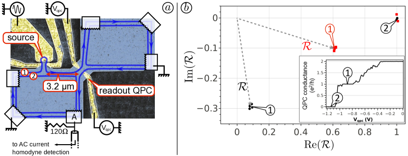
(a) Schematic illustration of the experiment based on the SEM picture of the sample. The two edge states of filling factor are depicted in blue. A mesoscopic capacitor used as the source is capacitively coupled to the outer channel only, and the EMP is generated by a sine drive of variable frequency . The source is placed m before a quantum point contact whose reflection can be varied so as to enable selective readout of the current in both edge states. The figure shows the setup in configuration 1 when channel 2 only is reflected. (b) Ratio for MHz (black dots) and 5500 MHz (red squares) in the complex plane. The principle of measurement is illustrated : is calculated from the ratio of the total current measured in configuration 2 and the current in the inner channel (configuration 1). The grey arrow is the complex vector representing in the complex plane. (Inset) DC measurement of the conductance of the QPC, as a function of the gate voltage , illustrating configuration 1 and 2.
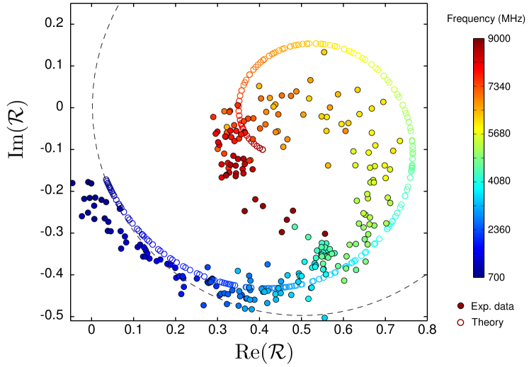
Complex ratio in the complex plane. The color code indicates the frequency of the excited EMP. Experimental data (colored dots) are compared with simulations. The grey dashes show a simulation of both short and long range model, without relaxation. Colored hollow circles present a simulation of the long range model with relaxation, for parameters ps, ps (such that ps), and ps.
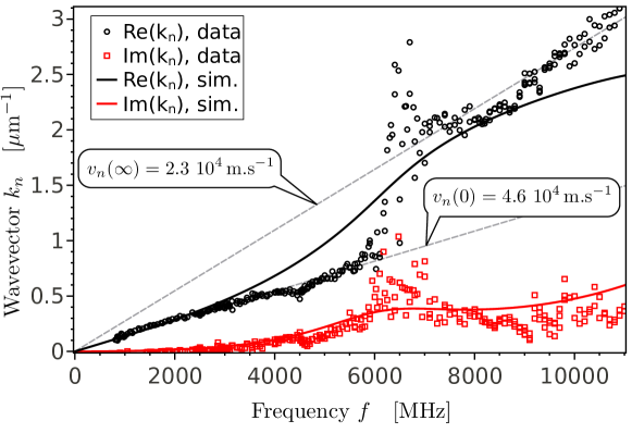
Real and imaginary parts of the wave vector . exhibits two non-dispersive regimes: at low frequency ( GHz), m.s-1, whereas at high frequency ( GHz), m.s-1. indicates damping. Simulations (in black and red line) are proposed with parameters ps, ps ( ps), and ps.
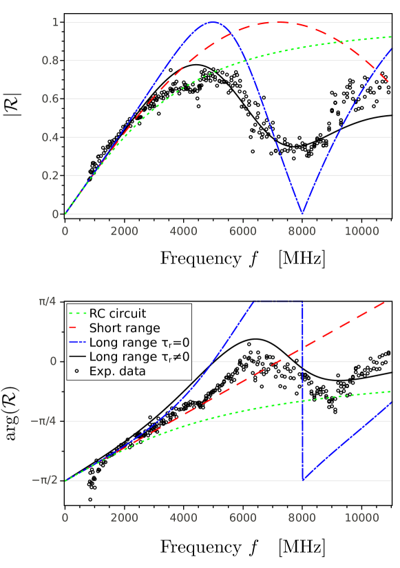
and as a function of drive frequency . Experimental data (black circles) are compared with RC-circuit (green small dashes), short range model (red dashes), long range model without damping (blue dash-dotted line), long range model with relaxation (black plain line). Parameters used are ps, ps ( ps), and ps.
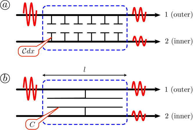
For the zero range model (a), the charge densities are locally coupled to the electrostatic potential by the capacitance matrix per unit length, . For the long range model (b), the potential in each edge is supposed to be uniform and coupled to the total charges by the capacitance matrix
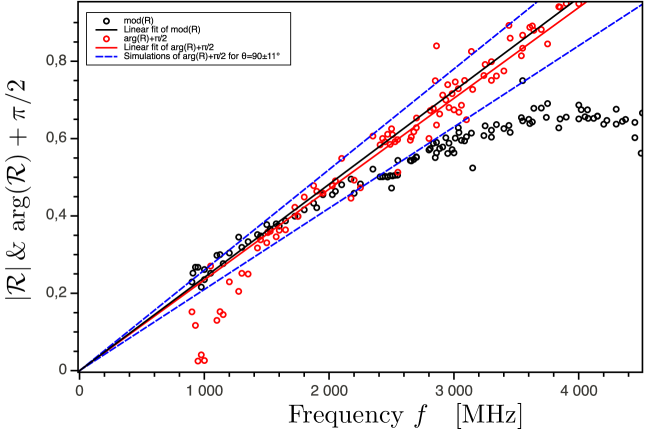
In the low-frequency regime, and are presented respectively in black and red circles, and fitted with linear functions (black and red lines). The slope of is obtained with a accuracy, defining two bounds drawn in blue dashes associated to for and . Data points fall between these bounds confirming .