On the connection between the intergalactic medium and galaxies: The H i–galaxy cross-correlation at $z\lesssim 1$

Abstract

We present a new optical spectroscopic survey of $1777$ ‘star-forming’ (‘SF’) and $366$ ‘non-star-forming’ (‘non-SF’) galaxies at redshifts $z\sim 0-1$ ($2143$ in total), $22$ AGN and $423$ stars, observed by instruments such as DEIMOS, VIMOS and GMOS, in $3$ fields containing $5$ quasi-stellar objects with HST ultra-violet (UV) spectroscopy. We also present a new spectroscopic survey of $165$ ‘strong’ ($10^{14}\leq N_{\rm HI}\lesssim 10^{17}$  cm^-2), and $489$ ‘weak’ ($10^{13}\lesssim N_{\rm HI}<10^{14}$  cm^-2) intervening H i () absorption line systems at $z\lesssim 1$ ($654$ in total), observed in the spectra of $8$ QSOs at $z\sim 1$ by COS and FOS on the HST. Combining these new data with previously published galaxy catalogs such as VVDS and GDDS, we have gathered a sample of $654$ H i absorption systems and $17509$ galaxies at transverse scales $\lesssim 50$  Mpc, suitable for a two-point correlation function analysis. We present observational results on the H i–galaxy ($\xi_{\rm ag}$) and galaxy–galaxy ($\xi_{\rm gg}$) correlations at transverse scales $r_{\perp}\lesssim 10$  Mpc, and the H i–H i auto-correlation ($\xi_{\rm aa}$) at transverse scales $r_{\perp}\lesssim 2$  Mpc. The two-point correlation functions are measured both along and transverse to the line-of-sight, $\xi(r_{\perp},r_{\parallel})$. We also infer the shape of their corresponding ‘real-space’ correlation functions, $\xi(r)$, from the projected along the line-of-sight correlations, assuming power-laws of the form $\xi(r)=(r/r_{0})^{-\gamma}$. Comparing the results from $\xi_{\rm ag}$, $\xi_{\rm gg}$ and $\xi_{\rm aa}$, we constrain the H i–galaxy statistical connection, as a function of both H i column density and galaxy star-formation activity. Our results are consistent with the following conclusions: (i) the bulk of H i systems on $\sim$ Mpc scales have little velocity dispersion ($\lesssim 120$ ) with respect to the bulk of galaxies (i.e. no strong galaxy outflow/inflow signal is detected); (ii) the vast majority ($\sim 100\%$) of ‘strong’ H i systems and ‘SF’ galaxies are distributed in the same locations, together with $75\pm 15\%$ of ‘non-SF’ galaxies, all of which typically reside in dark matter haloes of similar masses; (iii) $25\pm 15\%$ of ‘non-SF’ galaxies reside in galaxy clusters and are not correlated with ‘strong’ H i systems at scales $\lesssim 2$  Mpc; and (iv) $>50\%$ of ‘weak’ H i systems reside within galaxy voids (hence not correlated with galaxies), and are confined in dark matter haloes of masses smaller than those hosting ‘strong’ systems and/or galaxies. We speculate that H i systems within galaxy voids might still be evolving in the linear regime even at scales $\lesssim 2$  Mpc.

1 Introduction

1.1 Motivation

The physics of the intergalactic medium (IGM) and its connection with galaxies are key to understanding the evolution of baryonic matter in the Universe. This is because of the continuous interplay between the gas in the IGM and galaxies: (i) galaxies are formed by the condensation and accretion of primordial or enriched gas; and (ii) galaxies enrich their haloes and the IGM via galactic winds and/or merger events.

Theoretical analyses—under a $\Lambda$ cold dark matter paradigm ($\Lambda$CDM)—suggest that: (i) the accretion happens in two major modes: ‘hot’ and ‘cold’ (e.g. Rees & Ostriker, 1977; White & Rees, 1978; White & Frenk, 1991; Kereš et al., 2005; van de Voort et al., 2011); and (ii) galactic winds are mostly driven by supernova (SN) and/or active galactic nuclei (AGN) feedback (e.g. Baugh et al., 2005; Bower et al., 2006; Lagos, Cora & Padilla, 2008; Creasey, Theuns & Bower, 2013).

Models combining ‘N-body’ dark matter simulations (collisionless, dissipationless) with ‘semi-analytic’ arguments (e.g. Baugh, 2006, and references therein) have been successful in reproducing basic statistical properties of luminous galaxies (e.g. luminosity functions, clustering, star-formation histories, among others). However, in order to provide predictions for the signatures of ‘hot’/‘cold’ accretion and/or AGN/SN feedback in the IGM, a full hydrodynamical description is required.

In practice, hydrodynamical simulations still rely on unresolved ‘sub-grid physics’ to lower the computational cost (e.g. Schaye et al., 2010; Scannapieco et al., 2012), whose effects are not fully understood. Therefore, observations of the IGM and galaxies in the same volume are fundamental to testing these predictions and helping to discern between different physical models (e.g. Fumagalli et al., 2011; Oppenheimer et al., 2012; Stinson et al., 2012; Hummels et al., 2013; Ford et al., 2013; Rakic et al., 2013).

Although the IGM is the main reservoir of baryons at all epochs (e.g. Fukugita, Hogan & Peebles, 1998; Cen & Ostriker, 1999; Schaye, 2001; Davé et al., 2010; Shull, Smith & Danforth, 2012), its extremely low densities make its observation difficult and limited. Currently, the only feasible way to observe the IGM is through intervening absorption line systems in the spectra of bright background sources, limiting its characterization to being one-dimensional. Still, an averaged three dimensional picture can be obtained by combining multiple lines-of-sight (LOS) and galaxy surveys, which is the approach adopted in this work (see Section 1.2).

The advent of the Cosmic Origins Spectrograph (COS) on the Hubble Space Telescope (HST) has revolutionized the study of the IGM and its connection with galaxies at low-$z$ ($z\lesssim 1$). With a sensitivity $\sim 10$ times greater than that of its predecessors, COS has considerably increased the number of QSOs for which UV spectroscopy is feasible. This capability has been exploited for studies of the so-called circumgalactic medium (CGM), by characterizing neutral hydrogen (H i) and metal absorption systems in the vicinity of known galaxies (e.g. Tumlinson et al., 2011; Thom et al., 2012; Werk et al., 2013; Stocke et al., 2013; Keeney et al., 2013; Lehner et al., 2013).

Studies of the CGM implicitly assume a direct one-to-one association between absorption systems and their closest observed galaxy, which might not always hold because of incompleteness in the galaxy surveys and projection effects. Given that metals are formed and expelled by galaxies, a direct association between them seems sensible, in accordance with predictions from low-$z$ simulations (e.g. Oppenheimer et al., 2012). However, the situation for neutral hydrogen is more complicated, as H i traces both enriched and primordial material.

The nature of the relationship between H i and galaxies at low-$z$ has been widely debated. Early studies have pointed out two distinct scenarios for this connection: (i) a one-to-one physical association because they both belong to the same dark matter haloes (e.g. Mo & Morris, 1994a; Lanzetta et al., 1995; Chen et al., 1998); and (ii) an indirect association because they both trace the same underlying dark matter distribution but not necessarily the same haloes (e.g. Morris et al., 1991, 1993; Mo & Morris, 1994b; Stocke et al., 1995; Tripp, Lu & Savage, 1998). More recent studies have shown the presence of H i absorption systems within galaxy voids (e.g. Grogin & Geller, 1998; Penton, Stocke & Shull, 2002; Manning, 2002; Stocke et al., 1995; Tejos et al., 2012), hinting at a third scenario: (iii) the presence of H i absorption systems that are not associated with galaxies (although see Wakker & Savage, 2009).

If we think of galaxies as peaks in the density distribution (e.g. Press & Schechter, 1974), it is natural to expect high column density H i systems to show a stronger correlation with galaxies than low column density ones, owing to a density-H i column density proportionality (e.g. Schaye, 2001; Davé et al., 2010; Tepper-García et al., 2012). Similarly, we also expect the majority of low column density H i systems to belong to dark matter haloes that did not form galaxies. Thus, the relative importance of these three scenarios should depend, to some extent, on the H i column density. Tejos et al. (2012) estimated that these three scenarios account for $\sim 15\%$, $\sim 55\%$ and $\sim 30\%$ of the low-$z$ H i systems at column densities $N_{\rm HI}\gtrsim 10^{12.5}$  cm^-2, respectively, indicating that the vast majority of H i absorption line systems are not physically associated with luminous galaxies (see also Prochaska et al., 2011b, for a similar conclusion).

1.2 Study strategy

In this paper we address the statistical connection between H i and galaxies at $z\lesssim 1$ through a clustering analysis (e.g. Morris et al., 1993; Ryan-Weber, 2006; Wilman et al., 2007; Chen & Mulchaey, 2009; Shone et al., 2010), without considering metals. We focus only on hydrogen because it is the best IGM tracer for a statistical study. Apart from the fact that it traces both primordial and enriched material, it is also the most abundant element in the Universe. Hence, current spectral sensitivities allow us to find H i inside and outside galaxy haloes, which is not the case yet for metals at low-$z$ (according to recent theoretical results; e.g. Oppenheimer et al., 2012).

Focusing on the second half of the history of the Universe ($z\lesssim 1$) has the advantage of allowing relatively complete galaxy surveys even at faint luminosities ($\lesssim L^{*}$; elusive at higher redshifts). Faint galaxies are important for statistical analyses as they dominate the luminosity function, not just in number density, but also in total luminosity and mass. Moreover, the combined effects of structure formation, expansion of the Universe, and the reduced ionization background, allow us to observe a considerable amount of H i systems and yet resolve the so-called H i -forest into individual lines (e.g. Theuns, Leonard & Efstathiou, 1998; Davé et al., 1999). This makes it possible to recover column densities and Doppler parameters through Voigt profile fitting.

One major advantage of clustering over one-to-one association analyses is that it does not impose arbitrary scales, allowing us to obtain results for both small ($\lesssim 1$  Mpc) and large scales ($\gtrsim 1-10$  Mpc). In this way, we can make use of all the H i and galaxy data available, and not only those lying close to each other. Results from the small scale association are important to constraint the ‘sub-grid physics’ adopted in current hydrodynamical simulations. Conversely, results from the largest scales provide information unaffected by these uncertain ‘sub-grid physics’ assumptions (e.g. Hummels et al., 2013; Ford et al., 2013; Rakic et al., 2013). Moreover, the physics and cosmic evolution of the diffuse IGM (traced by H i) obtained by cosmological hydrodynamical simulations (e.g. Paschos et al., 2009; Davé et al., 2010) are in good agreement with analytic predictions (e.g. Schaye, 2001). Our results will be able to test all of these predictions.

Another advantage to using a clustering analysis is that it properly takes into account the selection functions of the surveys. Even at scales $\lesssim 300$  kpc (the typical scale adopted for the CGM), a secure or unique H i–galaxy one-to-one association is not always possible. This is because H i and galaxies are clustered at these scales and because surveys are never $100\%$ complete. Clustering provides a proper statistical description, at the cost of losing details on the physics of an individual H i–galaxy pair. Thus, both one-to-one associations and clustering results are complementary, and needed, to fully understand the relationship between the IGM and galaxies.

In this paper we present observational results for the H i–galaxy two-point correlation function at $z\lesssim 1$. Combining data from UV HST spectroscopy of 8 QSOs in 6 different fields, with optical deep multi-object spectroscopy (MOS) surveys of galaxies around them, we have gathered a sample of $669$ well identified intervening H i absorption systems and $17509$ galaxies at projected separations $\lesssim 50$  Mpc from the QSO line-of-sight (LOS). This dataset is the largest sample to date for such an analysis.

Comparing the results from the H i–galaxy cross-correlation with the H i–H i and galaxy–galaxy auto-correlations, we provide constraints on their statistical connection as a function of both H i column density and galaxy star-formation activity.

Our paper is structured as follows. Sections 2 and 3 describe the IGM and galaxy data used in this work, respectively. The IGM sample is described in Section 4 while the galaxy sample is described in Section 5. Section 6 describes the formalisms used to measure the H i–galaxy cross-correlation and the H i–H i and galaxy–galaxy auto-correlations. Our observational results are presented in Section 7 and discussed in Section 8. A summary of the paper is presented in Section 9.

All distances are in co-moving coordinates assuming $H_{0}=70$ Mpc^-1, $\Omega_{\rm m}=0.3$, $\Omega_{\rm\Lambda}=0.7$, $k=0$, unless otherwise stated, where $H_{0}$, $\Omega_{\rm m}$, $\Omega_{\rm\Lambda}$ and $k$ are the Hubble constant, mass energy density, ‘dark energy’ density and spatial curvature, respectively. Our chosen cosmological parameters lie between the latest results from the Wilkinson Microwave Anisotropy Probe (Komatsu et al., 2011) and the Planck satellite (Planck Collaboration et al., 2013).

Table 1: Properties of the observed QSOs.

QSO Name	Field Name	R.A.	Dec.	$z_{\rm QSO}$	Magnitude
		(hr min sec)	(deg min sec)		Visual (Band)	NUV (AB)	FUV (AB)
(1)	(2)	(3)	(4)	(5)	(6)	(7)	(8)
Q0107-025A	Q0107	01 10 13.10	$-$02 19 52.0	0.96000	18.1 ($B$)	18.1	19.3
Q0107-025B	Q0107	01 10 16.20	$-$02 18 50.0	0.95600	17.4 ($V$)	17.5	18.6
Q0107-0232	Q0107	01 10 14.51	$-$02 16 57.5	0.72600	18.4 ($B$)	18.9	20.1
J020930.7-043826	J0209	02 09 30.74	$-$04 38 26.3	1.12800	17.2 ($g$)	17.5	18.5
J100535.24+013445.7	J1005	10 05 35.26	$+$01 34 45.6	1.08090	16.8 ($g$)	17.4	18.6
J102218.99+013218.8	J1022	10 22 18.99	$+$01 32 18.8	0.78900	16.8 ($V$)	17.2	18.1
J135726.27+043541.4	J1357	13 57 26.27	$+$04 35 41.4	1.23176	17.2 ($g$)	17.8	19.2
J221806.67+005223.6	J2218	22 18 06.69	$+$00 52 23.7	1.27327	17.8 ($V$)	18.6	24.0

(1) Name of the QSO. (2) Name of the field. (3) Right ascension (J2000). (4) Declination (J2000). (5) Redshift of the QSO. (6) Apparent visual magnitude; the band is given in parenthesis. (7) Apparent near-UV magnitude from GALEX. (8) Apparent far-UV magnitude from GALEX.

^a The sudden decrease in flux is due to the presence of a Lyman Limit System.

Table 2: Summary of the QSO observations (HST spectroscopy).

QSO Name	Instrument	Grating	Wavelength	FWHM	Dispersion	$\langle S/N\rangle$	Exposure	Program ID
			range (Å)	(Å)	(Å/pixel)	(per pixel)	time (h)
(1)	(2)	(3)	(4)	(5)	(6)	(7)	(8)	(9)
Q0107-025A	COS	G130M	1135–1460	0.07	0.01	9	7.8	11585
	COS	G160M	1460–1795	0.09	0.01	8	12.3	11585
	FOS	G190H	1795–2310	1.39	0.36	28	7.5	5320, 6592
	FOS	G270H	2310–3277	1.97	0.51	32	2.4	6100
Q0107-025B	COS	G130M	1135–1460	0.07	0.01	9	5.9	11585
	COS	G160M	1460–1795	0.09	0.01	7	5.9	11585
	FOS	G190H	1795–2310	1.39	0.36	28	1.8	5320, 6592
	FOS	G270H	2310–3277	1.97	0.51	32	1.8	6100
Q0107-0232	COS	G160M	1434–1795	0.09	0.01	7	23.2	11585
	FOS	G190H	1795–2310	1.39	0.36	18	9.1	11585
J020930.7-043826	COS	G130M	1277–1460	0.07	0.01	12	3.9	12264
	COS	G160M	1460–1795	0.09	0.01	10	7.8	12264
	COS	G230L	1795–3084	0.79	0.39	12	4.0	12264
J100535.24+013445.7	COS	G130M	1135–1460	0.07	0.01	9	3.9	12264
	COS	G160M	1460–1795	0.09	0.01	9	6.2	12264
J102218.99+013218.8	COS	G130M	1135–1460	0.07	0.01	6	0.6	11598
	COS	G160M	1460–1795	0.09	0.01	5	0.8	11598
J135726.27+043541.4	COS	G130M	1135–1460	0.07	0.01	9	3.9	12264
	COS	G160M	1460–1795	0.09	0.01	7	7.8	12264
	COS	G230L	1795–3145	0.79	0.39	11	4.0	12264
J221806.67+005223.6	COS	G230L	2097–3084	0.79	0.39	10	5.6	12264

(1) Name of the QSO. (2) Instrument. (3) Grating. (4) Wavelength range used for a given setting. (5) Full-width at half maximum of the line spread function of the spectrograph. (6) Dispersion. (7) Average signal-to-noise ratio per pixel over the given wavelength range. (8) Exposure time of the observations. (9) HST program ID of the observations.

^a Due to the presence of a Lyman Limit System blocking shorter wavelengths.

^b Due to poor signal-to-noise data at shorter wavelengths.

2 Intergalactic medium data

We used HST spectroscopy of 8 QSOs to characterize the diffuse IGM through the observations of intervening H i absorption line systems. We used data from COS (Green et al., 2012) taken under HST programs General Observer (GO) 12264 (PI: Morris), GO 11585 (PI: Crighton) and GO 11598 (PI: Tumlinson); and data from the Faint Object Spectrograph (FOS) (Keyes et al., 1995) taken under HST programs GO 5320 (PI: Foltz), GO 6100 (PI: Foltz) and GO 6592 (PI: Foltz).

Data from program GO 12264 were taken to study the statistical relationship between H i absorption line systems and galaxies at redshift $z\lesssim 1$. We selected four QSOs at $z_{\rm QSO}\sim 1$ (namely J020930.7-043826, J100535.24+013445.7, J135726.27+043541.4 and J221806.67+005223.6) lying in fields of view that were already surveyed for their galaxy content by the Deep Survey (VVDS) (Le Fèvre et al., 2005; Le Fevre et al., 2013) and the Gemini Deep Deep Survey (GDDS) (Abraham et al., 2004). Data from programs GO 5320, GO 6100, GO 6592 and GO 11585 contain spectroscopy of three QSOs (namely Q0107-025A, Q0107-025B and Q0107-0232) whose LOSs are separated by $\sim 0.4-1$  Mpc. This triple QSO field is ideal for measuring the characteristic sizes of the H i absorption systems but it can also be used to address the connection between H i systems and galaxies (e.g. Crighton et al., 2010). Data from program GO 11598 were originally taken to investigate the properties of the CGM by targeting QSOs whose LOS lie within $\lesssim 150$  kpc of a known galaxy. For this paper we used one QSO observed under program GO 11598 (namely J102218.99+013218.8), for which we have conducted our own galaxy survey around its LOS (see Section 3). Given that this LOS contains only one pre-selected galaxy, this selection will not affect our results on the IGM–galaxy statistical connection.

Table 1 summarizes our QSO sample while Table 2 gives details on their HST observations.

2.1 Data reduction

2.1.1 COS data

Individual exposures from COS were downloaded from the Space Telescope Science Institute (STScI) archive and reduced using calcos v2.18.5 in combination with Python routines developed by the authors. A full description of the reduction process will be presented in Finn et al. (2013, in prep.), here we present a summary.

Individual files corresponding to single central wavelength setting, stripe and FP-POS (i.e. x1d files) were obtained directly from calcos. The source extraction was performed using a box of 25 pixels wide along the spatial direction for all G130M exposures, and 20 pixels for all G160M and G230L exposures. The background extraction was performed using boxes encompassing as much of the background signal as possible, whilst avoiding regions close to the detector edges. We set the background smoothing length in calcos to $1$ pixel and performed our own background smoothing procedure masking out portions of the spectra affected by strong geocoronal emission lines (namely the H i and O 1 $\lambda\lambda 1302,1306$) and pixels with bad data quality flags. We interpolated across the gaps to get the background level in these excluded regions. The background smoothing lengths were set to 1000 pixels for the far ultra-violet (FUV)A stripes, 500 pixels for the FUVB stripes and 100 pixels for all near ultra-violet (NUV) stripes, along the dispersion direction.

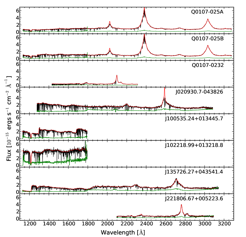
Figure 1: Observed spectra of our sample of QSOs: flux (black lines), uncertainty (multiplied by a factor of $5$ for clarity; green lines) and continuum fit (red lines). Wavelengths $\lambda<1795$ Å and $\lambda\geq 1795$ Å correspond to data from the FUV and NUV channels respectively (see Table 2). The FUV spectra have been re-binned to match the resolution of the NUV spectra for clarity.

The error array was calculated in the same way as in calcos, but using our new background estimation. Each spectrum was then flux calibrated using sensitivity curves provided by STScI.

Co-alignment was performed by cross-correlating regions centred on strong Galactic absorption features (namely, C 2 $\lambda 1334$, Al 2 $\lambda 1670$, Si 2 $\lambda 1260$, Si 2 $\lambda 1526$ and Mg 2 $\lambda\lambda 2796,2803$ Å). For each grating we pick the central wavelength setting and FP-POS position with the most accurately determined wavelength solutions from STScI as a reference. These are FP-POS $=3$ for all gratings, central wavelengths of $1309$ and $1600$ Å for the G130M and G160M gratings respectively, and $2950$ Å (using only the ‘B’ stripe) for the G230L grating. All other settings for each grating are then cross-correlated on these ones, assuming the reference and comparison settings both contain one of the absorption features specified. Wavelengths offsets are then applied to the comparison settings to match the reference ones. These offsets typically amount to a resolution element or less. For those settings that could not be aligned on any of the Galactic features specified, we manually searched for other strong absorption lines on which to perform the cross-correlation. Strong absorption lines were always found. We then scaled the fluxes of the comparison setting such that its median flux value matches that of either the reference or the already calibrated setting in the overlapped region.

At this point we changed some pixel values according to their quality flags: flux and error values assigned to pixels with bad data quality flags were set to zero, while pixels with warnings had their exposure times reduced by a factor of two. We then re-scaled the wavelength binning of each exposure to have a constant spacing equal to the dispersion for the grating, using nearest-neighbour interpolation. The combined wavelength binning therefore consists of three wavelength scales, one for the G130M grating ($\lambda<1460$ Å), one for the G160M grating ($1460\leq\lambda<1795$ Å) and one for the G230L grating ($\lambda\geq 1795$Å).

The co-addition was then performed via modified exposure time weighting. Finally, the combined FUV and NUV spectra were re-binned to ensure Nyquist sampling (two pixels per resolution element). Both are binned onto a linear wavelength scale with spacing equal to 0.0395 Å for the FUV, and a spacing equal to 0.436 Å for the NUV.

2.1.2 FOS data

Individual exposures from FOS were downloaded from the STScI archive and reduced using the standard calfos pipeline. Wavelength corrections given by Petry et al. (2006) were applied to each individual exposure. As described by Petry et al., these corrections were determined using a wavelength calibration exposure taken contemporaneously with the G190H grating science exposures, and were verified using Galactic Al 2 and Al 3 absorption features. The shortest wavelength region of the FOS G190H settings overlap with the longest wavelength COS settings, and we confirmed that the wavelength scales in these overlapping regions were consistent between the two instruments. Then we combined all individual exposures together, resampling to a common wavelength scale of $0.51$ Å per pixel.

2.2 Continuum fitting

We fit the continuum of each QSO in a semi-automatized and iterative manner: (i) we first divide each spectrum in multiple chunks, typically of $12$ Å at wavelengths shorter than that of the H i  emission from the QSOs (at larger wavelengths we used much longer intervals but these are not relevant for the present work); (ii) we then fit straight line segments through the set of points given by the central wavelength and the median flux values for each chunk; (iii) we then removed pixels with flux values falling $3\times$ their uncertainty below the fit value; (iv) we repeat steps (ii) and (iii) until a converged solution is reached; (v) we fit a cubic spline through the final set of median points to get a smooth continuum. The success of this method strongly depends on the presence of emission lines, and on number and positions of the chosen wavelength chunks. Therefore, we visually inspect the solution and improve it by adding and/or removing points accordingly, making sure that the distribution of flux values above the continuum fit is consistent with a Gaussian tail. We checked that the use of these subjective steps does not affect the final results significantly (see Section 4.4).

In Figure 1 we show our QSO spectra (black lines) with their corresponding uncertainties (green lines) and continuum fit (red lines). We refer the reader to Finn et al. (2013, in prep.) for further details on the continuum fitting process (including the continuum fit associated to the peaks of the broad emission lines).

3 Galaxy data

Table 3: Summary of galaxy observations (spectroscopy).

Field Name	Instrument	Gratting	Wavelength	Dispersion	Exposure	Reference
			range (Å)	(Å/pixel)	time (h)
(1)	(2)	(3)	(4)	(5)	(6)	(7)
Q0107	DEIMOS	1200l/mm	6400-9100	0.3	0.99	This paper
	GMOS	R400	5000-9000	0.7	0.90	This paper
	VIMOS	LR_red	5500-9500	7.3	0.96	This paper
	CFHT-MOS	O300	5000-9000	3.5	0.83	Morris & Jannuzi (2006)
J0209	GMOS	R150_G5306	5500-9200	3.4	21	GDDS
J1005	VIMOS	LR_red	5500-9500	7.3	0.96	This paper
	VIMOS	LR_red	5500-9500	7.3	0.83	VVDS
J1022	VIMOS	LR_red	5500-9500	7.3	0.96	This paper
J1357	VIMOS	LR_red	5500-9500	7.3	0.83	VVDS
J2218	VIMOS	LR_red	5500-9500	7.3	0.96	This paper
	VIMOS	LR_red	5500-9500	7.3	0.83	VVDS

(1) Name of the field. (2) Instrument. (3) Gratting. (4) Wavelength range. (5) Dispersion. (6) Exposure time of the observations. (7) Reference of the observations.

^a Redshift uncertainties for each instrument setup are described in Section 3.

Our chosen QSOs are at $z_{\rm QSO}\sim 0.7-1.3$, so we aim to target galaxies at $z\lesssim 1$, corresponding to the last $\sim 7$ Gyr of cosmic evolution. The majority of these QSOs lie in fields already surveyed for their galaxy content. We used archival galaxy data from: the VVDS (Le Fèvre et al., 2005; Le Fevre et al., 2013), GDDS (Abraham et al., 2004) and the Canada France Hawaii Telescope (CFHT) MOS survey published by Morris & Jannuzi (2006). Despite the existence of some galaxy data around our QSO fields we have also performed our own galaxy surveys using MOS to increase the survey completeness. We acquired new galaxy data from different ground-based MOS, namely: the Visible Multi-Object Spectrograph (VIMOS) (Le Fèvre et al., 2003) on the VLT under programs 086.A-0970 (PI: Crighton) and 087.A-0857 (PI: Tejos); the Deep Imaging Multi-Object Spectrograph (DEIMOS) (Faber et al., 2003) on Keck under program A290D (PIs: Bechtold and Jannuzi); and the Gemini Multi-Object Spectrograph (GMOS) (Davies et al., 1997) on Gemini under program GS-2008B-Q-50 (PI: Crighton). Table 3 summarizes the observations taken to construct our galaxy samples.

The following sections provide detailed descriptions of the observations, data reduction, selection functions and construction of our new galaxy samples. We also give information on the subsamples of the previously published galaxy surveys used in this work.

3.1 VIMOS data

3.1.1 Instrument setting

We used the low-resolution (LR) grism with 1.0 arcsecond slits ($R\equiv\lambda/\Delta\lambda\approx 200$) due to its high multiplex factor in the dispersion direction (up to $4$). As we needed to target galaxies up to the QSOs redshifts ($z_{\rm{QSO}}\sim 0.7-1.3$), we used that grism in combination with the OS-red filter giving coverage between $5500-9500$ Å.

3.1.2 Target selection, mask design and pointings

We used $R$-band pre-imaging to observe objects around our QSO fields and sextractor v2.5 (Bertin & Arnouts, 1996) to identify them and assign $R$-band magnitudes, using zero points given by ESO. For fields J1005, J1022 and J2218 we added a constant shift of $\sim 0.38$ magnitudes to match those reported by the VVDS survey in objects observed by both surveys (see Section 3.5.2 and Figure 4). No correction was added to the Q0107 field. For objects in fields J1005, J1022 and J2218 we targeted objects at $R<23.5$, giving priority to those with $R<22.5$. For objects in field Q0107 we targeted objects at $R<23$, giving priority to those with $R<22$. We did not impose any morphological star/galaxy separation criteria, given that unresolved galaxies will look like point sources (see Section 5.3). The masks were designed using the vmmps (Bottini et al., 2005) using the ‘Normal Optimization’ method (random) to provide a simple selection function. We targeted typically $\sim 70-80$ objects per mask per quadrant, equivalent to $\sim 210-320$ objects per pointing. We used three pointings of one mask each, shifted by $\sim 2.5$ arcminutes centred around the QSO.

3.1.3 Data reduction for field Q0107

The spectroscopic data were taken in 2011 and the reduction was performed using vipgi (Scodeggio et al., 2005) using standard parameters. We took three exposures per pointing of $1155$ s, followed by lamps. The images were bias corrected and combined using a median filter. Wavelength calibration was performed using the lamp exposures, and further corrected using five skylines at $5892$, $6300$, $7859$, $8347$ and $8771$ Å (Osterbrock et al., 1996; Osterbrock, Fulbright & Bida, 1997). Finally, the slits were spectrophotometrically calibrated using standard star spectra (Oke, 1990; Hamuy et al., 1992, 1994) taken at dates similar to our observations. The extraction of the one-dimensional (1D) spectra was performed by collapsing objects along the spatial axis, following the optimal weighting algorithm presented in Horne (1986). Our wavelength solutions per slit show a quadratic mean $rms\lesssim 1$ Å in more than $75\%$ of the slits and a $rms\lesssim 2$ Å in all the cases. We consider these as good solutions, given that the pixel size for the low resolution mode is $\sim 7$ Å. These data were taken before the recent update of the VIMOS charge-coupled devices on August 2010, and so fringing effects considerably affected the quality of the data at $\gtrsim 7500$ Å. We attempted to correct for this with no success.

3.1.4 Data reduction for fields J1005, J1022 and J2218

The spectroscopic data were taken on 2011 and the reduction was performed using esorex v.3.9.6. All three pointings of fields J1005 and J1022 were observed, while only ‘pointing 3’ of J2218 was observed. Due to a problem with focus, data from ‘quadrant 3’ of ‘pointing 1’ and ‘pointing 3’ of field J1022 were not usable. ‘Pointing 2’ (middle one) of fields J1005 and J1022 were observed twice to empirically asses the redshift uncertainty (see Section 3.1.5). We took three exposures per pointing of 1155 s followed by lamps. The reduction was performed using a peakdetection parameter (threshold for preliminary peak detection in counts) of $500$ when possible, and decreasing it when needed to minimize the number of slits lost (we typically lost $\sim 1$ slit per quadrant). We also set the cosmics parameter to ‘True’ (cleaning cosmic ray events) and stacked our 3 images using the median. Wavelength calibration was further improved using four skylines at $5577.34$, $6300.30$, $8827.10$ and $9375.36$ Å (Osterbrock et al., 1996; Osterbrock, Fulbright & Bida, 1997) with the skyalign parameter set to 1 (1st order polynomial fit to the expected positions). The slits were spectrophotometrically calibrated using standard star spectra (Oke, 1990; Hamuy et al., 1992, 1994) taken at dates similar to our observations. The extraction of the one-dimensional (1D) spectra was performed by collapsing the objects along the spatial axis, following the optimal weighting algorithm presented in Horne (1986). Our wavelength solutions per slit show a quadratic mean $rms\lesssim 1$ Å in more than $90\%$ of the cases, which we considered as satisfactory for a pixel size of $\sim 7$ Å. These data were taken after a recent update to the VIMOS CCDs on August 2010, and so no important fringing effects were present.

3.1.5 Redshift determination

Redshifts for our new galaxy survey were measured by cross-correlating galaxy, star, and QSO templates with each observed spectrum. We used templates from the Sloan Digital Sky Survey (SDSS) degraded to the lower resolution of our VIMOS observations. Galaxy templates were redshifted from $z=0$ to $z=2$ using intervals of $\Delta z=0.001$. The QSO template was redshifted between $z=0$ to $z=4$ using larger intervals of $\Delta z=0.01$. Star templates were shifted $\pm 0.005$ around $z=0$ using intervals of $\Delta z=0.0001$ to help improve the redshift measurements and quantify the redshift uncertainty (see below). We improved the redshift solution by fitting a parabola to the $3$ redshift points with the largest cross-correlation values around each local maximum. This technique gives comparable redshift solutions (within the expected errors) to that obtained by decreasing the redshift intervals by a factor $\sim 10$, but at a much lower computational cost. Before computing the cross-correlations, we masked out regions at the very edges of the wavelength coverage ($<5710$ and $>9265$ Å) and those associated with strong sky emission/absorption features (between $5870-5910$, $6275-6325$ and $7550-7720$ Å). For the Q0107 field we additionally masked out the red part at $>7550$ Å because of fringing problems. We visually inspected each 1-dimensional and 2-dimensional spectrum and looked for the ‘best’ redshift solution (see below).

3.1.6 Redshift reliability

For each targeted object we manually assigned a redshift reliability flag. We used a very simple scheme based on three labels: ‘a’ (‘secure’), ‘b’ (‘possible’) and ‘c’ (‘uncertain’). As a general rule, spectra assigned with ‘a’ flags have at least $3$ well identified spectral features (either in emission or absorption) or $2$ well identified emission lines; spectra assigned with ‘c’ flag are those which do not show clear spectral features either due to a low signal-to-noise ratio or because of an intrinsic lack of such lines observed at the VIMOS resolution (e.g. some possible A, F and G type stars appear in this category); spectra assigned with ‘b’ flags are those that lie in between the two aforementioned categories.

3.1.7 Uncertainty of the semi-automatized process

The process includes subjective steps (determining the ‘best’ template and redshift, and assigning a redshift reliability). This uncertainty was estimated by comparing two sets of redshifts obtained independently by three of the authors (N.T. versus S.L.M. and N.T. versus N.H.M.C.) in two subsamples of the data. We found discrepancies in $\lesssim 5\%$ of the cases, the vast majority of which were for redshifts labelled as ‘b’.

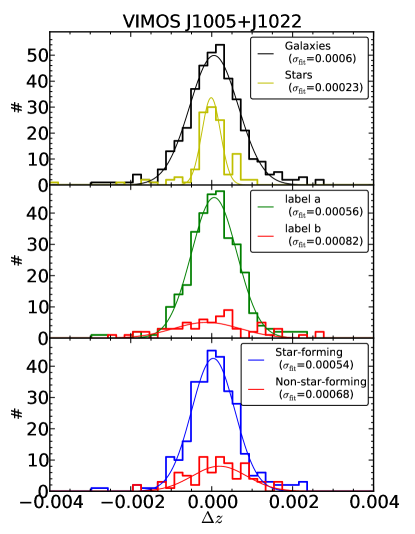
Figure 2: Histograms of the measured redshift difference between two independent observations of a same object in fields J1005 and J1022. Top panel: all identified galaxies (black lines) and stars (yellow lines). Middle panel: galaxies with ‘secure’ redshifts (label ‘a’; green lines) and with ‘possible’ redshifts (label ‘b’; red lines). Bottom panel: galaxies classified as ‘star-forming’ (blue lines) and as ‘non-star-forming’ (red lines; see Section 5.1). Best Gaussian fits to the histograms and standard deviation values are also shown.

3.1.8 Further redshift calibration for fields J1005, J1022 and J2218

Even though the wavelength calibration from the esorex reduction was generally satisfactory, we found a $\sim 1$ pixel systematic discrepancy between the obtained and expected wavelength for some skylines in localized areas of the spectrum (particularly towards the red end). This effect was most noticeable in quadrant 3, where the redshift difference between objects observed twice showed a distribution displaced from zero by $\sim 0.001$ ($\sim 1$ pixel). A careful inspection revealed that the other quadrants also showed a similar but less strong effect ($\lesssim$ 0.5 pixel). We corrected for this effect using the redshift solution of the stars. For a given quadrant we looked at the mean redshift of the stars and applied a systematic shift of that amount to all the objects in that quadrant. This correction placed the mean redshift of stars at zero, and therefore corrected the redshift of all objects accordingly.

3.1.9 Redshift statistical uncertainty for fields J1005, J1022 and J2218

In order to assess the redshift uncertainty for these fields, we measured a redshift difference between two independent observations of the same object. These objects were observed twice, and come mainly from our ‘pointing 2’ in fields J1005 and J1022, but there is also a minor contribution ($\lesssim 10\%$) of objects that were observed twice using different pointings. Figure 2 shows the observed redshift differences for all galaxies and stars (top panel); galaxies with ‘secure’ and ‘possible’ redshifts (middle panel); and galaxies classified as ‘star-forming’ (‘SF’) or ‘non-star-forming’ (‘non-SF’) based on the presence of current, or recent, star formation (see Section 5.1; bottom panel). All histograms are centred around zero and do not show evident systematic biases. The redshift difference of all galaxies show a standard deviation of $\approx 0.0006$. A somewhat smaller standard deviation is observed for galaxies with ‘secure’ redshifts and/or those classified as ‘SF’ (note that there is a large overlap between these two samples), and consequently a somewhat larger standard deviation is observed for galaxies with ‘possible’ redshift and/or classified as ‘non-SF’. This behaviour is of course expected, as it is simpler to measure redshifts for galaxies with strong emission lines (for which the peak in the cross-correlation analysis is also better constrained) than for galaxies with only absorption features (at a similar signal-to-noise ratio). From this analysis we take $\approx 0.0006/\sqrt{2}=0.0004$ as the representative redshift uncertainty of our VIMOS galaxy survey in these fields. This uncertainty corresponds to $\approx 120-60$  at redshift $z=0-1$. This uncertainty is $\sim 2$ times smaller than that claimed for the VVDS survey (Le Fèvre et al., 2005; Le Fevre et al., 2013).

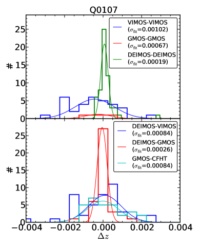
Figure 3: Histograms of the measured redshift difference between two independent observations of the same object in field Q0107. Top panel shows it for galaxies observed twice by the same instrument: VIMOS-VIMOS (blue lines), GMOS-GMOS (red lines) and DEIMOS-DEIMOS (green lines). Bottom panel shows it for objects observed twice by different instruments, after shifting to match the DEIMOS mean: DEIMOS-VIMOS (blue lines), DEIMOS-GMOS (red lines) and GMOS-CFHT (cyan lines). Best Gaussian fits to the histograms and standard deviation values are also shown.

3.1.10 Further redshift calibration for field Q0107

We did not see systematic differences between quadrants, as was seen for fields J1005, J1022 and J2218. VIMOS observations of the Q0107 field were reduced differently, and the data come mainly from the blue part of the spectrum. Therefore, such an effect might not be present or, if present, might be more difficult to detect. However, we did find a systematic shift between the redshifts measured from VIMOS compared to those measured from DEIMOS. Given the much higher resolution of DEIMOS, we used its frame as reference for all our Q0107 observations. Thus, we corrected the Q0107 VIMOS redshifts to match the DEIMOS frame. This correction was $\sim 0.0008$ ($\lesssim 1$ VIMOS pixel) and the result is shown in the bottom panel of Figure 3 (blue lines).

3.1.11 Redshift statistical uncertainty for field Q0107

In order to assess the redshift uncertainty, we used objects that were observed twice in the Q0107 field. We found a distribution of redshift differences centred at $\sim 0$ with a standard deviation of $\approx 0.001$ (see top panel of Figure 3), corresponding to a single VIMOS uncertainty of $\approx 0.001/\sqrt{2}\approx 0.0007$. Another way to estimate the VIMOS uncertainty in the Q0107 field is by looking at the redshift difference for objects that were observed twice, once by VIMOS and another time by DEIMOS (44 in total; see bottom panel of Figure 3). In this case, the distribution shows a standard deviation of $\approx\sqrt{0.00084}$, corresponding to a single VIMOS uncertainty of $\sqrt{0.00084^{2}-0.00013^{2}}\approx 0.0008$, given that the uncertainty of a DEIMOS single measurement is $\approx 0.00013$ (see below). So, we take a value of $\approx 0.00075$ as the representative redshift uncertainty of a single VIMOS observation in the Q0107 field. This uncertainty corresponds to $\approx 220-110$  at redshift $z=0-1$. This uncertainty is larger than that of fields J1005, J1022 and J2218, consistent with the poorer quality detector being used.

3.2 DEIMOS data

3.2.1 Instrument setting

We patterned our DEIMOS observations to resemble the Deep Extragalactic Evolutionary Probe 2 (DEEP2) ‘1 hour’ survey (Coil et al., 2004). We used the $1200$ line mm^-1 grating with a 1.0 arcsecond slit giving a resolution of $R\sim 5000$ over the wavelength range $6400-9100$ Å.

3.2.2 Target selection

We used $B$, $R$ and $I$ bands pre-imaging to select objects around our Q0107 field. We used sextractor v2.5 (Bertin & Arnouts, 1996) to identify them and assign $B$, $R$ and $I$ magnitudes to them. We used color cuts as in Coil et al. (2004, see also ) to target galaxies:

$$\begin{split}B-R&\leq 2.35(R-I)-0.45\ \rm{or}\\ R-I&\geq 1.15\ \rm{or}\\ B−R&\geq 0.5\ \rm{.}\end{split}$$ (1)

We also gave priority to objects within 1 arcminute of the Q0107-025A LOS. We targeted objects up to $R=24.5$ magnitudes, but we assigned higher priorities to the brightest ones. In an attempt to be efficient, we also imposed a star/galaxy morphological criteria of CLASS_STAR$<0.97$ (although see Section 5.3).

3.2.3 Data reduction

The observations were taken in 2007 and 2008. The reduction was performed using the DEEP2 DEIMOS Data Pipeline (Newman et al., 2012), from which galaxy redshifts were also obtained.

3.2.4 Redshift reliability

The redshift reliability for DEIMOS data was originally based on four subjective categories: (0) ‘still needs work’, (1) ‘not good enough’, (2) ‘possible’, (3) ‘good’ and (4) ‘excellent’. In order to have a unified scheme we matched those DEIMOS labels with our previously defined VIMOS ones (see Section 3.1.5) as follows: DEIMOS label 4 is matched to label ‘a’ ({4}$\rightarrow$ {‘a’}); DEIMOS labels 3 and 2 are matched to label ‘b’ ({3,2}$\rightarrow$ {‘b’}); and DEIMOS labels 1 and 0 are matched to label ‘c’ ({1,0}$\rightarrow$ {‘c’}).

3.2.5 Redshift statistical uncertainty for field Q0107

In order to assess the redshift uncertainty, we used objects that were observed twice in the Q0107 field. We found a distribution of redshift differences centred at $\sim 0$ with a standard deviation of $\approx 0.00019$ (see top panel of Figure 3), corresponding to a single DEIMOS uncertainty of $\approx 0.00019/\sqrt{2}\approx 0.00013$. So, we take a value of $\approx 0.00013$ as the representative redshift uncertainty of a single DEIMOS observation in the Q0107 field. This uncertainty corresponds to $\approx 40-20$  at redshift $z=0-1$.

3.3 GMOS data

3.3.1 Instrument setting

We used the R400 grating centred on a wavelength of 7000 Å with a 1.5 arcseconds slit giving a resolution of $R=639$.

3.3.2 Target selection, mask design and pointings

We used $R$-band pre-imaging to select objects around our Q0107 field. We used sextractor v2.5 (Bertin & Arnouts, 1996) to identify objects and assign them $R$-band magnitudes. The masks were designed using gmmps . Top priority was given to objects with $R<22$, followed by those with $22\leq R<23$ and last priority to those with $23\leq R<24$. We typically targeted $\sim 40$ objects per mask. Six masks were taken, three around QSO C, two around QSO B, and one around QSO A, where many objects had already been targeted in previous observations.

3.3.3 Data reduction

The observations were taken in 2008 . Three 1080 s offset science exposures were taken for each mask, dithered along the slit to cover the gaps in the CCD detectors. Arcs were taken contemporaneously to the science exposures. We used the Gemini Image Reduction and Analysis Facility (IRAF) package to reduce the spectra. A flat-field lamp exposure was divided into each bias-subtracted science exposure to remove small-scale variations across the CCDs, and the fringing pattern seen at red wavelengths. The dithered images (both arcs and science) were then combined into a single exposure. The spectrum for each mask was wavelength-calibrated by identifying known arc lines and fitting a polynomial to match pixel positions to wavelengths. Finally the wavelength-calibrated 2-d spectra were extracted to produced 1-d spectra. The typical $rms$ scatter of the known arc line positions around the polynomial fit ranged from 0.5 to 1.0 Å, depending on how many arc lines were available to fit (bluer wavelength ranges tended to have fewer arc lines). A 0.75 Å $rms$ scatter corresponds to a velocity error of 38 at 6000 Å.

3.3.4 Redshift determination and reliability

We determined redshifts by using the same method to that of the VIMOS spectra: plausible redshifts were identified as peaks in the cross-correlation measured between the GMOS spectra and spectral templates (see Section 3.1.5 for further details). Redshifts reliabilities were also assigned following the definitions in our VIMOS sample.

3.3.5 Further redshift calibration

We found a systematic shift of the redshifts measured from GMOS with respect to those measured from DEIMOS for the 40 objects observed by these two instruments. Given the much higher resolution of DEIMOS we used its frame as reference for our Q0107 observations. Thus, we corrected all GMOS redshifts to match the DEIMOS frame. This correction was $\sim 0.0004$ or $\sim 80$ ($\lesssim 1$ GMOS pixel) and the result is shown in the bottom panel of Figure 3 (red lines).

3.3.6 Redshift statistical uncertainty for field Q0107

There were only 3 objects that were observed twice using GMOS (see top panel of Figure 3), and so we did not take the uncertainty from such an small sample. Instead, we use objects observed by both GMOS and DEIMOS to estimate the GMOS redshift uncertainty. The distribution of redshift differences for objects with both GMOS and DEIMOS spectra (see bottom panel of Figure 3) shows a standard deviation of $\approx 0.00027$. Given that the uncertainty of DEIMOS alone is $\approx 0.00013$ we estimate the GMOS uncertainty to be $\approx\sqrt{0.00027^{2}-0.00013^{2}}\approx 0.00024$. This uncertainty corresponds to $\approx 70-35$  at redshift $z=0-1$.

3.4 CFHT MOS data

We used the CFHT galaxy survey of the Q0107 field presented by Morris & Jannuzi (2006). There are $61$ galaxies in this sample, $29$ of which were also observed by our GMOS survey. We use only redshift information from this sample without assigning a particular template or redshift label. We refer the reader to Morris & Jannuzi (2006) for details on the data reduction and construction of the galaxy sample.

3.5 VVDS

Three of the QSOs presented in this paper (namely: J100535.24+013445.7, J135726.27+043541.4 and J221806.67+005223.6) were chosen because they lie in fields already surveyed for galaxies by the VVDS survey (Le Fèvre et al., 2005; Le Fevre et al., 2013). For our purposes, we use a subsample of the whole VVDS survey, selecting only galaxies in those fields. We refer the reader to Le Fèvre et al. (2005) and Le Fevre et al. (2013) for details on the data reduction and construction of these galaxy catalogs.

3.5.1 Redshift reliability

The redshift reliability for VVDS data was originally based on six categories: (0) ‘no redshift’, (1) ‘50% confidence’; (2) ‘75% confidence’; (3) ‘95% confidence’; (4) ‘100% confidence’; (8) ‘single emission line’; and (9) ‘single isolated emission line’ (Le Fèvre et al., 2005; Le Fevre et al., 2013). They expanded this classification system for secondary targets (objects which are present by chance in the slits) by the use of the prefix ‘2’. Similarly the prefix ‘1’ means ‘primary QSO target’, while the prefix ‘21’ means ‘secondary QSO target’. In order to have a unified scheme we matched those VVDS labels with our previously defined VIMOS ones (see Section 3.1.5) as follows: VVDS label 4, 3 and their corresponding extensions are matched to label ‘a’ ({4,14,24,214,3,13,23,213}$\rightarrow$ {‘a’}); VVDS labels 2, 9 and their corresponding extensions are matched to label ‘b’ ({2,12,22,212,9,19,29,219}$\rightarrow$ {‘b’}); and VVDS labels 1, 0 and their corresponding extensions are matched to label ‘c’ ({1,11,21,211,0,10,20,210}$\rightarrow$ {‘c’}).

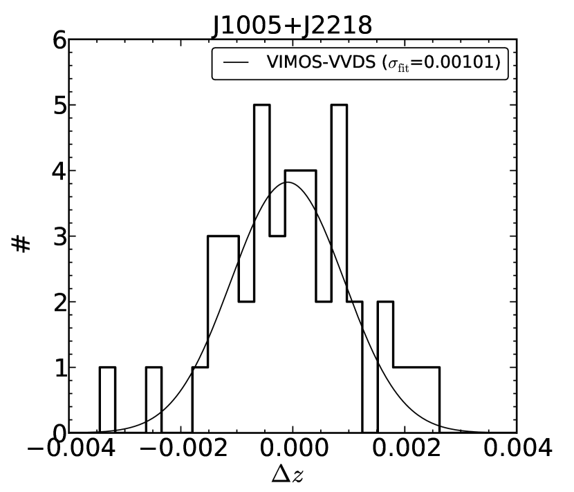
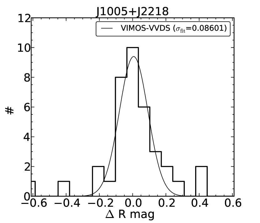
Figure 4: Difference in redshift (left panel) and $R$-band magnitude (right panel) measurements for galaxies in common between our VIMOS sample and the VVDS survey in fields J1005 and J2218. Best Gaussian fits to the histograms and standard deviation values are also shown. We see a good agreement in both redshift and magnitude measurements between the two surveys. The redshift difference distribution has a mean of $\lesssim 0.0001$ and a standard deviation of $\sigma_{\Delta z}\approx 0.001$, while the magnitude difference distribution has a mean of $\approx 0.006$ with a standard deviation of $\sigma_{\Delta{\rm R}}\approx 0.09$ magnitudes. See Section 3.5.2 for further details.

3.5.2 Consistency check between our VIMOS and VVDS sample

We performed a consistency check by comparing the redshifts and $R$-band magnitudes obtained for galaxies in common between our VIMOS sample and the VVDS survey in fields J1005 and J2218 (the only ones with such overlap). We found a good agreement in redshift measurements between the two surveys, with a mean of the distribution being $\approx 0.0003$ and a standard deviation of $\sigma_{\Delta z}\approx 0.001$. This standard deviation is consistent with the quadratic sum of the typical VVDS uncertainty ($\sim 0.0013/\sqrt{2}$) and our VIMOS one ($\sim 0.0006/\sqrt{2}$), as $\sim\sqrt{0.0006^{2}+0.0013^{2}}/\sqrt{2}\approx 0.001$. In order to place all galaxies in a single consistent frame we shifted the VVDS redshifts by $0.0003$. The left panel of Figure 4 shows the distribution of these redshift differences after applying the correction.

The right panel of Figure 4 shows the distribution of $R$-band magnitude differences. We also see a good agreement in the magnitude difference distribution (by construction, see Section 3.1), with a mean of $0.006$ and a standard deviation of $\sigma_{\Delta z}\approx 0.09$. We note that this standard deviation is greater than $\sqrt{2}\times$ the typical magnitude uncertainty as given by sextractor of $\sim 0.02$. Thus, we caution the reader that our reported $R$-band magnitude uncertainties might be underestimated by a factor of $\sim 3$.

3.6 GDDS

One of the QSOs presented in this paper (namely: J020930.7-043826) was chosen because it lies in a field already surveyed for galaxies by the GDDS survey. For our purposes we use a subsample of the whole GDDS survey selecting only galaxies in this field. We refer the reader to Abraham et al. (2004) for details on data reduction and construction of this galaxy catalog.

3.6.1 Redshift reliability

The redshift reliability for GDDS data was originally based on five subjective categories: (0) ‘educated guess’, (1) ‘very insecure’; (2) ‘reasonably secure’ (two or more spectral features); (3) ‘secure’ (two or more spectral features and continuum); (4) ‘unquestionably correct’; (8) ‘single emission line’ (assumed to be O 2); and (9) ‘single emission line’ (Abraham et al., 2004). In order to have a unified scheme we matched those GDDS labels with our previously defined VIMOS ones (see Section 3.1.5) as follows: GDDS label 4 and 3 are matched to label ‘a’ ({4,3}$\rightarrow$ {‘a’}); GDDS labels 2, 8 and 9 are matched to label ‘b’ ({2,8,9}$\rightarrow$ {‘b’}); and GDDS labels 1 and 0 are matched to label ‘c’ ({1,0}$\rightarrow$ {‘c’}).

4 IGM samples

4.1 Absorption line search

The search of absorption line systems in the continuum normalized QSO spectra was performed manually (eyeballing), based on a iterative process described as follows: (i) we first searched for all possible features (H i and metal lines) at redshift $z=0$ and $z=z_{\rm QSO}$, and labelled them accordingly. (ii) We then searched for strong H i absorption systems, from $z=z_{\rm QSO}$ until $z=0$, showing at least $2$ transitions (e.g.  and or and , and so on). This last condition allowed us to identify (strong) H i systems at redshifts greater than $z>0.477$ even for spectra without NUV coverage ($\lambda>1795$ Å). (iii) When a H i system is found, we labelled all the Lyman series transitions accordingly and looked for possible metal transitions at the same redshift. (iv) We then performed a search for ‘high-ionization’ doublets (namely: Ne 8, O 6, N 5, C 4 and Si 4), from $z=z_{\rm QSO}$ until $z=0$, independently of the presence of H i. (v) We assumed the remaining unidentified features to be H i  and repeated step (iii), unless there is evidence indicating otherwise (e.g. no detection of the transition when the spectral coverage and signal-to-noise would allow it). For all of the identified transitions we set initial guesses in number of velocity components, column densities and Doppler parameters, for a subsequent Voigt profile fitting.

This algorithm allowed us to identify the majority but not all the absorption line systems observed in our QSO spectral sample. The remaining unidentified features are typically very narrow and inconsistent with being H i (assuming a minimum temperature of the diffuse IGM of $T\sim 10^{4}$ K, implies a $b_{\rm HI}\sim 10$ ; e.g. Davé et al. 2010), so we are confident that our H i sample is fairly complete.

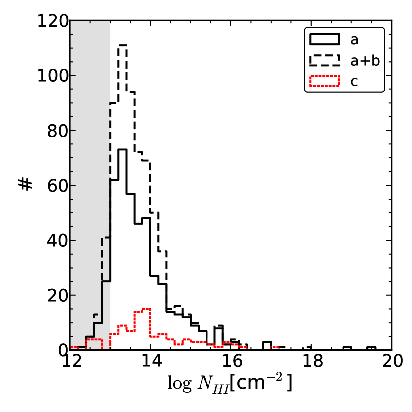
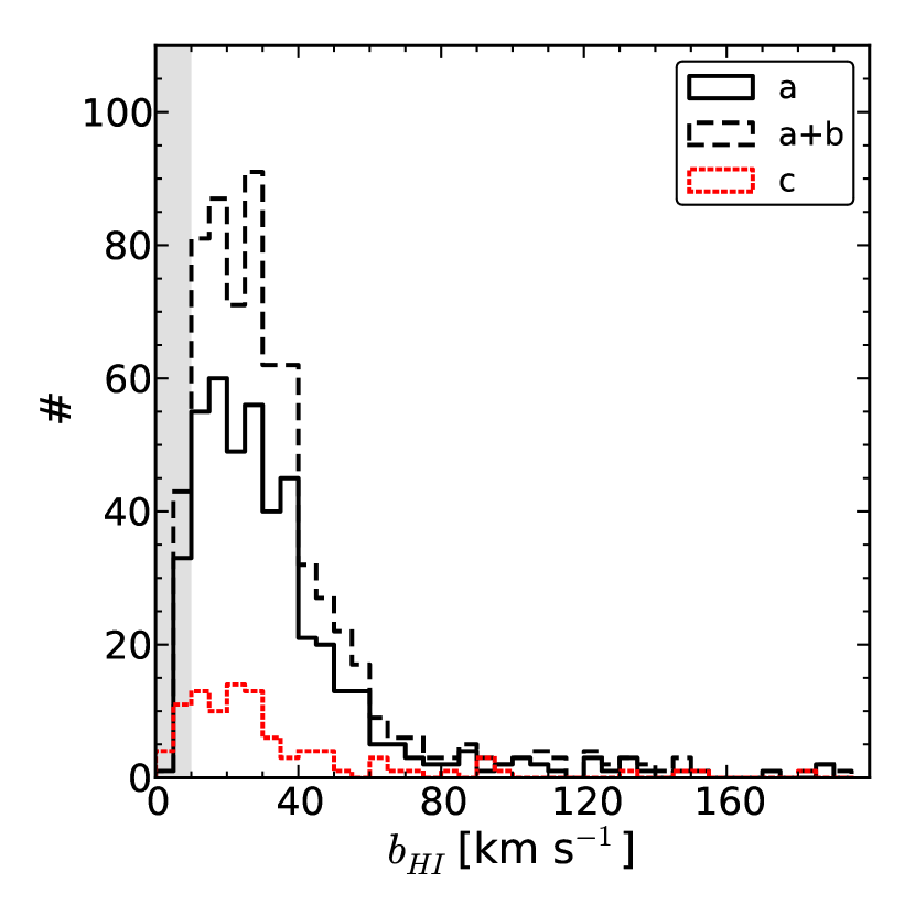
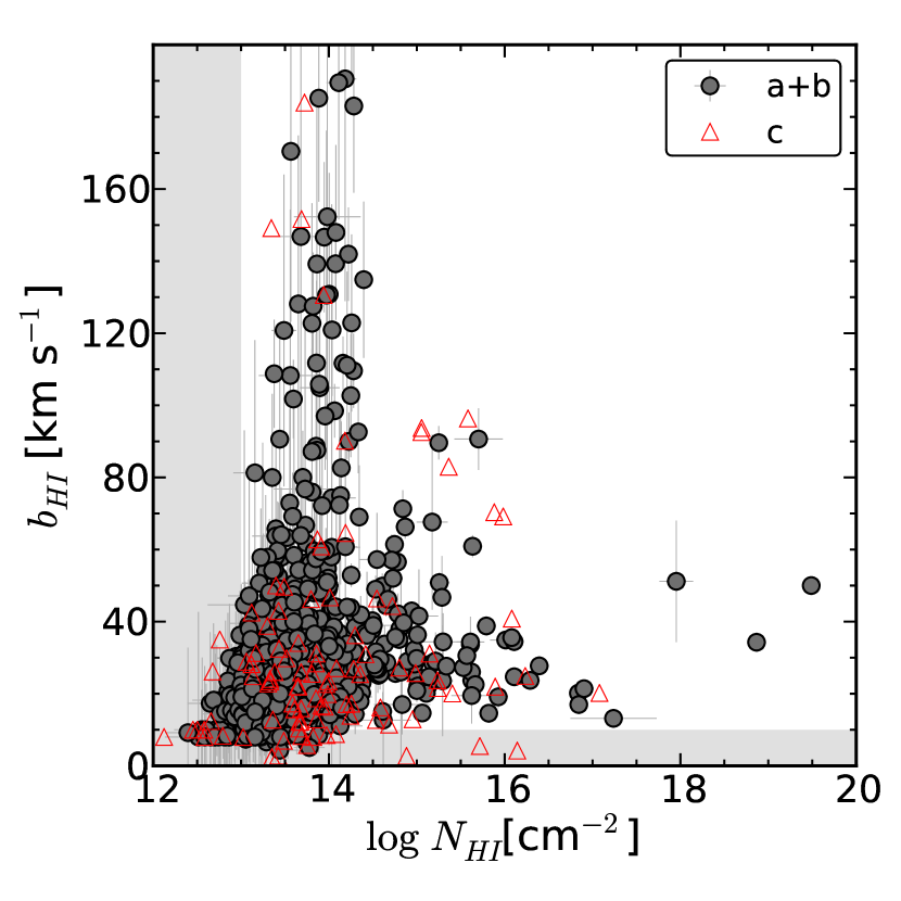
Figure 5: The first two panels show the observed H i column density ($N_{\rm HI}$; left panel) and Doppler parameter ($b_{\rm HI}$; middle panel) distributions for ‘secure’ systems (‘a’ label; black solid lines), ‘secure’ plus ‘probable’ systems (‘a$+$b’ labels; dashed black lines), and ‘uncertain’ systems (‘c’ label; dotted red lines; see Section 4.3 for definitions of these labels). The right panel shows the distribution of Doppler parameters as a function of column density for ‘secure’ plus ‘probable’ systems (‘a$+$b’ labels; grey circles), and ‘uncertain’ systems (‘c’ label; red open triangles; uncertainties not shown). Grey shaded areas show regions with low completeness levels. For further details see Section 4.5.

4.2 Voigt profile fitting

We fit Voigt profiles to the identified absorption line systems using vpfit . We accounted for the non-Gaussian COS line spread function (LSF), by interpolating between the closest COS LSF tables provided by STScI at a given wavelength. We used the guesses provided by the absorption line search (see Section 4.1) as the initial input of vpfit, and modified them when needed to reach satisfactory solutions. For intervening absorption systems we kept solutions having the least number of velocity components needed to minimize the reduced $\chi^{2}$. For fitting H i systems, we used at least two spectral regions associated to their Lyman series transitions when the spectral coverage allowed it. This means that for H i systems showing only transition, we also included their associated regions (even though they do not show evident absorption) when available. This last step provides confident upper limits to the column density of these systems. For strong H i systems we used regions associated to as many Lyman series transitions as possible, but excluding spectral regions of poor signal-to-noise ($S/N\lesssim 1$). We refer the reader to Finn et al. (2013, in prep.) for further details on the Voigt profile fitting process.

In the following we will present only results for H i systems; a catalog of metal systems will be published elsewhere.

4.3 Absorption line reliability

For each H i absorption system we assigned a reliability flag. We used a scheme based on three labels:

• Secure (‘a’): systems at redshifts that allow the detection of either  and or  and transitions in a given spectrum, whose $\log N_{\rm HI}$ values are greater than $30\times$ their uncertainties as quoted by vpfit.

• Probable (‘b’): systems at redshifts that only allow the detection of the transition in a given spectrum, whose $\log N_{\rm HI}$ values are greater than $30\times$ their uncertainties as quoted by vpfit.

• Uncertain (‘c’): systems at any redshift, whose $\log N_{\rm HI}$ values are smaller than $30\times$ their uncertainties as quoted by vpfit. Systems in this category will be excluded from the correlation analyses presented in this paper.

4.4 Consistency check of subjective steps

The whole process of finding and characterizing IGM absorption lines involves subjective steps. We checked that this fact does not affect our final results by comparing redshift, column density and Doppler parameter values for H i systems obtained independently—including the continuum fitting—by two of the authors (N.T. versus C.W.F.) in the J020930.7-043826 QSO spectrum. We found values consistent with one another at the $1\sigma$ level in $\sim 90\%$ of cases for $\log N_{\rm HI}$ and $b_{\rm HI}$, and in $100\%$ of cases for redshifts. The vast majority of discrepancies were driven by weak absorption systems close to the level of detectability, for which the differences in the continuum fitting are more important.

4.5 $N_{\rm HI}$ and $b_{\rm HI}$ distributions and completeness

In Figure 5 we show the observed H i column density ($N_{\rm HI}$; left panel) and Doppler parameter ($b_{\rm HI}$; middle panel) distributions for ‘secure’ systems (‘a’ label; black solid lines), ‘secure’ plus ‘probable’ systems (‘a$+$b’ labels; dashed black lines), and ‘uncertain’ systems (‘c’ label; dotted red lines; see Section 4.3). We see sudden decreases in the number of systems at $N_{\rm HI}\lesssim 10^{13}$  cm^-2 and $b_{\rm HI}\lesssim 10$ , which indicate the observational completeness limits of our sample and/or our selection (shown as grey shaded areas in Figure 5).

Theoretical results point out that the H i column density distribution is well described by a power law of the form $f(N_{\rm HI})\propto N_{\rm HI}^{-\beta}$ with $\beta\sim-1.7-1.8$, extending significantly below $\sim 10^{13}$  cm^-2 (e.g. Theuns, Leonard & Efstathiou, 1998; Paschos et al., 2009; Davé et al., 2010; Tepper-García et al., 2012). This has been observationally confirmed from higher signal-to-noise ratio data ($S/N\sim 20-40$) at least down to $N_{\rm HI}\sim 10^{12.3}$  cm^-2 (Williger et al., 2010). Our current $N_{\rm HI}$ completeness limit is therefore not physical, and driven by the signal-to-noise ratio of our sample. Indeed, using the results from Keeney et al. (2012), the expected minimum rest-frame equivalent width for H i lines detected in the FUV-COS—in which the majority of weak lines are detected—at the $3\sigma$ confidence level, for our typical signal-to-noise ratio ($S/N\sim 10$; see Table 2), is $\sim 40$ mÅ. This limit corresponds to $N_{\rm HI}\sim 10^{13}$  cm^-2 for a typical Doppler parameter of $b_{\rm HI}\sim 30$ , which is consistent with what we observe.

The same theoretical results point out that the H i Doppler parameter distribution for the diffuse IGM peaks at $\sim 20-40$ , with almost negligible contribution of lines with $b_{\rm HI}<10$ (Paschos et al., 2009; Davé et al., 2010; Tepper-García et al., 2012). Given that the FUV-COS data have spectral resolutions of about $\sim 16$ , these samples should include the vast majority of real H i systems at $N_{\rm HI}\gtrsim 10^{13}$  cm^-2. On the other hand, the NUV-COS and FOS data (see Table 2) have spectral resolutions of about $\sim 100$ , which introduces some unresolved lines. Unresolved blended systems also add some unphysically broad lines in all our data. This observational effect explains, in part, the tail at large $b_{\rm HI}$ (see middle panel of Figure 5). We note that very broad lines can also be explained by physical mechanisms, such as temperature, turbulence, Jeans smoothing and Hubble flow broadenings (e.g. Rutledge, 1998; Hui & Rutledge, 1999; Theuns, Schaye & Haehnelt, 2000; Davé et al., 2010; Tepper-García et al., 2012). There are a total of $58/766\sim 8\%$ of systems with $b_{\rm HI}\geq 80$ . Such a small fraction does not affect our results significantly.

We also note that the typical $b_{\rm HI}$ uncertainties are of the order of $\sim 10$ , and so scatter of a similar amount is expected in the $b_{\rm HI}$ distributions. This explains the presence of lines with $b_{\rm HI}\lesssim 10$ , all of which are consistent with $10$ within the errors. However, as we do not use the actual $b_{\rm HI}$ values in any further analysis, this uncertainty does not affect our results.

The right panel of Figure 5 shows the distribution of $b_{\rm HI}$ as a function of $\log N_{\rm HI}$ for ‘secure’ plus ‘probable’ systems (‘a$+$b’ labels; grey circles), and ‘uncertain’ systems (‘c’ label; red open triangles; uncertainties not shown). We see that there are not strong correlations between these values, apart from the presence of the upper and lower $b_{\rm HI}$ envelopes. The upper envelope is consistent with an observational effect, as higher $N_{\rm HI}$ values are required to observe lines with larger $b_{\rm HI}$, for a fixed signal-to-noise ratio (e.g. Paschos et al., 2009; Williger et al., 2010). The lower envelope is consistent with a physical effect, driven by the temperature-density relation of the diffuse IGM: H i systems with larger $N_{\rm HI}$ probe, on average, denser regions for which the temperature—a component of the $b_{\rm HI}$—is also, on average, larger (e.g. Hui & Gnedin, 1997; Theuns et al., 1999; Schaye et al., 1999; Paschos et al., 2009; Davé et al., 2010; Tepper-García et al., 2012). A proper analysis of these two effects is beyond the scope of this paper.

Table 4: Summary of the H i survey used in this paper.

	Secure	Probable	Uncertain	Total
	(‘a’)	(‘b’)	(‘c’)
Q0107-025A
H i	76	29	15	120
Strong	26	1	10	37
Weak	50	28	5	83
Q0107-025B
H i	45	6	16	67
Strong	22	1	2	25
Weak	23	5	14	42
Q0107-0232
H i	26	20	4	50
Strong	19	6	0	25
Weak	7	14	4	25
J020930.7-043826
H i	74	60	22	156
Strong	17	10	6	33
Weak	57	50	16	123
J100535.24+013445.7
H i	70	61	8	139
Strong	9	8	5	22
Weak	61	53	3	117
J102218.99+013218.8
H i	50	10	6	66
Strong	5	5	0	10
Weak	45	5	6	56
J135726.27+043541.4
H i	86	46	10	142
Strong	23	9	4	36
Weak	63	37	6	106
J221806.67+005223.6
H i	5	12	9	26
Strong	5	8	9	22
Weak	0	4	0	4
Total
H i	453	216	97	766
Strong	126	47	37	210
Weak	327	169	60	556

^a See Section 4.3 and Section 4.6 for definitions.

4.6 Column density classification

One of our goals is to test whether the cross-correlation between H i absorption systems and galaxies depends on H i column density. To do so, we split our H i sample into subcategories based on a column density limit. We define ‘strong’ systems as those with column densities $N_{\rm HI}\geq 10^{14}$  cm^-2, and ‘weak’ systems as those with $N_{\rm HI}<10^{14}$  cm^-2. The transition column density of $10^{14}$  cm^-2 is somewhat arbitrary but was chosen such that: (i) the H i–galaxy cross-correlation for ‘strong’ systems and the galaxy–galaxy auto-correlation have similar amplitudes; and (ii) the ‘strong’ systems sample is large enough to measure the cross-correlation at relatively high significance. A larger column density limit (e.g. $\sim 10^{15-16}$  cm^-2) does indeed give a stronger H i–galaxy clustering amplitude, but it also increases the noise of the measurement.

We note that there might not necessarily be a physical mechanism providing a sharp lower $N_{\rm HI}$ limit for the H i–galaxy association. However, recent theoretical results (e.g. Davé et al., 2010) suggest that there might still be a physical meaning for such a column density limit. We will discuss more on this issue in Section 8.2.5.

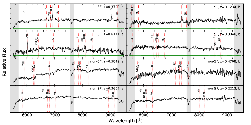
Figure 6: Examples of galaxy spectra taken with VIMOS (black lines) and their uncertainties (green lines). The left panels show spectra with ‘secure’ redshifts (‘a’ labels) while the right panels show spectra with ‘possible’ redshifts (‘b’ labels). The top four panels show examples of ‘SF’ galaxies while the bottom four panels show examples of ‘non-SF’ galaxies. Grey shaded areas show regions affected by poor sensitivity (edges) or by telluric absorption (middle) excluded from the redshift determination process. Red dotted lines show the position of some spectral features for each galaxy spectrum.

4.7 Summary

Our IGM data are composed of HST data from the COS and FOS instruments taken on $8$ different QSOs (see Tables 1 and 2). We have split our H i absorption line system sample into ‘strong’ and ‘weak’ based on a column density limit of $10^{14}$  cm^-2. Our survey is composed by a total of $\sim 669$ well identified (i.e. ‘a’ or ‘b’) H i systems with $N\gtrsim 10^{13}$  cm^-2. Table 4 shows a summary of our H i survey. Tables 9 to 20 present the survey in detail.

5 Galaxy samples

In this section we describe our galaxy samples. In the following, we will refer to our new galaxy surveys in terms of the instrument used (either VIMOS, DEIMOS and GMOS), to distinguish them from the VVDS or GDDS surveys.

5.1 Spectral type classification

One of our goals is to test whether the cross-correlation between H i absorption systems and galaxies depends on the galaxy spectral type (either absorption or emission line dominated; e.g. Chen & Mulchaey, 2009). To do so, we need to classify our galaxy sample accordingly.

We took a conservative approach by considering only two galaxy subsamples: those which have not undergone important star formation activity over their past $\sim 1$ Gyr and those which have. In terms of their spectral properties the former type has to show a strong D$4000$ break and no significant emission lines (including H$\alpha$ and [O 2]). The latter type are the complementary galaxies, i.e. those with measurable emission lines. We henceforth name these subsamples as ‘non-star-forming’ (‘non-SF’) and ‘star-forming’ (‘SF’) galaxies respectively, deliberately avoiding the misleading terminology of ‘early’ and ‘late’ types. Summarizing,

• Non-star-forming galaxies (‘non-SF’): those galaxies which show no measurable star formation activity over the past $\gtrsim 1$ Gyr (e.g. Early, Bulge, Elliptical, Red Luminous Galaxy and S0 templates).

• Star-forming galaxies (‘SF’): those galaxies which show evidence of current or recent ($\lesssim 1$ Gyr) star formation activity (e.g. Late, Sa, Sb, Sc, SBa, SBb, SBc and Starburst templates).

We note that we are not classifying galaxies on morphology, even though the template names might suggest that. Our classification is based solely on the presence or absence of spectral features associated with star-formation activity. As an example, Figure 6 shows $8$ galaxies with a variety of signal-to-noise ratios, redshifts, redshift reliabilities, and spectral classifications.

This template matching scheme was used only for our VIMOS and GMOS galaxies because in both the redshifts were determined using template matches. For the rest of our data we used different approaches, described in the following sections.

5.1.1 DEIMOS data

The DEIMOS reduction pipeline provides three weights from a principal component analysis: $w_{1}$ (‘absorption-like’), $w_{2}$ (‘emission-like’) and $w_{3}$ (‘star-like’). Thus, for DEIMOS data we use these weights to define star-forming and non-star-forming galaxies as follows: if $\max(fw_{1},w_{2})=fw_{1}$ we assigned that object to be a ‘non-SF’ galaxy; if $\max(fw_{1},w_{2})=w_{2}$ we assigned that object to be a ‘SF’ galaxy; and if $z<0.005$ we assigned that object to be a ‘star’ (this last condition takes precedence over the previous ones). We used $f=0.2$ to be conservative in the definition of ‘non-SF’ galaxies. This value also minimizes the ‘uncertain-identification rate’ in field Q0107 (see below). We did not use the information provided by $w_{3}$ because we found $7$ objects with $z>0.005$ (galaxies) showing $\max(w_{1},w_{2},w_{3})=w_{3}$, probably because of their low signal-to-noise spectra.

5.1.2 CFHT data

In the case of the CFHT survey, we did not perform a spectral type split, and so we will only use these galaxies for results involving the whole galaxy population. We note that there is a large overlap between our GMOS and the CFHT samples and that the CFHT sample is comparatively small ($61$ galaxies). Thus, this choice does not compromise our analysis.

5.1.3 VVDS data

In the case of the VVDS survey we used a color cut to split the sample into red and blue galaxies. We chose this approach because the current VVDS survey does not provide spectral classification for galaxies in the fields used in this work. We used a single color limit of $B-R=2.15$ (no ‘k-correction’ applied) to split our sample. Thus, galaxies with $B-R<2.15$ were assigned to our ‘SF’ sample, whereas those with $B-R\geq 2.15$ were assigned to our ‘non-SF’ sample. We chose this limit as it gives the same proportion of ‘non-SF’/‘SF’ galaxies as in the rest of our sample. Objects with no $B-R$ color measurement were left out of this classification, and so these will only contribute to the results involving the whole galaxy population.

Table 5: Summary of the galaxy surveys used in this paper.

	Secure	Possible	Uncertain	Undefined	Total
	(‘a’)	(‘b’)	(‘c’)	(‘n’)
Our new survey
Galaxies	1634	509	0	0	2143
‘SF’	1336	441	0	0	1777
‘non-SF’	298	68	0	0	366
Stars	451	42	0	0	493
AGN	2	20	0	0	22
Unknown	0	0	893	0	893
GGDS survey
Galaxies	41	12	0	0	53
‘SF’	32	11	0	0	43
‘non-SF’	9	1	0	0	10
Stars	1	0	0	0	1
AGN	1	0	0	0	1
Unknown	0	0	5	0	5
VVDS survey
Galaxies	9458	7903	0	0	17361
‘SF’	3766	3179	0	0	6945
‘non-SF’	789	639	0	0	1428
Stars	1	2	0	0	3
AGN	138	131	0	0	269
Unknown	0	0	8394	0	8394
CFHT survey
Galaxies	0	0	0	31	31
Total
Galaxies	11133	8424	0	31	19588
‘SF’	5134	3631	0	0	8765
‘non-SF’	1096	708	0	0	1804
Stars	453	44	0	0	497
AGN	141	151	0	0	292
Unknown	0	0	9292	0	9292

^a Only objects in field J0209.

^b Only objects in fields J1005, J1357 and J2218.

5.1.4 GDDS data

The GDDS survey provides spectral classification based on three binary digits, each one referring to ‘young’ (‘100’), ‘intermediate-age’ (‘010’) and ‘old’ (‘001’) stellar populations (Abraham et al., 2004). The GDDS spectral classification also allowed for objects dominated by one or more types, so ‘101’ could mean that the object has strong D$4000$ break and yet some strong emission lines. In order to match GDDS galaxies to our spectral classification we proceeded in the following way. Galaxies classified as ‘old’ were matched to our ‘non-SF’ sample ({‘001’}$\rightarrow$ {‘non-SF’ }); and galaxies classified as not being ‘old’ where matched to our ‘SF’ sample ({$\not=$‘001’}$\rightarrow$ {‘SF’ }).

5.1.5 Uncertainty in the spectral classification scheme

We quantified the uncertainty in this spectral classification by looking at the ‘uncertain-classification rate’, i.e. the fraction of (duplicate) galaxies that were not consistently classified as either ‘SF’ or ‘non-SF’ over the total number of (duplicate) galaxies. For fields J1005, J1022 and J2218 this uncertainly-classification rate corresponds to $11/667\sim 2\%$. None of these uncertainly-classified galaxies show redshift differences $\gtrsim 0.005$ (catastrophic). For the Q0107 field this uncertain-classification rate corresponds to $25/280\sim 9\%$. From these, $4/25$ show redshift differences $\gtrsim 0.005$, all of which are galaxies labelled as ‘b’ (‘possible’); and $19/25$ were driven by observations using different instruments. The higher uncertain-identification rate for Q0107 is therefore mostly driven by the inhomogeneity of our samples.

For fields J1005 and J2218 we also checked whether the color cut limit used to split the VVDS sample (see Section 5.1.3) gives consistency with the actual spectral classification of our VIMOS sample, for common objects observed by these two surveys. In this case, the uncertain-classification rate corresponds to $2/40\sim 5\%$, all of which were conservative in the sense that the VVDS classification (uncertain) was ‘SF’ whereas the VIMOS one (reliable) was ‘non-SF’.

5.2 Treatment of duplicates

For objects observed with different instruments and/or showing different redshift confidences, we combined their redshift information considering the following priorities:

• Redshift label priority: we gave primary priority to redshifts labelled as ‘a’, ‘b’ and ‘c’, in that order.

• Instrument priority: we gave secondary priority to redshifts measured with DEIMOS, GMOS, VIMOS and CFHT, in that order. We based this choice on spectral resolution.

We therefore chose the redshift given by the highest priority and took the average when $2$ or more observations had equivalent priorities. The spectral classification of uncertainly-classified objects (i.e., being classified as both ‘SF’ and ‘non-SF’) was set to be ‘SF’, ensuring a conservative ‘non-SF’ classification.

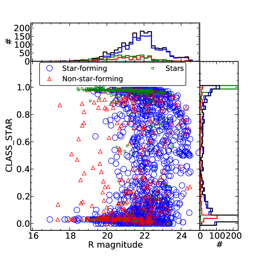
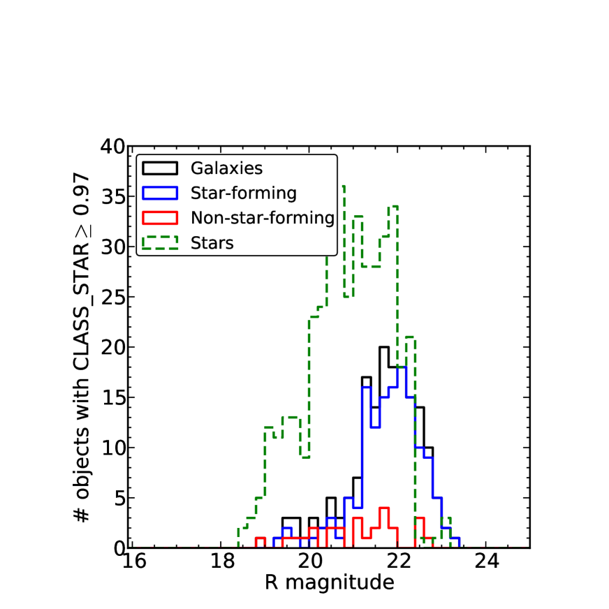
Figure 7: Left: sextractor CLASS_STAR as a function of $R$-band magnitude for objects with spectroscopic redshifts: ‘SF’ galaxies (big blue open circles), ‘non-SF’ galaxies (small red open triangles) and stars (small green squares. Histograms are shown around the main panel truncated at $230$ counts. The sudden decreases of objects at $R\sim 22$ and $R\sim 23$ are due to our target selection (see Section 3). Right: Histogram of objects with CLASS_STAR $\geq 0.97$: all galaxies (solid black), ‘SF’ galaxies (solid blue), ‘non-SF’ galaxies (solid red) and stars (dashed green). We see a significant number of unresolved galaxies at $R\gtrsim 21$ mag (see Section 5.3 for further discussion).

5.3 Star/galaxy morphological separation

Our DEIMOS observations deliberately avoided star-like (unresolved) objects, based on the CLASS_STARparameter provided by sextractor (Section 3.2). We found that this selection misses a number of faint, unresolved galaxies and so it might introduce an undesirable bias selection (see also Prochaska et al., 2011a). This motivated our subsequent VIMOS and GMOS selection, for which no morphological criteria were imposed (see Section 3.1 and Section 3.3). Here we summarize our findings regarding this issue.

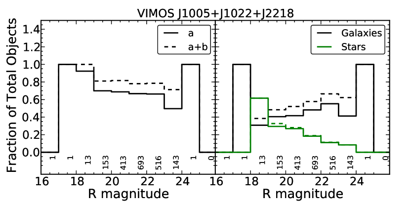
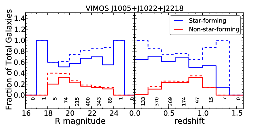
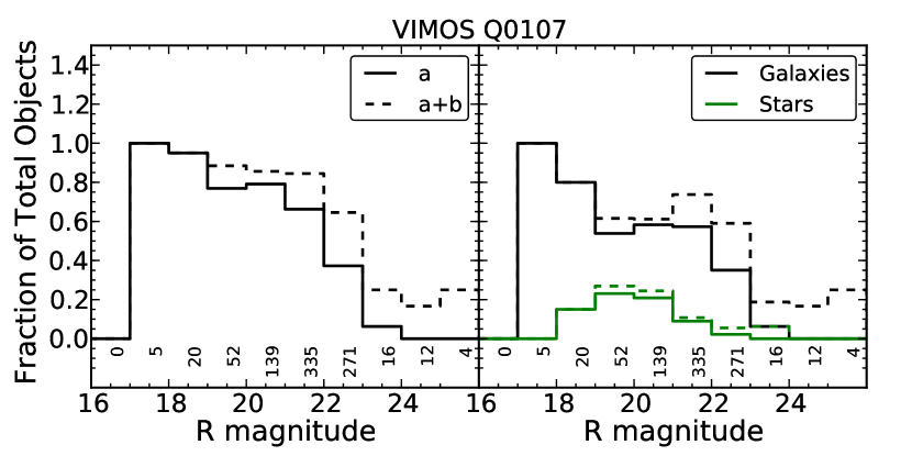
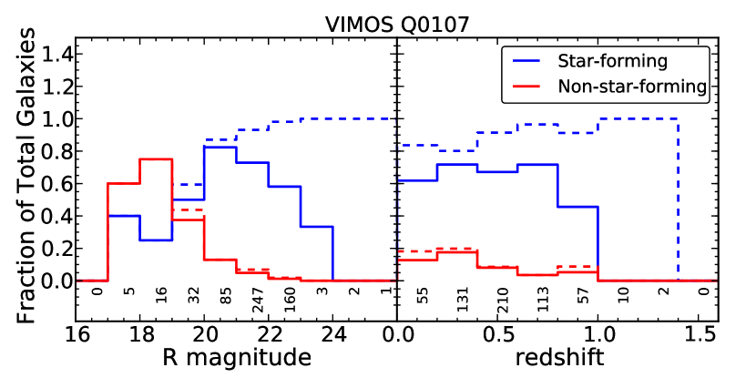
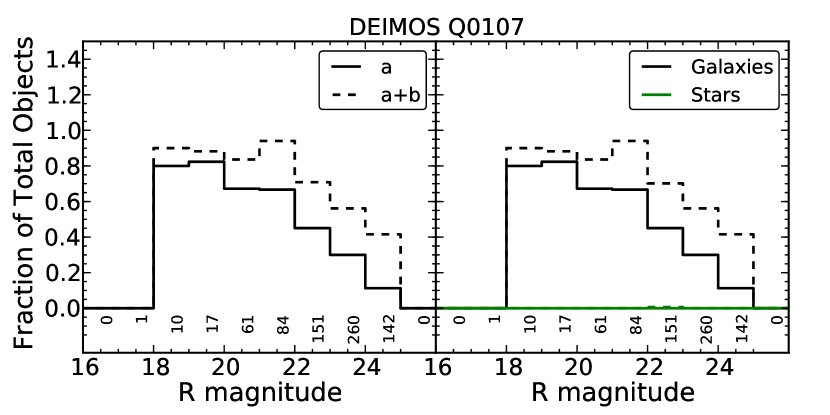
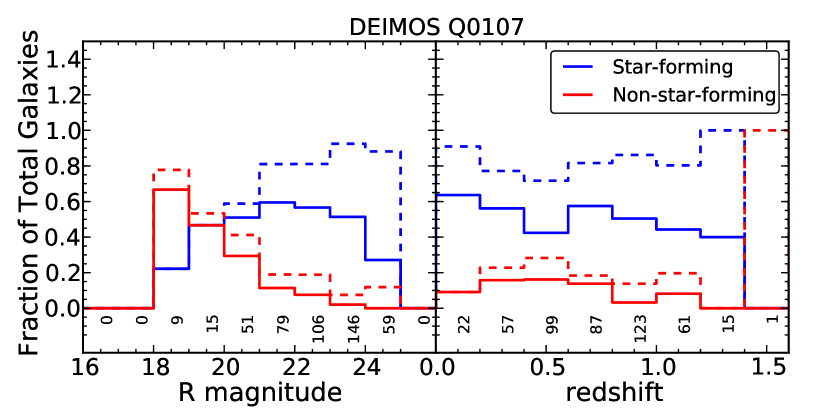
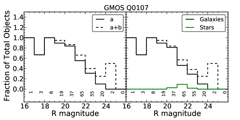
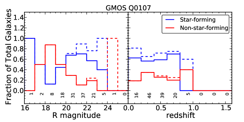
Figure 8: Success rate of assigning redshifts for our new galaxy surveys. From top to bottom: VIMOS (J1005, J1022 and J2218); VIMOS (Q0107); DEIMOS (Q0107); and GMOS (Q0107). The first and second-column panels show the fraction of targeted objects with assigned redshift and the fraction of those that were identified as galaxies (black lines) and stars (green lines), as function of apparent $R$-band magnitude, respectively. The third and fourth-column panels show the fraction of galaxies that were classified as ‘star-forming’ (blue lines) and/or ‘non-star-forming’ (red lines), as a function of $R$-band magnitude and redshift, respectively. All these fractions are shown for both objects with high (‘a’ label; solid lines) and any (‘a+b’ label; dashed lines) redshift confidence. The number of objects corresponding to a fraction of $1$ (total) are labeled at the bottom of each bin. See Section 5.4 for further discussion.

The left panel of Figure 7 shows CLASS_STAR values as a function of $R$-band magnitude for objects with spectroscopic redshifts: ‘SF’ galaxies (big blue open circles), ‘non-SF’ galaxies (small red open triangles) and stars (small green squares). The sudden decrease of objects at $R\sim 22.5$, $R\sim 23.5$ and $R\sim 24.5$ magnitudes are due to our target selection (see Section 3). The fraction of ‘non-SF’ with respect to ‘SF’ galaxies is higher at brighter magnitudes (see Section 5.4). We see a bimodal distribution of objects having CLASS_STAR $\sim 0$ (resolved) and CLASS_STAR $\sim 1$ (unresolved). The vast majority of resolved objects are galaxies but some stars also fall in this category due to the non-uniform point spread function (PSF) that varies across the imaging field of view. On the other hand, the vast majority of bright unresolved objects are stars, but a significant fraction of faint ones are galaxies. The right panel of Figure 7 shows a histogram of objects with CLASS_STAR $\geq 0.97$ as a function of $R$-band magnitude. Such objects are typically excluded from galaxy spectroscopic surveys. We find unresolved galaxies over a wide range of magnitudes, but more importantly at $R\gtrsim 21$. At $R\gtrsim 22$ unresolved galaxies dominate over stars, and so a CLASS_STAR $<0.97$ criteria indeed introduces an undesirable selection bias. Even at magnitudes brighter than $R\sim 21$, where the fraction of unresolved galaxies is small, this morphological bias is still undesirable for galaxy-absorber direct association studies. In our survey, $2$($7$) out of $33$($82$) $R\leq 21$ ($R\leq 24$) unresolved galaxies lie at $\leq 300$  kpc (physical) from a QSO LOS which might have been left out based on a morphological selection. As mentioned, our DEIMOS survey is indeed affected by this selection effect, but our VIMOS and GMOS surveys are not, which allowed us to overcome this potential problem in all our fields, including Q0107.

Neither the VVDS nor the GDDS data are affected in this way. The VVDS survey targeted objects based only on magnitude limits, while the GDDS survey used photometric redshifts to avoid low-$z$ galaxies, with no morphological criteria imposed.

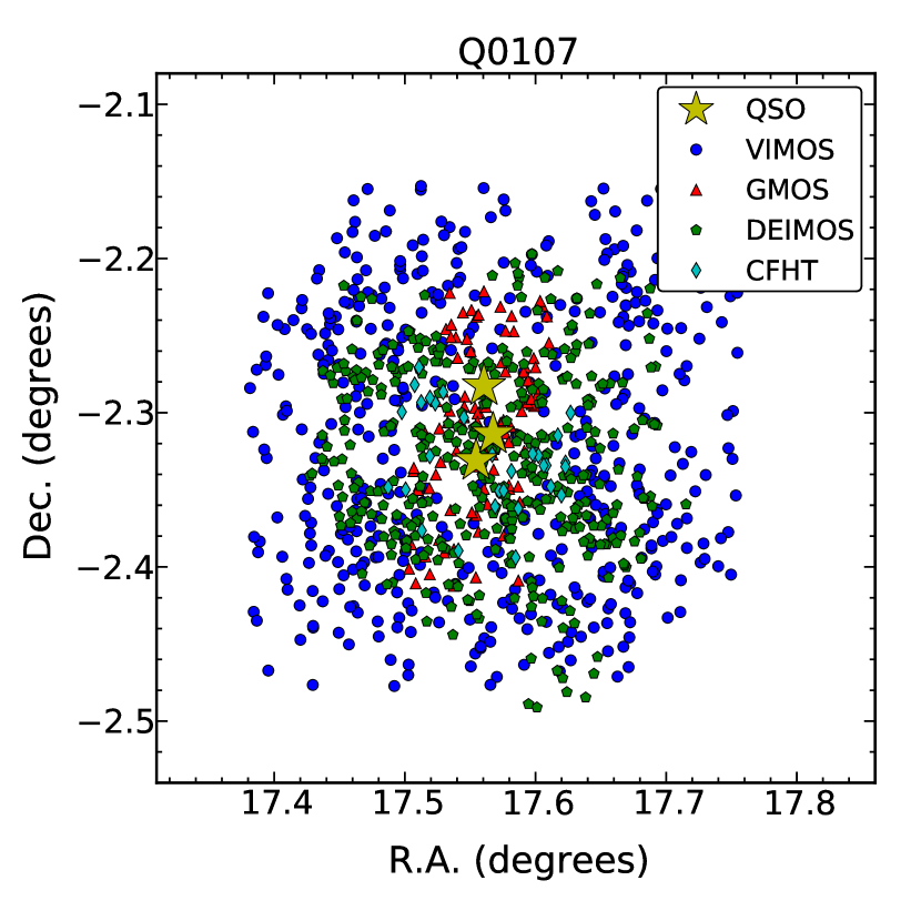
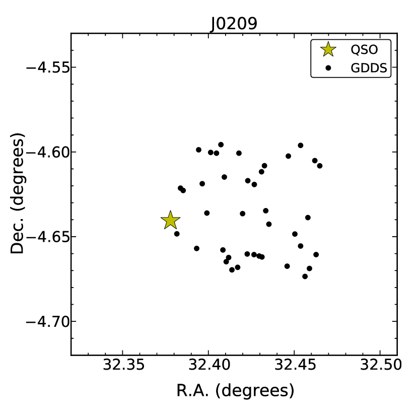
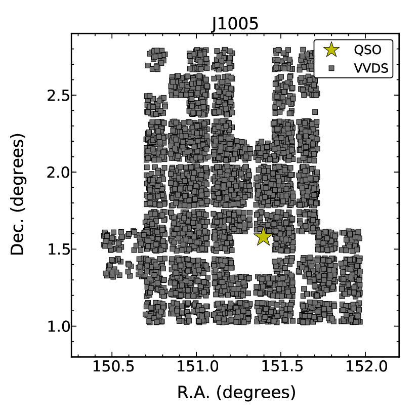
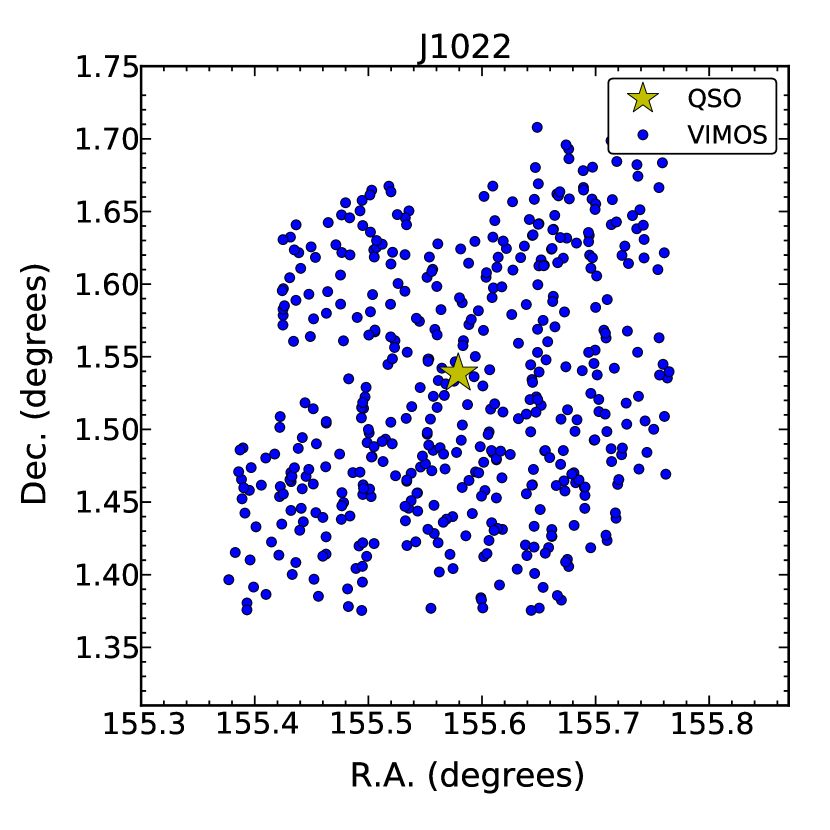
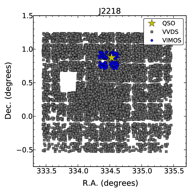
Figure 9: Distribution on the sky of galaxies and background QSOs (yellow stars) for each field. Blue circles, red triangles and green pentagons correspond to our new VIMOS, GMOS and DEIMOS galaxies respectively; while black circles, grey squares and cyan diamonds correspond to GDDS, VVDS and CFHT MOS galaxies respectively.

5.4 Completeness

The completeness of a survey is defined as the fraction of detected objects with respect to the total number of objects that could be observed given the selection criteria. In the case of our galaxy survey the completeness can be decomposed in: (i) the fraction of objects with successful redshift determination with respect to the total number of targeted objects; (ii) the fraction of targeted objects with respect to the total number of objects detected by sextractor; and (iii) the fraction of objects detected by sextractor with respect to the total number of objects that could be observed. In the following we will focus only on the first of these terms for our new galaxy data. For the completeness of VVDS, GDDS and CFHT surveys we refer the reader to Le Fèvre et al. (2005), Le Fevre et al. (2013), Abraham et al. (2004) and Morris & Jannuzi (2006).

In Figure 8 we show the success rate of assigning redshifts as a function of $R$-band apparent magnitude, for all objects (first-column panels) and for galaxies and/or stars (second-column panels). We present them separately for each of our new galaxy surveys because of their different selection functions. From top to bottom: VIMOS (J1005, J1022 and J2218), VIMOS (Q0107), DEIMOS (Q0107), and GMOS (Q0107). All of these fractions are computed for objects whose redshifts have been measured at high (label ‘a’, solid lines) and/or any confidence (label ‘a+b’, dashed lines). We see that our surveys have a $\sim 70-90\%$ success rate for objects with $R\lesssim 22$ magnitudes, and a $\lesssim 40\%$ success rate for objects with $22\lesssim R\lesssim 24$, except for our VIMOS survey of fields J1005, J1022 and J2218, which shows a $\sim 70-90\%$ success rate even for faint objects. As mentioned in Section 3 our VIMOS, GMOS and DEIMOS surveys were limited at $R=23-23.5$, $R=24$, $R=24.5$ respectively, and so the small contribution of objects fainter than those limits correspond to untargeted objects that happened to lie within the slits. These objects correspond to a very small fraction of the total, and so we left them in. The higher success rate for brighter objects is expected given the higher signal-to-noise ratio of those spectra. For objects brighter than $R\sim 22$ magnitudes, the fraction of identified galaxies is $\gtrsim 50\%$, and the fraction of identified stars varies: from $\sim 0\%$ in our DEIMOS survey (by construction; see Section 3.2), $\lesssim 10\%$ in our GMOS survey, to $\sim 20-10\%$ in our VIMOS surveys. The fraction of identified galaxies and stars at fainter magnitudes is $\lesssim 50\%$ and $\lesssim 10\%$ respectively.

Figure 8 also shows how the galaxy completeness depends on our galaxy spectral type classification (see Section 5.1). The third and fourth-column panels show the fraction of galaxies classified as ‘SF’ (blue lines) and ‘non-SF’ (red lines) over the total number of galaxies as a function of $R$-band magnitude and redshift respectively. Excluding magnitude bins with $<10$ galaxies, we see that the fraction of ‘non-SF’ galaxies decreases with $R$-band apparent luminosity, consistent with the higher signal-to-noise ratio spectra for the brighter objects. The fraction of ‘SF’ galaxies shows a flatter behavior because the redshift determination depends more on the signal-to-noise of the emission lines than the signal-to-noise of the continuum. The fraction of ‘non-SF’ galaxies dominates over ‘SF’ ones at $R\lesssim 19$ (see also left panel Figure 7), with a contribution of $\sim 50-70\%$, although these bins have typically $<20$ objects. At fainter magnitudes ($R\gtrsim 20$), ‘SF’ galaxies dominate over ‘non-SF’ ones with a contribution of $\sim 60-90\%$. Despite these magnitude trends, we see that our galaxy sample is dominated by the ‘SF’ type over the whole redshift range (except for the one galaxy observed at $z>1.4$ in the DEIMOS survey), as might have been expected from our conservative spectral classification (Section 5.1). ‘SF’ (‘non-SF’) galaxies account for $\sim 60-80\%$ ($\sim 20-30\%$) of the total galaxy fraction at $z\lesssim 1$, with a mild decrease (increase) with redshift. This redshift trend is most apparent in our VIMOS survey of fields J1005, J1022 and J2218, which we explain as follows. The D$4000$ Å break becomes visible at $5500$ Å for redshifts $\sim 0.4$ and moves towards wavelength ranges of higher spectral quality ($\sim 6000-7500$ Å) at $z\sim 0.7-0.9$. Simultaneously, H$\alpha$ and [O 3] emission lines are shifted towards poor quality spectral ranges ($\gtrsim 8000$ Å; due to the presence of sky emission lines) at $z\sim 0.2$ and $z\sim 0.6$, and are out of range at $z\gtrsim 0.4$ and $z\gtrsim 0.8$ respectively. At $z\gtrsim 1$ the only emission line available is [O 2] which explains the rise in the fraction of low redshift confidence (‘b’ labels) ‘SF’ galaxies.

5.5 Summary

Our galaxy data is composed of a heterogeneous sample obtained from $4$ different instruments (see Table 3), taken around $8$ different QSO LOS in $6$ different fields (see Figure 9 and Table 1). For fields with observations from more than one instrument, we have made sure that the redshift frames are all consistent. We have also split the galaxies into ‘star-forming’ (‘SF’) and ‘non-star-forming’ (‘non-SF’), based on either spectral type (for those lying close to the QSO LOS, i.e., VIMOS, DEIMOS, GMOS and GDDS samples) or color (VVDS sample). Table 5 shows a summary of our galaxy survey. Tables 21 to 24 present our new galaxy survey in detail. We refer the reader to Le Fèvre et al. (2005), Le Fevre et al. (2013), Abraham et al. (2004) and Morris & Jannuzi (2006) for retrieving the VVDS, GDDS and CFHT data respectively.

Our final dataset comprises $19588$ ($11133$) galaxies with good (excellent) spectroscopic redshifts at $z\lesssim 1$ around QSO LOS with $669$ ($453$) good (excellent) H i absorption line systems. This is currently the largest sample suitable for a statistical analysis on the IGM–galaxy connection to date.

6 Correlation analysis

The main goal of this paper is to address the connection between the IGM traced by H i absorption systems and galaxies in a statistical manner. To do so, we focus on a two-point correlation analysis rather than attempting to associate individual H i systems with individual galaxies.

The two-point correlation function, $\xi(r)$, is defined as the probability excess of finding a pair of objects at a distance $r$ with respect to the expectation from a randomly distributed sample. Combining the results from the H i–galaxy cross-correlation with those from the H i–H i and galaxy–galaxy auto-correlations for different subsamples of H i systems and galaxies, we aim to get further insights into the relationship between the IGM and galaxies.

Figure 10: Total number of cross-pairs between H i absorption systems and galaxies as a function of separations along ($r_{\parallel}$; $y$-axes) and transverse to the line-of-sight ($r_{\perp}$; $x$-axes). From left to right: $D_{\rm a}D_{\rm g}$ is the number of observed ‘data-data’ absorber–galaxy pairs; $R_{\rm a}R_{\rm g}$ is the number of ‘random-random’ absorber–galaxy pairs; and $D_{\rm a}R_{\rm a}$ and $R_{\rm a}D_{\rm g}$ are the number of ‘data-random’ and ‘random-data’ absorber–galaxy pairs respectively. We used an arbitrary binning of $0.5$  Mpc with a Gaussian smoothing of standard deviation of $0.5$  Mpc along both directions.

6.1 Two-dimensional correlation measurements

In order to measure these spatial correlation functions we converted all H i systems and galaxy positions given in (RA, DEC, $z$) coordinates into a Cartesian co-moving system $(X,Y,Z)$. We first calculated the radial co-moving distance to an object at redshift $z$ as,

$$R(z)=\frac{c}{H_{0}}\int_{0}^{z}\!\frac{1}{\sqrt{\Omega_{\rm m}(1+z^{\prime})^{3}+\Omega_{\Lambda}}}\,{\rm d}z^{\prime}\ \rm{.}$$ (2)

where $c$ is the speed of light, $H_{0}$ is the Hubble constant and, $\Omega_{\rm m}$ and $\Omega_{\rm\Lambda}$ are the mass and ‘dark energy’ density parameters, respectively. Let (RA₀, DEC₀) be the central coordinates of a given independent field. We then transformed (RA,DEC,$z$) to $(X,Y,Z)$ as follows:

$$\begin{split}X&\equiv R(z)\cos{(\Delta\delta)}\cos{(\Delta\alpha)}\\ Y&\equiv R(z)\cos{(\Delta\delta)}\sin{(\Delta\alpha)}\\ Z&\equiv R(z)\sin{(\Delta\delta)}\ \rm{,}\end{split}$$ (3)

where $\Delta\delta\equiv({\rm DEC}-{\rm DEC}_{0})$ and $\Delta\alpha\equiv({\rm RA}-{\rm RA}_{0})\cos({\rm DEC}_{0})$, both in radians. Note that all our fields are far away from the poles and each of them has small angular coverage (‘pencil beam’ surveys), making this transformation accurate. For fields with only one QSO we chose $({\rm RA}_{0},{\rm DEC}_{0})=({\rm RA}_{\rm QSO},{\rm DEC}_{\rm QSO})$, while for the triple QSO field we took the average position as the central one.

Given that peculiar velocities add an extra component to the redshifts (in addition to cosmological expansion), our $(X,Y,Z)$ will be affected differently, producing distortions even for actually true isotropic signals. This is because the $X$ coordinate is parallel to the LOS, while the $Y$ and $Z$ coordinates are perpendicular to it. Let $R(z)$ be the radial co-moving distance at redshift $z$ (Equation 2) and $\Delta\theta$ a small ($\ll 1$) angular separation in radians. The transverse co-moving separation can be then approximated by $\approx R(z)\Delta\theta$, implying that our $X$ coordinate will be affected a factor of $\approx 1/\Delta\theta$ times that of the $Y$ and $Z$ coordinates for a fixed redshift difference. As an example, a redshift difference of $\Delta z=0.0007$ at $z=0.5$ ($\approx 140$ ) will roughly correspond to a radial co-moving difference of $\approx 2$  Mpc, while only to a $\lesssim 0.02$  Mpc difference in the transverse direction for co-moving separations $\lesssim 20$  Mpc. We therefore measured the auto- and cross-correlations both along and transverse to the LOS, $\xi(r_{\perp},r_{\parallel})$, independently. In terms of our Cartesian coordinates we have that $r_{\parallel,ij}\equiv|X_{i}-X_{j}|$ and $r_{\perp,ij}\equiv\sqrt{|Y_{i}-Y_{j}|^{2}+|Z_{i}-Z_{j}|^{2}}$, are the along the LOS and transverse to the LOS distances between two objects at positions $(X_{i},Y_{i},Z_{i})$ and $(X_{j},Y_{j},Z_{j})$ respectively. Deviations from an isotropic signal in our $(r_{\perp},r_{\parallel})$ coordinates can then be attributed to redshift uncertainties and peculiar velocities, including large scale structure (LSS) bulk motions between the objects in the sample.

We used the Landy & Szalay (1993) estimator to calculate the galaxy–galaxy auto-correlation as,

$$\xi^{\rm LS}_{\rm gg}(r_{\perp},r_{\parallel})=\frac{D_{\rm g}D_{\rm g}/n_{\rm gg}^{\rm DD}-2D_{\rm g}R_{\rm g}/n_{\rm gg}^{\rm DR}}{R_{\rm g}R_{\rm g}/n_{\rm gg}^{\rm RR}}+1\ \rm{,}$$ (4)

where $D_{\rm g}D_{\rm g}$ is the number of observed ‘data-data’ galaxy–galaxy pairs, $R_{\rm g}R_{\rm g}$ is the number of ‘random-random’ galaxy–galaxy pairs and $D_{\rm g}R_{\rm g}$ is the number of ‘data-random’ galaxy–galaxy pairs, all of which are measured at the given $(r_{\perp},r_{\parallel})$ scales; and $n_{\rm gg}^{\rm DD}$, $n_{\rm gg}^{\rm DR}$ and $n_{\rm gg}^{\rm RR}$ are the normalization factors for each respective pair count. Let $N_{\rm gal}^{\rm real}$ and $N_{\rm gal}^{\rm rand}\equiv\alpha_{\rm gal}N_{\rm gal}^{\rm real}$ be the total number of real and random galaxies respectively, then

$$\begin{split}n^{\rm DD}_{\rm gg}&=N_{\rm gal}^{\rm real}(N_{\rm gal}^{\rm real}-1)/2\\ n^{\rm DR}_{\rm gg}&=\alpha_{\rm gal}(N_{\rm gal}^{\rm real})^{2}\\ n^{\rm RR}_{\rm gg}&=\alpha_{\rm gal}N_{\rm gal}^{\rm real}(\alpha_{\rm gal}N_{\rm gal}^{\rm real}-1)/2\rm{.}\end{split}$$ (5)

The H i–H i auto-correlation, $\xi^{\rm LS}_{\rm aa}$, was calculated in a similar fashion as $\xi^{\rm LS}_{\rm gg}$,

$$\xi^{\rm LS}_{\rm aa}(r_{\perp},r_{\parallel})=\frac{D_{\rm a}D_{\rm a}/n_{\rm aa}^{\rm DD}-2D_{\rm a}R_{\rm a}/n_{\rm aa}^{\rm DR}}{R_{\rm a}R_{\rm a}/n_{\rm aa}^{\rm RR}}+1\ \rm{,}$$ (6)

where $D_{\rm a}D_{\rm a}$ is the number of observed ‘data-data’ absorber-absorber pairs, $R_{\rm a}R_{\rm a}$ is the number of ‘random-random’ absorber-absorber pairs and $D_{\rm a}R_{\rm a}$ is the number of ‘data-random’ absorber-absorber pairs, all of which measured at the given $(r_{\perp},r_{\parallel})$ scales; and $n_{\rm aa}^{\rm DD}$, $n_{\rm aa}^{\rm DR}$ and $n_{\rm aa}^{\rm RR}$ are the normalization factors for each respective pair count. Let $N_{\rm abs}^{\rm real}$ and $N_{\rm abs}^{\rm rand}\equiv\alpha_{\rm abs}N_{\rm abs}^{\rm real}$ be the total number of real and random H i systems respectively, then

$$\begin{split}n^{\rm DD}_{\rm aa}&=N_{\rm abs}^{\rm real}(N_{\rm abs}^{\rm real}-1)/2\\ n^{\rm DR}_{\rm aa}&=\alpha_{\rm abs}(N_{\rm abs}^{\rm real})^{2}\\ n^{\rm RR}_{\rm aa}&=\alpha_{\rm abs}N_{\rm abs}^{\rm real}(\alpha_{\rm abs}N_{\rm abs}^{\rm real}-1)/2\rm{.}\end{split}$$ (7)

The H i–galaxy cross-correlation, $\xi^{\rm LS}_{\rm ag}$, was calculated using a generalized version of the Landy & Szalay (1993) estimator,

$$\xi^{\rm LS}_{\rm ag}(r_{\perp},r_{\parallel})=\frac{D_{\rm a}D_{\rm g}/n_{\rm ag}^{\rm DD}-D_{\rm a}R_{\rm g}/n_{\rm ag}^{\rm DR}-R_{\rm a}D_{\rm g}/n_{\rm ag}^{\rm RD}}{R_{\rm a}R_{\rm g}/n_{\rm ag}^{\rm RR}}+1$$ (8)

(e.g. Adelberger et al., 2003), where $D_{\rm a}D_{\rm g}$ is the number of observed ‘data-data’ absorber–galaxy pairs, $R_{\rm a}R_{\rm g}$ is the number of ‘random-random’ absorber–galaxy pairs, and $D_{\rm a}R_{\rm a}$ and $R_{\rm a}D_{\rm g}$ are the number of ‘data-random’ and ‘random-data’ absorber–galaxy pairs respectively, all of which are measured at the given $(r_{\perp},r_{\parallel})$ scales. Following previous conventions the normalization factors in this case are,

$$\begin{split}n^{\rm DD}_{\rm ag}&=N_{\rm abs}^{\rm real}N_{\rm gal}^{\rm real}\\ n^{\rm DR}_{\rm ag}&=\alpha_{\rm gal}N_{\rm abs}^{\rm real}N_{\rm gal}^{\rm real}\\ n^{\rm RD}_{\rm ag}&=\alpha_{\rm abs}N_{\rm abs}^{\rm real}N_{\rm gal}^{\rm real}\\ n^{\rm RR}_{\rm ag}&=\alpha_{\rm gal}\alpha_{\rm abs}N_{\rm abs}^{\rm real}N_{\rm gal}^{\rm real}\ \rm{.}\end{split}$$ (9)

This approach makes the random samples a crucial component of the analysis. A detailed description of the random generator algorithms is presented in Section 6.2.

Landy & Szalay (1993) showed that $\xi^{\rm LS}$ minimizes the observed variance and so is preferable over other proposed estimators (e.g. Sharp, 1979; Hewett, 1982; Davis & Peebles, 1983; Hamilton, 1993). Given the limited nature of any survey, all estimators are biased towards lower correlation amplitudes. This is because the mean densities of our two populations are estimated from the survey itself. In order for us to measure a positive correlation on a certain scale, the measured $\xi$ needs to be negative at another. This leads to an observed correlation amplitude which is lower than the underlying real one, $\xi^{\rm real}$, assumed to be positive. This is a well known bias commonly referred to as the ‘integral constraint’. Landy & Szalay (1993) showed that $\xi^{\rm LS}$ and $\xi^{\rm real}$ are related as

$$1+\xi^{\rm LS}=\frac{\ \ 1+\xi^{\rm real}}{1+\xi_{V}}\ \rm{,}$$ (10)

where $\xi_{V}$ is the ‘integral constraint’ (scalar) defined as

$$\xi_{V}\equiv\int_{V}\,G(r)\xi^{\rm real}(r)\,{\rm d}^{2}V\ \rm{.}$$ (11)

Here $G(r)$ is a normalized geometric window function (positive) which gives the probability of having two volume elements separated by a distance $r$ in the survey. In the case of our auto- and cross-correlations, $G$ is given by $G_{\rm gg}\approx R_{\rm g}R_{\rm g}/n^{\rm gg}_{\rm RR}$, $G_{\rm aa}\approx R_{\rm a}R_{\rm a}/n^{\rm aa}_{\rm RR}$ and $G_{\rm ag}\approx R_{\rm a}R_{\rm g}/n^{\rm ag}_{\rm RR}$. Although we cannot know a priori the amplitude of $\xi^{\rm real}$, we made a small correction using

$$\xi=(1+\tilde{\xi}_{V})(1+\xi^{\rm LS})-1\ \rm{,}$$ (12)

where $\tilde{\xi}_{V}\equiv\int_{V}\,G(r)\xi^{\rm LS}(r)\,{\rm d}^{2}V$, which still helps because of the discrete nature of all our cross-pair counts (including the randoms).

The computation of $\xi_{\rm gg}^{\rm LS}$, $\xi_{\rm aa}^{\rm LS}$ and $\xi_{\rm ag}^{\rm LS}$ was performed after summing all the cross-pairs from our $N_{\rm f}=6$ independent fields,

$$D_{\rm g}D_{\rm g}(r_{\perp},r_{\parallel})=\sum\limits_{i}^{N_{\rm f}}D_{\rm g}D_{\rm g}(r_{\perp},r_{\parallel})_{i}\ \rm{,}$$ (13)

where $(D_{\rm g}D_{\rm g})_{i}$ is the number of ‘data-data’ galaxy–galaxy pairs in the $i$-th field, and so on for the rest of the cross-pair counts. In contrast to measuring $\xi^{\rm LS}$ for each independent field and then taking a weighted average, our adopted approach reduces the ‘shot noise’.

Another way to reduce the ‘shot noise’ is by using large bin sizes for counting the cross-pairs, but this will limit the spatial resolution of our $\xi$ measurements. Therefore, we have chosen to compute the cross-pairs at scales $r_{\perp}<10$  Mpc using a linear grid of $0.5$  Mpc in both $(r_{\perp},r_{\parallel})$ coordinates and apply a Gaussian filter of $0.5$  Mpc standard deviation (in both directions) to smooth the final counts distribution obtained from Equation 13 before applying Equations 4, 6 and 8. We treated the edges of the grid as if they were mirrors for the smoothing. As an example, Figure 10 shows the number of cross-pairs between H i absorption systems and galaxies for our ‘Full Sample’ (defined in Section 7) using our adopted binning and smoothing.

An isotropic smoothing is desirable to avoid introducing artificial distortions, especially at the smallest scales. The use of a smoothing filter is justified by assuming that the underlying matter distribution that gives rise to H i absorption systems and galaxies (and hence to the data-data cross-pairs) is also smooth. Our approach offers a compromise between reducing the ‘shot noise’ while keeping a relatively small bin size. We caution though, that if the geometry of H i clouds does contain sharp edges at scales smaller than our adopted binning or smoothing length, then we would not be able to detect such a feature.

6.2 Random samples

One of the crucial steps for a correlation analysis is the construction of the random samples. In order to cancel out any possible bias we preserved the sensitivity function of the real survey in our random samples. A detailed description of the random generator algorithms for H i absorption systems and galaxies is presented in the following sections.

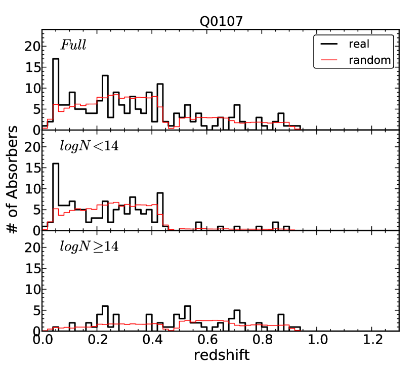
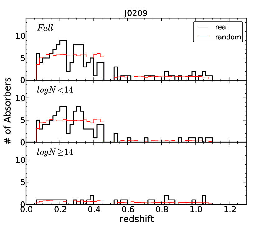
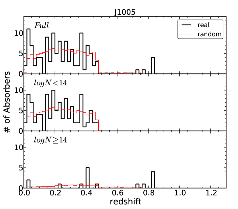
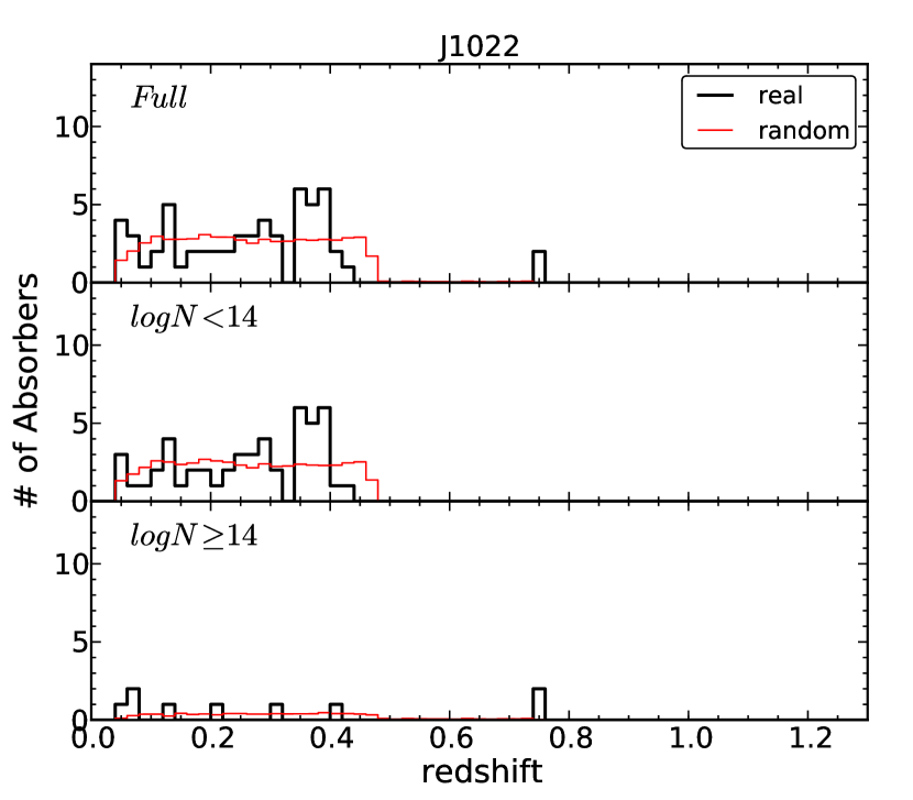
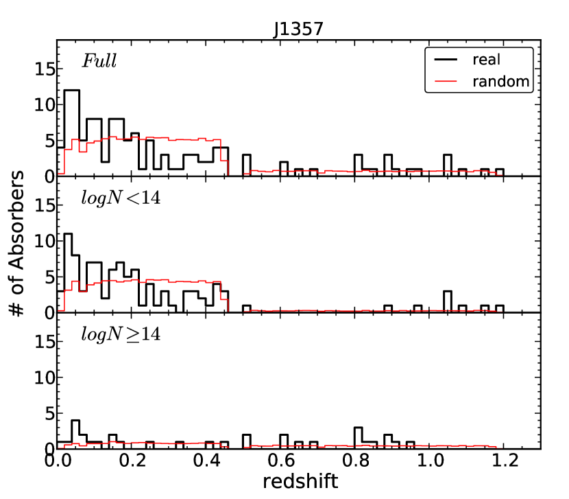
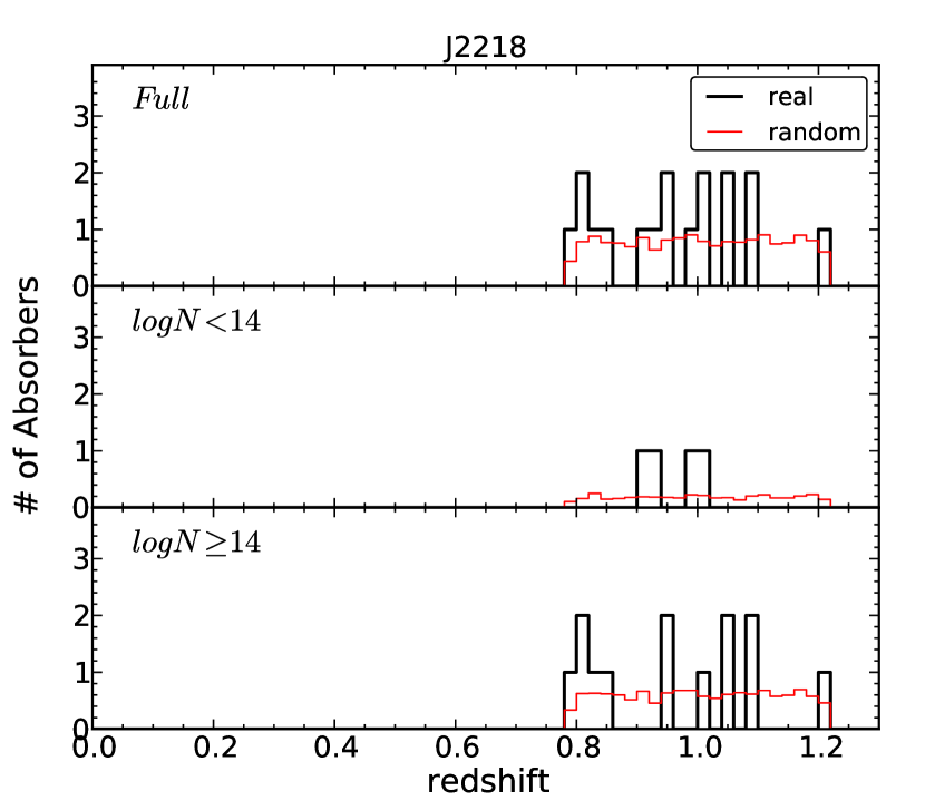
Figure 11: Histograms of the H i absorption systems redshift distribution for our different fields ($0.02$ binning). The black thick solid lines correspond to the real distributions whereas the red thin solid lines correspond to the normalized random expectation drawn from samples of $200\times$ the real sample sizes. A full description of the random generator algorithm can be found in Section 6.2.1. Top panels show the full H i samples while the middle and bottom panels show subsamples based on $N_{\rm HI}$ cuts.

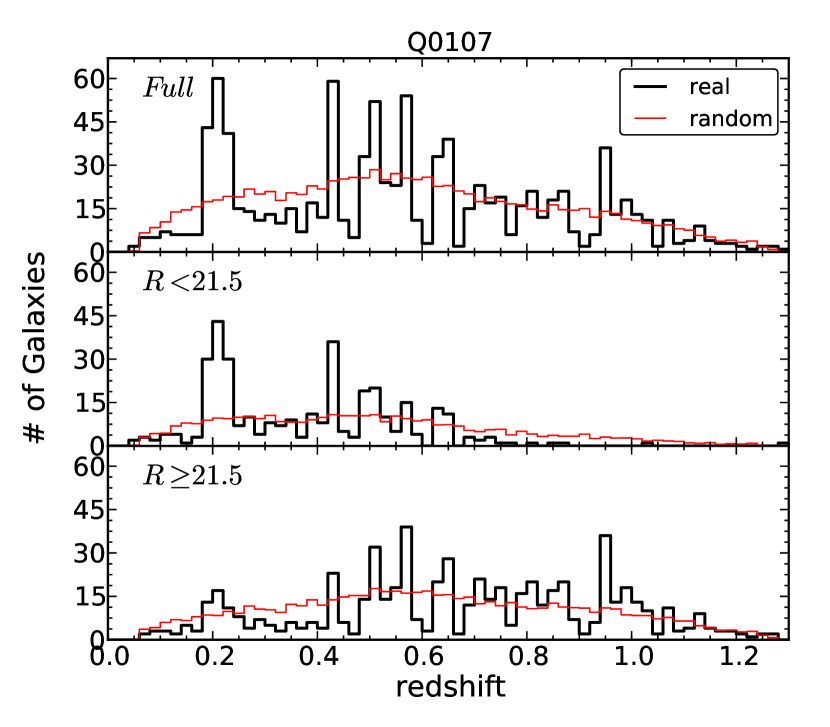
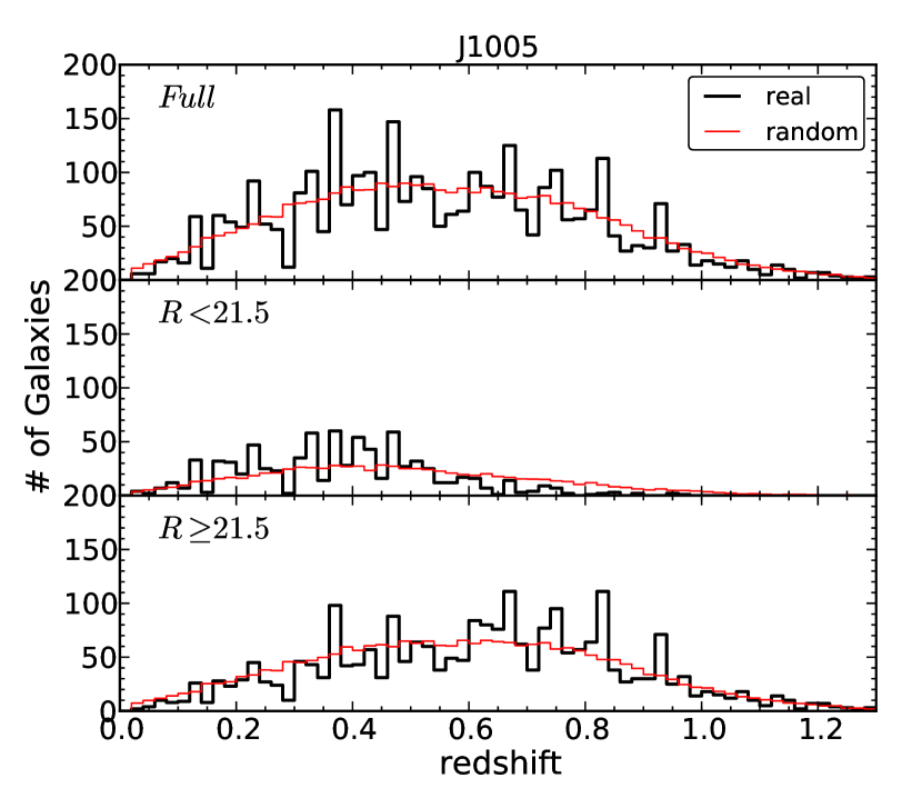
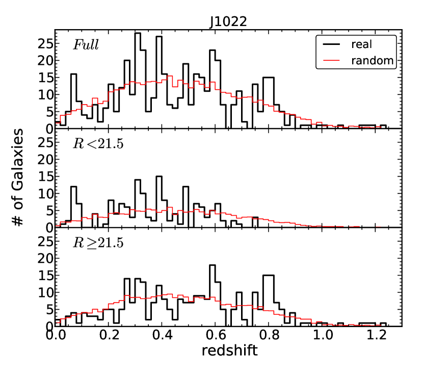
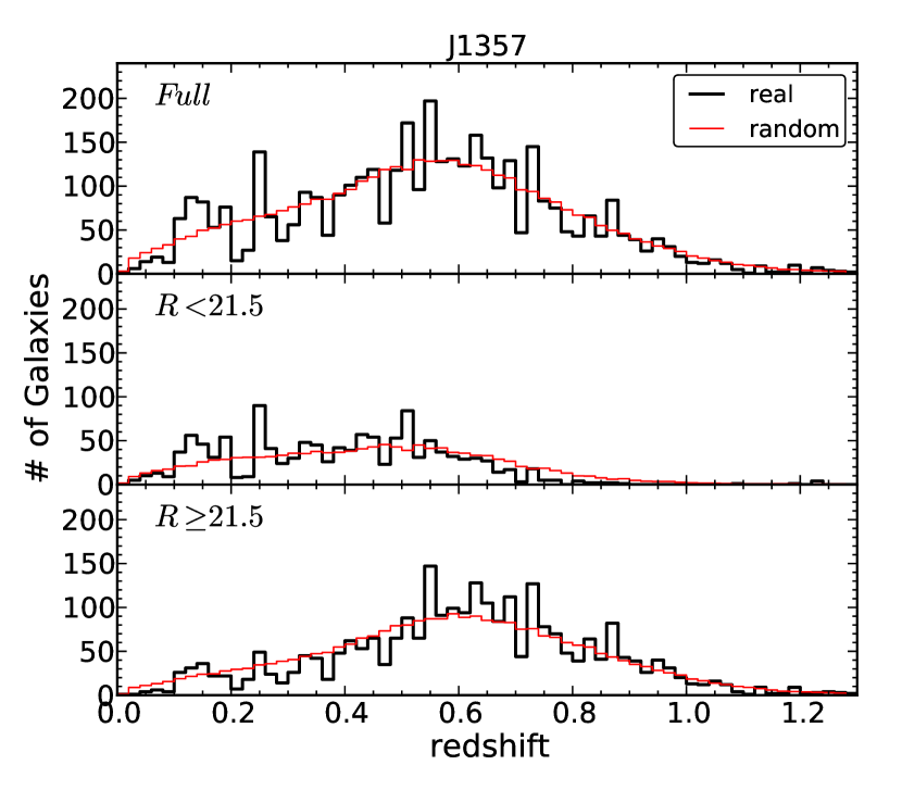
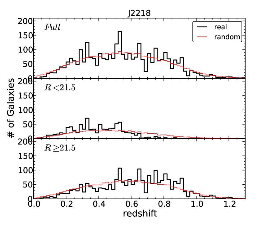
Figure 12: Histograms of the galaxy redshift distribution for our different fields ($0.02$ binning). The black thick solid lines correspond to the real distributions whereas the red thin solid lines correspond to the normalized random expectation drawn from samples of $20\times$ the real sample sizes. A full description of the random generator algorithm can be found in Section 6.2.2. Top panels show the full galaxy samples while the middle and bottom panels show subsamples based on $R$-band magnitude cuts.

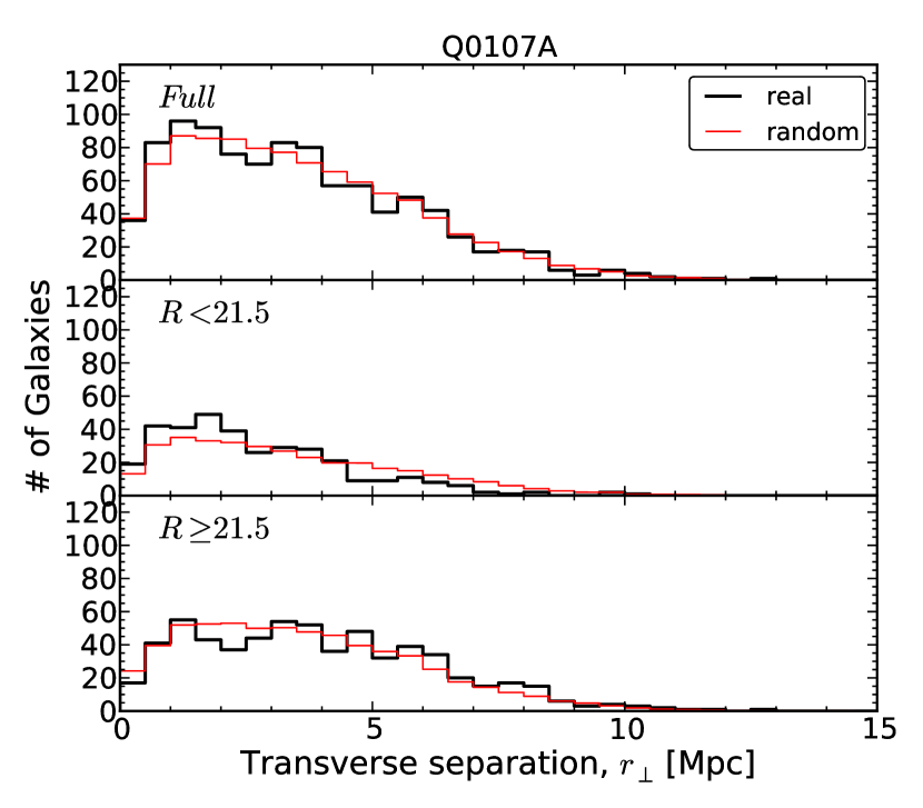
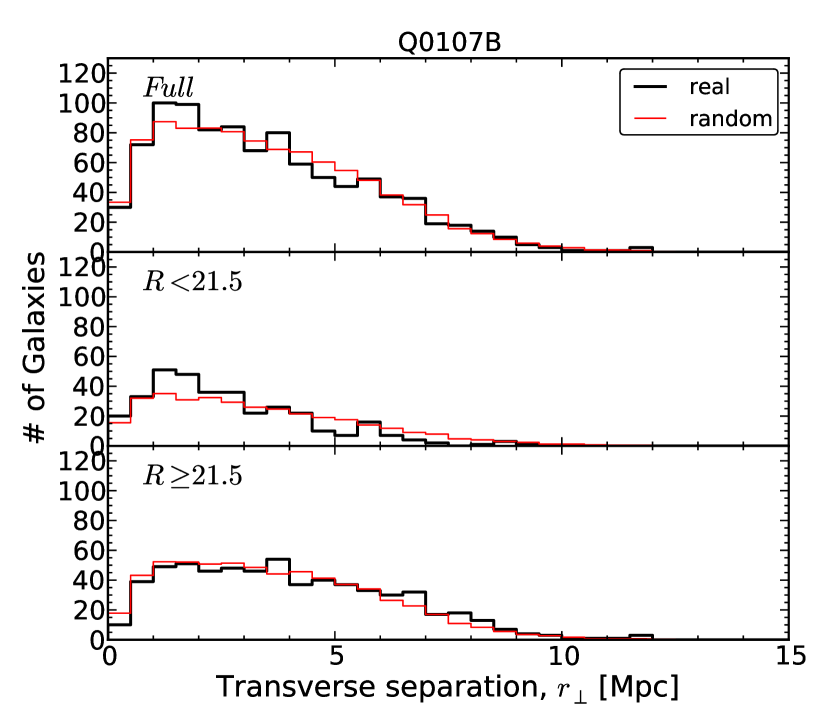
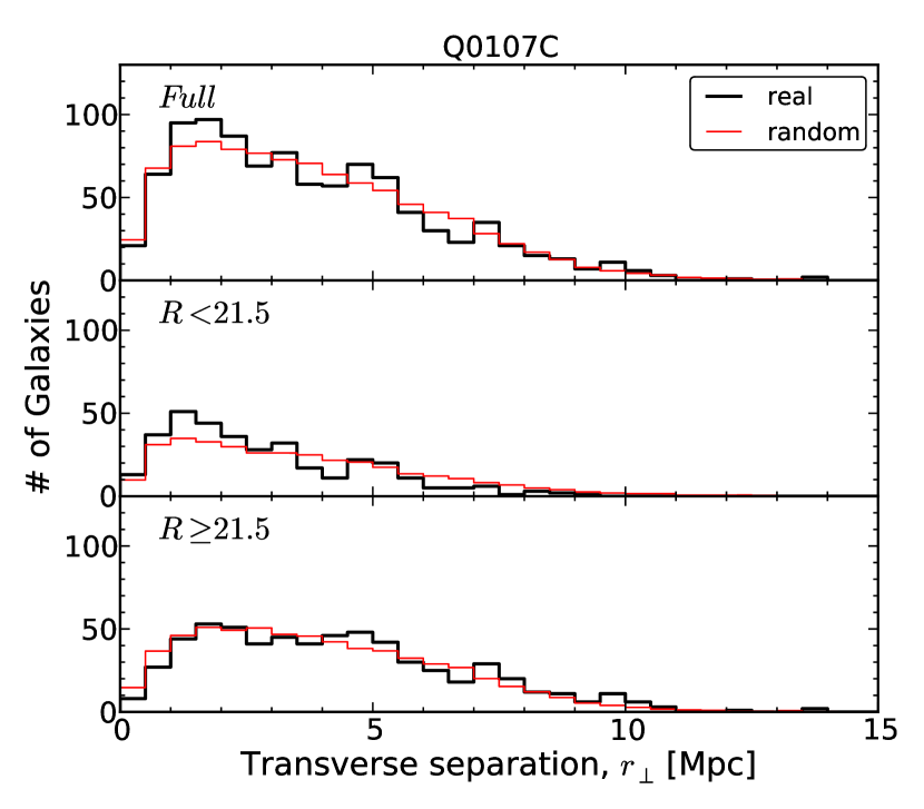
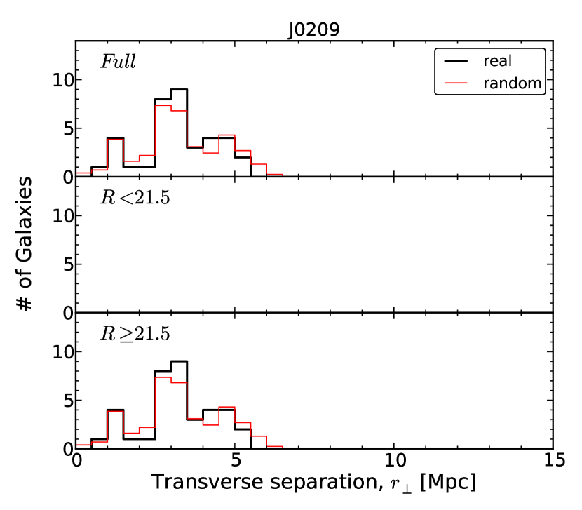
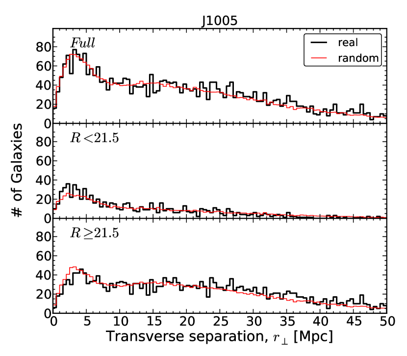
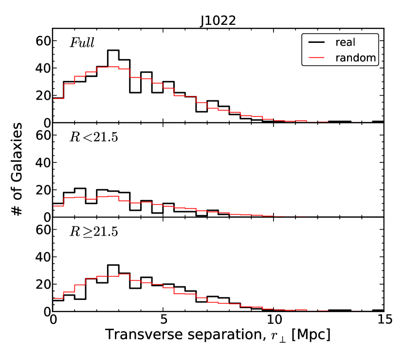
Figure 13: Histograms of the galaxy transverse separation distribution for our different fields ($0.5$  Mpc binning). The black thick solid lines correspond to the real distributions whereas the red thin solid lines correspond to the normalized random expectation drawn from samples of $20\times$ the real sample sizes. A full description of the random generator algorithm can be found in Section 6.2.2. Top panels show the full galaxy samples while the middle and bottom panels show subsamples based on $R$-band magnitude cuts.

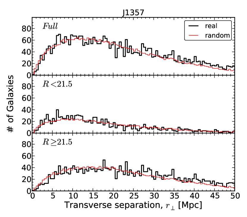
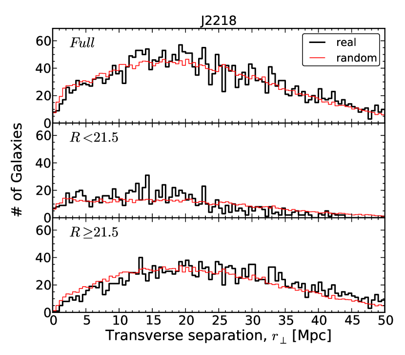
Figure 14: continued

6.2.1 Random absorption lines

We created random samples for individual observations made with a given instrument and/or instrument setting (i.e. resolution, wavelength coverage, etc). This means that we treat the two channels of COS (FUV and NUV) independently for the creation of the random samples, and also for FOS. For a given absorption system with (RA, DEC, $z_{\rm abs}$, $N_{\rm HI}$, $b_{\rm HI}$) we create $\alpha_{\rm abs}$ random ones, varying the redshift but preserving the rest of its parameters.

The random redshifts were chosen based on the properties of the spectrum in which the original absorption system was observed. We first estimated the minimum rest-frame equivalent width of a transition that could have been observed in the spectrum at a redshift $z$. For unresolved features, the minimum equivalent width for a line to be detected at wavelength $\lambda$ is

$$W_{\rm min}(\lambda)\approx sl\ \frac{\rm FWHM}{\langle S/N\rangle_{\lambda}}\ \rm{,}$$ (14)

where $sl$ is the significance level of the detection in standard deviation units, full width at half maximum (FWHM) is the ‘full-width at half maximum’ of the line spread function (LSF) of the spectrograph in Å, and $\langle S/N\rangle_{\lambda}$ is the average signal-to-noise per resolution element. Transforming $\lambda$ coordinates to redshift coordinates for a given rest-frame transition at $\lambda_{0}$ (i.e. $\lambda\ \rightarrow\ z=\frac{\lambda}{\lambda_{0}}-1$), and assuming a constant spectral resolution $R\equiv\frac{\lambda}{\rm FWHM}$, the rest-frame minimum equivalent width is then given by

$$W_{\rm r,min}(z)\approx sl\frac{\lambda_{0}}{R\langle S/N\rangle_{z}}\ \rm{.}$$ (15)

Finally, for a given absorber with equivalent width, $W_{\rm HI}^{\rm obs}$, we compare it with $W_{\rm r,min}(z)$ and place $\alpha_{\rm abs}$ random absorbers uniformly at redshifts where the condition $W_{\rm HI}^{\rm obs}\geq W_{\rm r,min}(z)$ is satisfied. We masked out spectral regions over a velocity window of $\pm 200$  around the position where strong Galactic absorption could have been detected (namely: C 2, N 5, O 1, Si 2, P 3, S 2 and Fe 2) before the random redshifts are assigned.

Even though we have direct measurements of the equivalent widths for the real absorption systems, we do not use them directly in order to avoid confusion from blended systems. We use instead the approximation given by Draine (2011, see his equation 9.27) to convert the inferred $N_{\rm HI}$ and $b_{\rm HI}$ to a $W_{\rm HI}^{\rm obs}$. Note that passing from $W_{\rm HI}\rightarrow(N_{\rm HI},b_{\rm HI})$ is not always robust because of the flat part of the curve-of-growth, but passing from $(N_{\rm HI},b_{\rm HI})\rightarrow W_{\rm HI}$ is.

We mainly based our search of H i absorption systems on the  transition (for which $\lambda_{0}=1215.67$ Å), but in some cases we extended it to  in spectral regions with no  coverage. For the  detected systems, we applied the same method described above but changing the transition parameters accordingly.

Figure 11 presents the redshift distribution of real (black lines) and random (red lines) absorbers in each of our independent fields using $\alpha_{\rm abs}$ $=200$.

6.2.2 Random galaxies

The random galaxies were created for each field and instrument independently. This means that we treat different galaxy surveys independently for the creation of the random samples, even when the galaxy surveys come from the same field. For a given observed galaxy with (RA, DEC, $z_{\rm gal}$, magnitude, spectral type, etc.) we create $\alpha_{\rm gal}$ random ones, varying the redshift, but preserving the rest of its parameters. This approach ensures the selection function is well matched by the random galaxies.

The random redshifts ($z_{\rm gal}^{\rm rand}$) were chosen based on the observed redshift distribution. We made sure that our randoms resembled the observed galaxy distribution independently of the observed magnitude of the galaxies. To do so, we selected multiple subsamples of galaxies at different magnitude bins, whose empirical redshift distributions are used as proxies for the redshift selection function. We used magnitude bins of size $1$, shifted by $0.5$ magnitudes, ranging from $15$ to $25$. For the brighter and fainter ends of the subsamples we increased the magnitude bin sizes to ensure a minimum of $20$ galaxies. For each magnitude subsample, we computed histograms using redshift bins of $\Delta z=0.01$ (arbitrary), which were then smoothed with a Gaussian filter of standard deviation $\sigma=0.1$ (roughly corresponding to a co-moving scale of $\approx 300$  Mpc at redshift $z=0.5$). This large smoothing length is important to get rid of the LSS spikes and valleys present in the real redshift distributions. The final redshift probability distribution of a given magnitude bin is obtained by cubic spline interpolation over the smoothed histograms. Thus, for a given galaxy with observed magnitude $m$, we placed $\alpha_{\rm gal}$ randoms according to the spline fit associated with the subsample of galaxies centred on the closest magnitude bin to $m$. We also imposed the redshifts of the random galaxies to lie between $z_{\rm min}<z_{\rm gal}^{\rm random}<z_{\rm max}$, where $z_{\rm min}$ and $z_{\rm max}$ are the minimum and maximum galaxy redshifts of the real sample.

Figure 12 presents the redshift distribution of real (black lines) and random (red lines) galaxies in each of our independent fields using $\alpha_{\rm gal}$ $=20$. Similarly, Figure 13 presents the distribution in transverse separations of real (black lines) and random (red lines) galaxies with respect to their respective QSO LOS.

6.3 Projected correlations along the line-of-sight

A useful quantity to compute from the two-dimensional correlation functions is the projected correlation function along the LOS,

$$\Xi(r_{\perp})=2\int_{0}^{\infty}\!\xi(r_{\perp},r_{\parallel})\,{\rm d}r_{\parallel}\ \rm{,}$$ (16)

as it will be insensitive to redshift distortions, at least for the transverse separations involved in this work (Davis & Peebles, 1983). Therefore, one can find a relation between the ‘real-space’ correlation function (distortion free), $\xi(r=\sqrt{r_{\parallel}^{2}+r_{\perp}^{2}})$, and $\Xi(r_{\perp})$, as

$$\begin{split}\Xi(r_{\perp})&=2\int_{0}^{\infty}\!\xi(r)\,{\rm d}r_{\parallel}\\ &=2\int_{r_{\perp}}^{\infty}\!\xi(r)\frac{r\,{\rm d}r}{\sqrt{r^{2}-r_{\perp}^{2}}}\ \rm{,}\end{split}$$ (17)

which leads to $\xi(r)$ being given by the inverse Abel transform,

$$\xi(r)=-\frac{1}{\pi}\int_{r}^{\infty}\!\frac{{\rm d}\Xi(r_{\perp})}{{\rm d}r_{\perp}}\frac{{\rm d}r_{\perp}}{\sqrt{r_{\perp}^{2}-r^{2}}}\ \rm{.}$$ (18)

Davis & Peebles (1983) showed that when $\xi(r)$ is described by a power-law of the form,

$$\xi(r)=\left(\frac{r}{r_{0}}\right)^{-\gamma}\ \rm{,}$$ (19)

then Equation 17 yields to

$$\Xi(r_{\perp})=A(r_{0},\gamma)r_{\perp}^{1-\gamma}\ \rm{,}$$ (20)

where $A(r_{0},\gamma)=r_{0}^{\gamma}\Gamma(1/2)\Gamma[(\gamma-1)/2]/\Gamma(\gamma/2)$ and $\Gamma$ is the Gamma function. Therefore, $r_{0}$ and $\gamma$ of $\xi(r)$ can be obtained directly from a power-law fit to $\Xi(r_{\perp})$, using Equation 20. Note that this method is only valid for $\gamma>1$.

In practice, we will use $r_{\parallel}^{\rm max}=20$  Mpc as the integration limit in Equation 16. A larger integration limit will increase the ‘shot noise’ while not adding much correlation power. As long as the vast majority of correlated pairs are included in the integration limit (which is the case), this approach will suffice (e.g. Davis & Peebles, 1983; Ryan-Weber, 2006). In order to further reduce the ‘shot noise’, we summed all the cross-pairs along the LOS, e.g. $D_{\rm a}D_{\rm g}(r_{\perp})=\sum_{i}D_{\rm a}D_{\rm g}(r_{\perp},r_{\parallel,i})$ (and so on for the others), and then computed the Landy & Szalay estimators, $\xi^{\rm LS}(r_{\perp})$, using these collapsed cross-pairs,

$$\Xi(r_{\perp})=2r_{\parallel}^{\rm max}\xi^{\rm LS}(r_{\perp})\ \rm{.}$$ (21)

This approach is justified given the cylindrical geometry of our survey, for which the ‘random-random’ pairs (denominator of the LS estimator) is almost constant along the $r_{\parallel}$-axis for the scales involved in this study (e.g. see right panel of Figure 10). We compared the absolute values of $\Xi$ from our adopted approach with that of a direct integration (as in Equation 16 using $r_{\parallel}^{\rm max}=20$  Mpc as the integration limit). We obtained differences of $\lesssim 5\%$ in the correlation amplitudes, indicating that our approach is appropriate.

6.4 Relations between auto- and cross-correlations

We use the Cauchy–-Schwarz inequality,

$$\xi_{\rm ag}^{2}\leq\xi_{\rm gg}\xi_{\rm aa}\rm{,}$$ (22)

as the main tool to address the connection between H i and galaxies. The equality only holds when the density fluctuations that give rise to H i absorption systems and galaxies are linearly dependent. However, in the most general case, the product of the auto-correlation functions does not necessarily equal $\xi_{\rm ag}^{2}$. If we do assume that both H i absorption systems and galaxies trace the same underlying dark matter density distribution (e.g. Ryan-Weber, 2006), we have

$$\begin{split}\xi_{\rm gg}&=b_{\rm g}^{2}\xi_{\rm DM}\\ \xi_{\rm aa}&=b_{\rm a}^{2}\xi_{\rm DM}\\ \xi_{\rm ag}&=b_{\rm a}b_{\rm b}\xi_{\rm DM}\rm{,}\end{split}$$ (23)

where $\xi_{\rm DM}$ is the dark matter auto-correlation function (assumed positive) and $b_{\rm g}$ and $b_{\rm a}$ are the galaxy and H i ‘absolute biases’ (also positives), respectively. If these biases are independent of the scale (i.e. linear biases), then the equality of Equation 22 holds. If that is the case, one can use the ratio between the correlation functions to infer the dark matter halo masses of one population relative to the other (e.g. Mo, Peacock & Xia, 1993; Ryan-Weber, 2006). On the other hand, if $\xi_{\rm ag}^{2}<\xi_{\rm gg}\xi_{\rm aa}$ we can no longer assume such a simplistic model. In such a case, the observed difference with respect to $\xi_{\rm ag}^{2}=\xi_{\rm gg}\xi_{\rm aa}$ can be used to: (i) get insights on the baryonic physics affecting H i absorption systems and/or galaxies, assuming that the standard cosmological paradigm is correct; or (ii) put constraints on the current cosmological paradigm, assuming that the baryonic physics is fully understood. In this paper we will focus on the former.

Adelberger et al. (2003) showed a third possibility: $\xi_{\rm ag}^{2}$ exceeding $\xi_{\rm gg}\xi_{\rm aa}$ for correlation functions measured from discrete and volume limited samples. In the hypothetical case of an H i–galaxy one-to-one correspondence, then $\xi_{\rm gg}=\xi_{\rm aa}$, but $\xi_{\rm ag}$ will appear higher at the very small scales because in the case of auto-correlations we exclude the correlation of an object with itself, whereas in $\xi_{\rm ag}$ that correlation is present (Adelberger et al., 2003, see their appendix A). Such a behaviour between auto- and cross-correlations will indicate that the two populations of objects are indeed the same physical entities. The geometry of our survey might not be suitable for testing this idea, as we are only mapping H i absorption systems along single LOS for which the completeness level of galaxies close to these absorbers is low. Still, we will bear this result in mind for the interpretation of our results.

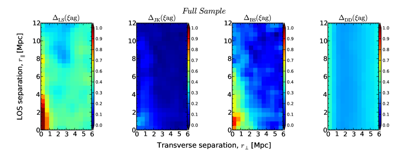
Figure 15: Uncertainty estimations (square root of variances) of the H i-galaxy cross-correlation, $\Delta(\xi^{\rm LS}_{\rm ag})$, measured from our ‘Full Sample’ as a function of separations both along the line-of-sight ($r_{\parallel}$; $y$-axes) and transverse to the line-of-sight ($r_{\perp}$; $x$-axes). From left to right: uncertainty from the Landy & Szalay (1993) analytical approximation, $\Delta_{\rm LS}$ (equation 24); uncertainty from a ‘jackknife’ resampling, $\Delta_{\rm JK}$ (equation 26); uncertainty from a ‘bootstrap’ resampling, $\Delta_{\rm BS}$ (equation 27); and the commonly used Poissonian uncertainty, $\Delta_{\rm DD}$ (equation 25).

6.5 Uncertainty estimation

When dealing with cross-correlations, it is important to realize that the statistical uncertainties will be dominated by those of the smallest sample. If we consider a sample composed of a single object and another sample composed of $100$ objects, the number of cross-pairs is $100$, but none of these pairs are truly independent as they all share a common object. Therefore, assuming Poissonian uncertainty for the number of pairs (as commonly done in the literature; e.g. Chen & Mulchaey, 2009) is not optimal, as it will underestimate the true uncertainty. For correlated distributions, none of the pairs are independent because the number of systems at a given scale will depend on the number of systems at all other scales, and deviations from the Poissonian expectation will be more important at the scales where the correlation signal is large. Indeed, Landy & Szalay (1993) showed that the variance of $\xi^{\rm LS}$ can be approximated by (in our notation),

$$\Delta^{2}_{\rm LS}(\xi^{\rm LS})\approx\frac{(1+\xi^{\rm LS})^{2}}{n_{\rm DD}(RR/n_{\rm RR})}\approx\frac{(1+\xi^{\rm LS})^{3}}{DD}\ \rm{.}$$ (24)

This variance is greater than the commonly used

$$\Delta^{2}_{\rm DD}(\xi^{\rm LS})=\frac{1+\xi^{\rm LS}}{DD}\ \rm{,}$$ (25)

by a factor of $\sim(1+\xi)^{2}$, and so we caution the use of the latter as it might still underpredict the real uncertainty.

In order to test whether the uncertainty given by Equation 24 is reasonable for our survey, we also computed the ‘jackknife’ and ‘bootstrap’ variances. The ‘jackknife’ variance is computed as

$$\Delta^{2}_{\rm JK}(\xi)=\frac{1}{N_{\rm f}(N_{\rm f}-1)}\sum\limits_{i}^{N_{\rm f}}(\xi^{*}_{i}-\bar{\xi}^{*})^{2}\ \rm{,}$$ (26)

where $\xi^{*}_{i}$ is the $i$-th ‘pseudo-value’ of the correlation function, $\xi^{*}_{i}\equiv N_{\rm f}\xi-(N_{\rm f}-1)\xi_{-i}$, with $\xi_{-i}$ being the value of the correlation function measured when the $i$-th field is removed from the sample, and $\bar{\xi}^{*}$ is the mean of the ‘pseudo-values’. The ‘bootstrap’ variance is computed by creating $N_{\rm bs}=500$ sets of $N_{\rm f}$ fields, randomly chosen (with repetition) from the set of real fields, so

$$\Delta^{2}_{\rm BS}(\xi)=\frac{1}{N_{\rm bs}}\sum\limits_{i}^{N_{\rm bs}}(\xi_{i}-\bar{\xi})^{2}\ \rm{,}$$ (27)

where $\xi_{i}$ is the correlation measured from the $i$-th random set, and $\bar{\xi}$ is the mean of these ‘bootstrap’ measurements. Uncertainties for the projected correlations, $\Xi$, and the ratio $(\xi_{\rm ag})^{2}/(\xi_{\rm gg}\xi_{\rm aa})$, were calculated analogously.

As an example, Figure 15 shows these $4$ uncertainty estimations (square root of the variances) for our measurements of $\xi_{\rm ag}^{\rm LS}(r_{\perp},r_{\parallel})$. From left to right: $\Delta_{\rm LS}$, $\Delta_{\rm JK}$, $\Delta_{\rm BS}$ and $\Delta_{\rm DD}$. All these uncertainty estimations are within $\sim 1$ order of magnitude consistent with each other, but systematic trends are present. $\Delta_{\rm LS}$ and $\Delta_{\rm BS}$ give the largest uncertainties while $\Delta_{\rm JK}$ and $\Delta_{\rm DD}$ give the smallest. We also observe that $\Delta_{\rm LS}$, $\Delta_{\rm JK}$ and $\Delta_{\rm BS}$ peak at the smallest scales (where the correlation amplitudes are greater) while $\Delta_{\rm DD}$ does not. Similar behaviors are observed for the uncertainties associated to our $\xi_{\rm gg}^{\rm LS}(r_{\perp},r_{\parallel})$ measurements (not shown).

Figure 16 shows these $4$ uncertainty estimations for our measurements of the projected correlations $\Xi(r_{\perp})$, for both H i–galaxy (squares) and galaxy–galaxy (circles): $\Delta_{\rm LS}$ (green lines), $\Delta_{\rm JK}$ (red lines), $\Delta_{\rm BS}$ (blue lines) and $\Delta_{\rm DD}$ (yellow lines). The top panel shows the absolute values for these different uncertainties, while the bottom panel shows the ratio of a given uncertainty estimation and $\Delta_{\rm BS}$. As before, we observe systematic trends, but all uncertainties are consistent within $\sim 1$ order of magnitude of each other. In contrast to the two-dimensional uncertainties, $\Delta_{\rm BS}$ is the largest in this case. Focusing on the smallest scales (where the correlation amplitudes are greater) we see that $\Delta_{\rm JK}$ and $\Delta_{\rm LS}$ are in closer agreement to $\Delta_{\rm BS}$ than $\Delta_{\rm DD}$.

Table 6: Summary of the ‘Full Sample’ used for the cross-correlation analysis, as a function of $r_{\perp}$.

	$<0.5$  Mpc	$<1$  Mpc	$<2$  Mpc	$<10$  Mpc	$<50$  Mpc	Total
	(1)	(2)	(3)	(4)	(5)	(6)
Galaxies	141	466	1354	6871	19509	17509
‘SF’	105	339	997	4756	9963	8293
‘non-SF’	24	66	193	779	2011	1743
H i	…	…	…	…	…	654
‘strong’	…	…	…	…	…	165
‘weak’	…	…	…	…	…	489

(1): Number of galaxies at transverse distances $r_{\perp}<0.5$  Mpc from a QSO LOS. (2): Number of galaxies at transverse distances $r_{\perp}<1$  Mpc from a QSO LOS. (3): Number of galaxies at transverse distances $r_{\perp}<2$  Mpc from a QSO LOS. (4) Number of galaxies at transverse distances $r_{\perp}<10$  Mpc from a QSO LOS. (5) Number of galaxies at distances $r_{\perp}<50$  Mpc from a QSO LOS. (6) Total number of galaxies and H i absorption systems in the ‘Full Sample’. Note that the vast majority of galaxies in the triple QSO field Q0107 have been counted three times in columns (1), (2), (3), (4) and (5).

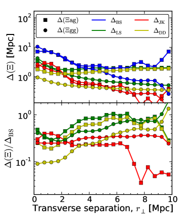
Figure 16: Uncertainty estimations (square root of variances) of the projected H i-galaxy cross-correlation ($\Xi_{\rm ag}$; squares) and galaxy auto-correlation ($\Xi_{\rm gg}$; circles) measured from our full sample as a function of separations transverse to the line-of-sight ($r_{\perp}$). The top panel shows the uncertainty from the Landy & Szalay (1993) analytical approximation, $\Delta_{\rm LS}$ (Equation 24; green lines); uncertainty from a ‘jackknife’ resampling, $\Delta_{\rm JK}$ (Equation 26; red lines); uncertainty from a ‘bootstrap’ resampling, $\Delta_{\rm BS}$ (Equation 27; blue lines); and the commonly used Poissonian uncertainty, $\Delta_{\rm DD}$ (Equation 25; yellow lines). The bottom panel shows the ratio between these uncertainties and $\Delta_{\rm BS}$.

These results suggest that $\Delta_{\rm LS}$ is preferable over $\Delta_{\rm DD}$ and even over $\Delta_{\rm JK}$ (at least when the number of independent fields is small, like in our case). A more in depth study of the error estimation for auto- (e.g. Norberg et al., 2009) and cross-correlations is beyond the scope of this paper.

For the results of this paper, we will adopt uncertainties given by $\Delta_{\rm BS}$. As has been shown, $\Delta_{\rm BS}$ gives, in general, the most conservative uncertainty estimation at all scales. An exception to this rule was found for $\xi_{\rm aa}(r_{\perp},r_{\parallel})$ and $\Xi_{\rm aa}(r_{\perp})$, in which $\Delta_{\rm LS}>\Delta_{\rm BS}$. This is due to the combination of the special survey geometry in which $\xi_{\rm aa}$ is measured. Thus, for such a sample we adopted $\Delta_{\rm LS}$ as the uncertainty.

6.6 Calibration between galaxy and H i absorbers redshift frames

Before computing the final two-point correlation functions, we calibrated the redshift frames between our H i absorption systems and galaxies, using the idea presented by Rakic et al. (2011): that in an isotropic Universe, the mean H i absorption profile around galaxies should be symmetric. Thus, we measured the H i–galaxy cross-correlation using $r_{\parallel,ij}\equiv X_{i}-X_{j}$ instead of $r_{\parallel,ij}\equiv|X_{i}-X_{j}|$, and applied a constant redshift shift to all our galaxies such that the cross-correlation appears symmetric with respect to the $r_{\parallel}=0$ axis at the scales involved in this analysis. This redshift shift corresponded to $+0.0002$ (smaller than the galaxy redshift uncertainty). Note that this shift has not been added to the redshifts reported in Tables 21 to 24. The final two-point correlation functions were still calculated using $r_{\parallel,ij}\equiv|X_{i}-X_{j}|$ in order to reduce the ‘shot noise’.

7 Results

In this section we present the results of the two point correlation analysis, following the formalisms described in Section 6. We used the H i and galaxy samples described in Sections 2, 3, 4 and 5, but excluding: (i) H i and galaxies falling in their respective ‘c’ categories (see Sections 3.1.6 and 4.3); (ii) H i and galaxies at $z<0.01$ and at $z>1.3$; (iii) H i systems at redshifts within $5000$ of the redshift of the QSO in which the absorption line was observed; and (iv) galaxies at projected distances greater than $50$  Mpc from the centre of their closest field. We will refer to this sample as the ‘Full Sample’, which comprises: $654$ H i absorption systems, of which, $165$ are classified as ‘strong’ and $489$ as ‘weak’ (see Section 4.6 for definitions); and $17509$ galaxies, of which, $8293$ are classified as ‘SF’ and $1743$ as ‘non-SF’ (see Section 5.1 for definitions).

Table 6 summarizes relevant information regarding our ‘Full Sample’. The following results were computed with random samples $200\times$ and $20\times$ larger than the real H i and galaxy samples, respectively. Even though we have galaxies up to $50$  Mpc from the QSO LOS, we will focus only on clustering at scales $r_{\perp}<10$  Mpc, as at larger scales our results get considerably noisier. Galaxies at $r_{\perp}>10$ Mpc are still used for the galaxy–galaxy auto-correlation though. In the case of the H i–H i auto-correlation, we only focus on scales $r_{\perp}<2$  Mpc, as we have no data sampling larger transverse scales.

7.1 Two-dimensional correlations

Figure 17: Two-dimensional correlation functions for galaxies and H i absorption system (top panels) and their respective uncertainties (bottom panels), as a function of separations along ($r_{\parallel}$; $y$-axes) and transverse to the line-of-sight ($r_{\perp}$; $x$-axes). From left to right: the galaxy-H i cross-correlation ($\xi_{\rm ag}^{\rm LS}$; equation 8), the galaxy-galaxy auto-correlation ($\xi_{\rm gg}^{\rm LS}$; equation 4), the H i-H i auto-correlation ($\xi_{\rm aa}^{\rm LS}$; equation 6) and the ratio, $(\xi^{\rm LS}_{\rm ag})^{2}/(\xi^{\rm LS}_{\rm gg}\xi^{\rm LS}_{\rm aa})$. Note that our data are not suitable for measuring the $\xi^{\rm LS}_{\rm aa}$ and $(\xi^{\rm LS}_{\rm ag})^{2}/(\xi^{\rm LS}_{\rm gg}\xi^{\rm LS}_{\rm aa})$ at scales $r_{\perp}>2$ Mpc. The correlation functions in this figure were calculated using an arbitrary binning of $0.5$  Mpc with cross-pairs counts smoothed with a Gaussian filter of standard deviation of $0.5$  Mpc along both directions. See Sections 6.1 and 7.1 for further details.

Figure 18: Same as Figure 17 but for ‘SF’ galaxies and H i absorption systems with $N_{\rm HI}\geq 10^{14}$  cm^-2 (‘strong’).

Figure 19: Same as Figure 17 but for ‘non-SF’ galaxies and H i absorption systems with $N_{\rm HI}\geq 10^{14}$  cm^-2 (‘strong’).

Figure 20: Same as Figure 17 but for ‘SF’ galaxies and H i absorption systems with $N_{\rm HI}<10^{14}$  cm^-2 (‘weak’).

Figure 21: Same as Figure 17 but for ‘non-SF’ galaxies and H i absorption systems with $N_{\rm HI}<10^{14}$  cm^-2 (‘weak’).

7.1.1 Full Sample

In Figure 17 we show the two-dimensional correlation functions (top panels) and their respective uncertainties (bottom panels) for our ‘Full Sample’ of H i-absorption systems and galaxies. The first three panels, from left to right, show the H i–galaxy cross-correlation ($\xi_{\rm ag}^{\rm LS}$; Equation 8), the galaxy–galaxy auto-correlation ($\xi_{\rm gg}^{\rm LS}$; Equation 4) and the H i–H i auto-correlation ($\xi_{\rm aa}^{\rm LS}$; Equation 6), respectively. We see that the amplitudes of $\xi_{\rm ag}$ and $\xi_{\rm aa}$ are comparable (within the uncertainties), whereas the amplitude of $\xi_{\rm gg}$ is greater than these two (see also Table 7). Also, the fact that both $\xi_{\rm gg}$ and $\xi_{\rm ag}$ peak at the smallest separations confirms that the redshift frames for H i absorption systems and galaxies are self consistent (by construction; see Section 6.6). The decrease in the $\xi_{\rm aa}$ signal at the smallest $r_{\parallel}$ separations is because we cannot always resolve two real absorption systems separated by less than the typical width of an absorption feature. This width corresponds to $\sim 16$ ($\sim 100$ ) for FUV (NUV) data, which in co-moving distance correspond to $\sim 0.26$  Mpc ($\sim 1.6$  Mpc) at $z=0.5$.

Our sample of H i absorption systems is not large enough to measure $\xi_{\rm ag}$ or $\xi_{\rm aa}$ anisotropies at a high confidence level. Still, we can obtain qualitative features by looking at the corresponding ‘iso-correlation’ contours. We observe deviations from an isotropic signal in both $\xi_{\rm ag}$ and $\xi_{\rm gg}$. Apart from a decrease of the $\xi_{\rm aa}$ signal at the smallest $r_{\parallel}$ separations, we do not see significant anisotropies in $\xi_{\rm aa}$. The typical uncertainty for our single galaxy redshift determination, $\Delta z_{\rm gal}\approx 0.0006/\sqrt{2}$, is equivalent to $\sim 1.7-1.4$  Mpc at $z=0.1-0.5$, which corresponds to an ‘anisotropy ratio’ of $\sim 3:1$ for pixels of $0.5$  Mpc each. If the observed anisotropies are dominated by redshift uncertainties, we should expect the $\xi_{\rm ag}$ contours to be consistent with this ratio (neglecting the much smaller contribution from the H i redshift uncertainty) and the $\xi_{\rm gg}$ one to be $\sim 4:1$ (greater by a factor of $\sqrt{2}$). These expectations are consistent with what we see in our ‘Full Sample’ for the smallest scales, whereas for scales $\gtrsim 4$  Mpc the anisotropy looks somewhat reduced. We do not detect compression along the LOS at larger scales either (e.g. Kaiser, 1987). The only anisotropy observed can be fully explained by galaxy redshift uncertainties.

The fourth panel of Figure 17 shows the ratio, $(\xi^{\rm LS}_{\rm ag})^{2}/(\xi^{\rm LS}_{\rm gg}\xi^{\rm LS}_{\rm aa})$. We see that the majority of the bins at the smallest scales have values $(\xi_{\rm ag})^{2}/(\xi_{\rm gg}\xi_{\rm aa})<1$. This result suggests that, contrary to what is usually assumed, the population of H i absorption systems (as a whole) and galaxies do not linearly trace the same underlying dark matter distributions (see Section 6.4).

In the following, we will split the H i absorber sample into ‘strong’ ($N_{\rm HI}\geq 10^{14}$  cm^-2) and ‘weak’ ($N_{\rm HI}<10^{14}$  cm^-2), and the galaxy sample into ‘SF’ and ‘non-SF’. In this way we can isolate the contribution of each sub-population of H i and galaxies to the correlation functions, and to the $(\xi_{\rm ag})^{2}/(\xi_{\rm gg}\xi_{\rm aa})$ ratio.

7.1.2 ‘Strong’ H i systems and ‘SF’ galaxies

Figure 18 is analogous to Figure 17 but for ‘strong’ H i systems ($N_{\rm HI}\geq 10^{14}$  cm^-2) and ‘SF’ galaxies. We see that in this case the $\xi_{\rm ag}$, $\xi_{\rm gg}$ and $\xi_{\rm aa}$ are all comparable within the errors (see also Table 7). Anisotropy signals behave in the same way as for our ‘Full Sample’, i.e. are dominated by our galaxy redshift uncertainty and with no detected compression along the LOS at large scales.

In this case, the ratio $(\xi_{\rm ag})^{2}/(\xi_{\rm gg}\xi_{\rm aa})$ is consistent with $1$, suggesting that ‘SF’ galaxies and $N_{\rm HI}$ $\geq 10^{14}$  cm^-2 systems do trace the same underlying dark matter distribution. The comparable clustering amplitudes may also indicate that they typically belong to dark matter haloes of similar masses. We will address these points more quantitatively in Section 7.2

7.1.3 ‘Strong’ H i systems and ‘non-SF’ galaxies

Figure 19 shows the correlation functions for ‘strong’ H i systems ($N_{\rm HI}\geq 10^{14}$  cm^-2) and ‘non-SF’ galaxies. In this case, $\xi_{\rm ag}$, $\xi_{\rm gg}$ and $\xi_{\rm aa}$ are all comparable within the errors (see also Table 7), but $\xi_{\rm gg}$ appears systematically larger. As before, the anisotropy is dominated by the galaxy redshift uncertainty and no (significant) compression along the LOS at large scales is detected.

Interestingly, there is a displacement in the $\xi_{\rm ag}$ peak relative to the smallest bin. This signal also appears symmetric with respect to the $r_{\parallel}=0$ axis, after computing $\xi_{\rm ag}$ using $r_{\parallel,ij}\equiv X_{i}-X_{j}$ (not plotted) instead of $r_{\parallel,ij}\equiv|X_{i}-X_{j}|$. We also checked that the signal remained using only ‘a’ labelled H i systems and galaxies. This suggests that this feature might be real. A similar (although more uncertain) feature was observed by Wilman et al. (2007), from their observation of the H i-‘absorption-line-dominated galaxy’ cross-correlation (see their figure 4). Pierleoni, Branchini & Viel (2008) also reported a similar signal from hydrodynamical simulations (see their figure 7), although their samples of H i and galaxies are not directly comparable to our ‘strong’ and ‘non-SF’ ones. A more detailed comparison between our results and those from previous studies will be presented in Section 8.1.

The ratio $(\xi_{\rm ag})^{2}/(\xi_{\rm gg}\xi_{\rm aa})$ seems also consistent with $1$, which suggests that ‘non-SF’ galaxies and $N_{\rm HI}$ $\geq 10^{14}$  cm^-2 systems trace the same underlying dark matter distribution linearly.

Comparing Figures 18 and 19 we see that $\xi_{\rm gg}$ for ‘non-SF’ galaxies is larger than that of ‘SF’ galaxies (as has been shown by many authors). Given that $\xi_{\rm aa}$ is the same in both cases, one would expect $\xi_{\rm ag}$ to be also larger for ‘non-SF’ than that of ‘SF’ galaxies. Although within the uncertainties our results indicate that the $\xi_{\rm ag}$ amplitude is independent of galaxy type, we do see a somewhat larger cross-correlation signal for ‘non-SF’ galaxies (see Table 7). We will address these points more quantitatively in Section 7.2.

7.1.4 ‘Weak’ H i systems and galaxies

Figures 20 and 21 show the two-dimensional correlation functions for ‘weak’ H i absorption systems ($N_{\rm HI}<10^{14}$  cm^-2) and ‘SF’ and ‘non-SF’ galaxies, respectively. These results are dramatically different than those for ‘strong’ H i systems and galaxies. In particular, $\xi_{\rm ag}$ is significantly weaker than $\xi_{\rm gg}$ but also weaker than $\xi_{\rm aa}$, for both types of galaxies. Consequently, the ratios $(\xi_{\rm ag})^{2}/(\xi_{\rm gg}\xi_{\rm aa})$ are both smaller than one. This is a very strong indication (given the comparatively smaller uncertainties) that the underlying baryonic matter distributions giving rise to ‘weak’ H i absorption systems and galaxies are not linearly dependent. Given that the signal in the $\xi_{\rm ag}$ is marginally consistent with zero, we do not observe anisotropies either.

To summarize, ‘strong’ systems and galaxies are consistent with tracing the same underlying dark matter distribution linearly, whereas ‘weak’ systems are not. Therefore, the fact that $(\xi_{\rm ag})^{2}/(\xi_{\rm gg}\xi_{\rm aa})<1$ in the ‘Full Sample’ should be primarily driven by the presence of H i systems with $N_{\rm HI}<10^{14}$  cm^-2. We also note that the amplitude of $\xi_{\rm aa}$ is weaker for ‘weak’ systems than that for ‘strong’ systems.

Because redshift uncertainties affect $\xi_{\rm ag}$, $\xi_{\rm gg}$ and $\xi_{\rm aa}$ in different ways, the interpretation of the two-dimensional $(\xi_{\rm ag})^{2}/(\xi_{\rm gg}\xi_{\rm aa})$ is not straightforward. In the following we present the results for the projected correlation functions, which are not affected by velocity distortions along the LOS, and have smaller statistical uncertainties.

Table 7: Strength of the two-dimensional correlations, $\xi(r_{\perp},r_{\parallel})$, at their peaks.

	$\xi_{\rm ag}^{\rm peak}$	$\xi_{\rm gg}^{\rm peak}$	$\xi_{\rm aa}^{\rm peak}$
Full Sample	2.3 $\pm$ 0.9	5.7 $\pm$ 0.7	2.1 $\pm$ 0.9
‘Strong’–‘SF’	8.3 $\pm$ 2.2	6.1 $\pm$ 0.6	7.5 $\pm$ 2.3
‘Strong’–‘non-SF’	10.3 $\pm$ 5.6	12.6 $\pm$ 3.0	7.5 $\pm$ 2.3
‘Weak’–‘SF’	0.9 $\pm$ 0.6	6.1 $\pm$ 0.6	1.9 $\pm$ 0.9
‘Weak–‘non-SF’	0.6 $\pm$ 0.5	12.6 $\pm$ 3.0	1.9 $\pm$ 0.9

^a Note that peaks are not necessarly at the smallest scale bins (see Figures 17 to 21).

7.2 Correlations projected along the line-of-sight

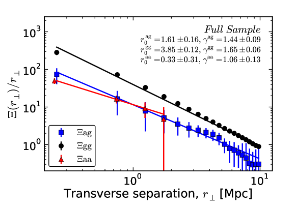
Figure 22: Projected along the line-of-sight correlation functions (see equation 16) divided by the transverse separation, $\Xi(r_{\perp})/r_{\perp}$, for our ‘Full Sample’ of galaxies and H i absorption systems. Different symbols/colors show our different measurements: the blue squares correspond to the galaxy-H i cross-correlation ($\Xi_{\rm ag}$); the black circles to the galaxy-galaxy auto-correlation ($\Xi_{\rm gg}$); and the red triangles to the H i-H i auto-correlation ($\Xi_{\rm aa}$; slightly shifted along the $x$-axis for the sake of clarity). The lines correspond to the best power-law fits (Equation 20) to the data, from a non-linear least squares analysis. The parameters $r_{0}$ and $\gamma$ correspond to those of the real-space correlation function, $\xi(r)$, when described as a power-law of the form presented in Equation 19. Note that points and uncertainties are both correlated, and that uncertainties smaller than the symbols are not shown.

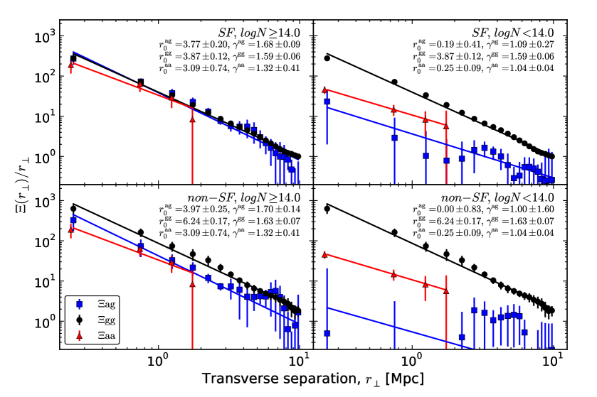
Figure 23: Same as Figure 22 but for our different subsamples: ‘SF’ galaxies and ‘strong’ ($N_{\rm HI}\geq 10^{14}$  cm^-2) H i absorption systems (top left); ‘SF’ galaxies and ‘weak’ ($N_{\rm HI}<10^{14}$  cm^-2) H i absorption systems (top right); ‘non-SF’ galaxies and ‘strong’ H i absorption systems (bottom left); and ‘non-SF’ galaxies and ‘weak’ H i absorption systems (bottom right). Note that points and uncertainties are both correlated, and that uncertainties smaller than the symbols are not shown.

Table 8: Best fit parameters to the real-space correlation function assuming power-law of the form presented in Equation 19.

. $\xi_{\rm ag}(r)$ $\xi_{\rm gg}(r)$ $\xi_{\rm aa}(r)$ $r_{0}$ ( Mpc) $\gamma$ $r_{0}$ ( Mpc) $\gamma$ $r_{0}$ ( Mpc) $\gamma$ Full Sample 1.6 $\pm$ 0.2 1.4 $\pm$ 0.1 3.9 $\pm$ 0.1 1.7 $\pm$ 0.1 0.3 $\pm$ 0.3 1.1 $\pm$ 0.1     ‘Strong’–‘SF’ 3.8 $\pm$ 0.2 1.7 $\pm$ 0.1 3.9 $\pm$ 0.1 1.6 $\pm$ 0.1 3.1 $\pm$ 0.7 1.3 $\pm$ 0.4     ‘Strong’–‘non-SF’ 4.0 $\pm$ 0.3 1.7 $\pm$ 0.1 6.2 $\pm$ 0.2 1.6 $\pm$ 0.1 3.1 $\pm$ 0.7 1.3 $\pm$ 0.4     ‘Weak’–‘SF’ 0.2 $\pm$ 0.4 1.1 $\pm$ 0.3 3.9 $\pm$ 0.1 1.6 $\pm$ 0.1 0.3 $\pm$ 0.1 1.0 $\pm$ 0.1     ‘Weak–‘non-SF’ 0.0 $\pm$ 0.8 1.0 $\pm$ 1.6 6.2 $\pm$ 0.2 1.6 $\pm$ 0.1 0.3 $\pm$ 0.1 1.0 $\pm$ 0.1

7.2.1 Full Sample

Figure 22 shows the projected (along the LOS; see Equation 16) correlation functions divided by the transverse separation, $\Xi(r_{\perp})/r_{\perp}$, for our ‘Full Sample’ of H i absorption systems and galaxies. Different symbols/colors show our different measurements: the blue squares correspond to the H i–galaxy cross-correlation ($\Xi_{\rm ag}$), the black circles to the galaxy–galaxy auto-correlation ($\Xi_{\rm gg}$), and the red triangles to the H i–H i auto-correlation ($\Xi_{\rm aa}$; slightly shifted along the $x$-axis for the sake of clarity). The lines correspond to the best power-law fits (Equation 20) to the data, from a non-linear least squares analysis. The parameters $r_{0}$ and $\gamma$ correspond to those of the real-space correlation function, $\xi(r)$, when described as a power-law of the form presented in Equation 19. Uncertainties in these fits include the variances and covariances of both parameters. From this figure, we see that a power-law fit is a good description of the data, hence justifying the use of Equations 19 and 20. Table 8 summarizes the best power-law fit parameters for our different samples.

We find that $\xi_{\rm ag}(r)$ has a correlation length of $r_{0}^{\rm ag}=1.6\pm 0.2$  Mpc and slope $\gamma^{\rm ag}=1.4\pm 0.1$, whereas $\xi_{\rm gg}(r)$ and $\xi_{\rm aa}(r)$ have correlation lengths of $r_{0}^{\rm gg}=3.9\pm 0.1$  Mpc and $r_{0}^{\rm aa}=0.3\pm 0.3$  Mpc, and slopes $\gamma^{\rm gg}=1.7\pm 0.1$, $\gamma^{\rm aa}=1.1\pm 0.1$, respectively. Thus, the clustering of H i absorption systems and galaxies is weaker than the clustering of galaxies with themselves, and the clustering of H i systems with themselves is weaker still. We also see that the slopes are inconsistent with each other at the $1\sigma$ confidence level (c.l.), which is in tension with the assumption that these objects trace the same underlying dark matter distribution linearly (see Section 6.4). Moreover, the slope of the $\xi_{\rm aa}(r)$ is consistent with $\gamma=1$, indicating that this distribution is at the limit in which the methodology adopted here is valid (see Section 6.3).

As was the case for the two-dimensional results, in the following we will split the H i and galaxy samples into ‘weak’ and ‘strong’, and ‘SF’ and ‘non-SF’, respectively, in order to isolate different contributions from these sub-populations into the observed correlations.

7.2.2 ‘Strong’ H i systems and ‘SF’ galaxies

The top left panel of Figure 23 shows the projected correlation functions for our ‘strong’ H i systems ($N_{\rm HI}\geq 10^{14}$  cm^-2) and ‘SF’ galaxies. In this case, we find that the $\xi_{\rm ag}(r)$ has a correlation length of $r_{0}^{\rm ag}=3.8\pm 0.2$  Mpc and slope $\gamma^{\rm ag}=1.7\pm 0.1$, whereas $\xi_{\rm gg}(r)$ and $\xi_{\rm aa}(r)$ have correlation lengths of $r_{0}^{\rm gg}=3.9\pm 0.1$  Mpc and $r_{0}^{\rm aa}=3.1\pm 0.7$  Mpc, and slopes $\gamma^{\rm gg}=1.6\pm 0.1$, $\gamma^{\rm aa}=1.3\pm 0.4$, respectively (see also Table 8). Thus, all have correlation lengths and slopes agreeing with each other at the $1\sigma$ c.l.. The fact that all have comparable correlation lengths and slopes supports the hypothesis that ‘strong’ H i systems and ‘SF’ galaxies do trace the same underlying dark matter distribution.

7.2.3 ‘Strong’ H i systems and ‘non-SF’ galaxies

The bottom left panel of Figure 23 shows the projected correlation functions for our ‘strong’ H i systems ($N_{\rm HI}\geq 10^{14}$  cm^-2) and ‘non-SF’ galaxies. In this case we find that $\xi_{\rm ag}(r)$ has a correlation length of $r_{0}^{\rm ag}=4.0\pm 0.3$  Mpc and slope $\gamma^{\rm ag}=1.7\pm 0.1$, whereas $\xi_{\rm gg}(r)$ has a correlation length of $r_{0}^{\rm gg}=6.2\pm 0.2$  Mpc and slope $\gamma^{\rm gg}=1.6\pm 0.1$ (see also Table 8). The parameters for $\xi_{\rm aa}(r)$ are the same as in the previous case (see Section 7.2.2). The fact that the slopes are all consistent supports the idea that ‘strong’ H i systems and ‘non-SF’ galaxies also trace the same underlying dark matter distribution. This is an expected result in view of what was observed for the case of ‘strong’ H i systems and ‘SF’ galaxies, and because it is well known that ‘SF’ and ‘non-SF’ do trace the same underlying dark matter distribution. We also see that the galaxy–galaxy auto-correlation is significantly larger than the H i–galaxy cross-correlation and the H i–H i auto-correlation. The most simple explanation for such a difference is that the linear bias (see Section 6.4) of ‘non-SF’ is greater than that of ‘SF’ galaxies. This has been commonly interpreted as ‘non-SF’ galaxies belonging, on average, to more massive dark matter haloes than ‘SF’ galaxies. The fact that the correlation length for the ‘strong’ H i–galaxy cross-correlation is (marginally) larger for ‘non-SF’ than ‘SF’ galaxies is also expected because the H i population is the same in both cases. However, we will see in Section 7.2.5 that this length is smaller than what is expected from the linear dependence hypothesis.

7.2.4 ‘Weak’ H i systems and galaxies

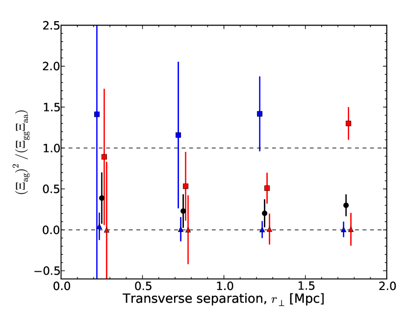
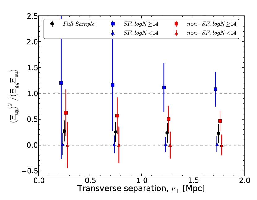
Figure 24: The ratio $(\Xi_{\rm ag})^{2}/(\Xi_{\rm gg}\Xi_{\rm aa})$ as a function of transverse separation, $r_{\perp}$. Results from different samples of galaxies and H i absorption systems are shown by different colors/symbols. The black circles correspond to our ‘Full Sample’; blue and red symbols correspond to ‘SF’ and ‘non-SF’ galaxies respectively; and squares and triangles correspond to ‘strong’ ($N_{\rm HI}\geq 10^{14}$  cm^-2) and ‘weak’ ($N_{\rm HI}<10^{14}$  cm^-2) H i absorption systems respectively. The left panel shows the results from our adopted Gaussian smoothing of $0.5$  Mpc standard deviation while the right panel shows it applying a Gaussian smoothing of $1$  Mpc standard deviation. The smoothings were applied to the cross-pairs only, before calculating the different $\Xi$ and the corresponding ratios (see Section 6). Note that the fifth point associated to ‘strong’ H i systems and ‘SF’ galaxies in the left panel is out of range and hence not shown. Uncertainties were obtained directly from the ‘bootstrap’ resampling technique of our independent fields (see Section 6.5). Note that points and uncertainties are both correlated. For further details see Section 7.2.5.

The top right panel of Figure 23 shows the projected correlation functions for our ‘weak’ H i systems ($N_{\rm HI}<10^{14}$  cm^-2) and ‘SF’ galaxies. In this case we find that $\xi_{\rm ag}(r)$ has a correlation length of $r_{0}^{\rm ag}=0.2\pm 0.4$  Mpc and slope $\gamma^{\rm ag}=1.1\pm 0.3$, whereas $\xi_{\rm aa}(r)$ has a correlation length of $r_{0}^{\rm aa}=0.3\pm 0.1$  Mpc and slope $\gamma^{\rm aa}=1.0\pm 0.1$ (see also Table 8). The parameters for $\xi_{\rm gg}(r)$ are the same as in Section 7.2.2. These results are dramatically different from those involving ‘strong’ H i systems. In particular for the H i–galaxy cross-correlation, not only is the power-law fit questionable, but also the correlation length is smaller than both galaxy–galaxy and H i–H i auto-correlations. Moreover, the correlation length of the cross-correlation is consistent with $r_{0}=0$, i.e., no correlation.

The results for ‘weak’ H i systems and ‘non-SF’ galaxies are even more dramatic. The bottom right panel of Figure 23 shows the projected correlation functions for these samples. In this case we find that $\xi_{\rm ag}(r)$ has a correlation length of $r_{0}^{\rm ag}=0.0\pm 0.8$  Mpc and slope $\gamma^{\rm ag}=1.0\pm 1.6$. Although consistent within errors with the ‘weak’ H i-‘SF’ galaxy cross-correlation, this correlation length is even smaller. This result goes in the opposite direction to what would be expected in the case of linear dependency, because the clustering of ‘non-SF’ galaxies with themselves is stronger than that of ‘SF’. Therefore, these results are a strong indication that ‘weak’ H i systems and galaxies do not trace the same underlying dark matter distribution linearly.

7.2.5 Ratio $(\Xi_{\rm ag})^{2}/(\Xi_{\rm gg}\Xi_{\rm aa})$

Figure 24 shows the ratio $(\Xi_{\rm ag})^{2}/(\Xi_{\rm gg}\Xi_{\rm aa})$ for our different samples. The black circles correspond to our ‘Full Sample’; blue and red symbols correspond to ‘SF’ and ‘non-SF’ galaxies respectively; and squares and triangles correspond to ‘strong’ ($N_{\rm HI}\geq 10^{14}$  cm^-2) and ‘weak’ ($N_{\rm HI}<10^{14}$  cm^-2) H i absorption systems respectively. The left panel shows the results from our adopted Gaussian smoothing of $0.5$  Mpc standard deviation. Given that the points are all correlated, we expected this ratio to be roughly independent of the scale, at least below $\lesssim 2$  Mpc. Thus, we attribute the large variation seen in the left panel of Figure 24 to ‘shot noise’ and repeated the calculation using a Gaussian smoothing of $1$  Mpc standard deviation. The right panel of Figure 24 show the results from this last calculation. We note that the smoothings were applied to the cross-pairs only, before calculating the different $\Xi$ and the corresponding ratios (see Section 6 for details), and that the uncertainties were obtained directly from the ‘bootstrap’ resampling of our independent fields (see Section 6.5).

These results are consistent with what we found for the two-dimensional correlations. We see that the ‘Full Sample’ have ratios inconsistent with $1$. Taking the bin at $1.25$  Mpc as representative, we find that $(\Xi_{\rm ag})^{2}/(\Xi_{\rm gg}\Xi_{\rm aa})\approx 0.2\pm 0.2$, which gives a high confidence level (c.l; $>3\sigma$) for ruling out the hypothesis of linear dependency between the underlying matter distribution giving rise to H i and galaxies. The same is true for our samples of ‘weak’ H i systems and ‘SF’ galaxies, for which $(\Xi_{\rm ag})^{2}/(\Xi_{\rm gg}\Xi_{\rm aa})\approx 0.0\pm 0.2$. In the case of ‘weak’ H i systems and ‘non-SF’ galaxies, we find $(\Xi_{\rm ag})^{2}/(\Xi_{\rm gg}\Xi_{\rm aa})\approx 0.0\pm 0.3$ which is also inconsistent with $1$, but the significance is somewhat reduced. Apart from the fact that ‘weak’ systems and galaxies have this ratio inconsistent with $1$, it is also interesting to note that all are consistent with $0$. This result supports the conclusion that many ‘weak’ H i systems are not correlated with galaxies on scales $\lesssim 2$  Mpc.

On the other hand, in the case of ‘strong’ H i systems and ‘SF’ galaxies, this ratio is $(\Xi_{\rm ag})^{2}/(\Xi_{\rm gg}\Xi_{\rm aa})\approx 1.1\pm 0.6$. Thus, we find consistency with the linear dependency hypothesis, although with large uncertainty. The ratio for ‘strong’ H i systems and ‘non-SF’ is $(\Xi_{\rm ag})^{2}/(\Xi_{\rm gg}\Xi_{\rm aa})\approx 0.5\pm 0.3$, which is consistent with neither $1$ nor $0$ (at least at the $2\sigma$ c.l.). Given the large uncertainty in this case, no strong conclusion can be drawn. Still, if we believe this ratio to be $<1$, it would mean that a fraction of ‘non-SF’ galaxies would not be correlated with ‘strong’ H i systems either. This fraction can be estimated from the actual value of $(\Xi_{\rm ag})^{2}/(\Xi_{\rm gg}\Xi_{\rm aa})$ (e.g. see Section 8.2.4).

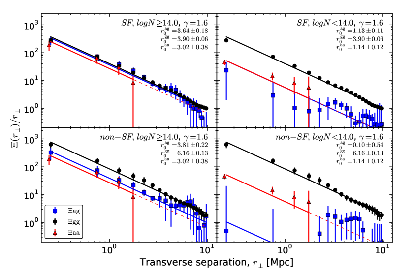
Figure 25: Same as Figure 23 but using a fixed slope, $\gamma=1.6$, for the power-law fits. These fits are for illustrative purposes only (see Section 7.2.6 for further details). Note that points and uncertainties are both correlated, and that uncertainties smaller than the symbols are not shown.

7.2.6 Results assuming a fixed slope $\gamma=1.6$

As mentioned in Section 6.4, if we assume that H i and galaxies do trace the same underlying dark matter distribution linearly, then we can use the different correlation lengths to obtain the relative linear biases between populations (e.g. Mo, Peacock & Xia, 1993; Ryan-Weber, 2006). For this method to work, we require the slopes of the correlation functions to be the same. Even though we have shown that this assumption is not always valid (at a $>3\sigma$ c.l.), in this section we fix the slope of the real-space correlations and repeat the analysis. We do this for illustrative purposes, so these results should not be taken as conclusive.

Figure 25 is the same as Figure 23, but using a fixed slope of $\gamma=1.6$. Judging from the plots, the fits work reasonably well for the galaxy–galaxy auto-correlations and the H i–galaxy cross-correlations for the ‘strong’ H i systems, but they fail to represent the H i–H i auto-correlations and the ‘weak’ H i–galaxy cross-correlations. These are expected results given what we observed in the previous analysis.

The top left panel of Figure 25 shows the results for our samples of ‘strong’ H i systems and ‘SF’ galaxies. We see that the $\xi_{\rm ag}(r)$ has a correlation length of $r_{0}^{\rm ag}=3.6\pm 0.2$  Mpc, whereas $\xi_{\rm gg}(r)$ and $\xi_{\rm aa}(r)$ have correlation lengths of $r_{0}^{\rm gg}=3.9\pm 0.1$  Mpc and $r_{0}^{\rm aa}=3.0\pm 0.4$  Mpc respectively. All these correlation lengths are consistent with each other within the uncertainties, indicating that ‘strong’ H i systems and ‘SF’ galaxies trace the same underlying dark matter distribution linearly. In fact, the ratio $(\xi_{\rm ag})^{2}/(\xi_{\rm gg}\xi_{\rm aa})\approx 1.1\pm 0.2$. From Equation 23 we have that the relative linear biases should be,

$$\begin{split}\left(\frac{b_{\rm g}}{b_{\rm a}}\right)=\left(\frac{r_{0}^{\rm gg}}{r_{0}^{\rm aa}}\right)^{\frac{\gamma}{2}}=\left(\frac{r_{0}^{\rm gg}}{r_{0}^{\rm ag}}\right)^{\gamma}\rm{,}\\ \end{split}$$ (28)

where $b_{\rm g}$ and $b_{\rm a}$ are the ‘SF’ and ‘strong’ H i biases respectively. Replacing the correlation lengths, we get that $b_{\rm g}:b_{\rm a}\sim 1.1-1.2$, which implies these objects belong to dark matter haloes of similar masses.

The bottom left panel of Figure 25 shows the results for our samples of ‘strong’ H i systems and ‘non-SF’ galaxies. We see that $\xi_{\rm ag}(r)$ has a correlation length of $r_{0}^{\rm ag}=3.8\pm 0.2$  Mpc, whereas $\xi_{\rm gg}(r)$ has a correlation length of $r_{0}^{\rm gg}=6.2\pm 0.1$  Mpc. The correlation length for $\xi_{\rm aa}(r)$ is the same as before. In contrast to the ‘SF’ case, the correlation length of ‘non-SF’ galaxies with themselves is significantly larger ($>3\sigma$ c.l.). In this case, the ratio $(\xi_{\rm ag})^{2}/(\xi_{\rm gg}\xi_{\rm aa})\approx 0.8\pm 0.1$. Consequently, LABEL:eq:biases2 is at the limit of its validity. Applying this equation, we find that $b_{\rm g}:b_{\rm a}\sim 1.8-2.2$.

The top right panel of Figure 25 shows the results for our samples of ‘weak’ H i systems and ‘SF’ galaxies. We see that $\xi_{\rm ag}(r)$ has a correlation length of $r_{0}^{\rm ag}=1.1\pm 0.1$  Mpc, and $\xi_{\rm aa}(r)$ also has $r_{0}^{\rm aa}=1.1\pm 0.1$  Mpc. The correlation length for $\xi_{\rm gg}(r)$ is the same as previously mentioned (two paragraphs above). In this case, the ratio $(\xi_{\rm ag})^{2}/(\xi_{\rm gg}\xi_{\rm aa})\approx 0.3\pm 0.1$. Consequently, LABEL:eq:biases2 should not hold. Still, if we apply this equation anyway, we find that $b_{\rm g}:b_{\rm a}\sim 2.6-7.6$.

The bottom right panel of Figure 25 shows the results for our samples of ‘weak’ H i systems and ‘non-SF’ galaxies. We see that $\xi_{\rm ag}(r)$ has a correlation length of $r_{0}^{\rm ag}=0.1\pm 0.5$  Mpc. The parameters for $\xi_{\rm aa}(r)$ and $\xi_{\rm gg}(r)$ are the same as previously mentioned (one and two paragraphs above respectively). In this case, the ratio $(\xi_{\rm ag})^{2}/(\xi_{\rm gg}\xi_{\rm aa})\approx 0.0\pm 0.1$. Consequently, LABEL:eq:biases2 should not hold either. Still, if we apply this equation, we find that $b_{\rm g}:b_{\rm a}\sim 4-700$.

7.3 Consistency checks

In order to check whether our results are robust, we have repeated the analysis using only H i systems and galaxies in their respective ‘a’ categories (i.e., best quality; see Sections 3.1.6 and 4.3). We found qualitative agreement with all our previous results, but a systematic increase in the correlation amplitudes by $\lesssim 10\%$ (with larger statistical uncertainties) was observed. Such a difference is expected due to the presence of random contamination in our ‘Full Sample’ (e.g. catastrophic failures, missidentification of H i systems, etc.). Still, within the uncertainties, the results from both analyses are fully consistent.

We also checked the effect of the Gaussian smoothing by repeating the analysis without smoothing at all (but still using the same linear grid). As expected, the new results for $r_{0}$ and $\gamma$ had increased statistical uncertainties but were all consistent with our previously reported values. We note that the slopes obtained from this new analysis were systematically larger by $\sim 10\%$ in most of the cases, but a $\sim 30\%$ increase was found for $\gamma^{\rm aa}$ and $\gamma^{\rm ag}$ in samples involving ‘weak’ H i systems.

8 Discussion

8.1 Comparison with previous results

In this section we compare our results with those published in other recent studies considering the H i–galaxy two-point correlation function at $z\lesssim 1$.

8.1.1 Comparison with Ryan-Weber (2006) results ($z\sim 0$)

Ryan-Weber (2006) measured the H i–galaxy cross-correlation at $z<0.04$ using H i data from the literature (Impey, Petry & Flint, 1999; Penton, Shull & Stocke, 2000; Bowen, Pettini & Blades, 2002; Penton, Stocke & Shull, 2004; Williger et al., 2006) and galaxy data from the H i Parkes All Sky Survey (HIPASS) (Doyle et al., 2005). Their total sample comprised $129$ H i absorption systems with $10^{12.5}\lesssim N_{\rm HI}\lesssim 10^{15}$  cm^-2, from $27$ QSO LOS; and $5317$ gas-rich galaxies.

Our results are in contrast with theirs. First, they found a strong ‘finger-of-god’ signal in the two-dimensional H i–galaxy cross-correlation, extending up to $\sim 10$  $h^{-1}_{100}$Mpc (see their figure 3), corresponding to an ‘anisotropy ratio’ of $\sim 10:1$. This anisotropy signal is also larger than they observed for the galaxy–galaxy auto-correlation, see their figure 2), meaning that it can not be explained by the galaxy redshift uncertainties. This result is in contrast to ours in that we do not see such a significant ‘finger-of-god’ signal, and the only anisotropy that we observe is consistent with being due to the galaxy redshift uncertainty.

Another difference between our results and theirs is the correlation length of the real-space correlations. They found $r_{0}^{\rm ag}=7.2\pm 1.4$  $h^{-1}_{100}$Mpc (which in our adopted cosmology corresponds to $r_{0}^{\rm ag}\approx 10.3\pm 2.0$  $h^{-1}_{70}$Mpc) imposing $\gamma^{\rm ag}$ to be equal to that of the $\xi_{\rm gg}(r)$, $\gamma^{\rm ag}\equiv\gamma^{\rm gg}=1.9\pm 0.3$. Although the slope is marginally consistent with what we find (see Section 7.2), the correlation length is more than $3\sigma$ c.l. larger than any of our values. If we set the slope of our correlations to be $\gamma=1.9$, we do not find consistency either (also note that a power-law fit for such a slope is not a good representation of our data). Ryan-Weber (2006) used this result to rule out ‘mini-haloes’ for the confinement of H i absorption systems. In view of our new results, we consider that this conclusion must be revisited (see Section 8.2.6).

Another intriguing result from Ryan-Weber (2006) is the fact that the amplitude of $\xi_{\rm ag}(r)$ is greater than that of $\xi_{\rm gg}(r)$. They found a $\xi_{\rm gg}(r)$ correlation length of $r_{0}^{\rm gg}=3.5\pm 0.7$  $h^{-1}_{100}$Mpc ($\approx 5.0\pm 1.0$  $h^{-1}_{70}$Mpc), which is somewhat larger but marginally consistent with our findings. In order to explain the larger $r_{0}^{\rm ag}$ value with respect to $r_{0}^{\rm gg}$, $\xi_{\rm aa}(r)$ should be greater than both $\xi_{\rm gg}(r)$ and $\xi_{\rm ag}(r)$. This hypothesis is difficult to understand within the current cosmological paradigm, and in fact, it is not supported by our results on the H i–H i auto-correlation either.

We note that the surveys have important differences, in particular regarding the galaxy samples. HIPASS selected galaxies based on H i emission, i.e. containing significant amounts of neutral gas. It also includes low-surface brightness galaxies that might be lacking in ours. The clustering of these galaxies is expected to be lower than that of brighter galaxies in our sample though, which goes in the opposite direction of what is needed to reconcile our results with those of Ryan-Weber (2006). The much lower redshift range in their sample might also have an impact on the clustering, as structures are more collapsed. This might help to increase the correlation lengths, but it should not make the $\xi_{\rm ag}(r)$ amplitude greater than $\xi_{\rm gg}(r)$ by itself. Another possibility is that this might be a case in which the ratio $(\xi_{\rm ag})^{2}/(\xi_{\rm gg}\xi_{\rm aa})>1$, meaning that the H i and galaxies observed actually correspond to the same physical objects (see Section 6.4). Such an effect should be most noticeable at the smallest scales, but this is not supported by their results. Indeed, there is a flattening in their reported $\Xi_{\rm ag}(r_{\perp})/r_{\perp}$ at $\lesssim 1$  $h^{-1}_{100}$Mpc (see their figure 5) which makes the H i–galaxy cross-correlation consistent with the galaxy–galaxy auto-correlation at these scales.

8.1.2 Comparison with Wilman et al. (2007) results ($z\lesssim 1$)

Wilman et al. (2007) measured the H i–galaxy cross-correlation at $z\lesssim 1$ using data from Morris & Jannuzi (2006). Their total sample comprised $381$ H i absorption systems with $10^{13}\lesssim N_{\rm HI}\lesssim 10^{19}$  cm^-2, from $16$ QSO LOS; and $685$ galaxies at $\lesssim 2$  $h^{-1}_{100}$Mpc from the QSO LOS, of which, $225$ were classified as ‘absorption-line-dominated’ and $406$ as ‘emission-line-dominated’.

We find qualitative agreement with their observational results in the following sense: (i) no strong ‘finger-of-god’ effect is seen in the observed H i–galaxy cross-correlation; (ii) the larger the $N_{\rm HI}$, the stronger the clustering with galaxies; and (iii) no evidence that ‘emission-line-dominated’ galaxies cluster more strongly with H i systems than ‘absorption-line-dominated’ ones (in contrast to what was reported by Chen & Mulchaey, 2009, see below).

Wilman et al. (2007) also performed a comparison with a cosmological hydrodynamical simulation. In contrast to their observational results, they did find a strong ‘finger-of-god’ effect (similar to that found by Ryan-Weber, 2006) in their simulated data (see their figure 6). This prediction is in not supported by our observations, as we do not detect such a strong anisotropy feature.

8.1.3 Comparison with Pierleoni, Branchini & Viel (2008) results (simulations)

Pierleoni, Branchini & Viel (2008) investigated the observational results from Ryan-Weber (2006) and Wilman et al. (2007) in the context of a cosmological hydrodynamical simulation. They selected samples of simulated H i absorption systems and galaxies, trying to match those from Ryan-Weber (2006).

Contrary to the Ryan-Weber (2006) observational results (and the prediction from Wilman et al., 2007), they did not find a strong ‘finger-of-god’ signal in the mock H i–galaxy cross-correlation (see their figure 7), which agrees with our observational result. In contrast, they find a compression along the LOS at scales $\gtrsim 4$  $h^{-1}_{100}$Mpc, similar to the expectation from the ‘Kaiser effect’ (Kaiser, 1987). We did not detect such a feature but note that our survey was not designed to do so.

They also found that the peak in the two-dimensional H i–galaxy cross-correlation was offset along the LOS by about $\sim 1$  $h^{-1}_{100}$Mpc. A similar signal was observed in our sample of ‘strong’ H i systems and ‘non-SF’ galaxies (see Figure 19), but these two results are not directly comparable. Indeed, we do not observe such a feature in our ‘Full Sample’. Still, we caution the reader that a $\sim 1$  $h^{-1}_{100}$Mpc displacement in the LOS direction is comparable to our galaxy redshift uncertainty ($\sim 1.4-1.7$  $h^{-1}_{70}$Mpc), and so such a signal might get easily diluted.

Another qualitative agreement between our results and those from Pierleoni, Branchini & Viel (2008) is that the amplitude of the H i–galaxy cross-correlation is smaller than that of the galaxy–galaxy auto-correlation, and that the H i–H i auto-correlation is smaller still (see their figures 3 and 9). Quantitatively, they found that $\xi_{\rm ag}(r)$ and $\xi_{\rm gg}(r)$ have correlation lengths of $r_{0}^{\rm ag}=1.4\pm 0.1$  $h^{-1}_{100}$Mpc ($\approx 2.0\pm 0.1$  $h^{-1}_{70}$Mpc) and $r_{0}^{\rm gg}=3.1\pm 0.2$  $h^{-1}_{100}$Mpc ($\approx 4.4\pm 0.2$  $h^{-1}_{70}$Mpc), and slopes $\gamma^{\rm ag}=1.29\pm 0.03$ and $\gamma^{\rm gg}=1.46\pm 0.03$ respectively. These values are marginally consistent with our findings (see Table 8). Moreover, they predict a flattening of $\xi_{\rm aa}(r)$ at scales $\lesssim 1$  $h^{-1}_{100}$Mpc, which is also consistent with our observations.

Finally, we also find agreement in the sense that the amplitude of the H i–galaxy cross-correlation significantly increases for high column density absorbers, but little variation is observed for different galaxy samples selected by mass (see their figure 4). Even though we do not have direct measurements of galaxy masses in our galaxy samples, the significantly larger auto-correlation amplitude of ‘non-SF’ galaxies with respect to ‘SF’ suggests that, on average, ‘non-SF’ galaxies typically belong to more massive dark matter haloes than ‘SF’ galaxies (see also Section 8.2.6).

8.1.4 Comparison with Chen & Mulchaey (2009) results ($z\lesssim 0.5$)

Chen & Mulchaey (2009) measured the H i–galaxy cross-correlation at $z\lesssim 0.5$ from their own H i and galaxy survey (including data from Chen et al., 2005). Their total sample comprised $195$ H i absorption systems with $10^{12.5}\lesssim N_{\rm HI}\lesssim 10^{16}$  cm^-2, from $3$ QSO LOS; and $670$ galaxies at $\lesssim 4$  $h^{-1}_{100}$Mpc from the QSO LOS, of which $222$ are classified as ‘absorption-line-dominated’ and $448$ as ‘emission-line-dominated’.

In this case, we find both agreements and disagreements. Our results agree with theirs in the sense that the clustering of ‘strong’ H i systems ($N_{\rm HI}\geq 10^{14}$  cm^-2) with galaxies is stronger than that of ‘weak’ H i systems and galaxies (see their figure 13), and that ‘strong’ H i systems and ‘emission-line-dominated’ galaxies have comparable clustering amplitudes. However, our results disagree with their claim that ‘strong’ H i systems cluster more strongly with ‘emission-line-dominated’ than with ‘absorption-line-dominated’ (see their figure 13). In fact, our findings are consistent with the amplitude of the H i–galaxy cross-correlation being independent of spectral type (within the statistical uncertainties). Moreover, we find that the H i–galaxy cross-correlation for ‘non-SF’ galaxies is systematically stronger than that of ‘SF’ galaxies, which is the opposite to what Chen & Mulchaey (2009) found.

Quantitatively, they reported a $\sim 6\times$ smaller clustering amplitude between ‘strong’ H i absorption systems and ‘SF’ galaxies than that of ‘non-SF’ galaxies with themselves, whereas we find this difference to be a factor of $\sim 2$ only. We note that their quoted statistical errors are Poissonian, which underestimate the true uncertainties. The Poissonian uncertainty in our survey is typically $\sim 1$ order of magnitude smaller than our adopted ‘bootstrap’ one (see Section 6.5). Thus, there is still room for their results to agree with ours after taking this fact into account. There is also the possibility that sample/cosmic variance is significantly affecting their results. We note that one of the three QSO LOS used by them passes at $\sim 2$  Mpc from the Virgo Cluster. Even though this single cluster is not likely to explain the discrepancy, any sightline passing through it is also probing an unusually high overdensity in the local Universe (which extends beyond the Virgo Cluster itself).

8.1.5 Comparison with Shone et al. (2010) results ($z\sim 1$)

Shone et al. (2010) measured the H i–galaxy cross-correlation at $0.7\lesssim z\lesssim 1.5$ from their own H i and galaxy survey. Their total sample comprised $586$ H i absorption systems with $10^{13.2}\lesssim N_{\rm HI}\lesssim 10^{17}$  cm^-2, from $2$ QSO LOS; and $193$ galaxies at $\lesssim 4$  $h^{-1}_{70}$Mpc from the QSO LOS ($196$ absorber–galaxy pairs used).

They found the peak in the two-dimensional H i–galaxy cross-correlation to be $\xi_{\rm ag}^{\rm peak}=1.9\pm 0.6$ (although displaced from the smallest separation bin by $\sim 5$  $h^{-1}_{70}$Mpc along the LOS; see their figure 12), whereas $\xi_{\rm gg}^{\rm peak}=10.7\pm 1.4$ for the galaxy–galaxy auto-correlation (see their figure 13). Our results agree with theirs qualitatively in the sense that the clustering of H i and galaxies is weaker than that of the galaxies with themselves.

8.1.6 Summary

In summary, we have found agreements and disagreements with previously published results. We consider the majority of the discrepancies to be driven by the inherent difficulty of addressing uncertainties in this type of analysis, which often lead to an underestimation of the errors.

8.2 Interpretation of the results

In this section we provide our preferred interpretation of our observational results.

8.2.1 Probabilistic interpretation (model independent)

The clustering analysis provides an essentially model independent statistic. The amplitude of the two-point correlation function corresponds to the probability excess of finding a pair compared to the Poissonian expectation. Thus, our results point towards the following conclusions:

• The probability of finding a ‘SF’ galaxy at a distance $\lesssim 5$  Mpc from another ‘SF’ galaxy, is $\sim 2\times$ smaller than that of finding a ‘non-SF’ galaxy at that same distance from another ‘non-SF’ galaxy.

• The probability of finding a H i absorption system with $N_{\rm HI}\geq 10^{14}$  cm^-2 at a distance $\lesssim 5$  Mpc from a ‘SF’ galaxy, is approximately the same as that of finding a ‘SF’ galaxy at that same distance from another ‘SF’ galaxy.

• The probability of finding a H i absorption system with $N_{\rm HI}<10^{14}$  cm^-2 at a distance $\lesssim 5$  Mpc from a ‘SF’ galaxy, is $\sim 10\times$ smaller than that of finding a ‘SF’ galaxy at that same distance from another ‘SF’ galaxy.

• The probability of finding a H i absorption system with $N_{\rm HI}\geq 10^{14}$  cm^-2 at a distance $\lesssim 5$  Mpc from a ‘non-SF’ galaxy, is $\sim 2\times$ smaller than that of finding a ‘non-SF’ galaxy at that same distance from another ‘non-SF’ galaxy.

• The probability of finding a H i absorption system with $N_{\rm HI}<10^{14}$  cm^-2 at a distance $\lesssim 5$  Mpc from a ‘non-SF’ galaxy, is $\gtrsim 100\times$ smaller than that of finding a ‘non-SF’ galaxy at that same distance from another ‘non-SF’ galaxy.

• The probability of finding a H i absorption system with $N_{\rm HI}<10^{14}$  cm^-2 at a distance $\lesssim 2$  Mpc from another $N_{\rm HI}<10^{14}$  cm^-2 system is $\sim 4\times$ smaller than that of finding a $N_{\rm HI}\geq 10^{14}$  cm^-2 system at that same distance from another $N_{\rm HI}\geq 10^{14}$  cm^-2 system.

Any physical model aiming to explain the connection between H i absorption systems and galaxies at $z\lesssim 1$ will need to take these constraints into account.

8.2.2 Velocity dispersion between H i and galaxies

We find that the two-dimensional H i–galaxy cross-correlations do not show detectable velocity distortions along the LOS larger than those expected from the galaxy redshift uncertainties. As mentioned, the typical uncertainty for our single galaxy redshift determination is $\Delta z_{\rm gal}\approx 0.0006/\sqrt{2}$, which is equivalent to rest-frame velocity differences of $\Delta v\sim 120-60$ at $z=0.1-1$, respectively. Any velocity dispersion between H i systems and galaxies greater than, or of the order of, this value, would have been noticeable in the two-dimensional H i–galaxy cross-correlation signals. Therefore, we conclude that the bulk of H i systems on $\sim$ Mpc scales, have little velocity dispersion ($\lesssim 120$ ) with respect to the bulk of galaxies. Hence, no strong galaxy outflow or inflow signal is detected in our data.

We emphasize that our results are based on H i only. Given that H i does not exclusively trace gas originating in galaxy outflows or inflows, we do not necessarily expect to find the same signatures as those traced by metals. Moreover, our results are dominated by scales somewhat larger than those typically associated to the CGM, in which the outflow or inflow signal is expected to be maximized. In view of these considerations, it is not surprising that no strong outflow or inflow signal is detected in our data.

We also emphasize that the cross-correlation analysis provides an averaged statistical result; individual galaxies having strong H i inflows/outflows might still be present, but our results indicate that these do not dominate the cross-correlation signal at $z\lesssim 1$.

8.2.3 Spatial distribution of H i and galaxies

The absolute and relative clustering amplitudes of our different populations of H i and galaxies can be used to give us an idea of their spatial distribution. Our conclusions on this are as follows:

• The fact that ‘strong’ H i systems and ‘SF’ galaxies have similar amplitudes and slopes for the auto- and cross-correlation, indicates that these are distributed roughly in the same locations.

• The fact that the auto-correlation of ‘non-SF’ has also the same slope but a larger amplitude, indicates that there are sub-locations (within those where galaxies and ‘strong’ H i systems reside) with a higher density of ‘non-SF’ galaxies than ‘SF’ galaxies and/or ‘strong’ H i systems. This interpretation also explains the fact that the ratio $(\xi_{\rm ag})^{2}/\xi_{\rm gg}\xi_{\rm aa}$ for ‘strong’ H i systems and ‘non-SF’ galaxies is consistent with neither $1$ nor $0$ (see Section 8.2.4).

• The suggestion that the self-clustering of ‘weak’ systems is not zero, and the fact that ‘weak’ H i systems and galaxies have a ratio $(\xi_{\rm ag})^{2}/\xi_{\rm gg}\xi_{\rm aa}\approx 0$, indicate that these are not distributed in the same locations. Therefore, there are locations containing ‘weak’ H i systems but roughly devoid of ‘strong’ H i systems and galaxies of any kind.

This picture fits well with the recent results presented in Tejos et al. (2012), from their study of the distribution of H i absorption systems within and around galaxy voids at $z\lesssim 0.1$. They showed that galaxy voids are not empty, and in fact contain about $\sim 20-40\%$ of H i absorption line systems with $N_{\rm HI}\gtrsim 10^{12.5}$  cm^-2. The remaining $\sim 60-80\%$ were found at the edges of galaxy voids, hence sharing locations with galaxies.

Even though it seems natural to identify our ‘weak’ systems with those systems found in galaxy voids, not all ‘weak’ systems need to be unassociated with galaxies. Despite the fact that Tejos et al. (2012) reported a (tentative) difference in the column density distributions between H i absorbers within and around galaxy voids (at the $\sim 2\sigma$ c.l.), they did not find sharp $N_{\rm HI}$ transitions between their samples. The most important difference came from the presence of ‘extremely weak’ H i systems, $N_{\rm HI}\lesssim 10^{13}$  cm^-2, that were present within galaxy voids but not outside (see their figures 2 and 3). Such a low column density is at the limit of our current completeness (see Section 4.5) and so we are not able to give confident results on the clustering of these ‘extremely weak’ H i systems either with themselves or with galaxies. Restricting the column density range to $10^{13}\leq N_{\rm HI}<10^{14}$  cm^-2, there are $19/50\sim 40\%$ systems within galaxy voids in the Tejos et al. (2012) sample. In the following we will estimate the fraction of ‘weak’ systems that could still be associated with galaxies in our current sample.

It is straightforward to show that the two-point correlation function between two populations, $a$ and $b$, each one composed by sub-populations $a_{i}$ where $i\in\{0,1,...,N_{a}\}$, and $b_{j}$ where $j\in\{0,1,...,N_{b}\}$, respectively, is

$$\xi_{ab}=\sum_{i}^{N_{a}}\sum_{j}^{N_{b}}f_{i}f_{j}\xi_{a_{i}b_{j}}\ \rm{,}$$ (29)

where $\xi_{a_{i}b_{j}}$ is the cross-correlation between the $a_{i}$ and $b_{j}$ sub-populations (assumed positive), and $f_{i}$ and $f_{j}$ are the fractions of $a_{i}$ and $b_{j}$ objects over the total samples $a$ and $b$, respectively. Thus, if we think of ‘weak’ absorbers being composed of two kinds of populations, we have,

$$\xi_{aa}^{\rm weak}=f_{a_{1}}^{2}\xi_{a_{1}a_{1}}+f_{a_{2}}^{2}\xi_{a_{2}a_{2}}+2f_{a_{1}}f_{a_{2}}\xi_{a_{1}a_{2}}\ \rm{.}$$ (30)

If we consider a scenario in which one of these populations clusters in the same way as ‘strong’ H i systems ($\xi_{a_{1}a_{1}}\equiv\xi_{aa}^{\rm strong}$) and the other is completely random ($\xi_{a_{2}a_{2}}=\xi_{a_{1}a_{2}}\equiv 0$), then,

$$\xi_{aa}^{\rm weak}=f_{a_{1}}^{2}\xi_{aa}^{\rm strong}\ \rm{,}$$ (31)

From this, we can estimate the fraction of ‘weak’ systems that could be clustered like ‘strong’ ones as $f_{a_{1}}=\sqrt{\xi_{aa}^{\rm weak}/\xi_{aa}^{\rm strong}}\sim 0.5$. We note that the assumption that one of the sub-populations has $\xi_{a_{2}a_{2}}\equiv 0$ might be unrealistic, because $\xi_{aa}^{\rm weak}$ and $\xi_{aa}^{\rm strong}$ have marginally different slopes, and a random component does not change the slope but only the amplitude of the correlation function. Also, if both populations lie exclusively in different locations, the cross-correlation should be $\xi_{a_{1}a_{2}}<0$, which makes $\xi_{a_{1}a_{2}}\equiv 0$ unrealistic too. These two effects go in opposite directions for the final fraction estimation however, which might in the end compensate each other. With this caveat in mind, this rough estimation seems consistent with what Tejos et al. (2012) found for systems in the range $10^{13}\lesssim N_{\rm HI}\lesssim 10^{14}$  cm^-2 ($\sim 60\%$; see above).

8.2.4 H i and non-star-forming galaxies

Our results point towards ‘strong’ H i systems and ‘non-SF’ galaxies having a ratio $(\Xi_{\rm ag})^{2}/(\Xi_{\rm gg}\Xi_{\rm aa})\approx 0.5\pm 0.3$, which is consistent with neither $1$ nor $0$ at the $\sim 1\sigma$ c.l.. In order to explain this result we will consider the presence of two types of ‘non-SF’ galaxies: one type ($g_{1}$) that correlates linearly with ‘strong’ H i absorbers, and another type ($g_{2}$) that does not. Thus,

$$\begin{split}\frac{(\xi_{ag_{1}})^{2}}{(\xi_{aa})(\xi_{g_{1}g_{1}})}&\equiv 1\ \rm{,}\\ \frac{(\xi_{ag_{2}})^{2}}{(\xi_{aa})(\xi_{g_{2}g_{2}})}&\equiv 0\ \rm{.}\\ \end{split}$$ (32)

Let $f_{g_{1}}$ and $f_{g_{2}}$ be the fraction of ‘non-SF’ galaxies of type $g_{1}$ and $g_{2}$, respectively, such that $f_{g_{1}}+f_{g_{2}}=1$. Then, from Equation 29 we have,

$$\begin{split}\xi_{ag}&=f_{g_{1}}\xi_{ag_{1}}+f_{g_{2}}\xi_{ag_{2}}\\ &=f_{g_{1}}\xi_{ag_{1}}\ \rm{,}\\ \end{split}$$ (33)

because $\xi_{ag_{2}}=0$. Similarly,

$$\begin{split}\xi_{gg}&=f_{g_{1}}^{2}\xi_{g_{1}g_{1}}+f_{g_{2}}^{2}\xi_{g_{2}g_{2}}+2f_{g_{1}}f_{g_{2}}\xi_{g_{1}g_{2}}\\ &=f_{g_{1}}^{2}\xi_{g_{1}g_{1}}+f_{g_{2}}^{2}\xi_{g_{2}g_{2}}\ \rm{,}\ \end{split}$$ (34)

because $\xi_{g_{1}g_{2}}\approx 0$ also. Our observational results indicate that,

$$\begin{split}\frac{(\xi_{ag})^{2}}{(\xi_{aa})(\xi_{gg})}=\alpha\ \rm{,}\\ \end{split}$$ (35)

with $0<\alpha<1$. Combining these relations we find the following quadratic equation for $f_{g_{1}}$,

$$(1-\alpha-\alpha\beta)f_{g_{1}}^{2}+2\alpha\beta f_{g_{1}}-\alpha\beta=0\ \rm{.}$$ (36)

where $\beta\equiv\xi_{g_{2}g_{2}}/\xi_{g_{1}g_{1}}$. Solving Equation 36 for a positive solution smaller than $1$, gives us our estimation of the required fraction of ‘non-SF’ galaxies that are correlated with ‘strong’ H i systems linearly, for the given $(\xi_{ag})^{2}/(\xi_{aa})(\xi_{gg})$ and $\xi_{g_{2}g_{2}}/\xi_{g_{1}g_{1}}$ ratios.

Our proposed scenario aims to approximate what might be the case for galaxy clusters, which contain an important fraction of ‘non-SF’ galaxies but whose diffuse IGM or CGM can get destroyed by baryonic physics (e.g. Morris et al., 1993; Lopez et al., 2008; Padilla et al., 2009; Yoon et al., 2012). In such a case, $\xi_{g_{2}g_{2}}/\xi_{g_{1}g_{1}}\gg 1$ because galaxy clusters represent the most massive dark matter haloes. Measurements and predictions for the auto-correlation of galaxy clusters point towards correlation lengths of $r_{0}^{\rm cc}\sim 20-30$  Mpc (e.g. Colberg et al., 2000; Estrada, Sefusatti & Frieman, 2009; Hong et al., 2012), which would imply a $\xi_{g_{2}g_{2}}/\xi_{g_{1}g_{1}}\sim 10\pm 5$ (assuming a slope of $\gamma=1.6$). Using this value together with $(\xi_{ag})^{2}/(\xi_{aa})(\xi_{gg})=0.5\pm 0.3$, we find the fraction $f_{g_{1}}\approx 0.75\pm 0.15$ and consequently $f_{g_{2}}\approx 0.25\pm 0.15$.

Therefore, our results suggest that an important fraction of ‘non-SF’ galaxies ($\sim 60-90\%$) trace the same underlying dark matter distribution as ‘strong’ H i systems and ‘SF’ galaxies at scales $\lesssim 2$  Mpc. This is in contrast with what can be inferred from the results reported by Chen & Mulchaey (2009), in which ‘strong’ H i systems cluster more weakly with ‘non-SF’ than ‘SF’ galaxies (see Section 8.1.4). In such a case, $(\xi_{ag})^{2}/(\xi_{aa})(\xi_{gg})\approx 0$, implying a fraction close to $f_{g_{1}}\sim 0$.

Our simple interpretation agrees quite well with the recent observational results presented by Thom et al. (2012). These authors found that $11/15\sim 70\%$ of their sample of ‘non-star-forming-galaxies’ at low-$z$, have H i absorption with rest-frame equivalent widths, $W_{r}>0.3$ Å (equivalent to $\gtrsim 10^{14}$  cm^-2), within $300$ from their systemic redshifts, and at impact parameters $\lesssim 200$  kpc (see their figures 2 and 3). By definition, these H i systems should be associated with the CGM of these galaxies. However, because of incompleteness in the galaxy surveys, it is not certain that this gas is purely associated to these ‘non-star-forming-galaxies’ (less luminous ‘star-forming-galaxies’ could have been missed by their target selection; e.g. Stocke et al., 2013). Still, both Thom et al. (2012) and our results point towards the conclusion that a significant fraction of ‘non-star-forming-galaxies’ share locations with ‘strong’ H i systems at scales $\lesssim 2$  Mpc. Thus, our results indicate that the ‘cold gas’ (traced by ‘strong’ H i) around ‘non-SF’ galaxies could be the rule rather than the exception.

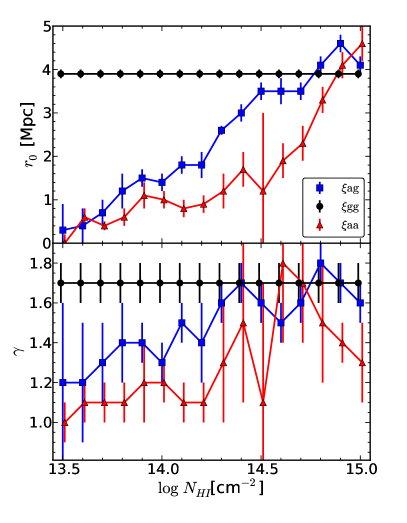
Figure 26: Correlation lengths (top panel) and slopes (bottom panel) from the best power-law fits of the ‘real-space’ correlation functions of the form presented in Equation 19, as a function of H i column density bins of $1$ dex width each, from which the correlation functions were measured. Different symbols/colors show our different measurements: the blue squares correspond to the galaxy-H i cross-correlation ($\xi_{\rm ag}$); the black circles to the galaxy-galaxy auto-correlation ($\xi_{\rm gg}$; slightly shifted along the $x$-axis for the sake of clarity); and the red triangles to the H i-H i auto-correlation ($\xi_{\rm aa}$; slightly shifted along the $x$-axis for the sake of clarity). Note that points associated with the galaxy auto-correlation are independent of H i column density. Note that points and uncertainties are both correlated.

8.2.5 Column density limit

Our choice of a $10^{14}$  cm^-2 limit was somewhat arbitrary (see Section 4.6). As mentioned, when we increase the limit for dividing ‘strong’ versus ‘weak’ systems from $10^{14}$ to $\sim 10^{15-16}$  cm^-2, we get larger cross-correlation amplitudes and slopes (although with larger uncertainties due to the reduced number of systems above such limits in our sample) for ‘strong’ compared to those from ‘weak’ systems. Similarly, when we decrease the limit from $10^{14}$ to $\sim 10^{13}$  cm^-2, we observe a decrease in the cross-correlation amplitudes and slopes of ‘strong’ systems. In this section we explore more on this issue.

In order to quantify the H i-galaxy cross-correlation dependence on H i column density, we have repeated the analysis using subsamples of the H i absorption systems based on $N_{\rm HI}$ limits, together with all galaxies in our ‘Full Sample’. We used $16$ $N_{\rm HI}$ bins of $1$ dex width each, shifted by $0.1$ dex, starting from $[10^{13},10^{14}]$ through $[10^{14.5},10^{15.5}]$  cm^-2. Figure 26 shows the correlation lengths (top panel) and slopes (bottom panel) from the best power-law fits of the ‘real-space’ correlation functions of the form presented in Equation 19, for each of those $N_{\rm HI}$ bins. Different symbols/colors show our different measurements: the blue squares correspond to the galaxy-H i cross-correlation ($\xi_{\rm ag}$); the black circles to the galaxy-galaxy auto-correlation ($\xi_{\rm gg}$; slightly shifted along the $x$-axis for the sake of clarity); and the red triangles to the H i-H i auto-correlation ($\xi_{\rm aa}$; slightly shifted along the $x$-axis for the sake of clarity). Note that points associated with the galaxy auto-correlation are independent of H i column density, and that points and uncertainties are both correlated. As expected, we see an overall monotonic increase in the correlation length and slopes with increasing $N_{\rm HI}$. Such a behaviour can be explained by assuming that the fraction of H i systems that are not correlated with galaxies decreases with an increase in the minimum column density limit. Any change in the amplitude of the correlation functions can be understood as a change in the ‘linear bias’ and/or the fraction of ‘random contamination’ present. Changes in the slope of the correlations (like the one we have marginally observed in this work) would require the addition of baryonic physics, assuming a fixed underlying dark matter slope. We also observe that the $\xi_{\rm ag}$ and $\xi_{\rm gg}$ have comparable amplitudes (within $2\sigma$) for column density bins centred at $10^{14.5}$  cm^-2 and above, which corresponds to $N_{\rm HI}\gtrsim 10^{14}$  cm^-2. As mentioned, this is one of the reasons that motivated our adopted limit of $10^{14}$  cm^-2 for splitting our H i sample (see Section 4.6).

These results show that there is a dramatic change in the H i-galaxy cross-correlation signal, where the correlation length changes from being consistent with $0$  Mpc at $N_{\rm HI}$ $\in[10^{13},10^{14}]$  cm^-2, to being consistent with the $\xi_{\rm gg}$ value of $\sim 4$  Mpc at $N_{\rm HI}$ $\in[10^{14},10^{15}]$  cm^-2. The slope of the H i–galaxy cross-correlation also follows the same trend. This is an important change occurring in about one order of magnitude column density range. Given the $1$ dex binning used for this analysis (needed to reduce the statistical uncertainties), we cannot rule out an even sharper transition occurring within the $\sim 10^{13}-10^{14}$  cm^-2 range with our current data.

Recent theoretical results also suggest that a $10^{14}$  cm^-2 limit might have a physical meaning. Davé et al. (2010) used a cosmological hydrodynamical simulation to study the properties of H i absorption systems from $z=2$ to $z=0$. They found an interesting bimodality in the distribution of $\log N_{\rm HI}$ per unit path length at $\langle z\rangle\approx 0.25$, where $N_{\rm HI}<10^{14}$  cm^-2 systems are dominated by the diffuse IGM and $N_{\rm HI}>10^{14}$  cm^-2 are dominated by the condensed IGM associated with galaxy halos (see their figure 10). This theoretical result is supported by our observations of the similar clustering amplitudes of all $\xi_{\rm ag}$, $\xi_{\rm aa}$ and $\xi_{\rm gg}$ albeit at a somewhat larger limit of $N_{\rm HI}\sim 10^{14.5}$  cm^-2 (see Figure 26).

According to the results from Davé et al. (2010), the diffuse IGM approximately follows,

$$\frac{\rho}{\bar{\rho}}\approx 50\left(\frac{N_{\rm HI}}{10^{14}\,{\rm cm}^{-2}}\right)^{0.74}10^{-0.37z}\rm{,}$$ (37)

where $\rho/\bar{\rho}$ is the local baryonic density in units of the cosmic mean (see their equation 3 and figure 9). This gives us an idea of the overdensities involved (see also Schaye, 2001, for a similar relationship from analytical arguments). A change of one order of magnitude in column density corresponds to a factor of $\sim 5$ (directly proportional) in $\rho/\bar{\rho}$, whereas a change of one unit redshift corresponds to a factor of $\sim 2$ (inversely proportional) in $\rho/\bar{\rho}$. Thus, a limit of $10^{14}$  cm^-2 would correspond to overdensities of $\sim 50\times$ and $\sim 25\times$ the cosmic mean at $z=0$ and $z=1$, respectively. Similarly, limits of $10^{13}$ and $10^{15}$  cm^-2 would correspond to $\sim 5\times$ more and less than those values, respectively. We emphasize that there are large scatters involved in this relation: roughly one order of magnitude in overdensity for a fixed H i column density, and roughly half an order of magnitude in H i column density for a fixed overdensity. Such a scatter would likely end up diluting any sharper $N_{\rm HI}$ transition.

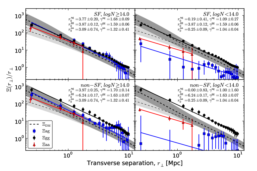
Figure 27: Same as Figure 23 with the prediction for the dark matter clustering at $z\lesssim 1$ (dashed line). The shaded regions enclose the expected dark matter clustering between redshift $z=1$ (lower envelope) and $z=0$ (upper envelope) while the dashed lines themselves correspond to the expectation at $z=0.5$. These predictions were obtained from the dark matter power spectrum provided by camb (Lewis, Challinor & Lasenby, 2000), with (thick dashed lines and dark shaded regions) and without (thin dashed lines and light shaded regions) using the non-linear corrections of Smith et al. (2003), for our adopted cosmological parameters and $\sigma_{8}=0.8$. See Section 8.2.6 for further details.

8.2.6 Dark matter halo masses hosting H i systems and galaxies

It is common practice to compare the observed clustering amplitudes of extragalactic objects (e.g. galaxies, galaxy clusters, IGM absorbers, etc.) with that of the expected theoretical (cold) dark matter in a given cosmological framework, in order to infer a typical dark matter halo mass for the confinement of such objects (e.g. Mo, Peacock & Xia, 1993; Ryan-Weber, 2006). This method is model dependent, and it is only applicable over narrow cosmological epochs (narrow redshift ranges).

Our sample is composed of objects at $0\lesssim z\lesssim 1$, which corresponds to about half of the history of the Universe. Thus, a direct link between the clustering amplitudes reported in this paper with a single dark matter halo mass is not meaningful. Still, simple reasoning leads to the conclusion that the typical dark matter haloes for the confinement of H i systems and galaxies, should follow the same trends as the amplitudes of their correlation functions. Therefore, the most massive ones should correspond to ‘non-SF’ galaxies, followed by ‘SF’ galaxies, ‘strong’ H i systems (both comparable) and ‘weak’ H i systems, in that same order.

Figure 27 is the same as Figure 23 but including the prediction for the dark matter clustering at $z\lesssim 1$ (thick dashed line). The shaded regions enclose the expected dark matter clustering between redshift $z=1$ (lower envelope) and $z=0$ (upper envelope), while the dashed lines correspond to the expectation at $z=0.5$. These predictions were obtained from the dark matter power spectrum provided by camb (Lewis, Challinor & Lasenby, 2000), with (thick dashed lines and dark shaded regions) and without (thin dashed lines and light shaded regions) the non-linear corrections of Smith et al. (2003), for our adopted cosmological parameters and $\sigma_{8}=0.8$. We see that the shape of the correlations for ‘strong’ H i systems and galaxies are approximately consistent with that of the predicted dark matter in the non-linear regime. Their somewhat larger amplitudes hint towards ‘absolute biases’ $b\gtrsim 1$. On the other hand, the shape of the ‘weak’ H i is marginally in disagreement with that of the dark matter expectation in the non-linear regime. In this case, the lower amplitude compared to that of the dark matter hints towards an ‘absolute bias’ $b<1$. We note that for the case of ‘weak’ systems, a linear approximation for the dark matter clustering (i.e. neglecting the correction of Smith et al., 2003), gives a somewhat better match in terms of slopes, although still with amplitudes marginally above our observed ones. If a significant fraction of ‘weak’ H i systems reside in underdense regions (i.e. within galaxy voids), a linear evolution should be expected even at $z\approx 0$. We speculate that H i systems within galaxy voids are still evolving in the linear regime, even at scales $\lesssim 2$  Mpc.

In view of these results, we revisit the claim by Ryan-Weber (2006) that H i absorption systems with $\lesssim 10^{15}$  cm^-2 reside preferentially in dark matter halo of masses $M\sim 10^{13.6}-10^{14.5}$ $h^{-1}_{100}$M_☉, analogous to those of massive galaxy groups. Given the significantly lower clustering amplitude of our full sample of H i systems compared to that of galaxies, we conclude that H i absorption systems are preferentially found in dark matter haloes of masses smaller than those populated by galaxies. At most, ‘SF’ galaxies and ‘strong’ H i systems are typically found in dark matter haloes of similar masses. Moreover, a significant fraction of ‘weak’ H i systems might reside in underdense regions with ‘absolute biases’ $b<1$.

8.2.7 Three types of relationships between H i and galaxies

We have reported a significant ($>3\sigma$ c.l.) rejection of the hypothesis that H i absorption systems and galaxies (as a whole) trace the same underlying dark matter distribution linearly (see Section 7). We have found that this is mostly driven by H i absorption systems with column densities $N_{\rm HI}<10^{14}$  cm^-2 (‘weak’ systems), which show little (consistent with $0$) correlation with galaxies. On the other hand, H i systems with $N_{\rm HI}\geq 10^{14}$  cm^-2 (‘strong’ systems) are consistent with such an hypothesis. Thus, this indicates the presence of, at least, two types of relationships between H i and galaxies: (i) linear correlation, and (ii) no correlation.

A third type of relationship comes from the fact that at small enough scales, H i systems and galaxies are a different manifestation of the same physical object; a galaxy is also a very strong H i absorption system and, depending on the galaxy definition, the other way around also applies. Our survey was not designed for studying scales $\lesssim 0.5$  Mpc, and so it is not surprising that we do not observe a characteristic signal of a one-to-one association (see Section 6.4). Thus, we can not neglect the fact that this relationship exists and should be included in our interpretation. Still, the contribution of this one-to-one correlation between H i absorption systems and luminous galaxies to the total fraction of H i systems at $10^{13}\lesssim N_{\rm HI}\lesssim 10^{17}$  cm^-2 is quite low.

This picture fits well with what was presented early by Mo & Morris (1994b), and is in contrast to the commonly adopted interpretation presented by Lanzetta et al. (1995) which claims that the majority of low-$z$ H i systems belong to the extended haloes of luminous galaxies.

8.3 Prospects and future work

In this section we will enumerate some of the projects that are directly linked to our current study, but that we have not performed here either because of lack of observational data or limited time. We aim to address them in the near future.

8.3.1 Comparison with simulations

Even though many of our results are in good agreement with those presented by Pierleoni, Branchini & Viel (2008, see Section 8.1.3), others have not been properly compared with the predictions from simulations yet. For instance, one of our key results is the fact that ‘weak’ H i systems and galaxies cluster more weakly than ‘weak’ H i systems with themselves, or than galaxies with themselves. As discussed in Section 8.2.3, this would imply that ‘weak’ H i systems and luminous galaxies do not trace the same underlying matter distribution linearly. It is still to be seen if current cosmological hydrodynamical simulations can reproduce this and all our observational results.

8.3.2 Cosmological evolution

A complete picture of the relationship between the IGM and galaxies requires understanding not only their statistical connection at a given epoch, but also their cosmological evolution. Combining our results with those from higher redshifts ($z\sim 2-3$; e.g. Adelberger et al., 2003, 2005; Crighton et al., 2011; Rudie et al., 2012; Rakic et al., 2012; Tummuangpak et al., 2013), such an evolution can be studied. It is important to keep in mind that: (i) galaxy samples in these high-$z$ studies are strongly biased against ‘non-star-forming-galaxies’, and (ii) the lower the redshift, the higher the (average) overdensity traced by a fixed $N_{\rm HI}$ limit (e.g. Schaye, 2001; Davé et al., 2010, see Equation 37). Thus, any evolutionary analysis has to properly take into account such differences.

We also note that because of observational limitations, the redshift range between $z\sim 1$ and $2$ is currently unexplored for studies of the IGM–galaxy connection. This is a very important cosmological time, as it is when the star formation density starts to decline (e.g. Hopkins & Beacom, 2006). We hope this will be covered in the near future.

8.3.3 Dependence on H i Doppler parameter

In our current analysis we have completely ignored the information provided by the Doppler parameters of the H i systems. Current hydrodynamical simulations suggest that above a limit of $b_{\rm HI}\sim 50$ , an important fraction of H i lines trace the warm-hot intergalactic medium (WHIM) (e.g. Davé et al., 2010, see their figure 11). The WHIM is currently the best candidate to host the majority of the ‘missing baryons’ at low-$z$ (e.g. Cen & Ostriker, 1999; Davé et al., 2010; Tepper-García et al., 2012; Shull, Smith & Danforth, 2012). However, because of their expected large $b_{\rm HI}$ and low $N_{\rm HI}$ ($\lesssim 10^{13}$  cm^-2), its direct observation through H i has been extremely difficult. In fact, H i can appear undetectable in such conditions (Savage et al., 2010). Still, the H i–galaxy cross-correlation could provide an indirect way to observe the WHIM by splitting the samples by $b_{\rm HI}$, and applying a similar reasoning as that presented in Section 8.2.4.

8.3.4 Cross-correlations for the CGM

Our current statistical results seem adequate for constraining the H i–galaxy connection on scales $\sim 0.5-10$  Mpc. An obvious improvement would be to increase the galaxy completeness level at scales $\lesssim 0.5$  Mpc. In this way the two-point correlation function results can be directly linked to the studies of the CGM based on one-to-one absorber–galaxy associations (e.g. Prochaska et al., 2011b; Tumlinson et al., 2011; Thom et al., 2012; Werk et al., 2013; Stocke et al., 2013). Correlations between metals and galaxies will also provide a useful complement for such studies. Similarly, a better characterization of the galaxies (e.g. stellar masses, specific star-formation rates, morphology, etc.) in these samples will allow us to isolate their relative contributions (and hence importance) to the observed correlation amplitudes.

8.3.5 ‘Extremely weak’ H i systems

Our current data quality is not high enough to observe ‘extremely weak’ H i systems ($N_{\rm HI}\lesssim 10^{13}$  cm^-2), but studying the H i–galaxy cross-correlation at such low column densities is clearly worth exploring. There is strong observational evidence that the vast majority of these absorbers reside within galaxy voids (e.g. Manning, 2002; Tejos et al., 2012). In such a case an anti-correlation between ‘extremely weak’ H i absorption systems and galaxies should be expected, but this has not yet been observationally confirmed (or refuted). There is also the interesting possibility that these absorbers may represent a completely different type of H i absorption systems than those found co-existing with galaxies. If true, such systems are good candidates for testing our current galaxy formation paradigm (e.g. Manning, 2002, 2003).

9 Summary

We have presented a new optical spectroscopic galaxy survey of $2143$ galaxies at $z\lesssim 1$, around $3$ fields containing $5$ QSOs with HST UV spectroscopy. These galaxies were observed by optical multi-object spectroscopy instruments such as DEIMOS, VIMOS and GMOS, and were mostly selected based on magnitude limits ($R\sim 23-24$ mag; no morphological criteria imposed). This selection also led to the detection of $423$ stars and $22$ AGN within those fields. Out of our new $2143$ galaxies, $1777$ have detectable star formation activity within their past $\sim 1$ Gyr (referred to as ‘SF’), while the remaining $366$ have not (referred to as ‘non-SF’).

We have also presented a new spectroscopic survey of $669$ well identified intervening H i absorption line systems at $z\lesssim 1$, observed in the spectra of $8$ QSO at $z\sim 1$. These systems were detected in high-resolution UV HST spectroscopy from COS and FOS. Out of these $669$ H i systems, $173$ have column densities $10^{14}\leq N_{\rm HI}\lesssim 10^{17}$  cm^-2 (referred to as ‘strong’), while the remaining $496$ have $10^{13}\lesssim N_{\rm HI}<10^{14}$  cm^-2 (referred to as ‘weak’).

Combining these new data with previously published galaxy catalogs from the VVDS (Le Fèvre et al., 2005; Le Fevre et al., 2013), GDDS (Abraham et al., 2004) and Morris & Jannuzi (2006) surveys, we have gathered a sample of $17509$ galaxies with redshifts between $0.01<z<1.3$, and at transverse separations $<50$  Mpc from their respective field centres; and $654$ H i absorption systems at redshifts between $0.01<z<z_{\rm max}$, where $z_{\rm max}$ is the redshift corresponding to $5000$ blueward of the redshift of their respective QSOs. Out of those $17509$ galaxies, $8293$ were classified as ‘SF’ and $1743$ as ‘non-SF’; while out of those $654$ H i systems, $165$ were classified as ‘strong’ and $489$ as ‘weak’.

Using these data, we have investigated the statistical connection between the intergalactic medium (IGM) and galaxies through a clustering analysis. This dataset is the largest sample to date for such an analysis. We presented observational results for the H i–galaxy cross-correlation and both the galaxy–galaxy and H i–H i auto-correlations at $z\lesssim 1$. The two-point correlation functions have been measured both along and transverse to the LOS, $\xi(r_{\perp},r_{\parallel})$, on a linear grid of $0.5$  Mpc in both directions. We have measured the H i–galaxy ($\xi_{\rm ag}$) and galaxy–galaxy ($\xi_{\rm gg}$) correlations at transverse scales $r_{\perp}\lesssim 10$  Mpc, and the H i–H i auto-correlation ($\xi_{\rm aa}$) at transverse scales $r_{\perp}\lesssim 2$  Mpc. We have integrated these correlations along the LOS up to $20$  Mpc, and used the projected results to infer the shape of their corresponding ‘real-space’ correlation functions, $\xi(r)$, assuming power-laws of the form $\xi(r)=(r/r_{0})^{-\gamma}$. By comparing the results from the H i–galaxy cross-correlation with the H i–H i and galaxy–galaxy auto-correlations, we have provided constraints on their statistical connection, as a function of both H i column density and galaxy star-formation activity. We summarize our observational results as follows:

• Two-dimensional correlations, $\xi(r_{\perp},r_{\parallel})$:

  • Full Sample: the H i–galaxy two-dimensional cross-correlation has comparable clustering amplitudes to those of the H i–H i auto-correlation, which are lower than those of the galaxy–galaxy auto-correlation. The peaks of these correlation functions were found to be $\xi_{\rm ag}=2.3\pm 0.9$, $\xi_{\rm aa}=2.1\pm 0.9$ and $\xi_{\rm gg}=5.7\pm 0.7$, respectively.

  • ‘Strong’ H i systems and ‘SF’ galaxies: the H i–galaxy, H i–H i and galaxy–galaxy two-dimensional correlations all have comparable amplitudes. The peaks of these correlation functions were found to be $\xi_{\rm ag}=8.3\pm 2.2$, $\xi_{\rm aa}=7.5\pm 2.3$ and $\xi_{\rm gg}=6.1\pm 0.6$, respectively.

  • ‘Strong’ H i systems and ‘non-SF’ galaxies: the H i–galaxy two-dimensional cross-correlation has comparable clustering amplitudes than those of the galaxy–galaxy auto-correlation, which are marginally higher than those of the H i–H i auto-correlation. The peaks of the correlation functions were found to be $\xi_{\rm ag}=10.3\pm 5.6$, $\xi_{\rm gg}=12.6\pm 3.0$ and $\xi_{\rm aa}=7.5\pm 2.3$, respectively.

  • ‘Weak’ H i systems and ‘SF’ galaxies: the H i–galaxy two-dimensional cross-correlation has much lower amplitudes than those of the galaxy–galaxy and H i–H i auto-correlations. The H i-H i auto-correlation has also lower amplitudes than those of the galaxy–galaxy auto-correlation. The peaks of the correlation functions were found to be $\xi_{\rm ag}=0.9\pm 0.6$, $\xi_{\rm gg}=6.1\pm 0.6$ and $\xi_{\rm aa}=1.9\pm 0.9$, respectively.

  • ‘Weak’ H i systems and ‘non-SF’ galaxies: the H i–galaxy two-dimensional cross-correlation has much lower amplitudes than those of the galaxy–galaxy and H i–H i auto-correlations. The H i-H i auto-correlation has also lower amplitudes than those of the galaxy–galaxy auto-correlation. The peaks of the correlation functions were found to be $\xi_{\rm ag}=0.6\pm 0.5$, $\xi_{\rm gg}=12.6\pm 3.0$ and $\xi_{\rm aa}=1.9\pm 0.9$, respectively.

• Real space correlations, $\xi(r)\equiv(r/r_{0})^{-\gamma}$:

  • Full Sample: the H i–galaxy cross-correlation has comparable clustering amplitudes than those of the H i–H i auto-correlation, which are lower than those of the galaxy–galaxy auto-correlation. The correlation lengths and slopes are found to be $r_{0}^{\rm ag}=1.6\pm 0.2$  Mpc and $\gamma^{\rm ag}=1.4\pm 0.1$, $r_{0}^{\rm aa}=0.3\pm 0.3$  Mpc and $\gamma^{\rm aa}=1.1\pm 0.1$, and $r_{0}^{\rm gg}=3.9\pm 0.1$  Mpc and $\gamma^{\rm gg}=1.7\pm 0.1$, respectively.

  • ‘Strong’ H i systems and ‘SF’ galaxies: the H i–galaxy, H i–H i and galaxy–galaxy correlations have all comparable amplitudes. The correlation lengths and slopes are found to be $r_{0}^{\rm ag}=3.8\pm 0.2$  Mpc and $\gamma^{\rm ag}=1.7\pm 0.1$, $r_{0}^{\rm aa}=3.1\pm 0.7$  Mpc and $\gamma^{\rm aa}=1.3\pm 0.4$, and $r_{0}^{\rm gg}=3.9\pm 0.1$  Mpc and $\gamma^{\rm gg}=1.6\pm 0.1$, respectively.

  • ‘Strong’ H i systems and ‘non-SF’ galaxies: the H i–galaxy cross-correlation has comparable clustering amplitudes than those of the galaxy–galaxy auto-correlation, which are higher than those of the H i–H i auto-correlation. The correlation lengths and slopes found to be $r_{0}^{\rm ag}=4.0\pm 0.3$  Mpc and $\gamma^{\rm ag}=1.7\pm 0.1$, $r_{0}^{\rm gg}=6.2\pm 0.2$  Mpc and $\gamma^{\rm gg}=1.6\pm 0.1$, and $r_{0}^{\rm aa}=3.1\pm 0.7$  Mpc and $\gamma^{\rm aa}=1.3\pm 0.4$, respectively.

  • ‘Weak’ H i systems and ‘SF’ galaxies: the H i–galaxy cross-correlation has much lower amplitudes than those of the galaxy–galaxy and H i–H i auto-correlations. The H i-H i auto-correlation has also lower amplitudes than those of the galaxy–galaxy auto-correlation. The correlation lengths and slopes are found to be $r_{0}^{\rm ag}=0.2\pm 0.4$  Mpc and $\gamma^{\rm ag}=1.1\pm 0.3$, $r_{0}^{\rm gg}=3.9\pm 0.1$  Mpc and $\gamma^{\rm gg}=1.6\pm 0.1$, and $r_{0}^{\rm aa}=0.3\pm 0.1$  Mpc and $\gamma^{\rm aa}=1.0\pm 0.1$, respectively. We note however that a power-law fit for H i–galaxy cross-correlation might not be a good description of the observations.

  • ‘Weak’ H i systems and ‘SF’ galaxies: the H i–galaxy cross-correlation has much lower amplitudes than those of the galaxy–galaxy and H i–H i auto-correlations. The H i-H i auto-correlation has also lower amplitudes than those of the galaxy–galaxy auto-correlation. The correlation lengths and slopes are found to be $r_{0}^{\rm ag}=0.0\pm 0.8$  Mpc and $\gamma^{\rm ag}=1.0\pm 1.6$, $r_{0}^{\rm gg}=6.2\pm 0.2$  Mpc and $\gamma^{\rm gg}=1.6\pm 0.1$, and $r_{0}^{\rm aa}=0.3\pm 0.1$  Mpc and $\gamma^{\rm aa}=1.0\pm 0.1$, respectively. We note, however, that a power-law fit for the real-space H i–galaxy cross-correlation might not be a good description of the observations.

• Amplitudes:

  • H i–galaxy cross-correlations: The H i–galaxy cross-correlation amplitudes are systematically higher for ‘strong’ systems than for ‘weak’ systems, and are also higher for ‘non-SF’ galaxies than for ‘SF’ galaxies, with a much stronger dependence on H i column density than galaxy star-formation activity. This is true for both the two-dimensional and the real-space correlations (see numbers above).

  • Galaxy auto-correlations: The galaxy–galaxy auto-correlation amplitudes are systematically higher for ‘non-SF’ galaxies than for ‘SF’ galaxies. This is true for both the two-dimensional and the real-space correlations (see numbers above).

  • H i auto-correlations: The H i–H i auto-correlation amplitudes are systematically higher for ‘strong’ systems than for ‘weak’ systems. This is true for both the two-dimensional and real-space correlations (see numbers above).

• Velocity distortions:

  • The two-dimensional H i–galaxy cross-correlations do not show significant velocity distortions along the LOS, apart from those expected by the galaxy redshift uncertainties.

  • The peak in the two-dimensional H i–galaxy cross-correlation for ‘strong’ systems and ‘non-SF’ galaxies appears shifted by $\sim 1$  Mpc along the LOS from $0$, and there is marginal evidence (not significant) that this might be a real feature.

• Two-dimensional ratios, $(\xi_{\rm ag})^{2}/(\xi_{\rm gg}\xi_{\rm aa})$ on scales $<2$  Mpc:

  • Full Sample: the ratio $(\xi_{\rm ag})^{2}/(\xi_{\rm gg}\xi_{\rm aa})$ appears marginally inconsistent with $1$.

  • ‘Strong’ H i systems and galaxies: the ratio $(\xi_{\rm ag})^{2}/(\xi_{\rm gg}\xi_{\rm aa})$ appears roughly consistent (large uncertainties) with $1$, irrespective of the galaxy star-formation activity.

  • ‘Weak’ H i systems and galaxies: the ratio $(\xi_{\rm ag})^{2}/(\xi_{\rm gg}\xi_{\rm aa})$ appears inconsistent with $1$, irrespective of the galaxy star-formation activity.

• Projected along the LOS ratios, $(\Xi_{\rm ag})^{2}/(\Xi_{\rm gg}\Xi_{\rm aa})$ on scales $<2$  Mpc:

  • Full Sample: we find $(\Xi_{\rm ag})^{2}/(\Xi_{\rm gg}\Xi_{\rm aa})\approx 0.2\pm 0.2$. This rules out the hypothesis that H i systems and galaxies (as a whole) trace the same underlying dark matter distribution linearly, at a high statistical significance ($>3\sigma$ c.l.).

  • ‘Strong’ H i systems and ‘SF’ galaxies: we find $(\Xi_{\rm ag})^{2}/(\Xi_{\rm gg}\Xi_{\rm aa})\approx 1.1\pm 0.6$. This is consistent (large uncertainties) with the hypothesis that ‘strong’ H i systems and ‘SF’ galaxies trace the same underlying dark matter distribution linearly.

  • ‘Strong’ H i systems and ‘non-SF’ galaxies: we find $(\Xi_{\rm ag})^{2}/(\Xi_{\rm gg}\Xi_{\rm aa})\approx 0.5\pm 0.3$. This marginally rules out the hypothesis that ‘strong’ H i systems and ‘non-SF’ galaxies trace the same underlying dark matter distribution linearly (only at the $\sim 2\sigma$ c.l.).

  • ‘Weak’ H i systems and ‘SF’ galaxies: we find $(\Xi_{\rm ag})^{2}/(\Xi_{\rm gg}\Xi_{\rm aa})\approx 0.0\pm 0.2$. This rules out the hypothesis that ‘weak’ H i systems and ‘SF’ galaxies trace the same underlying dark matter distribution linearly, at a high statistical significance ($>3\sigma$ c.l.).

  • ‘Weak’ H i systems and ‘non-SF’ galaxies: we find $(\Xi_{\rm ag})^{2}/(\Xi_{\rm gg}\Xi_{\rm aa})\approx 0.0\pm 0.4$. This marginally rules out the hypothesis that ‘weak’ H i systems and ‘non-SF’ galaxies trace the same underlying dark matter distribution linearly (only at the $\sim 2\sigma$ c.l.).

• ‘Absolute biases’:

  • ‘Strong’ H i systems and galaxies: their ‘absolute biases’ are consistent with $b\gtrsim 1$.

  • ‘Weak’ H i systems: their ‘absolute biases’ are consistent with $b<1$.
    

Our interpretation of these results has led us to the following conclusions:

• The bulk of H i systems on $\sim$ Mpc scales have little velocity dispersion ($\lesssim 120$ ) with respect to the bulk of galaxies. Hence, no strong galaxy outflow or inflow signal is detected in our data.

• The vast majority ($\sim 100\%$) of ‘strong’ H i systems and ‘SF’ galaxies are distributed in the same locations. We have identified these locations with the ‘overdense large-scale structure’.

• A fraction of ‘non-SF’ galaxies are distributed in roughly the same way as ‘strong’ H i systems and ‘SF’ galaxies but there are sub-locations—within those where galaxies and ‘strong’ H i systems reside—with a much higher density of ‘non-SF’ galaxies than ‘strong’ H i systems and/or ‘SF’ galaxies. We have identified such locations as galaxy clusters. We estimated that only a $25\pm 15\%$ of ‘non-SF’ galaxies reside in galaxy clusters and that the remaining $75\pm 15\%$ co-exist with ‘strong’ H i and ‘SF’ at scales $\lesssim 2$  Mpc, following the same underlying dark matter distribution, i.e. the ‘overdense large-scale structure’.

• An important fraction of ‘weak’ systems could reside in locations devoid of galaxies of any kind. We have identified such locations as galaxy voids, i.e. the ‘underdense large-scale structure’. At a limit of $N_{\rm HI}\geq 10^{13}$  cm^-2, we have estimated that roughly $\sim 50\%$ of ‘weak’ systems reside within galaxy voids. At lower $N_{\rm HI}$ limits this fraction is likely to increase.

• The vast majority ($\sim 100\%$) of ‘strong’ H i absorption systems at low-$z$ reside in dark matter haloes of masses comparable to those hosting the galaxies in our sample.

• At least $\sim 50\%$ of ‘weak’ H i absorption systems with $N_{\rm HI}\geq 10^{13}$  cm^-2 reside in dark matter haloes less massive than those hosting ‘strong’ H i systems and/or the galaxies in our sample. At lower $N_{\rm HI}$ limits this fraction is likely to increase.

• We speculate that H i systems within galaxy voids at $z\lesssim 1$ might be still evolving in the linear regime even at scales $\lesssim 2$  Mpc.

• We conclude that there are at least three types of relationship between H i absorption systems and galaxies at low-$z$: (i) one-to-one physical association; (ii) association because they both follow the same underlying dark matter distribution; and (iii) no association at all.

Appendix A Data tables

Table 9: H i absorption systems in QSO Q0107-025A.

$z$	$\log{(N_{\rm HI}/{\rm cm}^{-2})}$	$b_{\rm HI}$ ()	label	$z$	$\log{(N_{\rm HI}/{\rm cm}^{-2})}$	$b_{\rm HI}$ ()	label
(1)	(2)	(3)	(4)	(5)	(6)	(7)	(8)
0.003736 $\pm$ 0.000023	13.46 $\pm$ 0.09	30 $\pm$ 11	b	0.175444 $\pm$ 0.000016	13.73 $\pm$ 0.03	67 $\pm$ 7	a
0.005063 $\pm$ 0.000030	13.34 $\pm$ 0.10	37 $\pm$ 13	b	0.177473 $\pm$ 0.000068	14.09 $\pm$ 0.34	30 $\pm$ 10	a
0.006143 $\pm$ 0.002014	14.01 $\pm$ 9.45	47 $\pm$ 219	c	0.177697 $\pm$ 0.000035	14.63 $\pm$ 0.12	34 $\pm$ 5	a
0.006291 $\pm$ 0.000409	15.14 $\pm$ 6.02	31 $\pm$ 205	c	0.181930 $\pm$ 0.000025	13.46 $\pm$ 0.05	58 $\pm$ 9	a
0.006427 $\pm$ 0.007203	13.65 $\pm$ 55.41	34 $\pm$ 650	c	0.188633 $\pm$ 0.000021	12.90 $\pm$ 0.10	20 $\pm$ 9	a
0.028710 $\pm$ 0.000009	13.49 $\pm$ 0.06	19 $\pm$ 4	b	0.188989 $\pm$ 0.000027	12.94 $\pm$ 0.10	30 $\pm$ 12	a
0.031353 $\pm$ 0.000005	13.92 $\pm$ 0.23	14 $\pm$ 4	b	0.202445 $\pm$ 0.000008	13.99 $\pm$ 0.02	49 $\pm$ 3	a
0.036048 $\pm$ 0.000004	14.24 $\pm$ 0.58	14 $\pm$ 5	c	0.213873 $\pm$ 0.000010	13.46 $\pm$ 0.04	25 $\pm$ 4	a
0.040448 $\pm$ 0.000010	13.58 $\pm$ 0.05	21 $\pm$ 5	b	0.220311 $\pm$ 0.000021	12.84 $\pm$ 0.10	18 $\pm$ 9	a
0.040644 $\pm$ 0.000045	12.66 $\pm$ 0.51	12 $\pm$ 30	c	0.220569 $\pm$ 0.000009	13.21 $\pm$ 0.05	17 $\pm$ 4	a
0.040971 $\pm$ 0.000048	13.55 $\pm$ 0.10	73 $\pm$ 26	b	0.225685 $\pm$ 0.000010	13.61 $\pm$ 0.04	28 $\pm$ 4	a
0.041486 $\pm$ 0.000046	13.45 $\pm$ 0.26	24 $\pm$ 15	b	0.226208 $\pm$ 0.000004	14.20 $\pm$ 0.05	20 $\pm$ 1	a
0.041669 $\pm$ 0.000025	13.81 $\pm$ 0.11	25 $\pm$ 7	b	0.227170 $\pm$ 0.000003	15.79 $\pm$ 0.05	39 $\pm$ 1	a
0.043067 $\pm$ 0.000014	13.43 $\pm$ 0.05	37 $\pm$ 6	b	0.233799 $\pm$ 0.000009	14.25 $\pm$ 0.02	53 $\pm$ 3	a
0.047181 $\pm$ 0.000257	13.56 $\pm$ 0.36	108 $\pm$ 46	b	0.234228 $\pm$ 0.000011	13.70 $\pm$ 0.05	26 $\pm$ 4	a
0.047422 $\pm$ 0.000032	13.65 $\pm$ 0.29	51 $\pm$ 18	b	0.234812 $\pm$ 0.000009	13.99 $\pm$ 0.02	52 $\pm$ 3	a
0.050436 $\pm$ 0.000021	12.93 $\pm$ 0.17	9 $\pm$ 14	b	0.237463 $\pm$ 0.000008	13.93 $\pm$ 0.08	19 $\pm$ 4	a
0.050640 $\pm$ 0.000010	13.62 $\pm$ 0.05	22 $\pm$ 5	b	0.237666 $\pm$ 0.000026	14.03 $\pm$ 0.06	58 $\pm$ 5	a
0.050869 $\pm$ 0.000020	13.10 $\pm$ 0.12	17 $\pm$ 12	b	0.261209 $\pm$ 0.000066	13.40 $\pm$ 0.12	66 $\pm$ 24	a
0.052836 $\pm$ 0.000087	14.03 $\pm$ 0.27	74 $\pm$ 15	b	0.261648 $\pm$ 0.000006	14.56 $\pm$ 0.04	25 $\pm$ 1	a
0.052887 $\pm$ 0.000013	15.24 $\pm$ 2.95	22 $\pm$ 21	c	0.262838 $\pm$ 0.000019	13.36 $\pm$ 0.05	37 $\pm$ 7	a
0.053279 $\pm$ 0.000064	13.29 $\pm$ 0.37	33 $\pm$ 24	b	0.278142 $\pm$ 0.000012	13.15 $\pm$ 0.06	17 $\pm$ 5	a
0.053847 $\pm$ 0.000019	13.58 $\pm$ 0.06	44 $\pm$ 8	b	0.283496 $\pm$ 0.000012	13.05 $\pm$ 0.17	7 $\pm$ 7	a
0.054636 $\pm$ 0.000030	13.08 $\pm$ 0.13	25 $\pm$ 14	b	0.283819 $\pm$ 0.000024	13.17 $\pm$ 0.07	35 $\pm$ 9	a
0.056460 $\pm$ 0.000020	13.24 $\pm$ 0.08	30 $\pm$ 9	b	0.294791 $\pm$ 0.000011	13.88 $\pm$ 0.03	38 $\pm$ 4	a
0.060568 $\pm$ 0.000006	13.91 $\pm$ 0.05	26 $\pm$ 3	b	0.314305 $\pm$ 0.000039	13.73 $\pm$ 0.09	51 $\pm$ 11	a
0.062980 $\pm$ 0.000008	13.98 $\pm$ 0.02	55 $\pm$ 3	b	0.321329 $\pm$ 0.000027	13.13 $\pm$ 0.11	21 $\pm$ 10	a
0.063400 $\pm$ 0.000018	12.95 $\pm$ 0.12	14 $\pm$ 10	b	0.321883 $\pm$ 0.000060	13.35 $\pm$ 0.17	38 $\pm$ 18	a
0.076709 $\pm$ 0.000081	13.86 $\pm$ 0.10	139 $\pm$ 43	b	0.323119 $\pm$ 0.000010	13.92 $\pm$ 0.07	23 $\pm$ 4	a
0.077981 $\pm$ 0.000008	17.08 $\pm$ 0.78	20 $\pm$ 3	c	0.324347 $\pm$ 0.000027	13.57 $\pm$ 0.06	46 $\pm$ 9	a
0.081904 $\pm$ 0.000011	13.94 $\pm$ 0.07	30 $\pm$ 5	b	0.326839 $\pm$ 0.000023	13.38 $\pm$ 0.11	20 $\pm$ 9	a
0.082419 $\pm$ 0.000028	13.44 $\pm$ 0.09	36 $\pm$ 12	b	0.332783 $\pm$ 0.000021	13.87 $\pm$ 0.05	48 $\pm$ 7	a
0.085376 $\pm$ 0.000016	13.52 $\pm$ 0.05	37 $\pm$ 7	b	0.355193 $\pm$ 0.000016	13.32 $\pm$ 0.06	23 $\pm$ 5	a
0.094779 $\pm$ 0.000008	13.53 $\pm$ 0.04	21 $\pm$ 3	b	0.356902 $\pm$ 0.000012	13.52 $\pm$ 0.04	28 $\pm$ 4	a
0.097074 $\pm$ 0.000014	12.93 $\pm$ 0.11	10 $\pm$ 8	b	0.357912 $\pm$ 0.000016	13.27 $\pm$ 0.07	21 $\pm$ 6	a
0.099364 $\pm$ 0.000021	13.11 $\pm$ 0.08	28 $\pm$ 9	b	0.362997 $\pm$ 0.000011	13.36 $\pm$ 0.06	16 $\pm$ 4	a
0.109475 $\pm$ 0.000004	14.25 $\pm$ 0.24	19 $\pm$ 3	a	0.378044 $\pm$ 0.000033	13.40 $\pm$ 0.08	37 $\pm$ 11	a
0.112880 $\pm$ 0.000012	13.73 $\pm$ 0.04	35 $\pm$ 5	a	0.384703 $\pm$ 0.000008	14.78 $\pm$ 0.02	57 $\pm$ 2	a
0.113778 $\pm$ 0.000005	13.88 $\pm$ 0.25	12 $\pm$ 3	a	0.399072 $\pm$ 0.000038	13.41 $\pm$ 0.09	39 $\pm$ 12	a
0.114403 $\pm$ 0.000012	13.40 $\pm$ 0.06	24 $\pm$ 5	a	0.399501 $\pm$ 0.000008	14.29 $\pm$ 0.03	29 $\pm$ 2	a
0.114844 $\pm$ 0.000040	13.28 $\pm$ 0.11	54 $\pm$ 21	a	0.416608 $\pm$ 0.000022	13.90 $\pm$ 0.04	51 $\pm$ 7	a
0.115532 $\pm$ 0.000008	16.23 $\pm$ 0.90	25 $\pm$ 5	c	0.422987 $\pm$ 0.000029	13.34 $\pm$ 0.10	29 $\pm$ 10	a
0.115884 $\pm$ 0.000036	13.36 $\pm$ 0.15	27 $\pm$ 14	a	0.429110 $\pm$ 0.000108	13.52 $\pm$ 0.23	48 $\pm$ 23	a
0.120679 $\pm$ 0.000021	13.44 $\pm$ 0.06	45 $\pm$ 8	a	0.429535 $\pm$ 0.000079	13.95 $\pm$ 0.30	37 $\pm$ 23	a
0.131411 $\pm$ 0.000007	13.73 $\pm$ 0.03	31 $\pm$ 3	a	0.429852 $\pm$ 0.000063	13.85 $\pm$ 0.53	28 $\pm$ 32	c
0.141685 $\pm$ 0.000026	13.18 $\pm$ 0.09	34 $\pm$ 10	a	0.430079 $\pm$ 0.000184	13.33 $\pm$ 0.99	24 $\pm$ 27	c
0.146162 $\pm$ 0.000085	13.32 $\pm$ 0.26	43 $\pm$ 25	a	0.500464 $\pm$ 0.000025	14.11 $\pm$ 0.05	37 $\pm$ 5	a
0.146440 $\pm$ 0.000062	13.27 $\pm$ 0.28	33 $\pm$ 17	a	0.501734 $\pm$ 0.000021	14.29 $\pm$ 0.04	42 $\pm$ 5	a
0.153737 $\pm$ 0.000018	13.34 $\pm$ 0.06	32 $\pm$ 7	a	0.535635 $\pm$ 0.000387	15.05 $\pm$ 0.51	93 $\pm$ 33	c
0.166028 $\pm$ 0.000017	13.43 $\pm$ 0.05	45 $\pm$ 7	a	0.535674 $\pm$ 0.000010	15.01 $\pm$ 0.14	25 $\pm$ 5	a

(1) and (5): H i redshift. (2) and (6): H i column density from Voigt profile fitting. (3) and (7): H i Doppler parameter from Voigt profile fitting. (4) and (8): Confidence label: (a) ‘secure’; (b) ‘probable’; and (c) ‘uncertain’ (see Section 4.3 for definitions). See Section 4 for further details.

Table 10: continued

$z$	$\log{(N_{\rm HI}/{\rm cm}^{-2})}$	$b_{\rm HI}$ ()	label	$z$	$\log{(N_{\rm HI}/{\rm cm}^{-2})}$	$b_{\rm HI}$ ()	label
(1)	(2)	(3)	(4)	(5)	(6)	(7)	(8)
0.536282 $\pm$ 0.000237	15.17 $\pm$ 0.18	68 $\pm$ 24	a	0.728135 $\pm$ 0.000022	14.38 $\pm$ 0.09	23 $\pm$ 3	a
0.536483 $\pm$ 0.000011	15.61 $\pm$ 0.08	34 $\pm$ 3	a	0.728846 $\pm$ 0.000028	14.41 $\pm$ 0.07	37 $\pm$ 4	a
0.557532 $\pm$ 0.000015	14.81 $\pm$ 0.04	38 $\pm$ 2	a	0.786457 $\pm$ 0.000032	14.28 $\pm$ 0.02	110 $\pm$ 10	a
0.579023 $\pm$ 0.000031	13.75 $\pm$ 0.26	6 $\pm$ 3	a	0.847815 $\pm$ 0.000042	13.85 $\pm$ 0.19	37 $\pm$ 30	a
0.580353 $\pm$ 0.000043	14.00 $\pm$ 0.08	37 $\pm$ 8	a	0.876337 $\pm$ 0.000021	15.93 $\pm$ 0.10	19 $\pm$ 3	a
0.640255 $\pm$ 0.000026	14.24 $\pm$ 0.08	28 $\pm$ 3	a	0.876569 $\pm$ 0.000125	15.30 $\pm$ 0.32	34 $\pm$ 8	a
0.689857 $\pm$ 0.000029	13.97 $\pm$ 1.26	23 $\pm$ 43	c	0.889633 $\pm$ 0.000045	14.53 $\pm$ 57.89	13 $\pm$ 298	c
0.718065 $\pm$ 0.000048	14.06 $\pm$ 0.10	33 $\pm$ 8	a	0.899105 $\pm$ 0.000156	14.20 $\pm$ 43.79	17 $\pm$ 512	c
0.718936 $\pm$ 0.000006	15.63 $\pm$ 0.05	24 $\pm$ 1	a	0.906513 $\pm$ 0.000047	14.72 $\pm$ 2.55	44 $\pm$ 67	c
0.719266 $\pm$ 0.000280	13.90 $\pm$ 0.23	105 $\pm$ 43	a	0.926727 $\pm$ 0.000056	14.32 $\pm$ 0.02	226 $\pm$ 15	a

(1) and (5): H i redshift. (2) and (6): H i column density from Voigt profile fitting. (3) and (7): H i Doppler parameter from Voigt profile fitting. (4) and (8): Confidence label: (a) ‘secure’; (b) ‘probable’; and (c) ‘uncertain’ (see Section 4.3 for definitions). See Section 4 for further details.

Table 11: H i absorption systems in QSO Q0107-025B.

$z$	$\log{(N_{\rm HI}/{\rm cm}^{-2})}$	$b_{\rm HI}$ ()	label	$z$	$\log{(N_{\rm HI}/{\rm cm}^{-2})}$	$b_{\rm HI}$ ()	label
(1)	(2)	(3)	(4)	(5)	(6)	(7)	(8)
0.006340 $\pm$ 0.000004	14.30 $\pm$ 0.08	31 $\pm$ 3	b	0.436121 $\pm$ 0.000024	13.74 $\pm$ 0.04	62 $\pm$ 7	a
0.013367 $\pm$ 0.000010	13.35 $\pm$ 0.05	22 $\pm$ 5	b	0.467456 $\pm$ 0.000013	14.04 $\pm$ 0.03	44 $\pm$ 3	a
0.041753 $\pm$ 0.000012	13.51 $\pm$ 0.04	42 $\pm$ 6	b	0.499367 $\pm$ 0.000009	15.00 $\pm$ 0.08	30 $\pm$ 3	a
0.053188 $\pm$ 0.000011	13.64 $\pm$ 0.04	33 $\pm$ 5	b	0.499540 $\pm$ 0.000069	14.72 $\pm$ 0.17	57 $\pm$ 7	a
0.060677 $\pm$ 0.000013	13.32 $\pm$ 0.06	28 $\pm$ 6	b	0.512259 $\pm$ 0.000097	13.64 $\pm$ 0.54	22 $\pm$ 58	c
0.063119 $\pm$ 0.000008	13.47 $\pm$ 0.04	24 $\pm$ 3	b	0.517071 $\pm$ 0.000011	14.65 $\pm$ 0.02	44 $\pm$ 3	a
0.109629 $\pm$ 0.000014	13.26 $\pm$ 0.06	26 $\pm$ 6	a	0.523835 $\pm$ 0.000051	14.08 $\pm$ 0.29	44 $\pm$ 33	a
0.115300 $\pm$ 0.000001	13.51 $\pm$ 0.04	32 $\pm$ 4	a	0.535355 $\pm$ 0.000008	15.18 $\pm$ 0.04	29 $\pm$ 2	a
0.115714 $\pm$ 0.000003	14.53 $\pm$ 0.06	32 $\pm$ 1	a	0.555576 $\pm$ 0.000124	13.68 $\pm$ 1.64	26 $\pm$ 171	c
0.120307 $\pm$ 0.000007	13.51 $\pm$ 0.04	22 $\pm$ 3	a	0.578527 $\pm$ 0.000077	13.76 $\pm$ 0.11	33 $\pm$ 23	a
0.120734 $\pm$ 0.000008	13.82 $\pm$ 0.02	48 $\pm$ 3	a	0.621978 $\pm$ 0.000125	13.81 $\pm$ 2.29	26 $\pm$ 163	c
0.136385 $\pm$ 0.000004	13.85 $\pm$ 0.03	26 $\pm$ 2	a	0.642711 $\pm$ 0.002910	13.72 $\pm$ 1.47	184 $\pm$ 94	c
0.154647 $\pm$ 0.000021	15.89 $\pm$ 0.59	22 $\pm$ 2	c	0.646712 $\pm$ 0.002877	13.61 $\pm$ 10.92	16 $\pm$ 438	c
0.155130 $\pm$ 0.000232	13.39 $\pm$ 0.27	64 $\pm$ 16	a	0.650067 $\pm$ 0.002869	13.66 $\pm$ 25.67	12 $\pm$ 619	c
0.200199 $\pm$ 0.000003	15.62 $\pm$ 0.01	26 $\pm$ 1	a	0.660267 $\pm$ 0.000406	13.86 $\pm$ 2.60	13 $\pm$ 62	c
0.202519 $\pm$ 0.000004	14.94 $\pm$ 0.02	43 $\pm$ 1	a	0.689906 $\pm$ 0.000157	13.95 $\pm$ 19.57	16 $\pm$ 354	c
0.203027 $\pm$ 0.000003	14.76 $\pm$ 0.03	26 $\pm$ 1	a	0.713645 $\pm$ 0.000017	14.30 $\pm$ 0.05	24 $\pm$ 4	a
0.211922 $\pm$ 0.000010	13.28 $\pm$ 0.04	26 $\pm$ 4	a	0.717975 $\pm$ 0.000062	15.29 $\pm$ 0.05	47 $\pm$ 11	a
0.226692 $\pm$ 0.000003	14.97 $\pm$ 0.04	28 $\pm$ 1	a	0.718402 $\pm$ 0.000108	14.82 $\pm$ 0.14	26 $\pm$ 25	a
0.227140 $\pm$ 0.000011	13.92 $\pm$ 0.02	49 $\pm$ 4	a	0.728725 $\pm$ 0.000162	13.59 $\pm$ 4.86	17 $\pm$ 265	c
0.254161 $\pm$ 0.000026	13.36 $\pm$ 0.06	56 $\pm$ 11	a	0.748230 $\pm$ 0.000218	13.66 $\pm$ 45.99	10 $\pm$ 655	c
0.258088 $\pm$ 0.000014	13.28 $\pm$ 0.04	31 $\pm$ 4	a	0.787243 $\pm$ 0.000076	14.08 $\pm$ 0.03	139 $\pm$ 11	a
0.261066 $\pm$ 0.000004	14.75 $\pm$ 0.01	61 $\pm$ 1	a	0.797692 $\pm$ 0.000142	13.65 $\pm$ 0.07	128 $\pm$ 47	a
0.294558 $\pm$ 0.000012	13.81 $\pm$ 0.03	38 $\pm$ 4	a	0.809425 $\pm$ 0.000068	15.21 $\pm$ 0.14	29 $\pm$ 8	a
0.314209 $\pm$ 0.000046	13.74 $\pm$ 0.09	56 $\pm$ 12	a	0.818355 $\pm$ 0.000227	13.68 $\pm$ 25.78	12 $\pm$ 510	c
0.314527 $\pm$ 0.000014	13.65 $\pm$ 0.10	24 $\pm$ 5	a	0.831854 $\pm$ 0.000045	14.26 $\pm$ 0.63	17 $\pm$ 7	c
0.321764 $\pm$ 0.000008	13.75 $\pm$ 1.83	6 $\pm$ 7	c	0.834584 $\pm$ 0.000126	13.85 $\pm$ 5.91	19 $\pm$ 184	c
0.333328 $\pm$ 0.000013	13.75 $\pm$ 0.04	33 $\pm$ 4	a	0.847756 $\pm$ 0.000226	13.57 $\pm$ 0.08	170 $\pm$ 47	a
0.383118 $\pm$ 0.000009	13.32 $\pm$ 0.08	12 $\pm$ 3	a	0.875968 $\pm$ 0.000135	15.29 $\pm$ 0.12	24 $\pm$ 15	a
0.399112 $\pm$ 0.000003	16.84 $\pm$ 0.02	20 $\pm$ 1	a	0.876734 $\pm$ 0.000271	14.62 $\pm$ 0.32	13 $\pm$ 15	a
0.399165 $\pm$ 0.000011	15.26 $\pm$ 0.12	51 $\pm$ 3	a	0.889895 $\pm$ 0.000106	13.96 $\pm$ 0.41	14 $\pm$ 7	a
0.412355 $\pm$ 0.000007	13.91 $\pm$ 0.03	26 $\pm$ 3	a	0.907240 $\pm$ 0.000025	14.61 $\pm$ 0.08	50 $\pm$ 3	a
0.427684 $\pm$ 0.000029	13.40 $\pm$ 0.07	38 $\pm$ 9	a	0.926248 $\pm$ 0.000122	13.99 $\pm$ 2.75	20 $\pm$ 90	c
0.434283 $\pm$ 0.000012	13.75 $\pm$ 0.03	35 $\pm$ 4	a	…	…	…	…

(1) and (5): H i redshift. (2) and (6): H i column density from Voigt profile fitting. (3) and (7): H i Doppler parameter from Voigt profile fitting. (4) and (8): Confidence label: (a) ‘secure’; (b) ‘probable’; and (c) ‘uncertain’ (see Section 4.3 for definitions). See Section 4 for further details.

Table 12: H i absorption systems in QSO Q0107-0232 .

$z$	$\log{(N_{\rm HI}/{\rm cm}^{-2})}$	$b_{\rm HI}$ ()	label	$z$	$\log{(N_{\rm HI}/{\rm cm}^{-2})}$	$b_{\rm HI}$ ()	label
(1)	(2)	(3)	(4)	(5)	(6)	(7)	(8)
0.198946 $\pm$ 0.000014	14.73 $\pm$ 0.11	52 $\pm$ 5	b	0.425130 $\pm$ 0.000014	13.93 $\pm$ 0.04	37 $\pm$ 5	a
0.203349 $\pm$ 0.000015	14.79 $\pm$ 0.15	42 $\pm$ 6	b	0.428308 $\pm$ 0.000005	16.01 $\pm$ 0.18	35 $\pm$ 2	a
0.227096 $\pm$ 0.000001	14.00 $\pm$ 0.01	50 $\pm$ 1	b	0.436369 $\pm$ 0.000014	13.76 $\pm$ 0.06	23 $\pm$ 10	a
0.244724 $\pm$ 0.000001	14.00 $\pm$ 0.01	50 $\pm$ 1	b	0.441843 $\pm$ 0.000056	14.26 $\pm$ 0.03	208 $\pm$ 17	a
0.261403 $\pm$ 0.000017	14.02 $\pm$ 0.05	43 $\pm$ 6	b	0.444586 $\pm$ 0.000040	13.70 $\pm$ 0.05	80 $\pm$ 13	a
0.266532 $\pm$ 0.000003	14.53 $\pm$ 0.07	49 $\pm$ 4	b	0.487116 $\pm$ 0.000219	14.08 $\pm$ 0.06	384 $\pm$ 76	a
0.268371 $\pm$ 0.000011	13.28 $\pm$ 0.14	9 $\pm$ 5	b	0.499733 $\pm$ 0.000136	14.03 $\pm$ 0.32	61 $\pm$ 95	a
0.268636 $\pm$ 0.000006	13.80 $\pm$ 0.07	16 $\pm$ 2	b	0.534585 $\pm$ 0.000006	16.11 $\pm$ 0.10	25 $\pm$ 2	a
0.281634 $\pm$ 0.000029	13.23 $\pm$ 0.11	40 $\pm$ 14	b	0.557390 $\pm$ 0.000003	19.49 $\pm$ 0.04	50 $\pm$ 1	a
0.294486 $\pm$ 0.000025	13.86 $\pm$ 0.08	28 $\pm$ 7	b	0.578538 $\pm$ 0.000022	14.83 $\pm$ 0.32	17 $\pm$ 8	a
0.308847 $\pm$ 0.000017	13.46 $\pm$ 0.05	34 $\pm$ 8	b	0.578750 $\pm$ 0.000096	15.02 $\pm$ 0.22	42 $\pm$ 13	a
0.331159 $\pm$ 0.000022	13.74 $\pm$ 0.06	40 $\pm$ 7	b	0.621996 $\pm$ 0.000017	14.49 $\pm$ 0.04	40 $\pm$ 4	a
0.350499 $\pm$ 0.000189	13.12 $\pm$ 0.45	43 $\pm$ 49	c	0.648707 $\pm$ 0.000005	15.53 $\pm$ 0.09	27 $\pm$ 2	a
0.355650 $\pm$ 0.000039	13.32 $\pm$ 0.08	47 $\pm$ 13	b	0.649744 $\pm$ 0.000322	13.81 $\pm$ 0.10	123 $\pm$ 33	a
0.357978 $\pm$ 0.000015	13.53 $\pm$ 0.05	27 $\pm$ 5	b	0.683657 $\pm$ 0.000082	14.22 $\pm$ 0.02	327 $\pm$ 25	a
0.365404 $\pm$ 0.000014	13.58 $\pm$ 0.05	30 $\pm$ 5	b	0.689792 $\pm$ 0.000024	14.87 $\pm$ 0.04	66 $\pm$ 3	a
0.375868 $\pm$ 0.000027	13.50 $\pm$ 0.07	41 $\pm$ 9	b	0.690043 $\pm$ 0.000018	14.30 $\pm$ 0.12	14 $\pm$ 6	a
0.380223 $\pm$ 0.000011	13.15 $\pm$ 0.07	13 $\pm$ 4	b	0.699929 $\pm$ 0.000380	13.21 $\pm$ 0.20	51 $\pm$ 1	a
0.380989 $\pm$ 0.000007	13.49 $\pm$ 0.09	11 $\pm$ 3	b	0.701110 $\pm$ 0.000190	13.43 $\pm$ 0.13	50 $\pm$ 1	a
0.381378 $\pm$ 0.000005	13.95 $\pm$ 0.30	11 $\pm$ 3	b	0.711212 $\pm$ 0.000026	14.06 $\pm$ 0.07	28 $\pm$ 4	a
0.401665 $\pm$ 0.000028	13.69 $\pm$ 0.76	8 $\pm$ 9	c	0.717351 $\pm$ 0.000008	14.89 $\pm$ 0.03	29 $\pm$ 1	a
0.416660 $\pm$ 0.001123	13.69 $\pm$ 0.98	152 $\pm$ 173	c	0.718062 $\pm$ 0.000029	14.37 $\pm$ 0.10	20 $\pm$ 5	a
0.417517 $\pm$ 0.000379	13.94 $\pm$ 0.54	131 $\pm$ 45	c	0.718310 $\pm$ 0.000009	15.06 $\pm$ 0.05	15 $\pm$ 2	a
0.423807 $\pm$ 0.000030	13.55 $\pm$ 0.06	46 $\pm$ 9	a	0.718741 $\pm$ 0.000011	14.64 $\pm$ 0.04	27 $\pm$ 2	a
0.424577 $\pm$ 0.000012	14.03 $\pm$ 0.04	36 $\pm$ 4	a	0.738861 $\pm$ 0.000089	13.39 $\pm$ 0.06	30 $\pm$ 1	b

(1) and (5): H i redshift. (2) and (6): H i column density from Voigt profile fitting. (3) and (7): H i Doppler parameter from Voigt profile fitting. (4) and (8): Confidence label: (a) ‘secure’; (b) ‘probable’; and (c) ‘uncertain’ (see Section 4.3 for definitions). See Section 4 for further details.

Table 13: H i absorption systems in QSO J020930.7-043826.

$z$	$\log{(N_{\rm HI}/{\rm cm}^{-2})}$	$b_{\rm HI}$ ()	label	$z$	$\log{(N_{\rm HI}/{\rm cm}^{-2})}$	$b_{\rm HI}$ ()	label
(1)	(2)	(3)	(4)	(5)	(6)	(7)	(8)
0.060451 $\pm$ 0.000004	16.08 $\pm$ 0.79	41 $\pm$ 8	c	0.216171 $\pm$ 0.000012	14.23 $\pm$ 0.09	26 $\pm$ 4	b
0.061037 $\pm$ 0.000006	13.96 $\pm$ 0.05	26 $\pm$ 3	b	0.216436 $\pm$ 0.000101	13.26 $\pm$ 0.31	39 $\pm$ 26	b
0.062140 $\pm$ 0.000008	13.45 $\pm$ 0.06	16 $\pm$ 4	b	0.226416 $\pm$ 0.000012	13.08 $\pm$ 0.06	15 $\pm$ 5	b
0.066439 $\pm$ 0.000014	13.96 $\pm$ 0.14	21 $\pm$ 8	b	0.226677 $\pm$ 0.000021	12.88 $\pm$ 0.10	20 $\pm$ 9	b
0.066676 $\pm$ 0.000016	14.07 $\pm$ 0.09	27 $\pm$ 6	b	0.227182 $\pm$ 0.000015	13.08 $\pm$ 0.06	23 $\pm$ 6	b
0.068032 $\pm$ 0.000026	13.39 $\pm$ 0.17	16 $\pm$ 9	b	0.227719 $\pm$ 0.000018	13.11 $\pm$ 0.06	30 $\pm$ 7	b
0.068200 $\pm$ 0.000043	13.32 $\pm$ 0.26	24 $\pm$ 18	b	0.230020 $\pm$ 0.000028	12.85 $\pm$ 0.12	21 $\pm$ 12	b
0.068780 $\pm$ 0.000018	14.88 $\pm$ 19.64	3 $\pm$ 15	c	0.230462 $\pm$ 0.000235	13.12 $\pm$ 1.01	28 $\pm$ 45	c
0.090942 $\pm$ 0.000021	12.80 $\pm$ 0.11	17 $\pm$ 10	b	0.230584 $\pm$ 0.000026	13.36 $\pm$ 0.54	13 $\pm$ 12	c
0.095413 $\pm$ 0.000008	14.05 $\pm$ 0.07	28 $\pm$ 4	b	0.230912 $\pm$ 0.000014	13.34 $\pm$ 0.05	28 $\pm$ 5	b
0.099244 $\pm$ 0.000011	13.66 $\pm$ 0.03	42 $\pm$ 5	b	0.231860 $\pm$ 0.000013	13.04 $\pm$ 0.08	12 $\pm$ 6	b
0.099635 $\pm$ 0.000032	12.72 $\pm$ 0.17	18 $\pm$ 15	b	0.235690 $\pm$ 0.000011	13.61 $\pm$ 0.03	49 $\pm$ 4	b
0.106732 $\pm$ 0.000009	13.45 $\pm$ 0.05	22 $\pm$ 4	b	0.238824 $\pm$ 0.000005	14.04 $\pm$ 0.01	44 $\pm$ 2	b
0.107026 $\pm$ 0.000030	13.19 $\pm$ 0.09	41 $\pm$ 13	b	0.252387 $\pm$ 0.000005	13.51 $\pm$ 0.04	14 $\pm$ 2	a
0.111795 $\pm$ 0.000185	17.95 $\pm$ 0.19	51 $\pm$ 17	b	0.258647 $\pm$ 0.000215	13.06 $\pm$ 0.88	29 $\pm$ 41	c
0.113543 $\pm$ 0.000022	13.04 $\pm$ 0.08	31 $\pm$ 10	b	0.258802 $\pm$ 0.000035	13.47 $\pm$ 0.34	18 $\pm$ 8	a
0.113866 $\pm$ 0.000017	12.85 $\pm$ 0.10	14 $\pm$ 8	b	0.260019 $\pm$ 0.000011	13.18 $\pm$ 0.07	13 $\pm$ 5	a
0.121290 $\pm$ 0.000006	13.90 $\pm$ 0.02	39 $\pm$ 2	b	0.270643 $\pm$ 0.000027	13.40 $\pm$ 0.05	58 $\pm$ 11	a
0.129062 $\pm$ 0.000006	13.54 $\pm$ 0.03	24 $\pm$ 2	b	0.271147 $\pm$ 0.000007	13.82 $\pm$ 0.02	32 $\pm$ 2	a
0.135900 $\pm$ 0.000064	13.65 $\pm$ 0.30	34 $\pm$ 12	b	0.278845 $\pm$ 0.000007	13.38 $\pm$ 0.04	17 $\pm$ 3	a
0.136159 $\pm$ 0.000025	14.36 $\pm$ 0.07	42 $\pm$ 5	b	0.285892 $\pm$ 0.000018	13.11 $\pm$ 0.07	25 $\pm$ 7	a
0.136700 $\pm$ 0.000018	13.24 $\pm$ 0.07	31 $\pm$ 8	b	0.292588 $\pm$ 0.000005	14.25 $\pm$ 0.02	44 $\pm$ 2	a
0.142066 $\pm$ 0.000005	14.30 $\pm$ 0.03	38 $\pm$ 2	b	0.294065 $\pm$ 0.000108	13.31 $\pm$ 0.51	23 $\pm$ 20	c
0.153342 $\pm$ 0.000018	13.31 $\pm$ 0.07	29 $\pm$ 7	b	0.294183 $\pm$ 0.000023	13.51 $\pm$ 0.29	10 $\pm$ 8	a
0.153903 $\pm$ 0.000008	13.61 $\pm$ 0.05	18 $\pm$ 3	b	0.297112 $\pm$ 0.000016	13.16 $\pm$ 0.06	22 $\pm$ 6	a
0.154236 $\pm$ 0.000010	13.61 $\pm$ 0.04	28 $\pm$ 4	b	0.297435 $\pm$ 0.000026	12.95 $\pm$ 0.12	21 $\pm$ 11	a
0.158239 $\pm$ 0.000055	13.44 $\pm$ 0.09	91 $\pm$ 28	b	0.297835 $\pm$ 0.000039	13.13 $\pm$ 0.10	43 $\pm$ 15	a
0.159197 $\pm$ 0.000017	13.60 $\pm$ 0.04	51 $\pm$ 6	b	0.298647 $\pm$ 0.000014	12.98 $\pm$ 0.11	9 $\pm$ 7	a
0.160967 $\pm$ 0.000005	14.17 $\pm$ 0.03	32 $\pm$ 2	b	0.299883 $\pm$ 0.000006	13.52 $\pm$ 0.20	9 $\pm$ 3	a
0.161315 $\pm$ 0.000046	13.05 $\pm$ 0.32	30 $\pm$ 21	b	0.300247 $\pm$ 0.000022	12.80 $\pm$ 0.12	12 $\pm$ 10	a
0.161665 $\pm$ 0.000020	13.96 $\pm$ 0.04	60 $\pm$ 6	b	0.300475 $\pm$ 0.000017	13.35 $\pm$ 30.78	2 $\pm$ 52	c
0.166490 $\pm$ 0.000040	13.38 $\pm$ 0.05	109 $\pm$ 15	b	0.300858 $\pm$ 0.000024	13.00 $\pm$ 0.11	19 $\pm$ 10	a
0.176407 $\pm$ 0.000013	12.97 $\pm$ 0.13	10 $\pm$ 8	b	0.301546 $\pm$ 0.000011	13.29 $\pm$ 0.43	7 $\pm$ 7	a
0.176854 $\pm$ 0.000114	13.49 $\pm$ 0.14	121 $\pm$ 43	b	0.305273 $\pm$ 0.000026	13.06 $\pm$ 0.17	10 $\pm$ 12	a
0.177641 $\pm$ 0.000124	13.16 $\pm$ 0.25	81 $\pm$ 37	b	0.305566 $\pm$ 0.000014	13.47 $\pm$ 0.21	10 $\pm$ 6	a
0.181080 $\pm$ 0.000036	12.87 $\pm$ 0.13	30 $\pm$ 15	b	0.309422 $\pm$ 0.000037	13.43 $\pm$ 0.07	53 $\pm$ 13	a
0.181325 $\pm$ 0.000016	12.98 $\pm$ 0.12	10 $\pm$ 8	b	0.315406 $\pm$ 0.000010	13.42 $\pm$ 0.09	13 $\pm$ 5	a
0.181485 $\pm$ 0.000044	12.65 $\pm$ 0.26	17 $\pm$ 20	b	0.316443 $\pm$ 0.000053	12.69 $\pm$ 0.24	18 $\pm$ 21	a
0.182500 $\pm$ 0.000006	13.93 $\pm$ 0.03	26 $\pm$ 2	b	0.332794 $\pm$ 0.000042	12.71 $\pm$ 0.26	10 $\pm$ 21	a
0.182847 $\pm$ 0.000019	13.79 $\pm$ 0.04	56 $\pm$ 6	b	0.333345 $\pm$ 0.000076	13.74 $\pm$ 0.32	27 $\pm$ 13	a
0.184403 $\pm$ 0.000003	14.04 $\pm$ 0.05	21 $\pm$ 2	b	0.333550 $\pm$ 0.000148	13.38 $\pm$ 0.83	26 $\pm$ 36	c
0.188538 $\pm$ 0.000014	13.21 $\pm$ 0.05	29 $\pm$ 6	b	0.333925 $\pm$ 0.000018	13.47 $\pm$ 0.18	10 $\pm$ 7	a
0.198091 $\pm$ 0.000016	13.21 $\pm$ 0.06	26 $\pm$ 6	b	0.334128 $\pm$ 0.000315	12.76 $\pm$ 2.57	35 $\pm$ 157	c
0.201414 $\pm$ 0.000014	13.06 $\pm$ 0.06	23 $\pm$ 6	b	0.334266 $\pm$ 0.000995	13.34 $\pm$ 0.91	149 $\pm$ 301	c
0.202332 $\pm$ 0.000021	12.94 $\pm$ 0.08	26 $\pm$ 9	b	0.334498 $\pm$ 0.000085	12.45 $\pm$ 1.19	10 $\pm$ 55	c
0.205297 $\pm$ 0.000009	13.31 $\pm$ 0.03	28 $\pm$ 3	b	0.334885 $\pm$ 0.000079	12.50 $\pm$ 0.82	10 $\pm$ 45	c
0.207624 $\pm$ 0.000012	13.15 $\pm$ 0.04	27 $\pm$ 5	b	0.335214 $\pm$ 0.000035	12.87 $\pm$ 0.33	10 $\pm$ 21	a
0.208589 $\pm$ 0.000009	13.43 $\pm$ 0.03	36 $\pm$ 3	b	0.335719 $\pm$ 0.000064	12.51 $\pm$ 0.38	8 $\pm$ 35	a
0.210791 $\pm$ 0.000010	12.95 $\pm$ 0.07	10 $\pm$ 5	b	0.336231 $\pm$ 0.000034	12.81 $\pm$ 0.23	8 $\pm$ 18	a
0.213760 $\pm$ 0.000019	12.91 $\pm$ 0.09	18 $\pm$ 8	b	0.336972 $\pm$ 0.000048	12.65 $\pm$ 0.28	8 $\pm$ 25	a

(1) and (5): H i redshift. (2) and (6): H i column density from Voigt profile fitting. (3) and (7): H i Doppler parameter from Voigt profile fitting. (4) and (8): Confidence label: (a) ‘secure’; (b) ‘probable’; and (c) ‘uncertain’ (see Section 4.3 for definitions). See Section 4 for further details.

Table 14: continued

$z$	$\log{(N_{\rm HI}/{\rm cm}^{-2})}$	$b_{\rm HI}$ ()	label	$z$	$\log{(N_{\rm HI}/{\rm cm}^{-2})}$	$b_{\rm HI}$ ()	label
(1)	(2)	(3)	(4)	(5)	(6)	(7)	(8)
0.337387 $\pm$ 0.000102	12.12 $\pm$ 0.67	8 $\pm$ 58	c	0.459695 $\pm$ 0.000013	13.49 $\pm$ 0.64	7 $\pm$ 7	c
0.338262 $\pm$ 0.000021	14.06 $\pm$ 0.02	98 $\pm$ 7	a	0.522512 $\pm$ 0.000026	13.78 $\pm$ 0.11	19 $\pm$ 9	a
0.340036 $\pm$ 0.000014	14.00 $\pm$ 0.13	11 $\pm$ 3	a	0.522971 $\pm$ 0.000010	14.67 $\pm$ 0.02	46 $\pm$ 3	a
0.340189 $\pm$ 0.000010	16.14 $\pm$ 2.98	4 $\pm$ 3	c	0.534301 $\pm$ 0.000012	13.88 $\pm$ 0.09	9 $\pm$ 5	a
0.340357 $\pm$ 0.000007	15.72 $\pm$ 4.71	5 $\pm$ 6	c	0.569362 $\pm$ 0.000013	14.36 $\pm$ 0.05	18 $\pm$ 4	a
0.346358 $\pm$ 0.000017	13.10 $\pm$ 0.08	19 $\pm$ 7	a	0.587029 $\pm$ 0.000018	14.49 $\pm$ 0.04	38 $\pm$ 5	a
0.347682 $\pm$ 0.000015	13.41 $\pm$ 0.04	32 $\pm$ 5	a	0.612204 $\pm$ 0.000092	13.85 $\pm$ 0.06	89 $\pm$ 31	a
0.368325 $\pm$ 0.000040	14.28 $\pm$ 0.15	32 $\pm$ 8	a	0.711992 $\pm$ 0.000157	13.97 $\pm$ 0.07	131 $\pm$ 46	a
0.372673 $\pm$ 0.000038	13.08 $\pm$ 0.10	39 $\pm$ 13	a	0.737687 $\pm$ 0.000088	14.25 $\pm$ 0.07	103 $\pm$ 17	a
0.377730 $\pm$ 0.000011	13.37 $\pm$ 0.05	19 $\pm$ 4	a	0.747342 $\pm$ 0.000086	14.26 $\pm$ 0.05	123 $\pm$ 25	a
0.378344 $\pm$ 0.000024	13.32 $\pm$ 0.06	39 $\pm$ 8	a	0.773239 $\pm$ 0.000302	13.65 $\pm$ 1.73	22 $\pm$ 153	c
0.384764 $\pm$ 0.000016	13.44 $\pm$ 0.05	32 $\pm$ 5	a	0.826922 $\pm$ 0.000011	15.13 $\pm$ 0.04	22 $\pm$ 2	a
0.389465 $\pm$ 0.000251	13.80 $\pm$ 0.66	46 $\pm$ 33	c	0.827853 $\pm$ 0.000029	14.85 $\pm$ 0.05	40 $\pm$ 3	a
0.389812 $\pm$ 0.000048	15.61 $\pm$ 0.16	34 $\pm$ 7	a	0.851542 $\pm$ 0.000125	14.00 $\pm$ 0.06	131 $\pm$ 34	a
0.390027 $\pm$ 0.000100	15.40 $\pm$ 0.80	20 $\pm$ 28	c	0.863731 $\pm$ 0.000046	14.34 $\pm$ 0.09	69 $\pm$ 14	a
0.390491 $\pm$ 0.000012	18.87 $\pm$ 0.03	34 $\pm$ 1	a	0.910650 $\pm$ 0.000128	13.60 $\pm$ 0.09	58 $\pm$ 42	a
0.395011 $\pm$ 0.000045	12.56 $\pm$ 0.32	10 $\pm$ 20	a	0.931808 $\pm$ 0.000043	14.42 $\pm$ 1.38	31 $\pm$ 33	c
0.395298 $\pm$ 0.000012	13.73 $\pm$ 0.03	32 $\pm$ 4	a	0.979095 $\pm$ 0.000069	13.83 $\pm$ 0.08	49 $\pm$ 23	a
0.416444 $\pm$ 0.000014	13.93 $\pm$ 0.03	48 $\pm$ 4	a	0.981854 $\pm$ 0.000057	13.95 $\pm$ 0.20	37 $\pm$ 23	a
0.427766 $\pm$ 0.000056	12.85 $\pm$ 0.22	24 $\pm$ 19	a	0.997422 $\pm$ 0.000034	15.63 $\pm$ 0.08	61 $\pm$ 3	a
0.433143 $\pm$ 0.000017	13.25 $\pm$ 0.10	14 $\pm$ 6	a	1.031725 $\pm$ 0.000127	13.88 $\pm$ 0.04	185 $\pm$ 29	a
0.437928 $\pm$ 0.000020	13.55 $\pm$ 0.08	19 $\pm$ 6	a	1.047300 $\pm$ 0.000030	15.25 $\pm$ 0.08	90 $\pm$ 5	a
0.438152 $\pm$ 0.000027	13.38 $\pm$ 0.12	19 $\pm$ 8	a	1.058936 $\pm$ 0.000041	14.55 $\pm$ 0.20	57 $\pm$ 13	a
0.453440 $\pm$ 0.000041	13.00 $\pm$ 0.18	19 $\pm$ 13	a	1.071464 $\pm$ 0.000074	13.89 $\pm$ 0.04	106 $\pm$ 18	a
0.453773 $\pm$ 0.000053	13.12 $\pm$ 0.16	32 $\pm$ 18	a	1.088313 $\pm$ 0.000093	13.95 $\pm$ 0.04	147 $\pm$ 21	a
0.455573 $\pm$ 0.000029	13.09 $\pm$ 0.12	19 $\pm$ 10	a	1.101964 $\pm$ 0.000163	13.86 $\pm$ 0.49	31 $\pm$ 112	c
0.458689 $\pm$ 0.000016	13.14 $\pm$ 0.10	11 $\pm$ 6	a	1.103122 $\pm$ 0.000813	13.98 $\pm$ 0.38	152 $\pm$ 137	a
0.459402 $\pm$ 0.000023	13.42 $\pm$ 22.65	3 $\pm$ 44	c	1.130106 $\pm$ 0.000037	15.70 $\pm$ 0.28	91 $\pm$ 9	b

(1) and (5): H i redshift. (2) and (6): H i column density from Voigt profile fitting. (3) and (7): H i Doppler parameter from Voigt profile fitting. (4) and (8): Confidence label: (a) ‘secure’; (b) ‘probable’; and (c) ‘uncertain’ (see Section 4.3 for definitions). See Section 4 for further details.

Table 15: H i absorption systems in QSO J100535.24+013445.7.

$z$	$\log{(N_{\rm HI}/{\rm cm}^{-2})}$	$b_{\rm HI}$ ()	label	$z$	$\log{(N_{\rm HI}/{\rm cm}^{-2})}$	$b_{\rm HI}$ ()	label
(1)	(2)	(3)	(4)	(5)	(6)	(7)	(8)
0.004126 $\pm$ 0.001790	13.87 $\pm$ 6.19	63 $\pm$ 209	c	0.185639 $\pm$ 0.000013	13.35 $\pm$ 0.06	24 $\pm$ 6	a
0.004283 $\pm$ 0.000106	14.55 $\pm$ 1.30	46 $\pm$ 30	c	0.185822 $\pm$ 0.000021	12.77 $\pm$ 0.20	10 $\pm$ 12	a
0.005998 $\pm$ 0.000037	13.01 $\pm$ 0.14	31 $\pm$ 17	b	0.185980 $\pm$ 0.000023	12.60 $\pm$ 0.16	10 $\pm$ 13	a
0.017673 $\pm$ 0.000020	13.21 $\pm$ 0.09	25 $\pm$ 10	b	0.186191 $\pm$ 0.000021	12.56 $\pm$ 0.15	10 $\pm$ 11	a
0.018720 $\pm$ 0.000008	13.53 $\pm$ 0.45	8 $\pm$ 6	b	0.186444 $\pm$ 0.000021	12.55 $\pm$ 0.15	10 $\pm$ 11	a
0.020953 $\pm$ 0.000021	13.23 $\pm$ 0.08	29 $\pm$ 10	b	0.187977 $\pm$ 0.000011	13.21 $\pm$ 0.04	26 $\pm$ 4	a
0.023897 $\pm$ 0.000052	13.19 $\pm$ 0.24	28 $\pm$ 22	b	0.193331 $\pm$ 0.000031	12.99 $\pm$ 0.09	36 $\pm$ 12	a
0.024157 $\pm$ 0.000012	14.30 $\pm$ 0.15	27 $\pm$ 9	b	0.199238 $\pm$ 0.000023	13.30 $\pm$ 0.05	58 $\pm$ 8	a
0.024347 $\pm$ 0.000026	13.23 $\pm$ 0.29	8 $\pm$ 14	b	0.200115 $\pm$ 0.000023	12.74 $\pm$ 0.12	8 $\pm$ 14	a
0.025422 $\pm$ 0.000017	13.10 $\pm$ 0.09	19 $\pm$ 9	b	0.200252 $\pm$ 0.000031	12.59 $\pm$ 0.18	8 $\pm$ 20	a
0.030210 $\pm$ 0.000011	13.17 $\pm$ 0.22	8 $\pm$ 9	b	0.204079 $\pm$ 0.000016	12.92 $\pm$ 0.07	20 $\pm$ 7	a
0.030732 $\pm$ 0.000015	13.75 $\pm$ 0.05	35 $\pm$ 6	b	0.208169 $\pm$ 0.000013	13.39 $\pm$ 0.07	17 $\pm$ 6	a
0.031179 $\pm$ 0.000059	13.09 $\pm$ 0.23	32 $\pm$ 31	b	0.208379 $\pm$ 0.000041	12.87 $\pm$ 0.20	19 $\pm$ 18	a
0.032172 $\pm$ 0.000013	13.77 $\pm$ 0.07	18 $\pm$ 5	b	0.220071 $\pm$ 0.000209	12.68 $\pm$ 0.90	26 $\pm$ 54	c
0.032359 $\pm$ 0.000010	14.22 $\pm$ 0.21	20 $\pm$ 5	b	0.220228 $\pm$ 0.000030	13.16 $\pm$ 0.28	15 $\pm$ 10	a
0.036397 $\pm$ 0.000032	13.43 $\pm$ 0.12	35 $\pm$ 14	b	0.221860 $\pm$ 0.000013	13.89 $\pm$ 0.03	48 $\pm$ 5	a
0.041237 $\pm$ 0.000010	13.88 $\pm$ 0.03	48 $\pm$ 4	b	0.227388 $\pm$ 0.000039	12.76 $\pm$ 0.21	14 $\pm$ 18	a
0.042913 $\pm$ 0.000032	13.42 $\pm$ 0.07	60 $\pm$ 14	b	0.228437 $\pm$ 0.000008	14.17 $\pm$ 0.06	30 $\pm$ 3	a
0.044827 $\pm$ 0.000012	13.70 $\pm$ 0.04	38 $\pm$ 5	b	0.228755 $\pm$ 0.000038	12.89 $\pm$ 0.23	15 $\pm$ 19	a
0.045967 $\pm$ 0.000029	13.53 $\pm$ 0.06	63 $\pm$ 12	b	0.229045 $\pm$ 0.000050	13.00 $\pm$ 0.17	30 $\pm$ 21	a
0.050678 $\pm$ 0.000012	13.37 $\pm$ 0.37	8 $\pm$ 8	b	0.234558 $\pm$ 0.000048	12.82 $\pm$ 0.27	15 $\pm$ 25	a
0.055899 $\pm$ 0.000037	13.02 $\pm$ 0.20	19 $\pm$ 19	b	0.234733 $\pm$ 0.000046	12.70 $\pm$ 0.28	8 $\pm$ 29	a
0.056062 $\pm$ 0.000022	13.10 $\pm$ 0.17	10 $\pm$ 14	b	0.247570 $\pm$ 0.000010	13.69 $\pm$ 0.03	36 $\pm$ 4	a
0.062474 $\pm$ 0.000023	13.39 $\pm$ 0.11	26 $\pm$ 9	b	0.253598 $\pm$ 0.000068	12.58 $\pm$ 0.50	10 $\pm$ 31	c
0.062733 $\pm$ 0.000019	13.65 $\pm$ 0.06	35 $\pm$ 8	b	0.253745 $\pm$ 0.000023	13.22 $\pm$ 0.12	13 $\pm$ 9	a
0.083817 $\pm$ 0.000023	13.04 $\pm$ 0.12	17 $\pm$ 11	b	0.259976 $\pm$ 0.000042	12.40 $\pm$ 0.26	9 $\pm$ 24	a
0.091821 $\pm$ 0.000018	12.76 $\pm$ 0.13	9 $\pm$ 11	b	0.260340 $\pm$ 0.000039	13.19 $\pm$ 0.26	25 $\pm$ 11	a
0.093141 $\pm$ 0.000015	12.84 $\pm$ 0.12	9 $\pm$ 9	b	0.260614 $\pm$ 0.000135	13.04 $\pm$ 0.42	45 $\pm$ 48	a
0.093358 $\pm$ 0.000017	12.86 $\pm$ 0.11	13 $\pm$ 9	b	0.260957 $\pm$ 0.000018	12.86 $\pm$ 0.14	8 $\pm$ 11	a
0.099344 $\pm$ 0.004656	13.91 $\pm$ 62.47	17 $\pm$ 787	c	0.261251 $\pm$ 0.000012	13.05 $\pm$ 0.14	8 $\pm$ 7	a
0.099825 $\pm$ 0.001999	15.98 $\pm$ 80.21	69 $\pm$ 1018	c	0.263451 $\pm$ 0.000075	13.02 $\pm$ 0.87	8 $\pm$ 20	c
0.100238 $\pm$ 0.047492	14.80 $\pm$ 412.41	27 $\pm$ 3682	c	0.263579 $\pm$ 0.000052	13.68 $\pm$ 0.66	16 $\pm$ 28	c
0.103008 $\pm$ 0.000123	13.25 $\pm$ 0.37	40 $\pm$ 50	b	0.263792 $\pm$ 0.000275	14.35 $\pm$ 3.83	25 $\pm$ 46	c
0.109920 $\pm$ 0.000022	13.39 $\pm$ 0.05	54 $\pm$ 9	a	0.263890 $\pm$ 0.003764	13.52 $\pm$ 25.71	30 $\pm$ 283	c
0.115162 $\pm$ 0.000008	13.20 $\pm$ 0.08	10 $\pm$ 5	a	0.269670 $\pm$ 0.000047	12.86 $\pm$ 0.27	8 $\pm$ 20	a
0.115374 $\pm$ 0.000007	13.48 $\pm$ 0.04	21 $\pm$ 3	a	0.269789 $\pm$ 0.000071	12.58 $\pm$ 0.65	8 $\pm$ 48	c
0.140988 $\pm$ 0.000009	13.09 $\pm$ 0.11	8 $\pm$ 5	a	0.269941 $\pm$ 0.000013	13.30 $\pm$ 0.11	9 $\pm$ 6	a
0.142199 $\pm$ 0.000012	13.07 $\pm$ 0.07	15 $\pm$ 5	a	0.277080 $\pm$ 0.000009	13.66 $\pm$ 0.03	36 $\pm$ 3	a
0.145845 $\pm$ 0.000011	13.42 $\pm$ 0.04	35 $\pm$ 4	a	0.278937 $\pm$ 0.000019	12.99 $\pm$ 0.09	18 $\pm$ 8	a
0.149751 $\pm$ 0.000014	13.02 $\pm$ 0.16	8 $\pm$ 9	a	0.283533 $\pm$ 0.000013	13.03 $\pm$ 0.08	11 $\pm$ 6	a
0.153657 $\pm$ 0.000020	12.93 $\pm$ 0.12	14 $\pm$ 9	a	0.298063 $\pm$ 0.000012	13.10 $\pm$ 0.09	10 $\pm$ 6	a
0.155088 $\pm$ 0.000022	13.03 $\pm$ 0.09	24 $\pm$ 9	a	0.298335 $\pm$ 0.000013	13.47 $\pm$ 0.04	30 $\pm$ 5	a
0.155443 $\pm$ 0.000009	13.30 $\pm$ 0.06	15 $\pm$ 4	a	0.304531 $\pm$ 0.000013	13.43 $\pm$ 0.09	13 $\pm$ 5	a
0.155690 $\pm$ 0.000010	13.35 $\pm$ 0.05	20 $\pm$ 5	a	0.304809 $\pm$ 0.000041	13.02 $\pm$ 0.16	25 $\pm$ 17	a
0.156048 $\pm$ 0.000023	13.10 $\pm$ 0.09	29 $\pm$ 10	a	0.305769 $\pm$ 0.000023	13.02 $\pm$ 0.21	8 $\pm$ 13	a
0.163214 $\pm$ 0.000024	13.18 $\pm$ 0.09	29 $\pm$ 10	a	0.307151 $\pm$ 0.000029	13.11 $\pm$ 0.14	19 $\pm$ 14	a
0.165827 $\pm$ 0.000017	13.13 $\pm$ 0.06	32 $\pm$ 7	a	0.307398 $\pm$ 0.000023	13.10 $\pm$ 0.12	14 $\pm$ 10	a
0.178489 $\pm$ 0.000029	13.60 $\pm$ 0.04	102 $\pm$ 11	a	0.311504 $\pm$ 0.000012	13.90 $\pm$ 0.03	38 $\pm$ 5	a
0.185207 $\pm$ 0.000019	12.87 $\pm$ 0.11	15 $\pm$ 8	a	0.334265 $\pm$ 0.000028	13.24 $\pm$ 0.12	19 $\pm$ 10	a
0.185388 $\pm$ 0.000015	12.96 $\pm$ 0.10	14 $\pm$ 8	a	0.334529 $\pm$ 0.000025	13.21 $\pm$ 0.38	8 $\pm$ 16	a

(1) and (5): H i redshift. (2) and (6): H i column density from Voigt profile fitting. (3) and (7): H i Doppler parameter from Voigt profile fitting. (4) and (8): Confidence label: (a) ‘secure’; (b) ‘probable’; and (c) ‘uncertain’ (see Section 4.3 for definitions). See Section 4 for further details.

Table 16: continued

$z$	$\log{(N_{\rm HI}/{\rm cm}^{-2})}$	$b_{\rm HI}$ ()	label	$z$	$\log{(N_{\rm HI}/{\rm cm}^{-2})}$	$b_{\rm HI}$ ()	label
(1)	(2)	(3)	(4)	(5)	(6)	(7)	(8)
0.352647 $\pm$ 0.000024	13.11 $\pm$ 0.08	28 $\pm$ 9	a	0.426592 $\pm$ 0.000014	13.15 $\pm$ 0.07	14 $\pm$ 6	a
0.354692 $\pm$ 0.000022	13.37 $\pm$ 0.05	42 $\pm$ 7	a	0.426800 $\pm$ 0.000059	12.79 $\pm$ 0.45	8 $\pm$ 23	c
0.362482 $\pm$ 0.000013	13.22 $\pm$ 0.10	11 $\pm$ 6	a	0.426932 $\pm$ 0.000039	13.03 $\pm$ 0.26	10 $\pm$ 18	a
0.363048 $\pm$ 0.000014	13.14 $\pm$ 0.18	8 $\pm$ 7	a	0.433141 $\pm$ 0.000009	13.53 $\pm$ 0.04	22 $\pm$ 3	a
0.363363 $\pm$ 0.000034	12.70 $\pm$ 0.22	8 $\pm$ 18	a	0.433472 $\pm$ 0.000018	13.13 $\pm$ 0.08	19 $\pm$ 7	a
0.363567 $\pm$ 0.000018	13.18 $\pm$ 0.09	15 $\pm$ 8	a	0.433969 $\pm$ 0.000012	13.78 $\pm$ 0.03	41 $\pm$ 4	a
0.363815 $\pm$ 0.000025	12.83 $\pm$ 0.17	8 $\pm$ 13	a	0.441951 $\pm$ 0.000014	13.66 $\pm$ 0.03	39 $\pm$ 4	a
0.371441 $\pm$ 0.000009	14.09 $\pm$ 0.02	43 $\pm$ 3	a	0.451881 $\pm$ 0.000017	12.97 $\pm$ 0.08	15 $\pm$ 6	a
0.371920 $\pm$ 0.000024	12.84 $\pm$ 0.16	8 $\pm$ 12	a	0.472785 $\pm$ 0.000020	13.14 $\pm$ 0.12	11 $\pm$ 8	a
0.373098 $\pm$ 0.000028	13.69 $\pm$ 0.07	47 $\pm$ 10	a	0.473199 $\pm$ 0.000014	13.65 $\pm$ 0.05	23 $\pm$ 4	a
0.373607 $\pm$ 0.000101	13.09 $\pm$ 0.24	47 $\pm$ 34	a	0.478227 $\pm$ 0.000038	14.14 $\pm$ 0.05	83 $\pm$ 13	a
0.377147 $\pm$ 0.000022	12.93 $\pm$ 0.09	19 $\pm$ 8	a	0.725336 $\pm$ 0.000022	14.41 $\pm$ 0.05	37 $\pm$ 6	a
0.392467 $\pm$ 0.000016	12.99 $\pm$ 0.08	15 $\pm$ 6	a	0.763229 $\pm$ 0.001900	14.09 $\pm$ 8.49	27 $\pm$ 122	c
0.409919 $\pm$ 0.000034	13.00 $\pm$ 0.15	22 $\pm$ 15	a	0.763320 $\pm$ 0.000053	14.59 $\pm$ 2.61	16 $\pm$ 33	c
0.413831 $\pm$ 0.000010	13.90 $\pm$ 0.03	41 $\pm$ 3	a	0.763621 $\pm$ 0.000043	14.13 $\pm$ 0.25	11 $\pm$ 11	b
0.417584 $\pm$ 0.000014	14.58 $\pm$ 0.06	25 $\pm$ 4	a	0.830741 $\pm$ 0.000017	14.97 $\pm$ 0.04	32 $\pm$ 4	b
0.418078 $\pm$ 0.000089	14.43 $\pm$ 0.23	36 $\pm$ 18	a	0.836979 $\pm$ 0.000012	16.39 $\pm$ 0.03	28 $\pm$ 2	b
0.418369 $\pm$ 0.000048	15.62 $\pm$ 0.23	19 $\pm$ 8	a	0.837395 $\pm$ 0.000012	16.29 $\pm$ 0.03	24 $\pm$ 2	b
0.418573 $\pm$ 0.000010	16.84 $\pm$ 0.05	17 $\pm$ 1	a	0.839423 $\pm$ 0.000009	16.11 $\pm$ 0.03	34 $\pm$ 2	b
0.419694 $\pm$ 0.000005	15.67 $\pm$ 0.05	23 $\pm$ 1	a	…	…	…	…

(1) and (5): H i redshift. (2) and (6): H i column density from Voigt profile fitting. (3) and (7): H i Doppler parameter from Voigt profile fitting. (4) and (8): Confidence label: (a) ‘secure’; (b) ‘probable’; and (c) ‘uncertain’ (see Section 4.3 for definitions). See Section 4 for further details.

Table 17: H i absorption systems in QSO J102218.99+013218.8.

$z$	$\log{(N_{\rm HI}/{\rm cm}^{-2})}$	$b_{\rm HI}$ ()	label	$z$	$\log{(N_{\rm HI}/{\rm cm}^{-2})}$	$b_{\rm HI}$ ()	label
(1)	(2)	(3)	(4)	(5)	(6)	(7)	(8)
0.050692 $\pm$ 0.000028	13.54 $\pm$ 0.08	46 $\pm$ 12	b	0.279424 $\pm$ 0.000045	13.99 $\pm$ 0.80	23 $\pm$ 17	c
0.056892 $\pm$ 0.000017	17.24 $\pm$ 0.49	13 $\pm$ 2	b	0.279616 $\pm$ 0.000930	13.43 $\pm$ 3.51	43 $\pm$ 278	c
0.057127 $\pm$ 0.000205	13.49 $\pm$ 0.61	50 $\pm$ 55	c	0.279935 $\pm$ 0.000149	13.13 $\pm$ 1.03	25 $\pm$ 32	c
0.058275 $\pm$ 0.000052	13.43 $\pm$ 0.14	49 $\pm$ 24	b	0.290005 $\pm$ 0.000018	13.48 $\pm$ 0.07	24 $\pm$ 6	a
0.058626 $\pm$ 0.000014	13.82 $\pm$ 0.11	20 $\pm$ 6	b	0.293121 $\pm$ 0.000016	13.68 $\pm$ 0.05	32 $\pm$ 6	a
0.072400 $\pm$ 0.000009	14.09 $\pm$ 0.06	33 $\pm$ 4	b	0.293685 $\pm$ 0.000038	13.45 $\pm$ 0.15	24 $\pm$ 13	a
0.074368 $\pm$ 0.000022	14.21 $\pm$ 0.07	34 $\pm$ 7	b	0.293969 $\pm$ 0.000044	13.43 $\pm$ 0.15	29 $\pm$ 14	a
0.074596 $\pm$ 0.000035	13.48 $\pm$ 0.24	18 $\pm$ 12	b	0.303449 $\pm$ 0.000016	13.73 $\pm$ 0.06	25 $\pm$ 6	a
0.093134 $\pm$ 0.000018	13.18 $\pm$ 0.10	19 $\pm$ 9	b	0.303737 $\pm$ 0.000020	13.42 $\pm$ 0.10	16 $\pm$ 8	a
0.116075 $\pm$ 0.000017	13.19 $\pm$ 0.10	16 $\pm$ 9	a	0.306712 $\pm$ 0.000025	14.14 $\pm$ 0.10	23 $\pm$ 9	a
0.119165 $\pm$ 0.000014	13.61 $\pm$ 0.10	18 $\pm$ 6	a	0.340110 $\pm$ 0.000018	13.28 $\pm$ 0.18	10 $\pm$ 8	a
0.124133 $\pm$ 0.000009	13.81 $\pm$ 0.05	25 $\pm$ 4	a	0.340550 $\pm$ 0.000056	13.24 $\pm$ 0.13	44 $\pm$ 20	a
0.127075 $\pm$ 0.000020	13.34 $\pm$ 0.10	22 $\pm$ 8	a	0.341307 $\pm$ 0.000050	13.47 $\pm$ 0.12	45 $\pm$ 17	a
0.133211 $\pm$ 0.000011	13.37 $\pm$ 0.09	14 $\pm$ 5	a	0.341763 $\pm$ 0.000041	13.48 $\pm$ 0.11	38 $\pm$ 14	a
0.134934 $\pm$ 0.000030	13.26 $\pm$ 0.12	27 $\pm$ 13	a	0.346040 $\pm$ 0.000031	13.29 $\pm$ 0.11	26 $\pm$ 11	a
0.137339 $\pm$ 0.000005	14.29 $\pm$ 0.09	20 $\pm$ 2	a	0.346439 $\pm$ 0.000022	13.16 $\pm$ 0.14	11 $\pm$ 9	a
0.149280 $\pm$ 0.000033	13.41 $\pm$ 0.09	46 $\pm$ 13	a	0.360867 $\pm$ 0.000033	13.34 $\pm$ 0.10	31 $\pm$ 12	a
0.160057 $\pm$ 0.000016	13.02 $\pm$ 0.10	14 $\pm$ 8	a	0.362991 $\pm$ 0.000014	13.42 $\pm$ 0.11	12 $\pm$ 6	a
0.166105 $\pm$ 0.000012	13.35 $\pm$ 0.06	20 $\pm$ 5	a	0.370224 $\pm$ 0.000033	13.02 $\pm$ 0.18	14 $\pm$ 14	a
0.180369 $\pm$ 0.000025	13.16 $\pm$ 0.10	28 $\pm$ 11	a	0.370595 $\pm$ 0.000037	13.26 $\pm$ 0.17	17 $\pm$ 14	a
0.196702 $\pm$ 0.000195	13.17 $\pm$ 0.82	31 $\pm$ 38	c	0.370827 $\pm$ 0.000026	13.28 $\pm$ 0.18	11 $\pm$ 11	a
0.196872 $\pm$ 0.000074	13.33 $\pm$ 0.57	23 $\pm$ 15	c	0.390113 $\pm$ 0.000010	13.78 $\pm$ 0.17	5 $\pm$ 1	a
0.197224 $\pm$ 0.000019	13.10 $\pm$ 0.09	20 $\pm$ 8	a	0.390952 $\pm$ 0.000014	13.44 $\pm$ 0.24	4 $\pm$ 2	a
0.209025 $\pm$ 0.000017	13.34 $\pm$ 0.21	10 $\pm$ 8	a	0.391399 $\pm$ 0.000038	13.25 $\pm$ 0.11	32 $\pm$ 13	a
0.219244 $\pm$ 0.000005	14.80 $\pm$ 0.03	35 $\pm$ 1	a	0.392143 $\pm$ 0.000026	13.40 $\pm$ 0.08	30 $\pm$ 8	a
0.232322 $\pm$ 0.000012	13.66 $\pm$ 0.06	20 $\pm$ 5	a	0.396282 $\pm$ 0.000025	13.28 $\pm$ 0.18	11 $\pm$ 11	a
0.232584 $\pm$ 0.000009	13.81 $\pm$ 0.14	15 $\pm$ 4	a	0.399075 $\pm$ 0.000025	13.44 $\pm$ 0.08	30 $\pm$ 8	a
0.240138 $\pm$ 0.000018	13.39 $\pm$ 0.38	7 $\pm$ 6	a	0.403674 $\pm$ 0.000025	13.07 $\pm$ 0.22	8 $\pm$ 12	a
0.241623 $\pm$ 0.000016	13.61 $\pm$ 0.05	32 $\pm$ 6	a	0.410308 $\pm$ 0.000006	14.66 $\pm$ 0.03	29 $\pm$ 1	a
0.245815 $\pm$ 0.000025	13.13 $\pm$ 0.10	24 $\pm$ 10	a	0.432596 $\pm$ 0.000018	13.39 $\pm$ 0.09	16 $\pm$ 6	a
0.270943 $\pm$ 0.000017	13.73 $\pm$ 0.04	42 $\pm$ 6	a	0.742566 $\pm$ 0.000008	15.82 $\pm$ 0.08	15 $\pm$ 1	a
0.278673 $\pm$ 0.000045	13.33 $\pm$ 0.13	36 $\pm$ 17	a	0.756892 $\pm$ 0.000019	14.61 $\pm$ 0.08	15 $\pm$ 5	b
0.279029 $\pm$ 0.000018	13.71 $\pm$ 0.07	27 $\pm$ 7	a	0.779674 $\pm$ 0.000013	15.01 $\pm$ 0.04	22 $\pm$ 3	b

(1) and (5): H i redshift. (2) and (6): H i column density from Voigt profile fitting. (3) and (7): H i Doppler parameter from Voigt profile fitting. (4) and (8): Confidence label: (a) ‘secure’; (b) ‘probable’; and (c) ‘uncertain’ (see Section 4.3 for definitions). See Section 4 for further details.

Table 18: H i absorption systems in QSO J135726.27+043541.4.

$z$	$\log{(N_{\rm HI}/{\rm cm}^{-2})}$	$b_{\rm HI}$ ()	label	$z$	$\log{(N_{\rm HI}/{\rm cm}^{-2})}$	$b_{\rm HI}$ ()	label
(1)	(2)	(3)	(4)	(5)	(6)	(7)	(8)
0.017131 $\pm$ 0.000257	13.91 $\pm$ 0.73	61 $\pm$ 42	c	0.105164 $\pm$ 0.000009	13.77 $\pm$ 0.03	39 $\pm$ 4	b
0.017248 $\pm$ 0.000014	14.08 $\pm$ 0.34	24 $\pm$ 15	b	0.105844 $\pm$ 0.000017	13.68 $\pm$ 0.04	64 $\pm$ 7	b
0.017598 $\pm$ 0.000126	13.40 $\pm$ 0.81	50 $\pm$ 103	c	0.112071 $\pm$ 0.000023	13.23 $\pm$ 0.09	31 $\pm$ 10	a
0.018668 $\pm$ 0.000011	13.37 $\pm$ 0.07	16 $\pm$ 6	b	0.112358 $\pm$ 0.000006	14.03 $\pm$ 0.15	18 $\pm$ 3	a
0.018958 $\pm$ 0.000060	13.24 $\pm$ 0.26	33 $\pm$ 27	b	0.118585 $\pm$ 0.000007	13.63 $\pm$ 0.04	24 $\pm$ 3	a
0.019134 $\pm$ 0.000011	13.77 $\pm$ 0.15	14 $\pm$ 5	b	0.120039 $\pm$ 0.000301	13.30 $\pm$ 1.22	39 $\pm$ 51	c
0.020295 $\pm$ 0.000029	13.46 $\pm$ 0.06	64 $\pm$ 13	b	0.120219 $\pm$ 0.000136	13.43 $\pm$ 0.89	32 $\pm$ 22	c
0.021041 $\pm$ 0.000016	13.14 $\pm$ 0.09	17 $\pm$ 8	b	0.134505 $\pm$ 0.000017	13.58 $\pm$ 0.05	42 $\pm$ 7	a
0.027518 $\pm$ 0.000011	14.22 $\pm$ 0.13	22 $\pm$ 4	b	0.139534 $\pm$ 0.000015	13.49 $\pm$ 0.05	37 $\pm$ 6	a
0.027706 $\pm$ 0.000022	13.73 $\pm$ 0.11	25 $\pm$ 7	b	0.140135 $\pm$ 0.000012	13.47 $\pm$ 0.05	26 $\pm$ 5	a
0.028369 $\pm$ 0.000027	12.96 $\pm$ 0.11	29 $\pm$ 14	b	0.146072 $\pm$ 0.000006	14.07 $\pm$ 0.03	32 $\pm$ 2	a
0.028676 $\pm$ 0.000008	13.33 $\pm$ 0.06	14 $\pm$ 4	b	0.146421 $\pm$ 0.000008	13.63 $\pm$ 0.04	22 $\pm$ 3	a
0.029380 $\pm$ 0.000012	13.40 $\pm$ 0.04	33 $\pm$ 5	b	0.151118 $\pm$ 0.000006	14.15 $\pm$ 0.28	16 $\pm$ 4	a
0.031349 $\pm$ 0.000005	13.82 $\pm$ 0.84	8 $\pm$ 5	c	0.151308 $\pm$ 0.000008	13.63 $\pm$ 0.41	8 $\pm$ 5	a
0.032295 $\pm$ 0.000031	13.23 $\pm$ 0.07	58 $\pm$ 14	b	0.153161 $\pm$ 0.000014	13.40 $\pm$ 0.05	30 $\pm$ 6	a
0.034097 $\pm$ 0.000008	13.66 $\pm$ 0.03	36 $\pm$ 3	b	0.153593 $\pm$ 0.000018	13.10 $\pm$ 0.09	17 $\pm$ 8	a
0.036035 $\pm$ 0.000004	14.08 $\pm$ 1.10	9 $\pm$ 6	c	0.157750 $\pm$ 0.000006	13.76 $\pm$ 0.04	23 $\pm$ 3	a
0.039034 $\pm$ 0.000010	13.05 $\pm$ 0.07	12 $\pm$ 6	b	0.162888 $\pm$ 0.000008	13.25 $\pm$ 0.06	13 $\pm$ 4	a
0.039644 $\pm$ 0.000006	13.38 $\pm$ 0.07	12 $\pm$ 4	b	0.163266 $\pm$ 0.000010	13.76 $\pm$ 0.02	49 $\pm$ 4	a
0.039952 $\pm$ 0.000024	13.09 $\pm$ 0.08	38 $\pm$ 12	b	0.164861 $\pm$ 0.000007	13.33 $\pm$ 0.07	12 $\pm$ 3	a
0.041771 $\pm$ 0.000008	13.21 $\pm$ 0.07	12 $\pm$ 4	b	0.168903 $\pm$ 0.000004	13.81 $\pm$ 0.07	15 $\pm$ 2	a
0.042824 $\pm$ 0.000014	13.54 $\pm$ 0.08	15 $\pm$ 5	b	0.175061 $\pm$ 0.000005	14.52 $\pm$ 0.18	28 $\pm$ 3	a
0.042974 $\pm$ 0.000009	14.01 $\pm$ 0.23	14 $\pm$ 8	b	0.177385 $\pm$ 0.000006	13.68 $\pm$ 0.06	16 $\pm$ 2	a
0.043146 $\pm$ 0.000011	14.08 $\pm$ 0.07	21 $\pm$ 5	b	0.178242 $\pm$ 0.000007	13.46 $\pm$ 0.05	16 $\pm$ 3	a
0.043397 $\pm$ 0.000005	14.95 $\pm$ 2.39	13 $\pm$ 11	c	0.179023 $\pm$ 0.000027	13.36 $\pm$ 0.06	54 $\pm$ 10	a
0.043605 $\pm$ 0.000009	13.90 $\pm$ 0.04	25 $\pm$ 3	b	0.180886 $\pm$ 0.000008	13.24 $\pm$ 0.05	16 $\pm$ 4	a
0.045631 $\pm$ 0.000007	14.08 $\pm$ 0.02	44 $\pm$ 3	b	0.181865 $\pm$ 0.000016	13.02 $\pm$ 0.07	20 $\pm$ 6	a
0.048113 $\pm$ 0.000006	14.38 $\pm$ 0.22	27 $\pm$ 4	b	0.192283 $\pm$ 0.000019	13.16 $\pm$ 0.07	30 $\pm$ 8	a
0.051101 $\pm$ 0.000011	13.45 $\pm$ 0.44	8 $\pm$ 8	b	0.194326 $\pm$ 0.000022	13.14 $\pm$ 0.08	30 $\pm$ 9	a
0.051261 $\pm$ 0.000008	13.97 $\pm$ 1.89	9 $\pm$ 11	c	0.195296 $\pm$ 0.000016	13.17 $\pm$ 0.06	27 $\pm$ 6	a
0.051461 $\pm$ 0.000032	13.56 $\pm$ 0.21	19 $\pm$ 12	b	0.200185 $\pm$ 0.000006	13.37 $\pm$ 0.19	8 $\pm$ 4	a
0.051839 $\pm$ 0.000013	13.22 $\pm$ 0.13	11 $\pm$ 8	b	0.200989 $\pm$ 0.000006	13.43 $\pm$ 0.06	13 $\pm$ 3	a
0.052407 $\pm$ 0.000015	13.81 $\pm$ 0.04	54 $\pm$ 6	b	0.202453 $\pm$ 0.000012	13.48 $\pm$ 0.03	40 $\pm$ 5	a
0.059531 $\pm$ 0.000018	13.66 $\pm$ 0.04	54 $\pm$ 7	b	0.207167 $\pm$ 0.000004	13.74 $\pm$ 0.04	17 $\pm$ 2	a
0.060329 $\pm$ 0.000013	13.30 $\pm$ 0.07	19 $\pm$ 6	b	0.210506 $\pm$ 0.000014	13.01 $\pm$ 0.06	19 $\pm$ 6	a
0.076092 $\pm$ 0.000009	13.76 $\pm$ 0.12	15 $\pm$ 5	b	0.216074 $\pm$ 0.000007	13.98 $\pm$ 0.02	51 $\pm$ 2	a
0.076345 $\pm$ 0.000011	14.00 $\pm$ 0.04	36 $\pm$ 5	b	0.227233 $\pm$ 0.000010	13.64 $\pm$ 0.03	35 $\pm$ 4	a
0.078359 $\pm$ 0.000026	13.36 $\pm$ 0.12	26 $\pm$ 10	b	0.244937 $\pm$ 0.000012	13.27 $\pm$ 0.06	18 $\pm$ 5	a
0.078661 $\pm$ 0.000012	14.06 $\pm$ 0.04	39 $\pm$ 5	b	0.246303 $\pm$ 0.000005	14.76 $\pm$ 0.07	36 $\pm$ 2	a
0.080128 $\pm$ 0.000030	13.59 $\pm$ 0.06	69 $\pm$ 12	b	0.247041 $\pm$ 0.000035	13.11 $\pm$ 0.11	35 $\pm$ 15	a
0.082165 $\pm$ 0.000018	13.34 $\pm$ 0.12	13 $\pm$ 9	b	0.248581 $\pm$ 0.000008	13.59 $\pm$ 0.06	16 $\pm$ 3	a
0.082351 $\pm$ 0.000010	14.13 $\pm$ 0.20	19 $\pm$ 5	b	0.249060 $\pm$ 0.000020	13.13 $\pm$ 0.08	21 $\pm$ 8	a
0.083518 $\pm$ 0.000021	13.07 $\pm$ 0.11	17 $\pm$ 10	b	0.261583 $\pm$ 0.000014	13.29 $\pm$ 0.04	32 $\pm$ 5	a
0.084793 $\pm$ 0.000017	13.18 $\pm$ 0.09	18 $\pm$ 8	b	0.281688 $\pm$ 0.000024	13.16 $\pm$ 0.17	15 $\pm$ 10	a
0.087177 $\pm$ 0.000024	13.33 $\pm$ 0.06	48 $\pm$ 10	b	0.286326 $\pm$ 0.000011	13.24 $\pm$ 0.13	9 $\pm$ 5	a
0.090972 $\pm$ 0.000009	13.60 $\pm$ 0.04	31 $\pm$ 4	b	0.298699 $\pm$ 0.000073	13.35 $\pm$ 0.10	80 $\pm$ 23	a
0.094005 $\pm$ 0.000008	13.38 $\pm$ 0.06	15 $\pm$ 4	b	0.304720 $\pm$ 0.000045	13.96 $\pm$ 0.05	97 $\pm$ 15	a
0.103056 $\pm$ 0.000047	13.82 $\pm$ 0.05	127 $\pm$ 15	b	0.328657 $\pm$ 0.000002	16.90 $\pm$ 0.05	21 $\pm$ 1	a
0.103308 $\pm$ 0.000009	13.60 $\pm$ 0.13	13 $\pm$ 5	b	0.343123 $\pm$ 0.000015	13.51 $\pm$ 0.06	24 $\pm$ 5	a
0.104201 $\pm$ 0.000013	13.49 $\pm$ 0.05	26 $\pm$ 5	b	0.346126 $\pm$ 0.000016	13.73 $\pm$ 0.05	36 $\pm$ 5	a

(1) and (5): H i redshift. (2) and (6): H i column density from Voigt profile fitting. (3) and (7): H i Doppler parameter from Voigt profile fitting. (4) and (8): Confidence label: (a) ‘secure’; (b) ‘probable’; and (c) ‘uncertain’ (see Section 4.3 for definitions). See Section 4 for further details.

Table 19: continued

$z$	$\log{(N_{\rm HI}/{\rm cm}^{-2})}$	$b_{\rm HI}$ ()	label	$z$	$\log{(N_{\rm HI}/{\rm cm}^{-2})}$	$b_{\rm HI}$ ()	label
(1)	(2)	(3)	(4)	(5)	(6)	(7)	(8)
0.359820 $\pm$ 0.000020	13.52 $\pm$ 0.05	35 $\pm$ 6	a	0.640542 $\pm$ 0.000013	15.01 $\pm$ 0.06	36 $\pm$ 4	a
0.361673 $\pm$ 0.000015	13.55 $\pm$ 0.05	28 $\pm$ 5	a	0.683699 $\pm$ 0.000009	15.14 $\pm$ 0.04	25 $\pm$ 2	a
0.362677 $\pm$ 0.000024	13.59 $\pm$ 0.05	48 $\pm$ 8	a	0.817042 $\pm$ 0.000009	15.57 $\pm$ 0.03	31 $\pm$ 2	a
0.379567 $\pm$ 0.000026	13.83 $\pm$ 0.05	60 $\pm$ 8	a	0.818074 $\pm$ 0.000042	14.53 $\pm$ 0.11	27 $\pm$ 11	a
0.392532 $\pm$ 0.000031	13.45 $\pm$ 0.12	20 $\pm$ 9	a	0.819486 $\pm$ 0.000006	16.08 $\pm$ 0.02	36 $\pm$ 1	a
0.392760 $\pm$ 0.000039	13.24 $\pm$ 0.21	18 $\pm$ 16	a	0.820566 $\pm$ 0.000014	15.00 $\pm$ 0.01	21 $\pm$ 3	a
0.415130 $\pm$ 0.000009	14.21 $\pm$ 0.03	44 $\pm$ 3	a	0.843079 $\pm$ 0.000025	15.00 $\pm$ 0.01	30 $\pm$ 6	a
0.417115 $\pm$ 0.000024	13.41 $\pm$ 0.07	32 $\pm$ 8	a	0.886303 $\pm$ 0.000029	14.16 $\pm$ 0.02	112 $\pm$ 7	a
0.420397 $\pm$ 0.000035	13.41 $\pm$ 0.17	17 $\pm$ 9	a	0.889956 $\pm$ 0.000035	13.85 $\pm$ 0.03	57 $\pm$ 12	a
0.423283 $\pm$ 0.000016	13.16 $\pm$ 0.19	8 $\pm$ 7	a	0.897971 $\pm$ 0.000090	14.40 $\pm$ 0.05	135 $\pm$ 22	a
0.428928 $\pm$ 0.000021	13.45 $\pm$ 0.06	29 $\pm$ 7	a	0.908724 $\pm$ 0.000030	14.23 $\pm$ 0.02	90 $\pm$ 8	a
0.429242 $\pm$ 0.000014	13.36 $\pm$ 0.08	14 $\pm$ 5	a	0.941398 $\pm$ 0.000103	14.68 $\pm$ 92.02	11 $\pm$ 365	c
0.442389 $\pm$ 0.000004	15.11 $\pm$ 0.04	20 $\pm$ 1	a	0.943130 $\pm$ 0.000041	14.33 $\pm$ 0.03	93 $\pm$ 11	a
0.447281 $\pm$ 0.000031	13.60 $\pm$ 0.07	40 $\pm$ 9	a	0.945935 $\pm$ 0.000026	15.36 $\pm$ 0.61	83 $\pm$ 21	c
0.448193 $\pm$ 0.000018	13.40 $\pm$ 0.12	14 $\pm$ 7	a	0.968540 $\pm$ 0.000025	13.81 $\pm$ 0.02	76 $\pm$ 7	a
0.448902 $\pm$ 0.000012	13.72 $\pm$ 0.08	17 $\pm$ 4	a	1.047058 $\pm$ 0.000062	13.91 $\pm$ 0.04	59 $\pm$ 18	a
0.509743 $\pm$ 0.000050	13.83 $\pm$ 0.25	20 $\pm$ 14	a	1.048416 $\pm$ 0.000096	13.61 $\pm$ 0.07	45 $\pm$ 34	a
0.510026 $\pm$ 0.000018	14.58 $\pm$ 0.05	30 $\pm$ 4	a	1.050351 $\pm$ 0.000049	13.92 $\pm$ 0.03	72 $\pm$ 14	a
0.512396 $\pm$ 0.000066	14.13 $\pm$ 0.10	75 $\pm$ 25	a	1.089823 $\pm$ 0.000041	13.98 $\pm$ 0.16	35 $\pm$ 16	a
0.609922 $\pm$ 0.000031	14.56 $\pm$ 0.09	27 $\pm$ 7	a	1.158147 $\pm$ 0.000086	13.84 $\pm$ 0.19	37 $\pm$ 31	a
0.610275 $\pm$ 0.000010	15.34 $\pm$ 0.03	28 $\pm$ 2	a	1.182535 $\pm$ 0.000092	13.86 $\pm$ 0.05	88 $\pm$ 24	a

(1) and (5): H i redshift. (2) and (6): H i column density from Voigt profile fitting. (3) and (7): H i Doppler parameter from Voigt profile fitting. (4) and (8): Confidence label: (a) ‘secure’; (b) ‘probable’; and (c) ‘uncertain’ (see Section 4.3 for definitions). See Section 4 for further details.

Table 20: H i absorption systems in QSO J221806.67+005223.6.

$z$	$\log{(N_{\rm HI}/{\rm cm}^{-2})}$	$b_{\rm HI}$ ()	label	$z$	$\log{(N_{\rm HI}/{\rm cm}^{-2})}$	$b_{\rm HI}$ ()	label
(1)	(2)	(3)	(4)	(5)	(6)	(7)	(8)
0.788733 $\pm$ 0.000049	14.22 $\pm$ 0.02	142 $\pm$ 13	b	0.948039 $\pm$ 0.000071	14.30 $\pm$ 1.07	36 $\pm$ 60	c
0.801500 $\pm$ 0.000096	14.21 $\pm$ 0.06	111 $\pm$ 26	b	0.999144 $\pm$ 0.000091	13.86 $\pm$ 0.04	112 $\pm$ 23	b
0.809249 $\pm$ 0.000097	14.28 $\pm$ 0.04	183 $\pm$ 24	b	1.012488 $\pm$ 0.000108	13.81 $\pm$ 0.06	87 $\pm$ 28	b
0.839592 $\pm$ 0.000086	14.19 $\pm$ 0.13	61 $\pm$ 30	b	1.015784 $\pm$ 0.000103	14.08 $\pm$ 0.04	148 $\pm$ 24	b
0.841663 $\pm$ 0.000058	15.05 $\pm$ 0.61	94 $\pm$ 38	c	1.048160 $\pm$ 0.000030	14.84 $\pm$ 0.08	71 $\pm$ 5	a
0.844030 $\pm$ 0.000089	14.12 $\pm$ 0.09	72 $\pm$ 28	b	1.051686 $\pm$ 0.000080	14.04 $\pm$ 0.04	121 $\pm$ 18	a
0.878483 $\pm$ 0.000117	15.58 $\pm$ 2.87	96 $\pm$ 99	c	1.083814 $\pm$ 0.000088	14.99 $\pm$ 15.67	26 $\pm$ 151	c
0.886827 $\pm$ 0.006759	14.18 $\pm$ 21.99	90 $\pm$ 390	c	1.084660 $\pm$ 0.000347	14.11 $\pm$ 0.14	190 $\pm$ 38	a
0.887010 $\pm$ 0.003798	14.19 $\pm$ 21.18	65 $\pm$ 989	c	1.093294 $\pm$ 0.000056	14.28 $\pm$ 1.64	27 $\pm$ 39	c
0.919839 $\pm$ 0.000787	13.68 $\pm$ 0.42	147 $\pm$ 143	b	1.098911 $\pm$ 0.000068	14.00 $\pm$ 0.35	33 $\pm$ 27	a
0.921107 $\pm$ 0.000234	13.73 $\pm$ 0.36	77 $\pm$ 45	b	1.130129 $\pm$ 0.000042	15.23 $\pm$ 0.56	24 $\pm$ 6	c
0.944475 $\pm$ 0.000473	14.00 $\pm$ 0.13	315 $\pm$ 106	b	1.213798 $\pm$ 0.000032	14.51 $\pm$ 0.30	39 $\pm$ 9	a
0.947890 $\pm$ 0.000220	14.18 $\pm$ 0.13	191 $\pm$ 62	b	1.217410 $\pm$ 0.000024	15.88 $\pm$ 0.59	70 $\pm$ 12	c

(1) and (5): H i redshift. (2) and (6): H i column density from Voigt profile fitting. (3) and (7): H i Doppler parameter from Voigt profile fitting. (4) and (8): Confidence label: (a) ‘secure’; (b) ‘probable’; and (c) ‘uncertain’ (see Section 4.3 for definitions). See Section 4 for further details.

Table 21: Spectroscopic catalog of objects in the Q0107 field.

R.A.	Dec.	$z$	$z$ label	Spec. Type	$R$	CLASS_STAR	Instrument
(degrees)	(degrees)				(mag)
(1)	(2)	(3)	(4)	(5)	(6)	(7)	(8)
17.38011	-2.45953	…	c	none	22.04 $\pm$ 0.02	0.89	VIMOS
17.38029	-2.44843	…	c	none	21.58 $\pm$ 0.01	0.91	VIMOS
17.38067	-2.39631	…	c	none	22.86 $\pm$ 0.03	0.85	VIMOS
17.38092	-2.29300	…	c	none	22.76 $\pm$ 0.06	0.01	VIMOS
17.38147	-2.45457	…	c	none	20.60 $\pm$ 0.01	0.03	VIMOS
17.38153	-2.28402	0.8206	a	SF	22.62 $\pm$ 0.03	0.22	VIMOS
17.38383	-2.30767	…	c	none	22.85 $\pm$ 0.05	0.87	VIMOS
17.38384	-2.31244	0.2070	a	SF	21.49 $\pm$ 0.01	0.91	VIMOS
17.38433	-2.42912	0.5758	a	SF	21.85 $\pm$ 0.02	0.98	VIMOS
17.38459	-2.38049	0.5658	a	SF	21.46 $\pm$ 0.01	0.11	VIMOS
17.38593	-2.42506	…	c	none	21.88 $\pm$ 0.03	0.72	VIMOS
17.38661	-2.27211	0.1908	a	non-SF	18.48 $\pm$ 0.01	0.62	VIMOS
17.38672	-2.43483	0.2604	a	SF	22.25 $\pm$ 0.04	0.04	VIMOS
17.38769	-2.39048	0.1898	a	non-SF	18.92 $\pm$ 0.01	0.04	VIMOS
17.38899	-2.38348	0.4298	a	non-SF	19.57 $\pm$ 0.01	0.04	VIMOS
17.38948	-2.46353	…	c	none	22.78 $\pm$ 0.06	0.15	VIMOS
17.38948	-2.28029	…	c	none	22.40 $\pm$ 0.02	0.12	VIMOS
17.39174	-2.23779	0.8750	b	SF	21.92 $\pm$ 0.02	0.06	VIMOS
17.39238	-2.32387	0.3228	a	SF	19.35 $\pm$ 0.01	0.03	VIMOS
17.39346	-2.26905	0.5678	b	SF	22.00 $\pm$ 0.02	0.03	VIMOS
17.39372	-2.26188	…	c	none	23.22 $\pm$ 0.04	0.92	VIMOS
17.39382	-2.26352	0.1235	a	SF	20.76 $\pm$ 0.01	0.03	VIMOS
17.39425	-2.32939	0.1858	a	SF	20.60 $\pm$ 0.01	0.03	VIMOS
17.39534	-2.22252	0.4318	b	SF	21.52 $\pm$ 0.01	0.34	VIMOS
17.39548	-2.46720	0.4318	a	SF	21.51 $\pm$ 0.01	0.57	VIMOS
17.39580	-2.32021	…	c	none	22.84 $\pm$ 0.04	0.92	VIMOS
17.39689	-2.32676	…	c	none	22.78 $\pm$ 0.05	0.10	VIMOS
17.39936	-2.44477	…	c	none	21.03 $\pm$ 0.01	0.03	VIMOS
17.40124	-2.25178	…	c	none	22.86 $\pm$ 0.04	0.02	VIMOS
17.40169	-2.41860	…	c	none	22.95 $\pm$ 0.04	0.05	VIMOS
17.40238	-2.36791	0.7214	b	SF	22.92 $\pm$ 0.05	0.76	VIMOS
17.40259	-2.24309	0.5698	a	SF	22.66 $\pm$ 0.03	0.79	VIMOS
17.40325	-2.25935	0.0000	b	star	20.68 $\pm$ 0.01	0.03	VIMOS
17.40331	-2.27535	0.7548	a	SF	21.84 $\pm$ 0.02	0.03	VIMOS
17.40371	-2.25559	…	c	none	19.75 $\pm$ 0.01	0.03	VIMOS
17.40562	-2.22848	…	c	none	21.72 $\pm$ 0.01	0.25	VIMOS
17.40621	-2.39338	0.7564	a	SF	22.67 $\pm$ 0.04	0.77	VIMOS
17.40647	-2.44007	0.0000	a	star	18.79 $\pm$ 0.01	0.98	VIMOS
17.40670	-2.30130	0.5778	b	SF	21.37 $\pm$ 0.02	0.02	VIMOS
17.40800	-2.24577	0.5710	a	SF	20.94 $\pm$ 0.01	0.87	VIMOS
17.40895	-2.29587	0.4693	a	non-SF	21.61 $\pm$ 0.01	0.98	VIMOS
17.40936	-2.40779	0.5125	b	SF	21.93 $\pm$ 0.02	0.03	VIMOS
17.40966	-2.29878	0.4318	b	SF	21.90 $\pm$ 0.01	0.73	VIMOS
17.41028	-2.41474	0.0768	a	SF	17.72 $\pm$ 0.01	0.03	VIMOS
17.41158	-2.28715	0.0000	a	star	20.31 $\pm$ 0.01	0.98	VIMOS

Note. Only a portion of this table is shown. The full table is available in the online version of the paper. (1) Right ascension (J2000). (2) Declination (J2000). (3) Redshift. (4) Redshift label: secure (‘a’), possible (‘b’), no idea (‘c’), undefined (‘n’). (5) Spectral type: star-forming galaxy (‘SF’), non-star-forming (‘non-SF’), star (‘star’), active galactic nuclei (‘AGN’), undefined (‘none’). (6) $R$-band magnitude (MAG_AUTO) given by sextractor; we note that these uncertainties might be underestimated by a factor of $\sim 3$. (7) CLASS_STAR given by sextractor. (8) Instrument. See LABEL:{gal:samples} for further details.

Table 22: Spectroscopic catalog of objects in the J1005 field.

R.A.	Dec.	$z$	$z$ label	Spec. Type	$R$	CLASS_STAR	Instrument
(degrees)	(degrees)				(mag)
(1)	(2)	(3)	(4)	(5)	(6)	(7)	(8)
151.20108	1.49272	0.0010	a	star	18.97 $\pm$ 0.01	0.98	VIMOS
151.20265	1.61368	1.2043	b	SF	23.28 $\pm$ 0.05	0.66	VIMOS
151.20276	1.43851	0.1284	b	SF	22.56 $\pm$ 0.03	0.15	VIMOS
151.20418	1.44580	0.9792	b	non-SF	…	…	VIMOS
151.20418	1.44879	…	c	none	23.00 $\pm$ 0.04	0.70	VIMOS
151.20469	1.66112	…	c	none	22.13 $\pm$ 0.03	0.00	VIMOS
151.20507	1.64756	-0.0001	a	star	21.69 $\pm$ 0.01	0.98	VIMOS
151.20593	1.57977	0.5020	a	SF	22.04 $\pm$ 0.02	0.57	VIMOS
151.20654	1.46163	…	c	none	21.76 $\pm$ 0.01	0.98	VIMOS
151.20737	1.52252	0.3741	a	SF	22.30 $\pm$ 0.02	0.90	VIMOS
151.20745	1.44131	…	c	none	21.07 $\pm$ 0.01	0.01	VIMOS
151.20786	1.59262	0.6756	a	SF	22.88 $\pm$ 0.05	0.00	VIMOS
151.20786	1.65663	0.6171	a	SF	22.01 $\pm$ 0.03	0.02	VIMOS
151.20807	1.51942	0.3758	a	SF	21.99 $\pm$ 0.02	0.07	VIMOS
151.20824	1.61967	…	c	none	21.16 $\pm$ 0.01	0.98	VIMOS
151.20876	1.65437	0.4140	a	SF	21.10 $\pm$ 0.01	0.02	VIMOS
151.20898	1.60191	-0.0003	a	star	22.30 $\pm$ 0.02	0.96	VIMOS
151.20899	1.60833	0.1833	a	SF	20.15 $\pm$ 0.01	0.03	VIMOS
151.21012	1.43022	0.0007	a	star	21.14 $\pm$ 0.01	0.98	VIMOS
151.21039	1.49978	0.6186	a	SF	22.18 $\pm$ 0.02	0.52	VIMOS
151.21094	1.48094	0.3369	b	SF	20.21 $\pm$ 0.01	0.03	VIMOS
151.21137	1.56292	0.4217	a	SF	…	…	VIMOS
151.21501	1.45867	-0.0002	a	star	22.54 $\pm$ 0.02	0.95	VIMOS
151.21624	1.66290	0.4349	a	non-SF	19.99 $\pm$ 0.01	0.03	VIMOS
151.21690	1.46603	0.0004	b	star	22.21 $\pm$ 0.02	0.96	VIMOS
151.21765	1.60560	0.3046	b	SF	20.63 $\pm$ 0.01	0.03	VIMOS
151.21766	1.51071	0.2668	a	SF	21.46 $\pm$ 0.01	0.03	VIMOS
151.21860	1.62702	0.3607	a	non-SF	20.61 $\pm$ 0.01	0.98	VIMOS
151.21912	1.47104	0.2784	a	SF	21.62 $\pm$ 0.02	0.10	VIMOS
151.21917	1.46904	0.8439	a	SF	21.37 $\pm$ 0.01	0.79	VIMOS
151.22008	1.59780	-0.0006	b	star	19.84 $\pm$ 0.01	0.98	VIMOS
151.22048	1.59640	0.3799	a	SF	21.13 $\pm$ 0.01	0.37	VIMOS
151.22182	1.63121	0.3408	a	SF	22.21 $\pm$ 0.02	0.44	VIMOS
151.22212	1.66830	0.4357	a	non-SF	19.41 $\pm$ 0.01	0.03	VIMOS
151.22541	1.62459	0.5973	a	SF	22.29 $\pm$ 0.03	0.15	VIMOS
151.22703	1.57367	0.1773	a	SF	20.43 $\pm$ 0.01	0.04	VIMOS
151.22793	1.50934	…	c	none	23.07 $\pm$ 0.05	0.00	VIMOS
151.22802	1.64551	0.4308	a	SF	22.23 $\pm$ 0.02	0.15	VIMOS
151.22852	1.47628	0.4130	a	SF	21.24 $\pm$ 0.01	0.97	VIMOS
151.22882	1.48978	1.2499	b	AGN	21.68 $\pm$ 0.01	0.98	VIMOS
151.23032	1.67427	0.4658	a	SF	21.16 $\pm$ 0.01	0.02	VIMOS
151.23139	1.47889	…	c	none	20.40 $\pm$ 0.01	0.98	VIMOS
151.23440	1.50143	0.0984	a	SF	21.45 $\pm$ 0.01	0.98	VIMOS
151.23440	1.50273	0.9504	b	SF	23.16 $\pm$ 0.04	0.26	VIMOS
151.23517	1.60390	0.6915	a	SF	22.23 $\pm$ 0.03	0.01	VIMOS

Note. Only a portion of this table is shown. The full table is available in the online version of the paper. (1) Right ascension (J2000). (2) Declination (J2000). (3) Redshift. (4) Redshift label: secure (‘a’), possible (‘b’), no idea (‘c’), undefined (‘n’). (5) Spectral type: star-forming galaxy (‘SF’), non-star-forming (‘non-SF’), star (‘star’), active galactic nuclei (‘AGN’), undefined (‘none’). (6) $R$-band magnitude (MAG_AUTO) given by sextractor; we note that these uncertainties might be underestimated by a factor of $\sim 3$. (7) CLASS_STAR given by sextractor. (8) Instrument. See LABEL:{gal:samples} for further details.

Table 23: Spectroscopic catalog of objects in the J1022 field.

R.A.	Dec.	$z$	$z$ label	Spec. Type	$R$	CLASS_STAR	Instrument
(degrees)	(degrees)				(mag)
(1)	(2)	(3)	(4)	(5)	(6)	(7)	(8)
155.37715	1.39655	0.8507	a	SF	21.53 $\pm$ 0.02	0.00	VIMOS
155.38284	1.41530	1.1483	b	SF	23.39 $\pm$ 0.06	0.00	VIMOS
155.38420	1.40041	0.0000	a	star	20.79 $\pm$ 0.01	0.98	VIMOS
155.38583	1.47086	0.6002	a	non-SF	21.43 $\pm$ 0.01	0.02	VIMOS
155.38706	1.48588	0.5856	b	non-SF	…	…	VIMOS
155.38832	1.46557	0.6024	a	non-SF	21.82 $\pm$ 0.02	0.13	VIMOS
155.38857	1.40637	-0.0001	a	star	21.86 $\pm$ 0.01	0.98	VIMOS
155.38882	1.45225	0.5859	a	SF	21.92 $\pm$ 0.02	0.42	VIMOS
155.38967	1.48727	0.5850	a	SF	…	…	VIMOS
155.39031	1.45981	0.3872	a	non-SF	21.95 $\pm$ 0.02	0.19	VIMOS
155.39137	1.44240	0.2793	a	SF	22.00 $\pm$ 0.02	0.03	VIMOS
155.39313	1.37581	0.3280	a	SF	22.76 $\pm$ 0.03	0.05	VIMOS
155.39317	1.38055	0.5095	a	SF	21.71 $\pm$ 0.01	0.14	VIMOS
155.39435	1.43998	…	c	none	21.64 $\pm$ 0.01	0.98	VIMOS
155.39496	1.44664	0.8356	a	AGN	20.79 $\pm$ 0.01	0.98	VIMOS
155.39525	1.45809	0.5434	a	SF	22.62 $\pm$ 0.03	0.01	VIMOS
155.39590	1.41016	0.3792	a	SF	21.85 $\pm$ 0.02	0.02	VIMOS
155.39685	1.47371	0.3886	a	non-SF	20.79 $\pm$ 0.01	0.04	VIMOS
155.39896	1.39150	0.3822	a	SF	20.52 $\pm$ 0.01	0.02	VIMOS
155.40109	1.43295	1.1802	a	SF	22.39 $\pm$ 0.03	0.17	VIMOS
155.40404	1.42086	0.0001	a	star	20.06 $\pm$ 0.01	0.98	VIMOS
155.40579	1.46164	0.4315	b	non-SF	21.78 $\pm$ 0.01	0.40	VIMOS
155.40968	1.48033	0.3387	a	SF	22.10 $\pm$ 0.03	0.00	VIMOS
155.40993	1.38644	0.5379	a	SF	21.64 $\pm$ 0.01	0.63	VIMOS
155.41473	1.42251	0.2704	a	SF	22.32 $\pm$ 0.02	0.96	VIMOS
155.41755	1.48266	…	c	none	20.59 $\pm$ 0.01	0.02	VIMOS
155.41755	1.48306	0.6919	a	SF	20.59 $\pm$ 0.01	0.02	VIMOS
155.42122	1.41347	0.5490	a	SF	20.92 $\pm$ 0.01	0.03	VIMOS
155.42184	1.45377	0.7426	b	non-SF	22.24 $\pm$ 0.03	0.00	VIMOS
155.42204	1.50142	0.7131	a	SF	21.65 $\pm$ 0.02	0.00	VIMOS
155.42233	1.47884	-0.0001	a	star	20.88 $\pm$ 0.01	0.15	VIMOS
155.42239	1.50883	0.2774	a	SF	…	…	VIMOS
155.42247	1.46069	0.6690	a	SF	22.38 $\pm$ 0.03	0.00	VIMOS
155.42297	1.49994	0.0001	a	star	21.24 $\pm$ 0.01	0.07	VIMOS
155.42303	1.64718	0.0001	a	star	22.18 $\pm$ 0.02	0.98	VIMOS
155.42307	1.44942	0.9721	b	AGN	21.17 $\pm$ 0.01	0.88	VIMOS
155.42318	1.42447	0.0003	a	star	20.24 $\pm$ 0.01	0.94	VIMOS
155.42378	1.43253	…	c	none	…	…	VIMOS
155.42378	1.43483	0.3786	a	SF	22.80 $\pm$ 0.03	0.04	VIMOS
155.42421	1.59549	0.2793	b	SF	21.56 $\pm$ 0.02	0.01	VIMOS
155.42462	1.65111	…	c	none	22.36 $\pm$ 0.02	0.97	VIMOS
155.42480	1.57184	0.3838	a	non-SF	19.88 $\pm$ 0.01	0.03	VIMOS
155.42488	1.63062	0.2604	a	SF	23.17 $\pm$ 0.04	0.14	VIMOS
155.42488	1.58274	0.3730	a	SF	22.37 $\pm$ 0.03	0.01	VIMOS
155.42501	1.57854	0.2211	a	SF	21.24 $\pm$ 0.01	0.09	VIMOS

Note. Only a portion of this table is shown. The full table is available in the online version of the paper. (1) Right ascension (J2000). (2) Declination (J2000). (3) Redshift. (4) Redshift label: secure (‘a’), possible (‘b’), no idea (‘c’), undefined (‘n’). (5) Spectral type: star-forming galaxy (‘SF’), non-star-forming (‘non-SF’), star (‘star’), active galactic nuclei (‘AGN’), undefined (‘none’). (6) $R$-band magnitude (MAG_AUTO) given by sextractor; we note that these uncertainties might be underestimated by a factor of $\sim 3$. (7) CLASS_STAR given by sextractor. (8) Instrument. See LABEL:{gal:samples} for further details.

Table 24: Spectroscopic catalog of objects in the J2218 field.

R.A.	Dec.	$z$	$z$ label	Spec. Type	$R$	CLASS_STAR	Instrument
(degrees)	(degrees)				(mag)
(1)	(2)	(3)	(4)	(5)	(6)	(7)	(8)
334.33420	0.88225	…	c	none	22.66 $\pm$ 0.06	0.76	VIMOS
334.33427	0.87096	0.7139	a	SF	22.48 $\pm$ 0.06	0.06	VIMOS
334.33532	0.76281	-0.0007	a	star	21.45 $\pm$ 0.02	0.95	VIMOS
334.33539	0.95526	-0.0006	a	star	20.36 $\pm$ 0.01	0.98	VIMOS
334.33540	0.87713	-0.0001	a	star	21.14 $\pm$ 0.02	0.98	VIMOS
334.33540	0.87816	…	c	none	21.14 $\pm$ 0.02	0.98	VIMOS
334.33553	0.89967	0.2770	a	SF	19.98 $\pm$ 0.01	0.02	VIMOS
334.33776	0.94074	-0.0008	a	star	21.05 $\pm$ 0.02	0.98	VIMOS
334.33805	0.75379	0.4266	a	non-SF	20.18 $\pm$ 0.01	0.06	VIMOS
334.33840	0.89023	-0.0003	a	star	20.48 $\pm$ 0.01	0.98	VIMOS
334.33872	0.86856	-0.0002	a	star	22.82 $\pm$ 0.06	0.73	VIMOS
334.34238	0.85964	0.0000	a	star	21.57 $\pm$ 0.02	0.97	VIMOS
334.34268	0.95394	0.3552	a	SF	20.23 $\pm$ 0.01	0.02	VIMOS
334.34329	0.80460	…	c	none	22.33 $\pm$ 0.05	0.88	VIMOS
334.34470	0.80777	0.5634	b	SF	22.03 $\pm$ 0.04	0.45	VIMOS
334.34497	0.81192	-0.0006	a	star	21.33 $\pm$ 0.02	0.98	VIMOS
334.34497	0.81424	…	c	none	22.04 $\pm$ 0.04	0.16	VIMOS
334.34521	0.80232	0.2780	b	non-SF	21.17 $\pm$ 0.02	0.24	VIMOS
334.34639	0.94785	…	c	none	21.87 $\pm$ 0.04	0.16	VIMOS
334.34675	0.72373	…	c	none	21.52 $\pm$ 0.04	0.00	VIMOS
334.34679	0.70623	…	c	none	21.64 $\pm$ 0.03	0.97	VIMOS
334.34808	0.86693	…	c	none	22.62 $\pm$ 0.07	0.09	VIMOS
334.34811	0.72829	…	c	none	21.43 $\pm$ 0.03	0.01	VIMOS
334.34837	0.90869	…	c	none	20.85 $\pm$ 0.01	0.98	VIMOS
334.34899	0.74437	…	c	none	21.08 $\pm$ 0.02	0.98	VIMOS
334.34957	0.71501	2.6775	b	AGN	20.71 $\pm$ 0.01	0.98	VIMOS
334.35004	0.73447	0.5102	a	SF	21.49 $\pm$ 0.03	0.01	VIMOS
334.35004	0.73733	…	c	none	…	…	VIMOS
334.35029	0.77934	…	c	none	21.11 $\pm$ 0.02	0.01	VIMOS
334.35062	0.93009	…	c	none	21.87 $\pm$ 0.05	0.00	VIMOS
334.35116	0.89441	0.5197	a	non-SF	20.90 $\pm$ 0.02	0.04	VIMOS
334.35170	0.76951	0.2519	a	SF	22.05 $\pm$ 0.05	0.01	VIMOS
334.35180	0.79917	0.0001	a	star	22.98 $\pm$ 0.07	0.73	VIMOS
334.35212	0.78120	-0.0010	a	star	19.11 $\pm$ 0.01	0.90	VIMOS
334.35303	0.96757	-0.0010	a	star	20.74 $\pm$ 0.01	0.98	VIMOS
334.35317	0.71804	…	c	none	20.84 $\pm$ 0.02	0.42	VIMOS
334.35417	0.91667	…	c	none	20.37 $\pm$ 0.02	0.01	VIMOS
334.35472	0.81685	-0.0005	a	star	19.54 $\pm$ 0.01	0.98	VIMOS
334.35482	0.85446	…	c	none	20.40 $\pm$ 0.01	0.98	VIMOS
334.35491	0.78289	0.4486	b	non-SF	21.54 $\pm$ 0.03	0.34	VIMOS
334.35506	0.74805	…	c	none	21.14 $\pm$ 0.02	0.97	VIMOS
334.35588	0.90488	…	c	none	20.56 $\pm$ 0.01	0.98	VIMOS
334.35620	0.75890	-0.0002	a	star	…	…	VIMOS
334.35620	0.76016	…	c	none	21.08 $\pm$ 0.02	0.98	VIMOS
334.35643	0.89244	0.0004	a	star	21.08 $\pm$ 0.02	0.98	VIMOS

Note. Only a portion of this table is shown. The full table is available in the online version of the paper. (1) Right ascension (J2000). (2) Declination (J2000). (3) Redshift. (4) Redshift label: secure (‘a’), possible (‘b’), no idea (‘c’), undefined (‘n’). (5) Spectral type: star-forming galaxy (‘SF’), non-star-forming (‘non-SF’), star (‘star’), active galactic nuclei (‘AGN’), undefined (‘none’). (6) $R$-band magnitude (MAG_AUTO) given by sextractor; we note that these uncertainties might be underestimated by a factor of $\sim 3$. (7) CLASS_STAR given by sextractor. (8) Instrument. See LABEL:{gal:samples} for further details.

References

- Abraham et al. (2004) Abraham R. G. et al., 2004, AJ, 127, 2455
- Adelberger et al. (2005) Adelberger K. L., Shapley A. E., Steidel C. C., Pettini M., Erb D. K., Reddy N. A., 2005, ApJ, 629, 636
- Adelberger et al. (2003) Adelberger K. L., Steidel C. C., Shapley A. E., Pettini M., 2003, ApJ, 584, 45
- Baugh (2006) Baugh C. M., 2006, Reports on Progress in Physics, 69, 3101
- Baugh et al. (2005) Baugh C. M., Lacey C. G., Frenk C. S., Granato G. L., Silva L., Bressan A., Benson A. J., Cole S., 2005, MNRAS, 356, 1191
- Bertin & Arnouts (1996) Bertin E., Arnouts S., 1996, A&AS, 117, 393
- Bottini et al. (2005) Bottini D. et al., 2005, PASP, 117, 996
- Bowen, Pettini & Blades (2002) Bowen D. V., Pettini M., Blades J. C., 2002, ApJ, 580, 169
- Bower et al. (2006) Bower R. G., Benson A. J., Malbon R., Helly J. C., Frenk C. S., Baugh C. M., Cole S., Lacey C. G., 2006, MNRAS, 370, 645
- Cen & Ostriker (1999) Cen R., Ostriker J. P., 1999, ApJ, 514, 1
- Chen et al. (1998) Chen H.-W., Lanzetta K. M., Webb J. K., Barcons X., 1998, ApJ, 498, 77
- Chen & Mulchaey (2009) Chen H.-W., Mulchaey J. S., 2009, ApJ, 701, 1219
- Chen et al. (2005) Chen H.-W., Prochaska J. X., Weiner B. J., Mulchaey J. S., Williger G. M., 2005, ApJ, 629, L25
- Coil et al. (2004) Coil A. L. et al., 2004, ApJ, 609, 525
- Colberg et al. (2000) Colberg J. M. et al., 2000, MNRAS, 319, 209
- Creasey, Theuns & Bower (2013) Creasey P., Theuns T., Bower R. G., 2013, MNRAS, 429, 1922
- Crighton et al. (2011) Crighton N. H. M. et al., 2011, MNRAS, 414, 28
- Crighton et al. (2010) Crighton N. H. M., Morris S. L., Bechtold J., Crain R. A., Jannuzi B. T., Shone A., Theuns T., 2010, MNRAS, 402, 1273
- Davé et al. (1999) Davé R., Hernquist L., Katz N., Weinberg D. H., 1999, ApJ, 511, 521
- Davé et al. (2010) Davé R., Oppenheimer B. D., Katz N., Kollmeier J. A., Weinberg D. H., 2010, MNRAS, 408, 2051
- Davies et al. (1997) Davies R. L. et al., 1997, in Society of Photo-Optical Instrumentation Engineers (SPIE) Conference Series, Vol. 2871, Society of Photo-Optical Instrumentation Engineers (SPIE) Conference Series, Ardeberg A. L., ed., pp. 1099–1106
- Davis & Peebles (1983) Davis M., Peebles P. J. E., 1983, ApJ, 267, 465
- Doyle et al. (2005) Doyle M. T. et al., 2005, MNRAS, 361, 34
- Draine (2011) Draine B. T., 2011, Physics of the Interstellar and Intergalactic Medium
- Estrada, Sefusatti & Frieman (2009) Estrada J., Sefusatti E., Frieman J. A., 2009, ApJ, 692, 265
- Faber et al. (2003) Faber S. M. et al., 2003, in Society of Photo-Optical Instrumentation Engineers (SPIE) Conference Series, Vol. 4841, Society of Photo-Optical Instrumentation Engineers (SPIE) Conference Series, Iye M., Moorwood A. F. M., eds., pp. 1657–1669
- Ford et al. (2013) Ford A. B., Oppenheimer B. D., Davé R., Katz N., Kollmeier J. A., Weinberg D. H., 2013, MNRAS
- Fukugita, Hogan & Peebles (1998) Fukugita M., Hogan C. J., Peebles P. J. E., 1998, ApJ, 503, 518
- Fumagalli et al. (2011) Fumagalli M., Prochaska J. X., Kasen D., Dekel A., Ceverino D., Primack J. R., 2011, MNRAS, 418, 1796
- Green et al. (2012) Green J. C. et al., 2012, ApJ, 744, 60
- Grogin & Geller (1998) Grogin N. A., Geller M. J., 1998, ApJ, 505, 506
- Hamilton (1993) Hamilton A. J. S., 1993, ApJ, 417, 19
- Hamuy et al. (1994) Hamuy M., Suntzeff N. B., Heathcote S. R., Walker A. R., Gigoux P., Phillips M. M., 1994, PASP, 106, 566
- Hamuy et al. (1992) Hamuy M., Walker A. R., Suntzeff N. B., Gigoux P., Heathcote S. R., Phillips M. M., 1992, PASP, 104, 533
- Hewett (1982) Hewett P. C., 1982, MNRAS, 201, 867
- Hong et al. (2012) Hong T., Han J. L., Wen Z. L., Sun L., Zhan H., 2012, ApJ, 749, 81
- Hopkins & Beacom (2006) Hopkins A. M., Beacom J. F., 2006, ApJ, 651, 142
- Horne (1986) Horne K., 1986, PASP, 98, 609
- Hui & Gnedin (1997) Hui L., Gnedin N. Y., 1997, MNRAS, 292, 27
- Hui & Rutledge (1999) Hui L., Rutledge R. E., 1999, ApJ, 517, 541
- Hummels et al. (2013) Hummels C. B., Bryan G. L., Smith B. D., Turk M. J., 2013, MNRAS, 430, 1548
- Impey, Petry & Flint (1999) Impey C. D., Petry C. E., Flint K. P., 1999, ApJ, 524, 536
- Kaiser (1987) Kaiser N., 1987, MNRAS, 227, 1
- Keeney et al. (2012) Keeney B. A., Danforth C. W., Stocke J. T., France K., Green J. C., 2012, PASP, 124, 830
- Keeney et al. (2013) Keeney B. A., Stocke J. T., Rosenberg J. L., Danforth C. W., Ryan-Weber E. V., Shull J. M., Savage B. D., Green J. C., 2013, ApJ, 765, 27
- Kereš et al. (2005) Kereš D., Katz N., Weinberg D. H., Davé R., 2005, MNRAS, 363, 2
- Keyes et al. (1995) Keyes C. D., Koratkar A. P., Dahlem M., Hayes J., Christensen J., Martin S., 1995, Faint Object Spectrograph Instrument Handbook v. 6.0
- Komatsu et al. (2011) Komatsu E. et al., 2011, ApJS, 192, 18
- Lagos, Cora & Padilla (2008) Lagos C. D. P., Cora S. A., Padilla N. D., 2008, MNRAS, 388, 587
- Landy & Szalay (1993) Landy S. D., Szalay A. S., 1993, ApJ, 412, 64
- Lanzetta et al. (1995) Lanzetta K. M., Bowen D. V., Tytler D., Webb J. K., 1995, ApJ, 442, 538
- Le Fevre et al. (2013) Le Fevre O. et al., 2013, ArXiv e-prints
- Le Fèvre et al. (2003) Le Fèvre O. et al., 2003, in Society of Photo-Optical Instrumentation Engineers (SPIE) Conference Series, Vol. 4841, Society of Photo-Optical Instrumentation Engineers (SPIE) Conference Series, Iye M., Moorwood A. F. M., eds., pp. 1670–1681
- Le Fèvre et al. (2005) Le Fèvre O. et al., 2005, A&A, 439, 845
- Lehner et al. (2013) Lehner N. et al., 2013, ArXiv e-prints
- Lewis, Challinor & Lasenby (2000) Lewis A., Challinor A., Lasenby A., 2000, ApJ, 538, 473
- Lopez et al. (2008) Lopez S. et al., 2008, ApJ, 679, 1144
- Manning (2002) Manning C. V., 2002, ApJ, 574, 599
- Manning (2003) Manning C. V., 2003, ApJ, 591, 79
- Mo & Morris (1994a) Mo H. J., Morris S. L., 1994a, MNRAS, 269, 52
- Mo & Morris (1994b) Mo H. J., Morris S. L., 1994b, MNRAS, 269, 52
- Mo, Peacock & Xia (1993) Mo H. J., Peacock J. A., Xia X. Y., 1993, MNRAS, 260, 121
- Morris & Jannuzi (2006) Morris S. L., Jannuzi B. T., 2006, MNRAS, 367, 1261
- Morris et al. (1993) Morris S. L., Weymann R. J., Dressler A., McCarthy P. J., Smith B. A., Terrile R. J., Giovanelli R., Irwin M., 1993, ApJ, 419, 524
- Morris et al. (1991) Morris S. L., Weymann R. J., Savage B. D., Gilliland R. L., 1991, ApJ, 377, L21
- Newman et al. (2012) Newman J. A. et al., 2012, ArXiv e-prints
- Norberg et al. (2009) Norberg P., Baugh C. M., Gaztañaga E., Croton D. J., 2009, MNRAS, 396, 19
- Oke (1990) Oke J. B., 1990, AJ, 99, 1621
- Oppenheimer et al. (2012) Oppenheimer B. D., Davé R., Katz N., Kollmeier J. A., Weinberg D. H., 2012, MNRAS, 420, 829
- Osterbrock, Fulbright & Bida (1997) Osterbrock D. E., Fulbright J. P., Bida T. A., 1997, PASP, 109, 614
- Osterbrock et al. (1996) Osterbrock D. E., Fulbright J. P., Martel A. R., Keane M. J., Trager S. C., Basri G., 1996, PASP, 108, 277
- Padilla et al. (2009) Padilla N., Lacerna I., Lopez S., Barrientos L. F., Lira P., Andrews H., Tejos N., 2009, MNRAS, 395, 1135
- Paschos et al. (2009) Paschos P., Jena T., Tytler D., Kirkman D., Norman M. L., 2009, MNRAS, 399, 1934
- Penton, Shull & Stocke (2000) Penton S. V., Shull J. M., Stocke J. T., 2000, ApJ, 544, 150
- Penton, Stocke & Shull (2002) Penton S. V., Stocke J. T., Shull J. M., 2002, ApJ, 565, 720
- Penton, Stocke & Shull (2004) Penton S. V., Stocke J. T., Shull J. M., 2004, ApJS, 152, 29
- Petry et al. (2006) Petry C. E., Impey C. D., Fenton J. L., Foltz C. B., 2006, AJ, 132, 2046