A Family of Steady Ricci Solitons and Ricci-flat Metrics

Abstract.

We produce new non-Kähler complete steady gradient Ricci solitons whose asymptotics combine those of the Bryant solitons and the Hamilton cigar. We also obtain a family of complete Ricci-flat metrics with asymptotically locally conical asymptotics. Finally, we obtain numerical evidence for complete steady soliton structures on the vector bundles whose distance sphere bundles are respectively the twistor and ${\rm Sp}(1)$ bundles over quaternionic projective space.

Mathematics Subject Classification (2000): 53C25, 53C44

0. Introduction

In this article we continue the study of Ricci solitons using methods of dynamical systems, focusing on the case of steady solitons. A Ricci soliton consists of a complete Riemannian metric $g$ and a (complete) vector field $X$ satisfying the equation:

(0.1) $${{\rm Ric}}(g)+\frac{1}{2}\,{\sf L}_{X}g+\frac{\epsilon}{2}\,g=0$$

where $\epsilon$ is a real constant and $\sf L$ denotes the Lie derivative. The soliton is steady if $\epsilon=0$, expanding if $\epsilon>0$ and shrinking if $\epsilon<0$. If $X$ is Killing, then $g$ is Einstein and the soliton is called trivial. By the work of Perelman [Per], nontrivial steady and expanding solitons must be noncompact.

A Ricci soliton is of gradient type if the vector field $X$ is the gradient of a globally defined smooth function, referred to as the soliton potential. Many examples of Kähler gradient Ricci solitons of all three types exist in the literature, see, for example, [Ko], [Cao], [FIK], [WZh], [ACGT], [PS], and [DW1]. By contrast, fewer non-Kähler gradient Ricci solitons are known.

In [DW2] a family of non-Kähler steady gradient Ricci solitons was constructed generalising the rotationally symmetric Bryant solitons [Bry] on $\mbox{${\mathbb{R}}$}^{n}\,(n>2)$ and Ivey’s related examples [Iv]. The manifolds in this family consisted of warped products on an arbitrary number of Einstein factors with positive Einstein constants, and they exhibited asymptotically paraboloid geometry, like the examples of Bryant and Ivey. In particular, they gave examples of steady gradient Ricci solitons in dimensions greater than three which are not rotationally symmetric. For dimension $3$, Brendle has recently proved that the Bryant soliton is the only non-trivial $\kappa$-noncollapsed steady gradient Ricci soliton [Br1].

In this paper we use methods similar to those in [DW2], but allow one of the factors in the warped product to be a circle (hence with zero Einstein constant). We obtain complete steady Ricci solitons whose asymptotics are a mixture of the paraboloid Bryant asymptotics and the cylindrical asymptotics of Hamilton’s cigar soliton [Ha1]. More precisely, the metric on the circle factor is asymptotically constant while those on the other factors asymptotically grow like the geodesic distance coordinate. This type of asymptotics has been observed previously for Kähler steady solitons, cf [DW1]. The general results of Buzano [Buz] now allow us to dispense with some of the analysis of [DW2] concerning smoothness at the other end of the manifold, where the circle collapses. It should be mentioned that the special case in which there are two factors (including the circle factor) was discussed in Ivey’s Duke thesis and in [Iv].

For dimensions greater than three, Brendle has obtained an analogue of his $3$-dimensional rigidity theorem for complete steady gradient Ricci solitons [Br2]. Under the hypotheses of positivity of sectional curvatures and of being “asymptotically cylindrical”, he proves that such a soliton must be the Bryant soliton. We note that our examples always have some negative sectional curvatures when the number of positive Einstein factors is at least $2$, although the Ricci tensor is non-negative. As for the asymptotically cylindrical property, our examples do satisfy the upper and lower scalar curvature bounds, but not the stronger requirement involving the Gromov-Hausdorff convergence of rescaled flows to shrinking cylinders.

In addition we prove some general results about steady solitons of cohomogeneity one type, including monotonicity and concavity results for the soliton potential, and decay estimates for the ambient scalar curvature and the mean curvature of the hypersurfaces.

We also study a family of solutions to our equations that yield complete Ricci-flat metrics. These are related to examples of Böhm [Bo1] which are multiple warped products whose factors are Einstein metrics of positive scalar curvature. In our examples, as in the soliton case above, one of these factors is replaced by a circle. The resulting equations are rather different in character from those considered by Böhm, due to the fact that we no longer have a solution representing a cone over a positive scalar curvature Einstein metric on the hypersurface (which acts as an attractor for the Böhm system). Note that the special case in which there are only two factors is explicitly integrable, and was discussed in [BB] and [Be]. This special case includes the Riemannian Schwarzschild metric.

Combining our construction with the work of Boyer, Galicki and Kollár on Einstein metrics on exotic spheres, the work of K. Kawakubo and R. Schultz, and the recent work of Hill, Hopkins and Ravenel, we deduce that in all dimensions congruent to $3$ mod $4$ other than $3,7,15,31,63$ and possibly $127$, there are homeomorphic but not diffeomorphic complete non-compact Ricci-flat manifolds as well as steady gradient Ricci solitons (cf Corollary 4.15).

The above examples all fall within the class of multiple warped products on Einstein factors with nonnegative Einstein constant. The analysis of the dynamical system in such cases is aided by the fact that the scalar curvature of the hypersurface is bounded below. In the examples treated in [DW2] and (in the Einstein case) [Bo1], the scalar curvature is in fact strictly positive. This is related to the fact that the Lyapunov function defined in [DW2] for a general cohomogeneity one steady soliton system is in these cases actually a positive definite quadratic form (up to an additive constant). This gives coercive estimates on the flow which facilitate the analysis. In the examples of the present paper, where one factor in the warped product is flat, the Lyapunov is no longer definite, but it becomes definite upon restriction to a subsystem of one dimension lower, and this turns out to be enough for many of the arguments to go through.

It is therefore of great interest to consider the soliton equation in cases where the hypersurfaces have more complicated scalar curvature. One natural class of examples are hypersurfaces which are the total spaces of Riemannian submersions for which the hypersurface metric involves two functions, one scaling the base and one the fibre of the submersion. If the fibre is a circle this leads us to ansätze familiar in the Einstein case from the work of Calabi and Bérard Bergery. In the soliton case, Kähler examples are known (see the references above), although the general case is still not well-understood. For higher-dimensional fibres the equations are more complicated. In the Einstein case Böhm obtained existence results for compact examples in some low dimensions [Bo2].

In the last section we discuss some results from a numerical study of the steady soliton equation for these more complicated principal orbit types. Viewing the quaternionic projective space as a quaternionic Kähler manifold, we take its twistor bundle (resp. canonical ${\rm Sp}(1)$ bundle) as the principal orbits in the associated $\mbox{${\mathbb{R}}$}^{3}$ (resp. $\mbox{${\mathbb{R}}$}^{4}$) bundle over $\mbox{${\mathbb{H}}$}\mbox{${\mathbb{P}}$}^{m},m\geq 1$. We produce numerical evidence of complete steady gradient Ricci soliton structures on these bundles. Note that the existence of complete Ricci-flat metrics on these bundles, including ones with special holonomy, was considered by [BryS], [GPP] and [Bo1]. In the soliton case, however, we did not detect any difference between low and high dimensional cases.

1. Generalities on cohomogeneity one steady solitons

In [DW1] two of the authors set up the formalism for Ricci solitons of cohomogeneity one. More precisely, we considered the situation of a manifold $M$ with an open dense set foliated by equidistant diffeomorphic hypersurfaces $P_{t}$ of real dimension $n$. In other words, the metric is taken to be of the form $\bar{g}=dt^{2}+g_{t}$ where $g_{t}$ is a metric on $P_{t}$ and $t$ is the arclength coordinate along a geodesic orthogonal to the hypersurfaces. This formalism is somewhat more general than the cohomogeneity one ansatz, as it allows us to consider metrics with little or no symmetry provided that appropriate additional conditions on $P_{t}$ are satisfied, see the following as well as Remarks 2.18 and 3.18 in [DW1].

We shall consider solitons of gradient type, that is, we take $X={\rm grad}\;u$ for a function $u$. Equation (0.1) then becomes

(1.1) $${{\rm Ric}}(\bar{g})+{\rm Hess}(u)+\frac{\epsilon}{2}\,\bar{g}=0.$$

We will further suppose, in line with the cohomogeneity one formalism, that $u$ is a function of $t$ only, and treat it as both a smooth function on the manifold and a function of the single variable $t$.

We let $r_{t}$ denote the Ricci tensor of $g_{t}$, viewed as an endomorphism via $g_{t}$. Then we can define $L_{t}$, the shape operator of the hypersurfaces, by the equation $\dot{g_{t}}=2g_{t}L_{t}$. We assume that the scalar curvature $S_{t}={\rm tr}(r_{t})$ and the mean curvature ${\rm tr}(L_{t})$ (with respect to the normal $\nu=\frac{\partial}{\partial t}$) are constant on each hypersurface. We shall often in the future suppress the $t$-dependence in the above tensors.

In this setting, the above equation becomes the system (cf §1 of [DW1])

(1.2) $$-{\rm tr}(\dot{L})-{\rm tr}(L^{2})+\ddot{u}+\frac{\epsilon}{2} = 0,$$

(1.3) $$r-({\rm tr}\,L)L-\dot{L}+\dot{u}L+\frac{\epsilon}{2}\,\mbox{${\mathbb{I}}$} = 0,$$

(1.4) $$d({\rm tr}L)+\delta^{\nabla}L = 0.$$

The first two equations represent the components of the equation in the $\frac{\partial}{\partial t}$ direction and in the directions tangent to $P$, respectively. Also, $\delta^{\nabla}L$ denotes the codifferential for $TP$-valued $1$-forms, and the third equation represents the equation in mixed directions.

The above assumptions are satisfied, for example, if $M$ is of cohomogeneity one with respect to an isometric Lie group action. They are satisfied also when $M$ is a multiple warped product over an interval, which is the situation we focus on in this paper.

In the warped product case the final equation involving the codifferential automatically holds. This is also true for cohomogeneity one metrics that are monotypic, i.e. when there are no repeated irreducible summands in the isotropy representation of the principal orbits (cf [BB], Prop. 3.18).

We have a conservation law

(1.5) $$\ddot{u}+(-\dot{u}+{\rm tr}\,L)\dot{u}-\epsilon u=C$$

for some constant $C$. Using the equations this may be rewritten as

(1.6) $${\rm tr}(r_{t})+{\rm tr}(L^{2})-(\dot{u}-{\rm tr}\,L)^{2}-\epsilon u+\frac{1}{2}(n-1)\epsilon=C.$$

The term ${\rm tr}(r_{t})$ is the scalar curvature $S$ of the principal orbits. Recall that if $\bar{R}$ denotes the scalar curvature of the ambient metric, from now on written as $\bar{g}=dt^{2}+g_{t}$, then

$$\bar{R}=-2{\rm tr}(\dot{L})-{\rm tr}(L^{2})-({\rm tr}L)^{2}+S.$$

We can deduce the equality

(1.7) $$\bar{R}+\dot{u}^{2}+\epsilon u=-C-\frac{\epsilon}{2}(n+1),$$

which is just the cohomogeneity one version of Hamilton’s identity $\bar{R}+|\nabla u|^{2}+\epsilon u=\;$ constant.

We now specialise to the case of steady solitons, that is, $\epsilon=0$. The conservation law is now

(1.8) $${\rm tr}(r_{t})+{\rm tr}(L^{2})-(\dot{u}-{\rm tr}\,L)^{2}=C.$$

In [DW2] the following result was proved.

Proposition 1.9.

The function $(\dot{u}-{\rm tr}\,L)^{-2}$ is a Lyapunov function, that is, it is monotonic on each interval on which it is defined.

The expression $-\dot{u}+{\rm tr}\,L$ is the soliton version of the hypersurface mean curvature. It occurs so frequently in our analysis that we shall introduce some special notation for it

$$\xi:=-\dot{u}+{\rm tr}\,L.$$

Remark 1.10.

The conservation law (1.8) shows that our Lyapunov function is a constant multiple of

$$\frac{{\rm tr}(r_{t})+{\rm tr}(L^{2})}{(\dot{u}-{\rm tr}\;L)^{2}}-1.$$

It is convenient to define a function ${\mathcal{L}}=\frac{C}{\xi^{2}}$ and we refer to this as the Lyapunov.

It is often useful to define a new independent variable $s$ by

(1.11) $$\frac{d}{ds}:=\frac{1}{\xi}\frac{d}{dt}=\sqrt{\frac{\mathcal{L}}{C}}\frac{d}{dt}$$

and use a prime to denote $\frac{d}{ds}$. We shall see presently that $\xi$ is always positive in the case of a complete steady soliton. Another useful quantity is

$${\mathcal{H}}=\frac{{\rm tr}L}{\xi}=1+\frac{\dot{u}}{\xi}=1+u^{\prime},$$

which was introduced in [DW3], [DHW].

In the steady case the locus $\{{\mathcal{L}}=0,{\mathcal{H}}=1\}$ is invariant under the flow, and trajectories in this region of phase space correspond to trivial solitons, i.e., ones where $u$ is constant and $g$ is an Einstein metric. Analogous statements hold in the expanding and shrinking cases if we modify $\mathcal{L}$ appropriately. We refer the reader to [DW3] and [DHW] for further discussion.

We now describe some general results about complete cohomogeneity one steady solitons of gradient type. Some of these results can be deduced from theorems about general solitons found in e.g., [FR], [MS], [Wu], [WeiWu]. However, in the cohomogeneity one situation, the statements sometimes take on a stronger or more precise form, which will be useful for checking asymptotic behaviour in numerical studies. We have also included their proofs here. Besides being more elementary, they involve ideas which are useful for analysing existence questions in the cohomogeneity one case.

We shall be looking at complete noncompact steady solitons with one special orbit, in which case we may assume, without loss of generality, that $t\in[0,\infty)$ and the special orbit occurs at $t=0$. We let $k$ denote the dimension of the collapsing sphere at $t=0$.

The equation (1.7) becomes

(1.12) $$\bar{R}+(\dot{u})^{2}=-C$$

for complete steady solitons. We recall the result of B. L. Chen [Chen] that $\bar{R}\geq 0$ for complete steady solitons, with equality iff $\bar{g}$ is Ricci-flat. Hence we deduce the important inequality

$$C<0$$

for non-trivial steady solitons. Note that this is a global consequence of completeness which does not follow from examining local existence in some neighbourhood of a singular orbit (cf. [Buz]). The specific value of $C$ is unimportant as it can be changed by a positive multiple via a homothety of the soliton metric.

Proposition 1.13.

The soliton potential is strictly decreasing and strictly concave on $(0,\infty)$.

Proof.

Let $t_{0}$ be a critical point of $u$ in $(0,\infty)$. The conservation law (1.5) with $\epsilon=0$, together with the negativity of $C$, show that $u$ is strictly concave in a neighbourhood of $t_{0}$. So the critical points of $u$ are isolated and nondegenerate.

Next let $t_{0}<t_{1}$ be two consecutive critical points. The concavity statement means there must be a critical point between $t_{0}$ and $t_{1}$, a contradiction. So if a critical point exists it is unique.

The smoothness conditions at the special orbit imply $\dot{u}(0)=0$ and $\xi=\frac{k}{t}+O(t)$ near $t=0$. Substituting into (1.5) yields $(k+1)\ddot{u}(0)=C<0$ so in fact we have concavity at $t=0$ also. Hence the above argument shows there are in fact no critical points of $u$ in $(0,\infty)$ and $u$ is hence strictly decreasing.

Now set $y=\dot{u}$ and differentiate (1.5); using (1.2) we obtain

$$\ddot{y}+\xi\dot{y}-{\rm tr}(L^{2})y=0.$$

We know $y\leq 0$ on $[0,\infty)$ with equality only at $0$. Also $\dot{y}(0)<0$ and $y^{2}<-C$. If $t_{0}>0$ is a critical point of $y$, then $\ddot{y}(t_{0})\leq 0$ with equality only if $L(t_{0})=0$. But this implies, by (1.5), that $-\dot{u}(t_{0})^{2}=C$, which contradicts positivity of $\bar{R}$. Hence $y$ is strictly concave at its critical points. Looking at the first critical point and using the above information on $y$ now shows no critical points can exist. So $\ddot{u}=\dot{y}$ is negative for all $t>0$. ∎

Proposition 1.14.

The mean curvature ${\rm tr}\;L$ is strictly decreasing and satisfies $0<{\rm tr}\;L\leq\frac{n}{t}$. The generalised mean curvature $\xi$ is strictly decreasing and tends to $\sqrt{-C}$ as $t$ tends to $\infty$.

Proof.

The preceding proposition shows that $\frac{d}{dt}({\rm tr}\;L)=-{\rm tr}(L^{2})+\ddot{u}$ is negative. By Cauchy-Schwartz, we have $\frac{d}{dt}({\rm tr}\;L)<-\frac{1}{n}({\rm tr}\;L)^{2}$.

Suppose ${\rm tr}\;L$ vanishes at $t_{0}$. Then ${\rm tr}\;L<0$ on $(t_{0},\infty)$. Integrating the inequality $\frac{d}{dt}({\rm tr}\;L)\leq\ddot{u}$ from $t_{0}+\delta$ to $t$, where $\delta>0$, yields

$$\frac{\dot{v}}{v}=({\rm tr}\;L)(t)\leq({\rm tr}\;L)(t_{0}+\delta)+\dot{u}(t)-\dot{u}(t_{0}+\delta)<\dot{u}(t)-\dot{u}(t_{0}+\delta)$$

where $v(t)$ is the volume of the metric $g_{t}$ relative to a fixed invariant background metric on the principal orbit. Since $\dot{u}$ is strictly decreasing, and bounded by (1.12), it tends to a negative constant $-a$ as $t$ tends to $\infty$. For sufficiently large $t$ we may assume that

$$\dot{u}(t)+a<\frac{1}{2}(\dot{u}(t_{0}+\delta)+a):=\alpha$$

So $\frac{\dot{v}}{v}$ is less than the negative constant $-\alpha$, which implies the metric has finite volume, a contradiction to Theorem 1.11 in [MS].

It follows that ${\rm tr}\;L$ never vanishes and hence is positive everywhere, since it tends to $+\infty$ at $t=0$. Now for $0<\eta<T$ we have

$$\int_{t=\eta}^{t=T}\frac{d({\rm tr}\;L)}{({\rm tr}\;L)^{2}}<-\frac{1}{n}\int_{t=\eta}^{t=T}dt.$$

Therefore

$$\frac{1}{({\rm tr}\;L)(\eta)}-\frac{1}{({\rm tr}\;L)(T)}<-\frac{1}{n}(T-\eta)$$

which, on letting $\eta\rightarrow 0,$ gives us our claimed upper bound on ${\rm tr}\;L$.

As $\dot{u}$ is bounded below and decreasing, $\lim_{t\rightarrow\infty}\dot{u}\,{\rm tr}\,L=0$. Now the conservation law (1.5) implies that $\lim_{t\rightarrow\infty}\ddot{u}$ exists. Since $\ddot{u}<0$, the boundedness of $\dot{u}$ implies that $\lim_{t\rightarrow\infty}\ddot{u}=0$. The conservation law then yields $a=\sqrt{-C}$.

Finally, by Eq. (1.2), $\dot{\xi}=-{\rm tr}(L^{2})=-{\rm tr}((L^{(0)})^{2})-\frac{1}{n}({\rm tr}\,L)^{2}<0$ since we have shown that ${\rm tr}\;L>0$. The limiting value of $\xi$ is then that of $-\dot{u},$ i.e., $\sqrt{-C},$ as ${\rm tr}\;L$ tends to $0$. ∎

Remark 1.15.

We have shown for complete steady gradient Ricci solitons of cohomogeneity one with a special orbit at one end that $\dot{u}$ tends to a negative constant and $\ddot{u}$ tends to $0$ as $t$ tends to $\infty$. So the soliton potential $u$ will have asymptotically linear behaviour. In numerical searches it is of course not possible to generate solutions over an infinite interval, so the asymptotic behaviour of quantities such as the soliton potential provides a valuable check that a soliton has in fact been found numerically. We shall consider numerical examples in §5.

Corollary 1.16.

The ambient scalar curvature $\bar{R}$ is decreasing and tends to zero as $t$ tends to $\infty$. Furthermore, we have

$$0<-\dot{u}\,{\rm tr}\,L<\bar{R}<2\sqrt{-C}\left(\frac{n}{t}\right)+\frac{n^{2}}{t^{2}}.$$

Proof.

By (1.12), $\frac{d}{dt}\bar{R}=-2\dot{u}\ddot{u}<0$. The limiting value follows from the above proposition and (1.12).

Next, using (1.5) followed by (1.12), we obtain $\frac{d}{dt}\bar{R}=2\dot{u}(\bar{R}+\dot{u}\,{\rm tr}\,L).$ Since $\frac{d}{dt}\bar{R}<0$ and $\dot{u}<0$, we deduce the lower bound. For the upper bound, note that by the conservation law (1.8) and Proposition 1.14, we have $S+{\rm tr}(L^{2})=\xi^{2}+C>0$. On the other hand, from the trace of Eq. (1.3) and (1.8) we have

$$S+{\rm tr}(L^{2})=-\bar{R}+({\rm tr}\,L)^{2}-2\dot{u}\,{\rm tr}\,L.$$

Therefore, using Proposition 1.14 again, we deduce that

$$\bar{R}<({\rm tr}\,L)({\rm tr}\,L-2\dot{u})\leq\frac{n}{t}\left(\frac{n}{t}+2\sqrt{-C}\right).$$

∎

Remark 1.17.

Note that from the limiting values of $\dot{u}$ and $\ddot{u}$ we also get $\lim_{t\rightarrow\infty}\frac{d}{dt}\bar{R}=0.$ The asymptotic behaviour of $\bar{R}$ for general steady solitons is given by Theorem 3.4 in [FR], from which the asymptotic value of $\bar{R}$ also follows. The upper bound for $\bar{R}$ above is somewhat stronger than what can be deduced from the general upper bound given in Corollary 1.3 of [Wu]. The upper bound shows that for $t\geq 1$, $\bar{R}<(2\sqrt{-C}+n)\,\frac{n}{t}$, which is independent of the principal orbit. It is unclear whether/when ${\rm tr}\;L$ has an asymptotic lower bound of the form $\frac{\rm const}{t}$. This is an interesting question, however, in view of the hypotheses in Brendle’s rigidity result [Br2].

Finally, we discuss another Lyapunov function, a modification of which will play an important role in §4. This function, denoted by ${\mathscr{F}}_{0}$ below, was first considered by C. Böhm in [Bo1] for the Einstein case and was subsequently studied in [DHW] for the soliton case.

Corollary 1.18.

Let ${\mathscr{F}}_{0}$ denote the function $v^{\frac{2}{n}}\left(S+{\rm tr}((L^{(0)})^{2})\right)$ defined on the velocity phase space of the cohomogeneity one gradient Ricci soliton equations, where $L^{(0)}$ is the trace-free part of $L$. Then ${\mathscr{F}}_{0}$ is non-increasing along the trajectory of a complete non-trivial steady soliton. Furthermore, the function ${\mathcal{F}}:=v^{\frac{2}{n}}\left(S+{\rm tr}(L^{2})\right)$ is strictly decreasing along such a trajectory.

Proof.

By Proposition 2.17 in [DHW], we have the formula

(1.19) $$\dot{\mathscr{F}}_{0}=-2v^{\frac{2}{n}}\ {\rm tr}((L^{(0)})^{2})\left(\xi-\frac{1}{n}{\rm tr}L\right).$$

However, by Propositions 1.13 and 1.14,

$$\xi-\frac{1}{n}{\rm tr}\,L=-\dot{u}+\left(1-\frac{1}{n}\right){\rm tr}\,L>0.$$

So ${\mathscr{F}}_{0}$ is strictly decreasing except where $L$ is a multiple of the identity.

As for the second statement, since ${\rm tr}(L^{2})={\rm tr}((L^{(0)})^{2})+\frac{1}{n}({\rm tr}L)^{2}$, it suffices to examine

$$\frac{d}{dt}\left(v^{\frac{2}{n}}({\rm tr}L)^{2}\right) = \left(\frac{2}{n}\right)v^{\frac{2}{n}}({\rm tr}L)^{3}+2v^{\frac{2}{n}}({\rm tr}L)({\rm tr}L)^{\cdot}$$

$$= 2v^{\frac{2}{n}}({\rm tr}L)\left(\frac{1}{n}({\rm tr}L)^{2}-{\rm tr}(L^{2})+\ddot{u}\right)$$

$$\leq 2v^{\frac{2}{n}}({\rm tr}L)\,\ddot{u},$$

where we have used (1.2) and the Cauchy-Schwartz inequality. By Propositions 1.13 and 1.14 the last quantity is negative along the trajectory. ∎

2. Multiple warped products

We now specialise to multiple warped products, that is metrics of the form

(2.1) $$dt^{2}+\sum_{i=1}^{r}g_{i}^{2}(t)\,h_{i}$$

on $I\times M_{1}\times\cdots\times M_{r}$  where $I$ is an interval in $\mathbb{R},$ $r\geq 2,$ and $(M_{i},h_{i})$ are Einstein manifolds with real dimensions $d_{i}$ and Einstein constants $\lambda_{i}$. Note that $n=\sum_{i}d_{i}\geq 3$ once some $M_{i}$ is non-flat.

The shape operator and Ricci endomorphism are now given by

$$L = {\rm diag}\left(\frac{\dot{g_{1}}}{g_{1}}\,\mbox{${\mathbb{I}}$}_{d_{1}},\cdots,\frac{\dot{g_{r}}}{g_{r}}\,\mbox{${\mathbb{I}}$}_{d_{r}}\right)$$

$$r = {\rm diag}\left(\frac{\lambda_{1}}{g_{1}^{2}}\,\mbox{${\mathbb{I}}$}_{d_{1}},\cdots,\frac{\lambda_{r}}{g_{r}^{2}}\,\mbox{${\mathbb{I}}$}_{d_{r}}\right)$$

where $\mbox{${\mathbb{I}}$}_{m}$ denotes the identity matrix of size $m$. As in [DHW], we work with the variables

(2.2) $$X_{i} = \frac{\sqrt{d_{i}}}{\xi}\frac{\dot{g_{i}}}{g_{i}}$$

(2.3) $$Y_{i} = \frac{\sqrt{d_{i}}}{\xi}\frac{1}{g_{i}}$$

for $i=1,\ldots,r$. Notice that the definition of $Y_{i}$ in [DW2] and [DW3] differs from ours by a scale factor of $\sqrt{\lambda_{i}}$; the new choice is more appropriate to our current situation where one of the $\lambda_{i}$ may be zero. Now

$$\sum_{j=1}^{r}\,X_{j}^{2}=\frac{{\rm tr}(L^{2})}{\xi^{2}}\quad\textup{and}\quad\sum_{j=1}^{r}\,\lambda_{j}Y_{j}^{2}=\frac{{\rm tr}(r_{t})}{\xi^{2}}.$$

So the Lyapunov function becomes

(2.4) $${\mathcal{L}}:=\frac{C}{\xi^{2}}=\sum_{i=1}^{r}\,(X_{i}^{2}+\lambda_{i}Y_{i}^{2})-1$$

where $C$ is a nonzero constant.

As mentioned above, we introduce the new coordinate $s$ defined by (1.11) and use a prime ^′ to denote differentiation with respect to $s$.

In our new variables the Ricci soliton system (1.2)-(1.3) with $\epsilon=0$ becomes

(2.5) $$X_{i}^{\prime} = X_{i}\left(\sum_{j=1}^{r}X_{j}^{2}-1\right)+\frac{\lambda_{i}Y_{i}^{2}}{\sqrt{d_{i}}}\,,$$

(2.6) $$Y_{i}^{\prime} = Y_{i}\left(\sum_{j=1}^{r}X_{j}^{2}-\frac{X_{i}}{\sqrt{d_{i}}}\right)$$

for $i=1,\ldots,r$. Note that homothetic solutions of the system (1.2)-(1.4) give rise to the same solution of the above system.

We shall be concerned exclusively with the multiple warped situation for the rest of the paper. Recall that in this case equation (1.4) is automatically satisfied. Note also that the above equations imply the equation

(2.7) $${\mathcal{L}}^{\prime}=2{\mathcal{L}}\left(\sum_{i=1}^{r}X_{i}^{2}\right),$$

so ${\mathcal{L}}=0$ is flow-invariant. We also use the notation ${\mathcal{G}}:=\sum_{i=1}^{r}X_{i}^{2}$ as this quantity often occurs in our calculations.

The quantity ${\mathcal{H}}=\frac{{\rm tr}L}{\xi}$ becomes $\sum_{i=1}^{r}\sqrt{d_{i}}X_{i}$ in our new variables. We have the equation

$$({\mathcal{H}}-1)^{\prime}=({\mathcal{H}}-1)({\mathcal{G}}-1)+\mathcal{L}$$

so, as mentioned above, we see that the region $\{{\mathcal{L}}=0,{\mathcal{H}}=1\}$ of phase space corresponding to Ricci-flat metrics is flow-invariant.

While in [DW2] all $\lambda_{i}$ were taken to be positive, that is, the Einstein constants on each $M_{i}$ were positive, we shall now look at the case where the collapsing factor $M_{1}$ is $S^{1}$, so $d_{1}=1$, $\lambda_{1}=0,$ and the remaining $\lambda_{i}$ are positive. Then the equation for $X_{1}$ becomes:

$$X_{1}^{\prime}=X_{1}\left(\sum_{j=1}^{r}X_{j}^{2}-1\right).$$

Note in particular this means the locus $X_{1}=0$ is flow-invariant.

Conversely, if we have a solution of the above system (2.5), (2.6) with $\lambda_{1}=0$, in the region ${\mathcal{L}}<0$ (so $C<0$), we may recover $t$ and the metric components $g_{i}$ from

(2.8) $$dt=\sqrt{\frac{\mathcal{L}}{C}}\,\,ds,\ \ \ \ \ g_{i}=\frac{\sqrt{d_{i}}}{Y_{i}}\,\sqrt{\frac{\mathcal{L}}{C}}\,\,.$$

We can choose $t=0$ to correspond to $s=-\infty$.

The soliton potential is recovered from integrating

(2.9) $$\dot{u}={\rm tr}(L)-\sqrt{\frac{C}{\mathcal{L}}}=\sqrt{\frac{C}{\mathcal{L}}}\,({\mathcal{H}}-1),$$

and ${\rm tr}(L)$ is calculated using

(2.10) $$\frac{\dot{g_{i}}}{g_{i}}=\sqrt{\frac{C}{\mathcal{L}}}\frac{X_{i}}{\sqrt{d_{i}}}\,.$$

The following lemma is a routine calculation.

Lemma 2.11.

Let $d_{1}=1$ and $d_{i}>1$ for $i>1$, so that $\lambda_{i}=0$ iff $i=1$. The stationary points of $($2.5$)$, $($2.6$)$ are now:

1. the origin

2. points with $Y_{i}=0$ for all $i$, and $\sum_{i=1}^{r}X_{i}^{2}=1$

3. points given by

   $$X_{i}=\sqrt{d_{i}}\,\rho_{A}\;\;:\;\;Y_{i}^{2}=\frac{d_{i}}{\lambda_{i}}\,\,\rho_{A}(1-\rho_{A}),\;\;\;i\in A$$

   and $X_{i}=Y_{i}=0$ for $i\notin A$, where $A$ is any nonempty subset of $\{2,\ldots,r\}$, and $\rho_{A}=\left(\sum_{j\in A}d_{j}\right)^{-1}$

4. the line where $X_{i}=0$ for all $i$ and $Y_{i}=0$ for $i>1$

5. the line where $X_{1}=1$ and $X_{i},Y_{i}=0$ for $i>1$.

Note that $\mathcal{L}$ equals $-1$ in case (i) and (iv), and equals $0$ in case (ii), (iii) and (v). Cases (iv) and (v) are special to the case $d_{1}=1$ and mean that in this situation the origin is a non-isolated critical point.

3. Soliton solutions

As in [DW2], we shall construct complete non-compact steady soliton metrics where one factor $M_{1}$ collapses at one end, corresponding to $t=0$. For the collapse to be smooth we take $M_{1}$ to be a sphere $S^{d_{1}}$. (Note that $d_{1}$ is the same as the dimension $k$ in §1.) The manifold underlying the Ricci soliton is then the total space of a trivial vector bundle of rank $d_{1}+1$ over $M_{2}\times\cdots\times M_{r}$. In our case, of course, $d_{1}=1$. The initial conditions for the soliton solution to be $C^{2}$ are the existence of the following limits:

(3.1) $$g_{1}(0)=0\;\;:\;\;g_{i}(0)=l_{i}\neq 0\;(i>1),$$

(3.2) $$\dot{g_{1}}(0)=1\;\;:\;\;\dot{g_{i}}(0)=0\;(i>1),$$

(3.3) $$\ddot{g}_{1}(0)=0\;\;:\;\;\ddot{g_{i}}(0)\;\,{\rm finite}\;(i>1),$$

(3.4) $$u(0)\,\,{\rm finite}:\,\,\dot{u}(0)=0\,\,:\,\ddot{u}(0)\,\,{\rm\,finite}.$$

In our $X_{i},Y_{i}$ variables, this means we consider trajectories in the unstable manifold of the critical point $P_{0}$ of (2.5) and (2.6) given by

$$X_{1}=1,\;\;Y_{1}=1,\;\;X_{i}=Y_{i}=0\,\,(i>1).$$

This critical point lies on the level set ${\mathcal{L}}=0$ of the Lyapunov.

The linearisation about this critical point is the system

$$x_{1}^{\prime} = 2x_{1}$$

$$y_{1}^{\prime} = x_{1}$$

$$x_{i}^{\prime} = 0\;\;\;(i\geq 2)$$

$$y_{i}^{\prime} = y_{i}\;\;(i\geq 2)$$

with eigenvalues $2$, $1$ ($r-1$ times), and $0$ ($r$ times).

In contrast to the situation of [DW2] we now have a centre manifold.

The results of [Buz] now show we have an $(r-1)$-parameter family of trajectories $\gamma(s)$ such that $\lim_{s\rightarrow-\infty}\gamma(s)=P_{0}$ and pointing into the region ${\mathcal{L}}<0$. As in [DW2], (2.7) shows that such trajectories stay in ${\mathcal{L}}<0$. We can moreover choose the trajectories to have $Y_{i}>0$ for all time (note that the locus $Y_{i}=0$ is always invariant under the flow).

Because $d_{1}=1$ and hence $\lambda_{1}=0$, the Lyapunov ${\mathcal{L}}=\sum_{i=1}^{r}X_{i}^{2}+\sum_{i=2}^{r}\lambda_{i}Y_{i}^{2}$ does not involve $Y_{1}$, so the region ${\mathcal{L}}\leq 0$ is no longer compact, in contrast to the situation in [DW2].

However, since $\lambda_{1}=0$, the variable $Y_{1}$ only enters into the equations through the equation for $Y_{1}^{\prime}$. Hence by omitting (2.6) for $i=1$ we obtain a subsystem of (2.5), (2.6) for $X_{i}\,(i=1,\ldots,r)$ and $Y_{i}\,(i=2,\ldots,r)$ and on this new space, ${\mathcal{L}}\leq 0$ is compact. Moreover, once we have a solution to the subsystem we can recover $Y_{1}$ via

$$Y_{1}(s)=Y_{1}(s_{0})\exp\left(\int_{s_{0}}^{s}\sum_{j=1}^{r}X_{j}^{2}-X_{1}\right).$$

The critical points for the subsystem are given by cases (i), (ii) and (iii) of the critical points for the full system. In particular $P_{0}$ corresponds to the critical point $\hat{P}_{0}=(1,0,\ldots,0)$ in the subsystem, and we have an $r-1$ parameter family of solutions emanating from this point and lying in the region $Y_{i}>0$ and ${\mathcal{L}}<0$.

Let us now analyse these trajectories in ${\mathcal{L}}<0$. For the subsystem, where this region is precompact, all the variables are bounded by $1$ and the flow exists for all $s$. Hence this is true for the original flow also.

The arguments of Prop 3.7 of [DW2] show that the flow in the subsystem converges to the origin, so ${\mathcal{L}}$ converges to $-1$. We deduce from (1.11) that as $s$ tends to $\infty$, so does $t$, hence the metric is complete.

The proof of Lemma 4.4 (i) in [DW2] carries over to show that all $X_{i}$ are positive on the trajectory. Using the arguments of Lemma 3.8 in [DW2] we can show, using the equation

$$\left(\frac{X_{i}}{Y_{i}^{2}}\right)^{\prime}=\left(\frac{X_{i}}{Y_{i}^{2}}\right)\left(-1-{\mathcal{G}}+\frac{2X_{i}}{\sqrt{d_{i}}}\right)+\frac{\lambda_{i}}{\sqrt{d_{i}}}\;,$$

the following result.

Lemma 3.5.

We have $\lim_{s\rightarrow\infty}\frac{X_{i}}{Y_{i}^{2}}=\frac{\lambda_{i}}{\sqrt{d_{i}}}$ for $i\geq 2$. ∎

(Recall that the $Y_{i}$ in the current paper differ from those in [DW2] by a $\sqrt{\lambda_{i}}$ scale factor.)

Now

$$\frac{1}{2}\frac{d}{dt}(g_{i}^{2})=g_{i}\dot{g_{i}}=\frac{d_{i}}{Y_{i}^{2}}\frac{\mathcal{L}}{C}\frac{X_{i}}{\sqrt{d_{i}}}\sqrt{\frac{C}{\mathcal{L}}}=\frac{\sqrt{d_{i}}X_{i}}{Y_{i}^{2}}\sqrt{\frac{\mathcal{L}}{C}}\rightarrow\frac{\lambda_{i}}{\sqrt{|C|}}$$

as $s$ tends to $\infty$. Hence we deduce that as $t$ tends to $\infty$, $g_{i}^{2}$ to leading order asymptotically behaves like $\frac{2\lambda_{i}t}{\sqrt{-C}}$ for $i>1$.

For $i=1$, we again use the equation

$$\left(\frac{X_{1}}{Y_{1}^{2}}\right)^{\prime}=\left(\frac{X_{1}}{Y_{1}^{2}}\right)\left(-1-{\mathcal{G}}+2X_{1}\right),$$

which we may write in the form

$$(\log\psi)^{\prime}=-1+\phi$$

where $\psi=\frac{X_{1}}{Y_{1}^{2}}$ and $\phi$ tends to $0$ as $s$ tends to $\infty$. Choosing $0<\delta<1$ and $s_{0}$ such that $|\phi(s)|<\delta$ for $s>s_{0}$, we integrate and obtain

$$-(1+\delta)(s-s_{0})<\log\frac{\psi(s)}{\psi(s_{0})}<(-1+\delta)(s-s_{0})$$

for $s>s_{0}$. Exponentiating gives

$$e^{-(1+\delta)(s-s_{0})}<\frac{\psi(s)}{\psi(s_{0})}<e^{-(1-\delta)(s-s_{0})}$$

so $\psi=\frac{X_{1}}{Y_{1}^{2}}$ decays to zero as $s\rightarrow\infty$. Now, as in the $i>1$ case, we have

$$\frac{1}{2}\frac{d}{dt}(g_{1}^{2})\;dt=\frac{X_{1}}{Y_{1}^{2}}\sqrt{\frac{\mathcal{L}}{C}}\;dt=\frac{X_{1}}{Y_{1}^{2}}\frac{\mathcal{L}}{C}\;ds,$$

and this integrand is positive and dominated by $\frac{1}{|C|}\frac{X_{1}}{Y_{1}^{2}}.$ Integrating and using the exponential bound above shows that the increasing function $g_{1}^{2}$ is bounded above, hence converges to a positive limit ${\alpha}^{2}$.

Remark 3.6.

Since $g_{1}(t)$ tends to $\alpha$ and $\xi$ tends to $\sqrt{-C}$ as $t$ tends to infinity, it follows from (2.3) that $Y_{1}$ tends to a positive constant as $s$ tends to infinity. This means that the soliton trajectory in the full $X_{i},Y_{i}$ space tends to one of the stationary points of type (iv) (lying in ${\mathcal{L}}<0$) in Lemma 2.11.

We have therefore deduced the following theorem.

Theorem 3.7.

The metric corresponding to our trajectory has the form, to leading order in $t$ as $t\rightarrow+\infty$,

$$dt^{2}+{\alpha}^{2}d\theta^{2}+t\;{\sf h}_{\infty}$$

where $\alpha$ is a positive constant, $\theta$ is the angle coordinate on $M_{1}=S^{1}$ and ${\sf h}_{\infty}$ is the product Einstein metric on $M_{2}\times\cdots\times M_{r}$. The volume growth is asymptotically $t^{\frac{n+1}{2}}$. ∎

Remark 3.8.

We thus obtain asymptotic behaviour which is a mixture of the asymptotically paraboloid geometry of the Bryant solitons on $\mathbb{R}^{n}$ (for $n>2$) and the Hamilton-Witten cigar geometry on $\mathbb{R}^{2}$.

Theorem 3.9.

Let $M_{2},\ldots,M_{r}$ be compact Einstein manifolds with positive scalar curvature. There is an $r-1$ parameter family of non-homothetic complete smooth steady Ricci solitons on the trivial rank $2$ vector bundle over $M_{2}\times\ldots\times M_{r}$, with asymptotics given by Theorem 3.7. ∎

Remark 3.10.

As with the metrics of [DW2], we can show that our soliton metrics have nonnegative Ricci curvature. The sectional curvatures decay like $\frac{1}{t}$ or faster, and the curvatures $K(U_{i}\wedge U_{j})$ where $U_{i},U_{j}$ are tangent to $M_{i},M_{j}$ respectively with $i,j\geq 2$ and $i\neq j$ are negative. The scalar curvature decays like $\frac{1}{t},$ and satisfies $\frac{c_{1}}{t}\leq\bar{R}\leq\frac{c_{2}}{t}$ for certain positive constants $c_{1},c_{2}$ and all sufficiently large $t$. (These constants depend only on $n$ and $\sqrt{-C}$.) In particular, the asymptotic scalar curvature ratio $\limsup_{d\rightarrow+\infty}{\bar{R}}d^{2}$, where $\bar{R}$ is the scalar curvature and $d$ is the distance from a fixed origin in the manifold, is $+\infty$, as it should be.

4. Complete Ricci-flat metrics

As mentioned in the introduction, a special case of solutions to the soliton equations is that of trivial solitons, where the metric is Einstein and the potential is constant. In the steady case, this means the metric is Ricci-flat.

In [Bo1] Böhm constructed an $r-2$ parameter family of complete Ricci-flat metrics using warped products over $r$ Einstein manifolds with positive Einstein constants. He assumed in his construction that the collapsing Einstein factor is a sphere of dimension at least $2$. In this section we will remove this dimension restriction, i.e., we produce analogues of these metrics in the case where $M_{1}=S^{1}$ (so $d_{1}=1$). The special case of $r=2$ was treated in [BB] (see also p. 271 of [Be]), where an explicit solution was found. It includes the Riemannian Schwarzschild solution, which is the special case when $M_{2}=S^{2}$.

We recall from §2 that for trajectories representing Ricci-flat metrics, we have ${\mathcal{L}}=0$ and ${\mathcal{H}}=1$. Therefore we need to study trajectories emanating from the critical point $P_{0}$ and lying in the locus ${\mathcal{L}}=0$ rather than going into the region ${\mathcal{L}}<0$. These form an $r-2$ parameter family.

We note that as ${\mathcal{L}}=0$ we have to modify our procedure to recover the metric from solutions to (2.5) and (2.6). We now define $t$ by

(4.1) $$dt=\exp\left(\int_{s*}^{s}\sum_{j=1}^{r}X_{j}^{2}\right)\;ds$$

for some fixed $s^{*}$. Also, let

$$g_{i}=\frac{\sqrt{d_{i}}}{Y_{i}}\,\exp\left(\int_{s*}^{s}\sum_{j=1}^{r}X_{j}^{2}\right)$$

so

$$\frac{\dot{g}_{i}}{g_{i}}\,\exp\left(\int_{s*}^{s}\sum_{j=1}^{r}X_{j}^{2}\right)=-\frac{Y_{i}^{\prime}}{Y_{i}}+\sum_{j=1}^{r}X_{j}^{2}=\frac{X_{i}}{\sqrt{d_{i}}}$$

and hence

$${\rm tr}L=\sum_{i=1}^{r}\;\frac{d_{i}\dot{g_{i}}}{g_{i}}={\mathcal{H}}\exp\left(-\int_{s*}^{s}\sum_{j=1}^{r}X_{j}^{2}\right).$$

As ${\mathcal{H}}=1$ for Einstein trajectories, it follows that $dt=\frac{ds}{{\rm tr}L}$.

Note that we have

(4.2) $$\frac{\sqrt{d_{i}}}{{\rm tr}L}\frac{X_{i}}{Y_{i}^{2}}=\dot{g_{i}}g_{i},$$

which is consistent with our formula in the soliton case.

As in the soliton case, we can restrict to the subsystem obtained by omitting the equation for $Y_{1}$, and deduce that the flow is defined for all $s$ since ${\mathcal{L}}=0$ is compact for the subsystem. We have $X_{i},Y_{i}>0$ along our trajectories as before. As ${\mathcal{L}}=0$, we in fact have $0<X_{i}<1$ for all $i$. Note also that the variety $\{{\mathcal{H}}=1,{\mathcal{L}}=0\}$ is smooth.

Lemma 4.3.

The Ricci-flat metrics corresponding to our trajectories are complete.

Proof.

We have

$$dt=\exp\left(\int_{s^{*}}^{s}{\mathcal{G}}\right)\;ds$$

where ${\mathcal{G}}=\sum_{i}X_{i}^{2}\geq\frac{1}{n}{\mathcal{H}}^{2}$ by Cauchy-Schwartz. Since ${\mathcal{H}}=1$ along Einstein trajectories, it follows that $t$ tends to $\infty$ as $s$ does, proving completeness. ∎

In order to examine the long time behaviour of the Ricci-flat trajectories, we need to use a modified form of the Lyapunov function ${\mathscr{F}}_{0}$ for the flow discussed in Corollary 1.18. Writing ${\mathscr{F}}_{0}$ in terms of the variables $X_{i},Y_{i}$ (cf (2.2) and (2.3)) we get

$${\mathscr{F}}_{0}=\left(\sum_{i=1}^{r}\,X_{i}^{2}+\sum_{i=1}^{r}\,\lambda_{i}Y_{i}^{2}-\frac{{\mathcal{H}}^{2}}{n}\right)\prod_{i=1}^{r}\,\left(\frac{\sqrt{d_{i}}}{Y_{i}}\frac{1}{\xi}\right)^{-\frac{2d_{i}}{n}}.$$

Taking into account the conditions ${\mathcal{L}}=0,{\mathcal{H}}=1$ and the fact that $X_{1}$ plays a special role in the subsystem, we consider the following modified Lyapunov function with domain ${\mathcal{D}}:=\{{\mathcal{L}}=0,{\mathcal{H}}=1\}\cap\{Y_{i}>0\,(i>1),\,|X_{1}-1|<\sqrt{2}\}$:

(4.4) $$\hat{\mathscr{F}}:=\frac{1-\frac{1}{n-1}(1-X_{1})^{2}}{\prod_{i=2}^{r}\left(\sqrt{\lambda_{i}Y_{i}}\right)^{\frac{2d_{i}}{n-1}}}=\frac{\sum_{i=1}^{r}X_{i}^{2}+\sum_{i=2}^{r}\lambda_{i}Y_{i}^{2}-\frac{1}{n-1}\left({\mathcal{H}}-X_{1}\right)^{2}}{\prod_{i=2}^{r}\left(\sqrt{\lambda_{i}Y_{i}}\right)^{\frac{2d_{i}}{n-1}}}.$$

Note that $\hat{\mathscr{F}}$ is positive along our trajectories as $0<X_{1}<1$.

Lemma 4.5.

$\hat{\mathscr{F}}$ is non-increasing along the trajectories of the flow lying in $\mathcal{D}$.

Proof.

After some algebra we find

$$\frac{1}{2}\frac{\hat{\mathscr{F}}^{\prime}}{\hat{\mathscr{F}}}=\frac{X_{1}(1-X_{1})({\mathcal{G}}-1)+(n-2+2X_{1}-X_{1}^{2})(\frac{1-X_{1}}{n-1}-{\mathcal{G}})}{n-2+2X_{1}-X_{1}^{2}}$$

where ${\mathcal{G}}=\sum_{i=1}^{r}X_{i}^{2}$ as usual. For our trajectories the denominator is positive. The numerator may be rewritten as

$$\frac{1-X_{1}}{n-1}\,(n-2-(n-3)X_{1}-X_{1}^{2})+{\mathcal{G}}(-X_{1}+2-n),$$

in which the term multiplying $\mathcal{G}$ is negative. Now, using Cauchy-Schwartz and ${\mathcal{H}}=1$, we have the inequality

$${\mathcal{G}}\geq X_{1}^{2}+\frac{1}{n-1}\left(\sum_{i=2}^{r}\sqrt{d_{i}}X_{i}\right)^{2}=X_{1}^{2}+\frac{(1-X_{1})^{2}}{n-1}.$$

Substituting into the above expression for the numerator, we find after simplification that the numerator is $\leq X_{1}^{2}(2-n-X_{1})$ which is $\leq 0$. ∎

Remark 4.6.

We have $\hat{\mathscr{F}}^{\prime}=0$ iff $X_{1}=0$ and we have equality in Cauchy-Schwartz, that is, when $X_{i}=\frac{\sqrt{d_{i}}}{n-1}$ for $i\geq 2$.

Lemma 4.7.

The function $\hat{\mathscr{F}}$ has a unique critical point in $\mathcal{D}$ which is the global minimum point.

Proof.

We use the second expression of $\hat{\mathscr{F}}$ in (4.4). By Cauchy-Schwartz and $X_{1}\geq 0$ the numerator is at least $\sum_{i=2}^{r}\lambda_{i}Y_{i}^{2}$. Next, using similar calculations to those in Prop 4.10 of [DHW] we find that $\hat{\mathscr{F}}\geq(n-1)\prod_{i=2}^{r}d_{i}^{-\frac{d_{i}}{n-1}}$ in $\mathcal{D}$. Equality holds exactly at the point $E$ whose coordinates are given by

$$X_{1}=0,\;\;X_{i}=\frac{\sqrt{d_{i}}}{n-1},\,\,Y_{i}=\sqrt{\frac{n-2}{\lambda_{i}}}\,X_{i}\;\;:\;\;(i=2,\ldots r);$$

in fact it is easy to check that $E$ is the unique critical point of $\hat{\mathscr{F}}$ in $\mathcal{D}$. ∎

We can now use $\hat{\mathscr{F}}$ to analyse the long-time behaviour of the flow.

Theorem 4.8.

The $r-2$ parameter family of Ricci-flat trajectories all converge to $E$ as $s$ tends to infinity.

Proof.

As usual we work with the subsystem omitting $Y_{1}$. As $\{{\mathcal{L}}=0,{\mathcal{H}}=1\}$ is now compact, for each trajectory $\gamma$ we have an $\omega$-limit set $\Omega$ lying in the level set $\hat{\mathscr{F}}=\mu$ where $\mu$ is the infimum of $\hat{\mathscr{F}}$ along the trajectory. Notice that $\mu>0$ by Lemma 4.7, and from the expression of $\hat{\mathscr{F}}$ none of the $Y_{i}$ coordinates of a point in $\Omega$ can be zero. Hence $\Omega$ lies in $\mathcal{D}$. As $\Omega$ is flow-invariant, Remark 4.6 shows that on $\Omega$ we have $X_{1}=0$ and $X_{i}=\frac{\sqrt{d_{i}}}{n-1}$ for $i\geq 2$. In particular, $Y_{i}^{\prime}$ must vanish. Again by flow-invariance, we also need $X_{i}^{\prime}$ to vanish, and this now forces $\Omega$ to be $\{E\}$, as all other stationary points in ${\mathcal{L}}=0$ do not lie in ${\mathcal{D}}$.

So $\mu=\hat{\mathscr{F}}(E)$, the global minimum of $\hat{\mathscr{F}}$ in $\mathcal{D}$. Now let $\epsilon>0$ be sufficiently small so that the $\epsilon$-ball around $E$ in ${\mathcal{L}}=0,{\mathcal{H}}=1$ is contained in the region where all $Y_{i}>0$. Recall that ${\mathcal{L}}=0,{\mathcal{H}}=1$ is smooth at $E$. From Lemma 4.7 we know $E$ is the unique point where $\mu$ is attained. Therefore the minimum of $\hat{\mathscr{F}}$ on the $\epsilon$-sphere around $E$ is $\mu+\delta$ for some $\delta>0$. As $E$ is the $\omega$-limit set, there exists a time $s_{*}$ where the trajectory lies in the open $\epsilon$-ball and $\hat{\mathscr{F}}(\gamma(s_{*}))<\mu+(\delta/2)$. Now by monotonicity of $\hat{\mathscr{F}}$ the trajectory can never pass back through the $\epsilon$-sphere, so is trapped for all later time in the $\epsilon$-ball. Hence the trajectory converges to $E$. ∎

Remark 4.9.

One can give an alternative proof of Böhm’s existence result for complete Ricci-flat metrics on multiply warped products with $d_{1}>1$ along the above lines by using instead the Lyapunov function

$${\sf F}=\prod_{j=1}^{r}\,Y_{j}^{-\frac{2d_{j}}{n}}.$$

$\sf F$ is again positive and non-increasing along the trajectories of the flow on the locus where ${\mathcal{H}}=1,{\mathcal{L}}=0,X_{i},Y_{i}>0\,(i=1,...,r)$. In this set, ${\sf F}$ has a unique critical point, which is a global minimum, whose coordinates are $X_{i}=\frac{\sqrt{d_{i}}}{n},\,Y_{i}=\sqrt{\frac{n-1}{\lambda_{i}}}X_{i}$. This point corresponds geometrically to the Ricci flat cone on the product Einstein metric of $S^{d_{1}}\times M_{2}\times\cdots\times M_{r}$. An account of this alternative proof can be found in the McMaster M. Sc. thesis of Cong Zhou.

We now consider the asymptotics of the complete Ricci-flat metrics we have constructed. Note that ${\mathcal{G}}=\sum_{i=1}^{r}X_{i}^{2}$ equals $\frac{1}{n-1}$ at $E$. So we can choose a sufficiently small positive $\delta$ and $s_{1}>s^{*}$ such that $|{\mathcal{G}}-\frac{1}{n-1}|<\delta$ for all $s\geq s_{1}$. Equation (4.1) then gives us estimates

$$\frac{\rho_{0}(n-1)}{1-\delta(n-1)}\,\left(e^{(\frac{1}{n-1}-\delta)(s-s_{1})}-1\right)<t-t_{1}<\frac{\rho_{0}(n-1)}{1+\delta(n-1)}\,\left(e^{(\frac{1}{n-1}+\delta)(s-s_{1})}-1\right)$$

where $\rho_{0}$ is the constant $\exp(\int_{s^{*}}^{s_{1}}{\mathcal{G}})$, and $t_{1}$ corresponds to $s_{1}$ via (4.1).

Lemma 4.10.

The function $g_{1}(t)^{2}$ is increasing and bounded from above and hence converges to a positive constant as $t$ tends to infinity.

Proof.

That $g_{1}(t)^{2}$ is increasing follows from the formula (4.2). Integrating this we obtain

$$\frac{1}{2}(g_{1}(t)^{2}-g_{1}(t_{1})^{2})=\int_{s_{1}}^{s}\,\frac{X_{1}}{Y_{1}^{2}}\,\exp\left(2\int_{s^{*}}^{\sigma}\,\sum_{j}\,X_{j}^{2}\right)d\sigma.$$

We shall estimate the integral by estimating $X_{1},1/Y_{1}^{2}$ and the exponential separately.

The equation for $X_{1}$ implies that $X_{1}^{\prime}\leq X_{1}\left(-\frac{n-2}{n-1}+\delta\right),$ which yields upon integration

$$X_{1}(s)\leq X_{1}(s_{1})\exp\left(-\left(\frac{n-2}{n-1}-\delta\right)(s-s_{1})\right).$$

The equation for $Y_{1}$ gives

$$(\log Y_{1})^{\prime}=\sum_{j=2}^{r}X_{j}^{2}+X_{1}^{2}-X_{1}\geq\frac{(1-X_{1})^{2}}{n-1}+X_{1}^{2}-X_{1}=\frac{1}{n-1}-\left(\frac{n+1}{n-1}\right)X_{1}+\frac{n}{n-1}X_{1}^{2},$$

where we have used the Cauchy-Schwartz inequality and ${\mathcal{H}}=1$. Since $X_{1}$ tends to $0$ as $s$ tends to infinity, we may assume that $s_{1}$ has been also chosen so that the absolute value of the terms involving $X_{1}$ in the above is less than $\delta$. Integration of the inequality then gives

$$\frac{1}{Y_{1}(s)^{2}}<\frac{1}{Y_{1}(s_{1})^{2}}\exp\left(-2(s-s_{1})\left(\frac{1}{n-1}-\delta\right)\right).$$

Finally,

$$\exp\int_{s^{*}}^{\sigma}\sum_{j}\,X_{j}^{2}=\left(\exp\int_{s^{*}}^{s_{1}}{\mathcal{G}}\right)\left(\exp\int_{s_{1}}^{\sigma}{\mathcal{G}}\right)\,\leq\,\rho_{0}\,\exp\left((\sigma-s_{1})\left(\frac{1}{n-1}+\delta\right)\right),$$

where $\rho_{0}=\exp(\int_{s^{*}}^{s_{1}}{\mathcal{G}})$ (which depends in particular on the choice of $\delta$).

Now combining the three inequalities we get

$$\frac{1}{2}(g_{1}(t)^{2}-g_{1}(t_{1})^{2})<\rho_{0}^{2}\,\left(\frac{X_{1}(s_{1})}{Y_{1}(s_{1})^{2}}\right)\int_{s_{1}}^{s}\exp\left(\left(-\frac{n-2}{n-1}+5\delta\right)(\sigma-s_{1})\right)d\sigma.$$

As $\delta$ can be chosen arbitrarily small, it follows that $g_{1}(t)^{2}$ is bounded above for all $t$. ∎

Similarly, arguing as in the soliton case, and using the fact that $\lim_{s\rightarrow\infty}\frac{X_{i}}{Y_{i}^{2}}=\frac{X_{i}}{Y_{i}^{2}}(E)=\frac{n-1}{n-2}\frac{\lambda_{i}}{\sqrt{d_{i}}}$ for $i\geq 2$, we obtain estimates for $g_{i}^{2}(t)-g_{i}^{2}(t_{1})$ for all $t>t_{1}$. These imply that asymptotically

(4.11) $$c_{1}t^{2-\epsilon_{0}}<g_{i}(t)^{2}<c_{2}t^{2+\epsilon_{0}}$$

for arbitrarily small $\epsilon_{0}>0$ and positive constants $c_{1},c_{2}$ depending on $\epsilon_{0}$ and $\delta$.

Remark 4.12.

The asymptotics obtained above are an analogue of those of the Riemannian Schwarzschild metric, which is the case where $r=2$ and $M_{2}=S^{2}$ (with the constant curvature $1$ metric).

We note also that $Y_{1}$ tends to infinity (exponentially fast in $s$). So in the full phase space, the trajectories of the Ricci-flat metrics are indeed unbounded.

We have therefore proved

Theorem 4.13.

Let $M_{2},\ldots,M_{r}$ be closed Einstein manifolds with positive scalar curvature. There is an $r-2$ parameter family of non-homothetic complete smooth Ricci flat metrics of form $($2.1$)$ on the trivial rank $2$ vector bundle over $M_{2}\times\ldots\times M_{r}$. Asymptotically, $g_{1}(t)$ tends to a positive constant and $g_{i}(t)^{2},i>1$ are approximately quadratic in the sense of $($4.11$)$. ∎

Remark 4.14.

The cohomogeneity one Einstein equations can be viewed as the flow on the zero energy hypersurface of a certain Hamiltonian ${\sf H}$ constructed in [DW4], §1. Recall that a superpotential $\Phi$ of ${\sf H}$ is a $C^{2}$ function on the full momentum phase space such that the equation ${\sf H}(q,d\Phi_{q})=0$ holds. It is shown in [DW5] that a superpotential automatically gives rise to a first order subsystem of the cohomogeneity one Einstein equations. In the Ricci-flat case, physicists have frequently been able to show that solutions to the first order subsystem represented metrics with special holonomy (see, e.g., [CGLP1] and [CGLP2]).

On the other hand, there are examples of superpotentials which are not associated with special holonomy, but nevertheless are related to some degree of integrability of the Ricci-flat equations. We mention here case (1) of Theorem 6.3 and Examples 8.2 and 8.3 in [DW4]. The hypersurfaces in these examples are respectively the product of one, two, or three Einstein manifolds with positive scalar curvature. The dimensions of the factors in the latter two cases are restricted, i.e., up to permutation, they must be $(6,3),(8,2),(5,5)$ and $(3,3,3),(4,4,2),(6,3,2)$ respectively. With an appropriately chosen sphere as one of the Einstein factors, there are explicit solutions of the first order subsystem which are complete smooth Ricci-flat metrics, and these must occur among the Böhm metrics since $d_{1}>1$ is satisfied.

It turns out that if we take a product of the above examples with a circle, we obtain hypersurfaces with superpotentials as well (cf Remark 2.8 of [DW4], which applies also to the null case). However, there are two differences. First, the convex polytopes associated to the scalar curvature function and superpotentials are no longer of maximal dimension. This explains why these examples did not occur in the classifications in [DW6] and [DW7]. Second, since the circle can be taken to be the collapsing factor, none of the positive Einstein factors need to be spheres anymore in order to obtain complete smooth solutions of the first order subsystem. These Ricci-flat metrics must occur among those constructed in this section. Case (1) of Theorem 6.3 now becomes the $r=2$ case, which is known to be explicitly integrable (cf [BB]).

The topology of the underlying manifolds where we have constructed steady soliton and Ricci-flat structures is also very interesting. We shall consider here the $r=2$ case briefly.

For the Einstein factor $M_{2}$ we can take the Kervaire sphere $\Sigma$ of dimension $q=4m+1$ with $m\neq 0,1,3,7,15$ and possibly $31$, or one of the homotopy spheres in dimension $7,11,15$ which bound a parallelizable manifold. The solution of the Arf-Kervaire invariant problem by Hill, Hopkins, and Ravenel [HHR] implies that in the above dimensions the Kervaire sphere is not diffeomorphic to the standard sphere. At the same time, the work of Boyer, Galicki, and Kollar [BGK1], [BGK2] provides continuous families of Sasakian Einstein metrics on these homotopy spheres. On the other hand, it is known (Theorem 1 in [KS]) that for a non-standard homotopy $q$-sphere $\Sigma$ that bounds a parallelizable manifold, $\mbox{${\mathbb{R}}$}^{2}\times\Sigma$ is not diffeomorphic to $\mbox{${\mathbb{R}}$}^{2}\times S^{q}$. Therefore, Theorems 4.13 and 3.9 imply

Corollary 4.15.

In dimensions $9,13,17$ and all dimensions $4m+3$ with $m\neq 0,1,3,7,15,31$ there exist pairs of homeomorphic but not diffeomorphic manifolds both of which admit a complete Ricci-flat metric. The same conclusion holds for non-Einstein, complete, steady gradient Ricci soliton structures.

We are not aware of examples of this type in the literature, although they presumably occur among Calabi-Yau manifolds. The soliton case is somewhat surprising in view of the comparatively greater rigidity of the soliton equations.

5. Numerical examples

In this section we shall produce some numerical solutions of the equations (1.2)-(1.4). We begin with the case of triple warped products for which we obtained an existence proof in §3. The purpose here is to see how quickly the characteristic asymptotics of steady gradient Ricci solitons given in §1 and §3 exhibit themselves. We then produce numerical solutions in two cases for which we do not yet have an analytic existence proof. The principal orbits in these cases are the twistor space of quaternionic projective space (viewed as a quaternionic Kähler manifold) and the total space of the corresponding ${\rm Sp}(1)$ bundle. For these examples, the numerics seem to indicate strongly that complete steady soliton structures do exist.

The procedure we use is the same as that described in [DHW], §5. First, a series solution is generated for these equations in a neighbourhood of the singular orbit satisfying the appropriate smoothness conditions. We then truncate the series and use the values of the resulting functions at some small $t_{0}>0$ as initial values to generate solutions of the equations for $t>t_{0}$ via a fourth order Runge-Kutta scheme. This procedure is necessary because the cohomogeneity one gradient Ricci soliton equation has an irregular singular point at $t=0$, the position of the singular orbit. Since non-trivial steady solitons are necessarily non-compact, we rely on checks against the expected asymptotic behaviour (cf §1) to ascertain that the numerical solutions indeed point to an actual solution.

A. Triple Warped Product Case:

Taking $r=3$ for a metric of the form (2.1), the equations (1.2), (1.3) and the conservation law (1.5) become the system

$$\dot{z_{1}} = z_{2}$$

$$\dot{z_{2}} = -d_{2}\frac{z_{2}z_{4}}{z_{3}}-d_{3}\frac{z_{2}z_{6}}{z_{5}}+z_{2}z_{8}+\frac{\epsilon}{2}z_{1}$$

$$\dot{z_{3}} = z_{4}$$

$$\dot{z_{4}} = -(d_{2}-1)\frac{z_{4}^{2}}{z_{3}}-\frac{z_{2}z_{4}}{z_{1}}-d_{3}\frac{z_{4}z_{6}}{z_{5}}+z_{4}z_{8}+\frac{d_{2}-1}{z_{3}}+\frac{\epsilon}{2}z_{3}$$

$$\dot{z_{5}} = z_{6}$$

$$\dot{z_{6}} = -(d_{3}-1)\frac{z_{6}^{2}}{z_{5}}-\frac{z_{2}z_{6}}{z_{1}}-d_{2}\frac{z_{4}z_{6}}{z_{3}}+z_{6}z_{8}+\frac{d_{3}-1}{z_{5}}+\frac{\epsilon}{2}z_{5}$$

$$\dot{z_{7}} = z_{8}$$

$$\dot{z_{8}} = -z_{8}\left(\frac{z_{2}}{z_{1}}+d_{2}\frac{z_{4}}{z_{3}}+d_{3}\frac{z_{6}}{z_{5}}\right)+z_{8}^{2}+\epsilon z_{7}+C$$

where $(z_{1},\ldots,z_{8}):=(g_{1},\dot{g_{1}},g_{2},\dot{g_{2}},g_{3},\dot{g_{3}},u,\dot{u})$ and we have chosen $\lambda_{2}=d_{2}-1,\lambda_{3}=d_{3}-2$.

For steady solitons, we set $\epsilon=0$ and we may rule out homothetic solitons by choosing $C$ to be $-1$. Recall from [DHW], §2 that the smoothness conditions together with the conservation law (1.5) yield the general relation

(5.1) $$(d_{1}+1)\;\ddot{u}(0)=C+\epsilon u.$$

Since $d_{1}=1$ and $\epsilon=0$, we can further set $u(0)=0$, and (5.1) becomes $\ddot{u}(0)=-\frac{1}{2}$. The initial values of $(z_{1},\ldots,z_{8})$ are then $(0,1,a,0,b,0,0,0)$ with $a,b>0$. (Recall that Theorem 3.9 gives a $2$-parameter family of solutions.) The stepsize in the Runge-Kutta scheme is $0.001$, so that the accumulated error is of the order $0.001^{4}$.

Example 1.   We take $d_{2}=2$ and $d_{3}=3$, so the cohomogeneity one manifold has dimension $7$. We include below two sketches of the solution with initial values $a=6$ and $b=3$. Figure $1$ shows the functions $g_{i}$ and $u$ over the range $0\leq t\leq 10$, and Figure 2 does it for the range $0\leq t\leq 500$. Notice that the slope of the potential $u$ quickly becomes approximately equal to $-1=-\sqrt{-C}$, cf Prop 1.14. The function $g_{1}$ also quickly becomes approximately constant. The limiting value can be made close to $0$ by making $a,b$ small. It also appears that regardless of the values of $a,b$, this limiting value is bounded above by $2$.

Figure 1.

Figure 2.

We also plot the quantities ${\tilde{X}}_{i}:=\frac{X_{i}}{\sqrt{d_{i}}},\;\;\;{\tilde{Y}}_{i}:=\frac{Y_{i}}{\sqrt{d_{i}}}$ against $t$ respectively in Figures 3 and 4. Recall that the proof of Theorem 3.7 shows that ${\tilde{Y}}_{1}$ tends to a positive constant while the remaining quantities tend to zero.

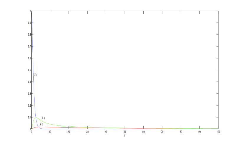
Figure 3.

Figure 4.

B. Some Two-summands Cases:

We consider next a principal orbit $G/K$ whose isotropy representation consists of two inequivalent ${\rm Ad}(K)$-invariant irreducible real summands. We assume that $K\subset H\subset G$ where $H,K$ are closed subgroups of the compact Lie group $G$ such that $H/K$ is a sphere. We choose a $G$-invariant background metric $\mathsf{b}$ on $G/K$ such that it induces the constant curvature $1$ metric on $H/K$. Our cohomogeneity one manifold $M$ is then the vector bundle $G\times_{H}\mbox{${\mathbb{R}}$}^{d_{1}+1}$ where $H/K\subset\mbox{${\mathbb{R}}$}^{d_{1}+1}$ is regarded as the unit sphere.

Let $\mbox{${\mathfrak{g}}$}=\mbox{${\mathfrak{k}}$}\oplus\mbox{${\mathfrak{p}}$}$ be an ${\rm Ad}(K)$-invariant decomposition of the Lie algebra of $G$. Then ${\mathfrak{p}}$ is identified with the tangent space of $G/K$ at the base point. We can further decompose ${\mathfrak{p}}$ as $\mbox{${\mathfrak{p}}$}_{1}\oplus\mbox{${\mathfrak{p}}$}_{2}$, where $\mbox{${\mathfrak{p}}$}_{i}$ are $\mathsf{b}$-orthogonal irreducible ${\rm Ad}(K)$-representations of dimensions $d_{i}$. Note that $\mbox{${\mathfrak{p}}$}_{1}$ is the tangent space to the sphere $H/K$ at the base point, and $\mbox{${\mathfrak{p}}$}_{2}$ is the tangent space of the singular orbit $G/H$ at the base point. Our metrics of cohomogeneity one then take the form

$$\bar{g}=dt^{2}+g_{1}(t)^{2}\;{\mathsf{b}}|\mbox{${\mathfrak{p}}$}_{1}+g_{2}(t)^{2}\;{\mathsf{b}}|\mbox{${\mathfrak{p}}$}_{2}.$$

As is well-known, the Ricci operator of the metric $g(t)$ on $G/K$ has corresponding components

$$r_{1}=\frac{A_{1}}{d_{1}}\frac{1}{g_{1}^{2}}+\frac{A_{3}}{d_{1}}\frac{g_{1}^{2}}{g_{2}^{4}}$$

$$r_{2}=\frac{A_{2}}{d_{2}}\frac{1}{g_{2}^{2}}-\frac{2A_{3}}{d_{2}}\frac{g_{1}^{2}}{g_{2}^{4}}.$$

As a result of our choice of $\mathsf{b}$, one has $A_{1}=d_{1}(d_{1}-1)$, and the constants $A_{2},A_{3}$ are analogous (but not always equal) to the quantities $c_{Q}$ and $\|{\mathcal{A}}\|$ in [DHW].

Taking $(z_{1},\ldots,z_{6}):=(g_{1},\dot{g_{1}},g_{2},\dot{g_{2}},u,\dot{u})$ as before, the soliton equations become

$$\dot{z_{1}} = z_{2}$$

$$\dot{z_{2}} = -(d_{1}-1)\frac{z_{2}^{2}}{z_{1}}-d_{2}\frac{z_{2}z_{4}}{z_{3}}+z_{2}z_{6}+\frac{d_{1}-1}{z_{1}}+\frac{A_{3}}{d_{1}}\frac{z_{1}^{3}}{z_{3}^{4}}+\frac{\epsilon}{2}z_{1}$$

$$\dot{z_{3}} = z_{4}$$

$$\dot{z_{4}} = -d_{1}\frac{z_{2}z_{4}}{z_{1}}-(d_{2}-1)\frac{z_{4}^{2}}{z_{3}}+z_{4}z_{6}+\frac{A_{2}}{d_{2}}\frac{1}{z_{3}}-2\frac{A_{3}}{d_{2}}\frac{z_{1}^{2}}{z_{3}^{3}}+\frac{\epsilon}{2}z_{3}$$

$$\dot{z_{5}} = z_{6}$$

$$\dot{z_{6}} = -z_{6}\left(d_{1}\frac{z_{2}}{z_{1}}+d_{2}\frac{z_{4}}{z_{3}}\right)+z_{6}^{2}+\epsilon z_{5}+C,$$

with $\epsilon=0$ and $C=-1$.

Example 2.   We set $G={\rm Sp}(m+1),H={\rm Sp}(m)\times{\rm Sp}(1),$ and $K={\rm Sp}(m)\times{\rm U}(1)$. The principal orbit $G/K$ is diffeomorphic to $\mbox{${\mathbb{C}}$}{\mbox{${\mathbb{P}}$}}^{2m+1}$ and the singular orbit $G/H$ is $\mbox{${\mathbb{H}}$}{\mbox{${\mathbb{P}}$}}^{m}$. So $d_{1}=2,d_{2}=4m$, and $A_{2}=2m(m+2),A_{3}=\frac{m}{2}$ (where $\mathsf{b}$ is given by $-2{\rm tr}(XY)$). As before we set $u(0)=0$ and (5.1) becomes $\ddot{u}(0)=-\frac{1}{3}$. The initial values of $(z_{1},\ldots,z_{6})$ are given by $(0,1,\bar{h},0,0,0)$ where $\bar{h}>0.$

We plot the functions $g_{i}$ and $u$ for the $m=1$ and $m=2$ cases respectively in Figures $5$ and $6$. Recall that the dimensions of the cohomogeneity one manifolds are respectively $7$ and $11$ for the $m=1$ and $m=2$ cases. The initial value $\bar{h}$ is taken to be $6$ in both cases. Again the soliton potential very quickly becomes approximately linear with slope close to $-1$. The growth of the functions $g_{i}$ is consistent with being like $\sqrt{t}$ asymptotically.

Figure 5.

Figure 6.

When the isotropy representation of the principal orbit is multiplicity free, we can still define the new variables $s$ and $X_{i},Y_{i}$ as in §2. We again let ${\tilde{X}_{i}}=X_{i}/\sqrt{d_{i}}$ and ${\tilde{Y}_{i}}=Y_{i}/\sqrt{d_{i}}$. Now we can plot the quantities ${\tilde{X}}_{i},{\tilde{Y}}_{i}$ against $t$. Figure $7$ corresponds to the $m=1$ case and Figure $8$ to the $m=2$ case. All these quantities appear to tend to zero, but the ${\tilde{X}}_{i}$ do so faster. Note that since by Proposition 1.14 the quantity $\xi$ tends to $1$, the fact that the ${\tilde{X}}_{i}$ appear to tend to zero very likely indicates that the shape operator $L$ also tends to $0$.

Figure 7. ${\tilde{X}_{i}},{\tilde{Y}_{i}}$ for $m=1$

Figure 8. ${\tilde{X}_{i}},{\tilde{Y}_{i}}$ for $m=2$

We can also plot the ratios ${\tilde{X}}_{1}/{\tilde{X}_{2}}=\frac{\dot{g_{1}}}{g_{1}}\frac{g_{2}}{\dot{g_{2}}}$ and ${\tilde{Y}}_{1}/{\tilde{Y}}_{2}=\frac{g_{2}}{g_{1}}$ against $t$. For the $m=1$ case this is shown in Figure 9. The first ratio appears to tend to $1$, which likely indicates that the principal curvatures of the principal orbits asymptotically become equal. It is not as convincing (from considering other values of $m$) that the second ratio tends to $1$, although it does appear to tend to some limit.

Figure 9. ${\tilde{X}_{1}}/{\tilde{X}_{2}}$ and ${\tilde{Y}_{1}}/{\tilde{Y}_{2}}$ for $m=1$

Similar numerical results hold for larger values of $m$.

Example 3.   We set $G={\rm Sp}(m+1)\times{\rm Sp}(1),H={\rm Sp}(m)\times{\rm Sp}(1)\times{\rm Sp}(1),$ and $K={\rm Sp}(m)\times\Delta{\rm Sp}(1)$. The principal orbit $G/K$ is diffeomorphic to $S^{4m+3}$ and the singular orbit $G/H$ is again $\mbox{${\mathbb{H}}$}{\mbox{${\mathbb{P}}$}}^{m}$. So $d_{1}=3,d_{2}=4m$, and $A_{2}=4m(m+2),A_{3}=\frac{3m}{4}$ (where $\mathsf{b}$ is given by $-{\rm tr}(XY)$ on both the ${\rm Sp}(m+1)$ and ${\rm Sp}(1)$ factors). As before we set $u(0)=0$ and (5.1) becomes $\ddot{u}(0)=-\frac{1}{4}$. The initial values of $(z_{1},\ldots,z_{6})$ are given by $(0,1,\bar{h},0,0,0)$ where $\bar{h}>0.$

For this case we obtain graphs very similar to those in Example 2.

Based on the last two examples, we would conjecture that on the vector bundles $G\times_{H}\mbox{${\mathbb{R}}$}^{d_{1}+1},$ where $(G,H,K)$ are as above, there is a $1$-parameter family of non-homothetic complete steady gradient Ricci solitons. We hope to pursue this and related questions in subsequent work.

References

- [ACGT] V. Apostolov, D. Calderbank, P. Gauduchon and C. Tønnesen-Friedman, Hamiltonian -forms in Kähler geometry IV: weakly Bochner-flat Kähler manifolds, Comm. Anal. Geom. 16, (2008), 91-126.
- [BB] L. Bérard Bergery, Sur des nouvelles variétés Riemanniennes d’Einstein, Publications de l’Institut Elie Cartan, Nancy, (1982).
- [Be] A. Besse, Einstein Manifolds, Ergebnisse der Mathematik und ihrer Grenzgebiete, 3. Folge, Band 10, Springer-Verlag, (1987).
- [Bo1] C. Böhm, Non-compact cohomogeneity one Einstein manifolds, Bull. Soc. Math. France, 122, (1999), 135-177.
- [Bo2] C. Böhm, Inhomogeneous Einstein metrics on low-dimensional spheres and other low-dimensional spaces, Invent. Math., 134, (1998), no. 1, 145-176.
- [BGK1] C. Boyer, K. Galicki and J. Kollár, Einstein metrics on spheres, Ann. Math., 162, (2005), 557-580.
- [BGK2] C. Boyer, K. Galicki and J. Kollár, Einstein metrics on exotic spheres in dimension and , Experiment. Math., 14, (2005), 59-64.
- [Br1] S. Brendle, Rotation symmetry of self-similar solutions to the Ricci flow, to appear in Invent. Math., arXiv:math.DG/1202.1264.
- [Br2] S. Brendle, Rotation symmetry of solitons in higher dimensions, to appear in J. Diff. Geom., arXiv:math.DG/1203.0270.
- [Bry] R. Bryant, unpublished work.
- [BryS] R. Bryant and S.M. Salamon, On the construction of some complete metrics with exceptional holonomy, Duke Math J., 58, (1989), 829-850.
- [Buz] M. Buzano, Initial value problem for cohomogeneity one gradient Ricci solitons, J. Geom. Phys, 61, (2011), 1033-44.
- [Cao] H. D. Cao, Existence of gradient Ricci solitons, Elliptic and Parabolic Methods in Geometry, A. K. Peters, (1996), 1-16.
- [Chen] B. L. Chen, Strong uniqueness of the Ricci flow, J. Diff. Geom., 82 , (2009),363-382.
- [Cetc] B. Chow, S.C. Chu, D. Glickenstein, C. Guenther, J. Isenberg, T. Ivey, D. Knopf, P. Lu, F. Luo, and L. Nei, The Ricci flow: techniques and applications Part I: geometric aspects, Mathematical Surveys and Monographs Vol. 135, American Math. Soc. (2007).
- [CGLP1] M. Cvetic̆, G. Gibbons, H. Lü and C. Pope, Supersymmetric -branes and manifolds, Nucl. Phys. B, 620, (2002), 3-28.
- [CGLP2] M. Cvetič, G. Gibbons, H. Lü and C. Pope, New complete noncompact manifolds, Nucl. Phys. B 620, (2002), 29-54.
- [DHW] A. Dancer, S. Hall and M. Wang, Cohomogeneity one shrinking Ricci solitons: an analytic and numerical study, Asian J. Math., 17, (2013), no. 1, 33-61.
- [DW1] A. Dancer and M. Wang, On Ricci solitons of cohomogeneity one, Ann. Glob. Anal. Geom., 39, (2011) 259-292.
- [DW2] A. Dancer and M. Wang, Some new examples of non-Kähler Ricci solitons, Math. Res. Lett. 16, (2009) 349-363.
- [DW3] A. Dancer and M. Wang, Non-Kähler expanding Ricci solitons, IMRN, (2009), 1107-33.
- [DW4] A. Dancer and M. Wang, The cohomogeneity one Einstein equations from the Hamiltonian viewpoint, J. reine angew. Math., 524, (2000), 97-128.
- [DW5] A. Dancer and M. Wang, Superpotentials and the cohomogeneity one Einstein equations, Comm. Math. Phys., 260, (2005), 75-115.
- [DW6] A. Dancer and M. Wang, Classification of superpotentials, Comm. Math. Phys., 284, (2008), 583-647.
- [DW7] A. Dancer and M. Wang, Classifying superpotentials: three summands case, J. Geom. Phys., 61, (2011), 675-692.
- [FIK] M. Feldman, T. Ilmanen, and D. Knopf, Rotationally symmetric shrinking and expanding gradient Kähler-Ricci solitons, J. Diff. Geom., 65, (2003), 169-209.
- [FR] M. Fernández-López and E. García-Río, Maximum principles and gradient Ricci solitons, J. Diff. Equations, 251, (2011), 73-81.
- [GPP] G. Gibbons, D. Page and C.N. Pope, Einstein metrics on , and bundles, Comm. Math. Phys., 127, (1990), 529-553.
- [Ha1] R. S. Hamilton, The Ricci flow on surfaces, in Mathematics and General Relativity (Santa Cruz, CA, 1986), Contemp Math., 71, Amer. Math. Soc., (1988), 237-262.
- [Ha2] R. S. Hamilton, Eternal solutions to the Ricci flow, Jour. Diff. Geom., 38, (1993), 1-11.
- [HHR] M. Hill, M. Hopkins and D. Ravenel, On the non-existence of elements of Hopf invariant one, arXiv:0908.3724v2.
- [Iv] T. Ivey, New examples of complete Ricci solitons, Proc. AMS, 122, (1994), 241-245.
- [Ko] N. Koiso, On Rotationally symmetric Hamilton’s equation for Kähler-Einstein metrics, Adv. Studies Pure Math., 18-I, Academic Press, (1990), 327-337.
- [KS] S. Kwaski and R. Schultz, Multiplication stablization and transformation groups, in Current Trends in Transformation Groups, K-Monogr. Math., Kluwer, (2002), 147-165.
- [MS] O. Munteanu and N. Sesum, On gradient Ricci solitons, J. Geom. Anal. 23, (2013), no. 2, 539-561.
- [Per] G. Perelman, The entropy formula for the Ricci flow and its geometric applications, arXiv:math.DG/0211159.
- [PRS] S. Pigola, M. Rimoldi and A. Setti, Remarks on non-compact gradient Ricci solitons, Math. Z., 268, (2011), 777-790.
- [PS] F. Podesta and A. Spiro, Kähler-Ricci solitons on homogeneous toric bundles, J. reine angew. Math, 642, (2010), 109-127.
- [S] R. Schultz, Smooth structures on , Ann. Math., 90, (1969), 187-198.
- [WZh] Xu-Jia Wang and Xiaohua Zhu, Kähler-Ricci solitons on toric manifolds with positive first Chern class, Adv. Math., 188, (2004), 87-103.
- [WeiWu] G. Wei and P. Wu, On volume growth of gradient steady Ricci solitons, arXiv:math.DG/1208.2040.
- [Wu] P. Wu, On potential function of gradient steady Ricci solitons, J. Geom. Anal., arXiv:math.DG/1102.3018.