Search for long-lived gravitational-wave transients coincident with long gamma-ray bursts

Abstract

Long gamma-ray bursts (GRBs) have been linked to extreme core-collapse supernovae from massive stars. Gravitational waves (GW) offer a probe of the physics behind long GRBs. We investigate models of long-lived ($\sim 10$–$1000\,\mathrm{s}$) GW emission associated with the accretion disk of a collapsed star or with its protoneutron star remnant. Using data from LIGO’s fifth science run, and GRB triggers from the Swift experiment, we perform a search for unmodeled long-lived GW transients. Finding no evidence of GW emission, we place $90\%$ confidence level upper limits on the GW fluence at Earth from long GRBs for three waveforms inspired by a model of GWs from accretion disk instabilities. These limits range from $F<3.5\,\mathrm{ergs\,cm^{-2}}$ to $F<1200\,\mathrm{ergs\,cm^{-2}}$, depending on the GRB and on the model, allowing us to probe optimistic scenarios of GW production out to distances as far as $\approx 33\,\mathrm{Mpc}$. Advanced detectors are expected to achieve strain sensitivities $10\times$ better than initial LIGO, potentially allowing us to probe the engines of the nearest long GRBs.

I Introduction

Gamma-ray bursts (GRBs) are divided into two classes (Kouveliotou et al., 1993; Gehrels et al., 2006). Short GRBs, lasting $\lesssim 2\,\mathrm{s}$ and characterized by hard spectra, are thought to originate primarily from the merger of binary neutron stars or from the merger of a neutron star with a black hole Eichler et al. (1989); Mochkovitch et al. (1993). On the other hand, long GRBs, lasting $\gtrsim 2\,\mathrm{s}$ and characterized by soft spectra, are associated with the extreme core collapse of massive stars (Campana et al., 2006; Pian et al., 2006; Soderberg et al., 2006; Mazzali et al., 2006). In the standard scenario, long GRBs are the product of a relativistic outflow, driven either by a black hole with an accretion disk or a protomagnetar (see, e.g., Thompson (1994); MacFadyen et al. (2001); Woosley (1993); Paczyński (1998)). At least two types of models have been proposed in which long GRBs may be associated with long-lived $\sim 10$–$1000\,\mathrm{s}$ gravitational-wave (GW) transients. One family of models relies on the formation of clumps in the accretion disk surrounding a newly formed black hole following core collapse Piro and Pfahl (2007); van Putten (2001, 2008); Bonnell and Pringle (1995); Kiuchi et al. (2011). The motion of the clumps generates long-lived narrowband GWs.

The second family of models relies on GW emission from a nascent protoneutron star. If the star is born spinning sufficiently rapidly Corsi and Mészáros (2009), or if it is spun up through fallback accretion Piro and Ott (2011); Piro and Thrane (2012), it may undergo secular or dynamical instabilities Chandrasekhar (1969); Owen and Lindblom (2002), which, in turn, are expected to produce long-lived narrowband GW transients Piro and Thrane (2012). Such rapidly spinning protoneutron stars have been invoked to help explain GRB afterglows Corsi and Mészáros (2009).

The goal of this work is to implement a search for generic long-lived GW transients coincident with long GRBs. While we are motivated by the two families of models discussed above, we make only minimal assumptions about our signal: that it is long-lived and that it is narrowband, producing a narrow track on a frequency-time ($ft$)-map.

Our analysis builds on previous searches for GWs from GRBs by the LIGO Abbott et al. (2009a) and Virgo Acernese, F. for the Virgo Collaboration (2006) detectors; (see more below). However, this analysis differs significantly from previous LIGO-Virgo GRB analyses Abbott et al. (2010); Abadie et al. (2010a, 2012a); Abbott et al. (2008a); Abadie et al. (2012b) since previous searches have focused on either short sub-second burst signals or modeled compact binary coalescence signals associated with short GRBs. Here, however, we consider unmodeled signals lasting $\sim 10$–$1000\,\mathrm{s}$ associated with the core-collapse death of massive stars.

During LIGO’s fifth science run (S5) (Nov. 5, 2005–Sep. 30, 2007) Abbott et al. (2009a), which provides the data for this analysis, GRBs were recorded by the Swift experiment Gehrels et al. (2004) at a rate of $\approx 100\,\mathrm{yr^{-1}}$ Gehrels et al. (2009). GRBs are most commonly detected at distances corresponding to redshifts $z\approx 1$–$2$ Gehrels et al. (2009), though, nearby GRBs have been detected as close as $37\,\mathrm{Mpc}$ (Galama et al., 1998). During S5, there were five nearby GRBs ($150$–$610\,\mathrm{Mpc}$) . Unfortunately, LIGO was not observing at the time of these GRBs despite a coincident detector duty cycle of $\approx 50\%$. While none of the GRBs analyzed here are known to be nearby (having a luminosity distance $D_{\text{luminosity}}<1000\,\mathrm{Mpc}$ and redshift $\lesssim 0.20$), the number of nearby GRBs during S5 bodes well for observing a nearby long GRB coincident with LIGO/Virgo data in the advanced detector era.

The remainder of this paper is organized as follows. In Section II we describe the LIGO observatories, in Section III we describe the methodology of our search, in Section IV we describe the salient features of our signal model. In Section V we describe our results and in Section VI we discuss implications and future work.

II The LIGO Observatories

We analyze data from the $4\,\mathrm{km}$ H1 and L1 detectors in Hanford, WA and Livingston, LA respectively. We use data from the S5 science run, during which LIGO achieved a strain sensitivity of $\approx 3\times 10^{-23}\,\mathrm{Hz^{-1/2}}$ in the most sensitive band between $\sim 100$–$200\,\mathrm{Hz}$ Abbott et al. (2009a). The H1L1 detector pair provides the most sensitive data available during S5, though a multibaseline approach remains a future goal .

S5 saw a number of important milestones (see, e.g., Abbott et al. (2008b, 2009b); H. Grote and the LIGO Scientific Collaboration (2010)), but most relevant for our present discussion are results constraining the emission of GWs from GRBs Abbott et al. (2010); Abadie et al. (2010a, 2012a); Abbott et al. (2008a) (see also Abadie et al. (2012b)). Previous results have limited the distance to long and short GRBs as a function of the available energy for generic waveforms Abbott et al. (2010); Abadie et al. (2012b) and also for compact binary coalescence waveforms Abadie et al. (2010a). They have investigated the origin of two GRBs that might have occurred in nearby galaxies Abadie et al. (2012a); Abbott et al. (2008a).

Currently LIGO Harry, G. M. for the LIGO Scientific Collaboration (2010); Iyer et al. (2011) and Virgo Acernese, F. for the Virgo Collaboration (2006) observatories are undergoing major upgrades that are expected to lead to a factor of ten improvement in strain sensitivity, and thus distance reach. The GEO detector H. Grote and the LIGO Scientific Collaboration (2010), meanwhile, continues to take data while the KAGRA detector Kuroda et al. (2010) is under construction. This paper sets the stage for the analysis of long-lasting transients from GRBs in the advanced detector era and demonstrates a long-transient pipeline Thrane et al. (2011); Prestegard et al. (2012) that is expected to have more general applications Piro and Thrane (2012).

III Method

We analyze GRB triggers—obtained through the Gamma-ray burst Coordinates Network GCN (2007) and consisting of trigger time, right ascension (RA), and declination (dec)—from the Swift satellite’s Burst Alert Telescope, which has an angular resolution of $\approx 0.02^{\circ}$–$0.07^{\circ}$ NASA Goddard Space Flight Center (2012) that is much smaller than the angular resolution of the GW detector network. This resolution allows us to study GW frequencies up to $1200\,\mathrm{Hz}$ while neglecting complications from GRB sky localization errors; see Prestegard et al. (2012).

LIGO data are pre-processed to exclude corrupt and/or unusable data Blackburn et al. (2008). In the frequency domain, we remove bins associated with highly non-stationary noise caused by known instrumental artifacts including $60\,\mathrm{Hz}$ harmonics and violin resonances Abbott et al. (2009a).

We define a $\left[-600\,\mathrm{s},+900\,\mathrm{s}\right]$ on-source region around each GRB trigger. The GW signal is assumed to exist only in the on-source region. The $-600\,\mathrm{s}$ allows for possible delays between the formation of a compact remnant object and the emission of the gamma rays (see Abadie et al. (2012b) and references therein). The $+900\,\mathrm{s}$ is motivated by the hypothesis that GW production is related to GRB afterglows Corsi and Mészáros (2009), which can extend $\approx 10$–$10^{4}\,\mathrm{s}$ after the initial GRB trigger, though most often the duration is $\lesssim 1000\,\mathrm{s}$ Panaitescu and Vestrand (2008) .

Of the $131$ long ($t_{90}>2\,\mathrm{s}$) GRB triggers  detected by the Swift satellite Gehrels et al. (2004) during S5, there are $29$ for which coincident H1L1 data are available for the entire $1500\,\mathrm{s}$ on-source region. We analyze an additional $21$ GRB triggers for which $\geq 1000\,\mathrm{s}$ of coincident H1L1 data are available (but not all $1500\,\mathrm{s}$) and hence searchable for signal, though, we do not include them in our upper-limit calculations described below.

We additionally require that the GRB is not located in a direction with poor network sensitivity, which can prevent the detection of even a loud signal (see the appendix for details). Only one GRB is excluded on account of this requirement.

We consider a frequency range of $100$–$1200\,\mathrm{Hz}$, above which we cannot, at present, probe astrophysically interesting distances due to the increase in detector noise at high frequencies and the fact that strain amplitude falls like $1/f$ for a fixed energy budget. Frequencies $\lesssim 100\,\mathrm{Hz}$ are excluded since non-stationary noise in this band diminishes the sensitivity of the search; see Prestegard et al. (2012).

Following Thrane et al. (2011), strain data from the $1100\,\mathrm{Hz}\times 1500\,\mathrm{s}$ on-source region is converted to spectrograms ($ft$-maps) of strain cross- and auto-power spectra. These $ft$-maps utilize Hann-windowed, $1\,\mathrm{s}$, $50\%$-overlapping segments with a frequency resolution of $1\,\mathrm{Hz}$ (see also van Putten (2001)). The strain cross-power is given by Thrane et al. (2011):

$$\hat{Y}(t;f) \equiv \frac{2}{\cal N}\text{Re}\left[Q_{IJ}(t;f,\hat{\Omega})\,\tilde{s}_{I}^{\star}(t;f)\tilde{s}_{J}(t;f)\right].$$ (1)

Here $t$ is the segment start time, $f$ is the frequency bin, ${\cal N}$ is a window normalization factor, $\hat{\Omega}$ is the search direction, and $\tilde{s}_{I}(t;f)$, $\tilde{s}_{J}(t;f)$ are discrete Fourier transforms of strain data for segment $t$ using detectors $I=\text{H1}$ and $J=\text{L1}$ respectively. $Q_{IJ}(t;f,\hat{\Omega})$ is a filter function, which takes into account the time delay between the detectors and their directional response; (see Thrane et al. (2011) for additional details). The dependence of $\hat{Y}(t;f)$ on $\hat{\Omega}$ is implicit for the sake of notational compactness. An estimator for the variance of $\hat{Y}(t;f)$ is given by Thrane et al. (2011):

$$\hat{\sigma}^{2}(t;f) \equiv \frac{1}{2}\left|Q_{IJ}(t;f,\hat{\Omega})\right|^{2}P_{I}^{\prime}(t;f)P_{J}^{\prime}(t;f),$$ (2)

where $P_{I}^{\prime}(t;f)$ and $P_{J}^{\prime}(t;f)$ are the auto-powers measured in detectors $I$ and $J$, respectively and the prime denotes that they are calculated using the average of $n=8$ segments neighboring the one beginning at $t$ (four on each side).

Using Eqs. 1 and 2, we cast our search for long GW transients as a pattern recognition problem (see Fig. 1). GW signals create clusters of positive-valued pixels in $ft$-maps of signal-to-noise ratio:

$$\text{SNR}(t;f)\equiv\hat{Y}(t;f)/\hat{\sigma}(t;f),$$ (3)

whereas noise is randomly distributed with a mean of $\langle\text{SNR}(t;f)\rangle=0$.

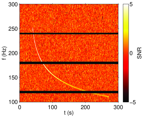
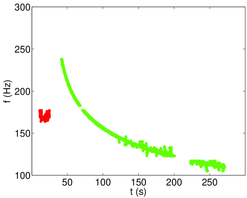
Figure 1: Recovery of a simulated waveform in time-shifted noise. Left: $ft$-map of $\text{SNR}(t;f)$ for an injected accretion disk instability signal (model $c$). The horizontal black lines are removed frequency bins corresponding to instrumental artifacts. Right: significant clusters recovered with the clustering algorithm. Here the green cluster is due to injected GW signal while the red cluster is due to a noise fluctuation. In this example, the recovered $\text{SNR}_{\text{tot}}=290$ for the largest cluster (due to the GW signal) is well above the threshold of $30$ while noise fluctuations, such as the small red blob shown here, have typical recovered $\text{SNR}_{\text{tot}}=17$. (Note that the left-hand side color scale shows $\text{SNR}(t;f)$, defined in Eq. 3 for each pixel, whereas $\text{SNR}_{\text{tot}}$, defined in Eq. 4, is a property of a cluster consisting of many pixels.)

We employ a track-search clustering algorithm for generic narrowband waveforms Prestegard and Thrane (2012), which works by connecting $ft$-map pixels above a threshold and that fall within a fixed distance of nearby above-threshold pixels. Clusters (denoted $\Gamma$) are ranked by the value of the total cluster signal-to-noise ratio $\text{SNR}_{\text{tot}}$:

$$\text{SNR}_{\text{tot}}=\frac{\sum_{t;f\in\Gamma}\hat{Y}(t;f)\,\hat{\sigma}^{-2}(t;f)}{\left(\sum_{t;f\in\Gamma}\hat{\sigma}^{-2}(t;f)\right)^{1/2}}.$$ (4)

To evaluate the significance of the cluster with the highest $\text{SNR}_{\text{tot}}$ in the on-source region, we compare it to the background distribution, which is estimated using time-shifted data.

Time shifts, in which we offset the H1 and L1 strain series by an amount greater than the intersite GW travel time, provide a robust method of estimating background Abbott et al. (2004). For each value of $\text{SNR}_{\text{tot}}$ we assign a false-alarm probability $p$ by performing many trials with time-shifted data (see Fig. 2). The false-alarm probability for $\text{SNR}^{\prime}_{\text{tot}}$ is given by the fraction of time-shifted trials for which we observed $\text{SNR}_{\text{tot}}\geq\text{SNR}^{\prime}_{\text{tot}}$. We apply a noise transient identification algorithm Prestegard et al. (2012) in order to mitigate contamination from non-stationary noise. Similar consistency-check noise transient identification is performed in previous searches for unmodeled GW, e.g., Abbott et al. (2010). The relatively good agreement in Fig. 2 between time-shifted and Monte Carlo data (colored Gaussian strain noise) is attributable in part to the stability of LIGO strain noise for frequencies $>100\,\mathrm{Hz}$ on long time scales Prestegard et al. (2012).

Using time-shifted data, we determine the interesting-candidate threshold $\text{SNR}_{\text{tot}}^{\text{th}}$ such that the probability of observing any of the 50 GRB triggers with $\text{SNR}_{\text{tot}}>\text{SNR}_{\text{tot}}^{\text{th}}$ due to noise fluctuations is $<1\%$. We find that the threshold for an interesting candidate is $\text{SNR}_{\text{tot}}^{\text{th}}=30$. Interesting candidates, if they are observed, are subjected to further study.

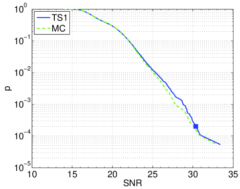
Figure 2: Single-trigger false-alarm probability $p$ vs. $\text{SNR}_{\text{tot}}$ for time-shifted (TS) and Monte Carlo (MC) data. The marker indicates $\text{SNR}_{\text{tot}}^{\text{th}}$, the threshold for an interesting candidate for follow-up. $\text{SNR}_{\text{tot}}^{\text{th}}$ is defined such that the probability of observing any of the 50 GRB triggers with $\text{SNR}_{\text{tot}}>\text{SNR}_{\text{tot}}^{\text{th}}$ due to noise fluctuations is $<1\%$.

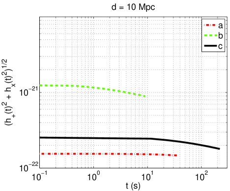
Figure 3: Strain amplitude $[h_{+}^{2}(t)+h_{\times}^{2}(t)]^{1/2}$ vs. time for the waveforms in Table 1 assuming a reference distance of $10\,\mathrm{Mpc}$.

IV Signal models

In order to constrain physical parameters such as fluence in the absence of a GW detection, it is necessary to have a waveform model. In cases where there is no trusted waveform, one must employ a toy model which is believed to encompass the salient features of the astrophysical phenomenology, such as the sine-Gaussians used in short GW burst analyses Abadie et al. (2012b).

For our toy model, we employ accretion disk instability (ADI) waveforms Santamaría and Ott (2011) (based on van Putten (2001, 2008) and references therein) in which a spinning black hole of mass $M$ (with typical values $3M_{\odot}-10M_{\odot}$) drives turbulence in an accretion torus of mass $m\approx 1.5M_{\odot}$. This turbulence causes the formation of clumps of mass $\epsilon m$ (with typical values $0.015M_{\odot}-0.3M_{\odot}$), the motion of which emits GWs. In optimistic models, as much as $E_{\text{GW}}=0.1M_{\odot}c^{2}$ is emitted in GWs van Putten (2001). We emphasize that, like the sine-Gaussian waveforms used in short GW burst analyses, these waveforms should be taken as toy model representations of a GW signal for which there is significant theoretical uncertainty.

The model is additionally parameterized by a dimensionless spin parameter $a^{\star}\equiv(c/G)J_{\text{BH}}/M^{2}$, bounded by $[0,1)$, where $J_{\text{BH}}$ is the angular momentum of the black hole Santamaría and Ott (2011). An $ft$-map of $\text{SNR}(t;f)$ illustrating an injected ADI waveform with parameters $M=10M_{\odot}$, $m=1.5M_{\odot}$, $\epsilon=0.04$ and $a^{\star}=0.95$ (model $c$) is shown in the left-hand panel of Fig. 1. (The GW frequency decreases with time as the black hole spins down and the innermost stable circular orbit changes.) The waveforms are calculated assuming a circularly polarized source (inclination angle $\iota\approx 0$), which is a reasonable assumption given that long GRBs are thought to be observed almost parallel to the angular momentum vector Gal-Yam et al. (2006); Racusin et al. (2009).

We utilize different combinations of parameters to create three waveforms (denoted $a$, $b$, and $c$), which are summarized in Table 1 and Fig. 3. By varying the model parameters, we obtain signals of varying durations ($9$–$231\,\mathrm{s}$). For these three waveforms we constrain GW fluence—the GW energy flowing through a unit area at the detector integrated over the emission time. The fluence is defined as:

$$F\equiv\frac{c^{3}}{16\pi G}\int dt\left(\dot{h}_{+}^{2}(t)+\dot{h}_{\times}^{2}(t)\right).$$ (5)

By assuming a fixed GW energy budget $E_{\text{GW}}=0.1M_{\odot}c^{2}$, it is possible to cast the fluence limits as limits on the distance $D$ to the GRB. The relationship between fluence, distance, and energy is given by

$$D=\left(\frac{5}{2}\frac{E_{\text{GW}}}{4\pi F}\right)^{1/2}.$$ (6)

The factor of $5/2$ arises from the assumption that the source emits face-on, which causes modest enhancement in observed fluence compared to a source observed edge-on.

ID	$M$	$a^{\star}$	$\epsilon$	$m$	$t_{\text{dur}}$	$f$ (Hz)
a	5	$0.3$	$0.05$	$1.5$	$39$	131–171
b	10	$0.95$	$0.2$	$1.5$	$9$	90–284
c	10	$0.95$	$0.04$	$1.5$	$231$	105–259

Table 1: Parameters for waveforms Santamaría and Ott (2011) inspired by van Putten (2001, 2008). $M$ is black hole mass in units of $M_{\odot}$, $a^{\star}$ is a dimensionless spin parameter, $\epsilon$ is the fraction of torus mass that clumps, and $m$ is the torus mass in units of $M_{\odot}$. The free parameters ($M$, $a^{\star}$, $\epsilon$, $m$) are selected within the range of expected values in order to produce a range of signal durations.

V results

Properties of the loudest cluster for each GRB trigger including its signal-to-noise ratio $\text{SNR}_{\text{tot}}$ and its false-alarm probability $p$ are given in Table 2. Of the $50$ GRB triggers analyzed in this study, the most significant was GRB 070621 with $\text{SNR}_{\text{tot}}=24$ corresponding to a single-trigger false-alarm probability of $p=2.3\%$. The probability of observing $\text{SNR}_{\text{tot}}\geq 24$ among our $50$ GRB triggers is $69\%$.

Since we find no evidence of long-lived GW transients, we set $90\%$ confidence level (CL) upper limits on the GW fluence for each GRB trigger for the three test models considered. To calculate these limits we perform pseudo experiments in which we inject waveforms $a$, $b$, and $c$. All three waveforms are normalized to a fixed energy budget $E_{\text{GW}}=0.1M_{\odot}$ by multiplying each strain time series by a constant . We vary the distance to the source in order to determine the distance for which $90\%$ of the injected signals are recovered with an $\text{SNR}_{\text{tot}}$ exceeding the loudest cluster in the on-source region. From these distance limits, we obtain fluence limits from Eq. 6.

GW strain measurements are subject to systematic calibration uncertainties. For S5 H1,L1 and for $f<2000\,\mathrm{Hz}$, this error is estimated to be $10.4\%,14.4\%$ in amplitude Abadie et al. (2010b). In order to take calibration error into account in our upper limit calculation, we assume the true fluence is some number $\lambda$ times the measured fluence, and that $\lambda$ is Gaussian distributed with a mean of $1$ and a width of $\sqrt{10.4\%^{2}+14.4\%^{2}}=17.8\%$. Marginalizing over $\lambda$ leads to a $15\%$ reduction in our distance sensitivity. Phase and timing calibration errors are negligible for this analysis Abadie et al. (2010b).

The $90\%$ CL limits for models $a,b,$ and $c$ are reported in Table 3. We report upper limits on fluence and lower limits on distance assuming a GW energy budget of $E_{\text{GW}}=0.1M_{\odot}c^{2}$. For model $a$, we place upper limits on GW fluence of $3.5$–$1000\,\mathrm{ergs\,cm^{-2}}$ (corresponding to distance lower limits of $1.9$–$33\,\mathrm{Mpc}$). For model $b$, the corresponding limits are $F<4.4$–$410\,\mathrm{ergs\,cm^{-2}}$ ($D>3.0$–$29\,\mathrm{Mpc}$), and for model $c$, $F<16$–$1200\,\mathrm{ergs\,cm^{-2}}$ ($D>1.8$–$15\,\mathrm{Mpc}$). The variation in limits for a given model is due primarily to the direction-dependent antenna response factors, which cause $\sigma(t;f)$ to vary by two orders of magnitude for different search directions. The GRB for which we set the best limits is GRB 070611 while the least sensitive limits are placed on GRB 070107.

Given a fixed waveform with an overall normalization constant, fluence limits are proportional to limits on (the square) of the root-sum-squared strain

$$h_{\text{rss}}^{2}\equiv\int dt\left(h_{+}^{2}(t)+h_{\times}^{2}(t)\right)=kF,$$ (7)

where $k$ is a waveform-dependent constant. Using this relation, we can alternatively present the limits as

$$\begin{split}h^{a}_{\text{rss}}<7.0\times 10^{-22}(F/3.5\,\mathrm{erg\,cm^{-2}})^{1/2}\\ h^{b}_{\text{rss}}<7.7\times 10^{-22}(F/4.4\,\mathrm{erg\,cm^{-2}})^{1/2}\\ h^{c}_{\text{rss}}<1.5\times 10^{-21}(F/16\,\mathrm{erg\,cm^{-2}})^{1/2}\end{split}$$ (8)

The superscript of $h_{\text{rss}}$ refers to the different models.

VI Implications and future work

In the most optimistic scenarios for the production of GWs in stellar collapse, it has been claimed that as much as $E_{\text{GW}}=0.1M_{\odot}c^{2}$ of energy is converted into GWs van Putten (2001). The GW signature from the actual core collapse, as opposed to subsequent emission from an accretion disk or from a protoneutron star remnant, is expected to be significantly less energetic, with a typical energy budget of $E_{\text{GW}}=\sim 10^{-11}$–$10^{-7}M_{\odot}$ Ott (2009).

By comparing our best fluence upper limits $F^{90\%}=3.5\,\mathrm{ergs\,cm^{-2}}$ (GRB070611, model $a$) with this prediction, we extrapolate approximate distance lower limits as a function of frequency for this best-case scenario; see Fig. 4. In the most sensitive frequency range between $100$–$200\,\mathrm{Hz}$, the limits are as large as $D^{90\%}=33\,\mathrm{Mpc}$. They fall like $D^{90\%}\propto f^{-2}$ above $200\,\mathrm{Hz}$ due to increasing the detector shot noise as well as from the relationship between energy and strain $E_{\text{GW}}\propto f^{2}h^{2}$. The limits in Fig. 4 scale like $D^{90\%}\propto E_{\text{GW}}^{1/2}$ and $D^{90\%}\propto(F^{90\%})^{-1/2}$. The GW power spectral peak frequency is marked with a red circle. Note that the waveforms we consider here are not characterized by a single frequency, and so Fig. 4 should be taken as an approximate indicator of how results scale with frequency.

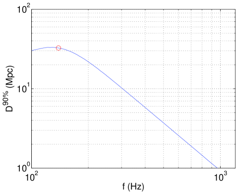
Figure 4: Best-case-scenario, approximate $90\%$ CL lower limits on the distance to sources of long-lived GW transients extrapolated from fluence upper limits. Following van Putten (2001), we assume a GW energy budget of $0.1M_{\odot}c^{2}$. The limits are calculated using the best fluence constraints from Table 3: $F^{90\%}=3.5\,\mathrm{ergs\,cm^{-2}}$ from GRB070611, model $a$. The GW power spectral peak is marked with a red circle. The frequency dependence should be taken as indicating an approximate trend as our waveforms are not monochromatic. Also, the extrapolation assumes a smooth detector noise curve, which only approximates the LIGO detector noise.

If the GW frequency is high ($f\gtrsim 1\,\mathrm{kHz}$) van Putten (2001), the reach of initial LIGO is only $\lesssim 1\,\mathrm{Mpc}$ due to the fact that distance sensitivity falls off rapidly with frequency: $D\propto f^{-2}$. The nearest GRB in our set with a known redshift measurement, GRB 070420, is estimated to have occurred at $z=0.48$–$0.93$ ($D_{\text{luminosity}}=2800$–$6400\,\mathrm{Mpc}$) Xiao and Schaefer (2011), well beyond our exclusion distances even for lower-frequency emission.

While we are therefore unable to rule out the most extreme models of GW emission with the present analysis, we have demonstrated that initial LIGO can test optimistic models out to distances as far as $\approx 33\,\mathrm{Mpc}$ depending on the GW frequency and the detector orientation during the time of the GRB. Advanced LIGO and Advanced Virgo are expected to achieve strain sensitivities $10\times$ better than the initial LIGO data analyzed here, which will be sufficient to test extreme models out to $D\approx 330\,\mathrm{Mpc}$. As discussed in Section I, GRBs are not infrequent at such distances .

Meanwhile, work is ongoing to develop more sophisticated data analysis procedures, to further enhance sensitivity. By tuning our analysis pipeline Thrane et al. (2011) for long-lived signals, we estimate that we can detect ADI waveforms for sources that are twice as distant as could have been detected by previous searches tuned for short signals Abbott et al. (2010); Abadie et al. (2012b) (corresponding to an increase in detection volume of $\approx 8\times$). In order to achieve additional improvements in sensitivity, work is ongoing to explore alternative pattern recognition strategies that relax the requirement that $\text{SNR}(t;f)$ exceeds some threshold to form a pixel cluster (see Eq. 3).

Long GRBs are by no means the only interesting source of long GW transients. In Piro and Ott (2011); Piro and Thrane (2012) it was argued that core-collapse supernovae can trigger the production of long-lived GW emission through fallback accretion. While the predicted strains are much less than the most extreme models considered here, the local rate of supernovae is much higher than the local rate of long GRBs, and preliminary sensitivity estimates suggest that fallback accretion-powered signals are interesting targets for Advanced LIGO/Virgo Piro and Thrane (2012). Other scenarios for long-lived GW production explored in Thrane et al. (2011), including protoneutron star convection and eccentric black hole binaries, remain areas of investigation. This analysis paves the way for future studies probing unmodeled long-lived GW emission.

	GRB	GPS	RA (hr)	DEC (deg)	${\bf t_{90}(s)}$	All data?	${\bf\text{SNR}_{\text{tot}}}$	$p$ (%)
1	GRB060116	821435861	5.65	-5.45	105.9	no	16	89.1
2	GRB060322	827103635	18.28	-36.82	221.5	no	18	49.7
3	GRB060424	829887393	0.49	36.79	37.5	yes	20	27.5
4	GRB060427	830173404	8.28	62.65	64.0	no	16	87.5
5	GRB060428B	830249692	15.69	62.03	57.9	yes	16	85.8
6	GRB060510B	831284548	15.95	78.60	275.2	no	18	55.5
7	GRB060515	831695286	8.49	73.56	52.0	no	18	59.1
8	GRB060516	831797028	4.74	-18.10	161.6	no	17	84.9
9	GRB060607B	833758378	2.80	14.75	31.1	yes	21	21.4
10	GRB060707	836343033	23.80	-17.91	66.2	no	18	46.9
11	GRB060714	836925134	15.19	-6.54	115.0	no	24	3.1
12	GRB060719	837327050	1.23	-48.38	66.9	yes	17	70.0
13	GRB060804	838711713	7.48	-27.23	17.8	no	18	55.2
14	GRB060807	838996909	16.83	31.60	54.0	no	22	10.1
15	GRB060813	839544636	7.46	-29.84	16.1	yes	18	50.7
16	GRB060814	839631753	14.76	20.59	145.3	no	21	16.7
17	GRB060908	841741056	2.12	0.33	19.3	yes	19	43.4
18	GRB060919	842687332	18.46	-50.99	9.1	no	19	43.2
19	GRB060923B	843046700	15.88	-30.91	8.6	no	21	18.3
20	GRB061007	844250902	3.09	-50.50	75.3	yes	18	47.2
21	GRB061021	845480361	9.68	-21.95	46.2	yes	20	30.9
22	GRB061102	846464445	9.89	-17.00	45.6	no	19	43.7
23	GRB061126	848566090	5.77	64.20	70.8	no	22	7.9
24	GRB061202	849082318	7.01	-74.59	91.2	yes	20	32.2
25	GRB061218	850449919	9.95	-35.22	6.5	no	17	75.8
26	GRB061222B	850795876	7.02	-25.86	40.0	yes	21	16.6
27	GRB070107	852206732	10.63	-53.20	347.3	yes	18	53.4
28	GRB070110	852448975	0.06	-52.98	88.4	yes	16	88.4
29	GRB070208	854961048	13.19	61.95	47.7	yes	22	13.0
30	GRB070219	855882630	17.35	69.34	16.6	yes	17	75.6
31	GRB070223	856228514	10.23	43.13	88.5	yes	18	58.2
32	GRB070318	858238150	3.23	-42.95	74.6	yes	20	24.9
33	GRB070330	859330305	17.97	-63.80	9.0	yes	16	95.7
34	GRB070412	860376437	12.10	40.13	33.8	yes	17	74.8
35	GRB070420	861085107	8.08	-45.56	76.5	yes	20	27.5
36	GRB070427	861697882	1.92	-27.60	11.1	yes	19	40.0
37	GRB070506	862464972	23.15	10.71	4.3	yes	21	20.6
38	GRB070508	862633111	20.86	-78.38	20.9	yes	18	48.9
39	GRB070509	862714121	15.86	-78.66	7.7	yes	17	84.6
40	GRB070520B	863718307	8.13	57.59	65.8	no	18	55.7
41	GRB070529	864478122	18.92	20.65	109.2	yes	17	78.6
42	GRB070611	865562247	0.13	-29.76	12.2	yes	22	7.9
43	GRB070612B	865664491	17.45	-8.75	13.5	no	17	77.5
44	GRB070621	866503073	21.59	-24.81	33.3	yes	24	2.3
45	GRB070714B	868424383	3.86	28.29	64.0	yes	19	38.8
46	GRB070721B	869049242	2.21	-2.20	340.0	yes	20	33.3
47	GRB070805	870378959	16.34	-59.96	31.0	yes	17	82.0
48	GRB070911	873525478	1.72	-33.48	162.0	no	18	59.4
49	GRB070917	874049650	19.59	2.42	7.3	no	19	37.7
50	GRB070920B	874357486	0.01	-34.84	20.2	no	22	8.4

Table 2: Swift long GRB triggers coincident with S5 H1L1 data and associated GW search results. “All data?” asks whether there is coincident LIGO data for all $1500\,\mathrm{s}$ in the on-source region (yes) or for just some of it (no). $\text{SNR}_{\text{tot}}$ is the signal-to-noise ratio for the loudest cluster and $p$ is the single-trial false alarm probability.

	90% UL on $F$ ($\mathrm{ergs\,cm^{-2}}$)			90% LL on $D$ ($\mathrm{Mpc}$)
ID	model			model
	a	b	c	a	b	c
GRB060424	20	25	71	14	12	7.2
GRB060428B	4.9	8.7	21	28	21	13
GRB060607B	94	120	330	6.3	5.7	3.3
GRB060719	20	30	71	14	11	7.3
GRB060813	25	26	74	12	12	7.1
GRB060908	5.6	6.9	20	26	23	14
GRB061007	120	180	620	5.6	4.6	2.5
GRB061021	21	26	89	13	12	6.5
GRB061202	15	22	64	16	13	7.7
GRB061222B	1000	80	280	1.9	6.8	3.7
GRB070107	270	410	1200	3.7	3.0	1.8
GRB070110	6.7	8.3	29	24	21	11
GRB070208	4.4	5.5	16	29	26	15
GRB070219	14	21	59	16	14	8.0
GRB070223	13	16	47	17	15	8.9
GRB070318	4.9	6.1	21	28	25	13
GRB070330	3.7	5.5	16	32	26	15
GRB070412	5.9	8.8	25	25	21	12
GRB070420	25	22	74	12	13	7.1
GRB070427	4.4	5.5	16	29	26	15
GRB070506	15	22	54	16	13	8.4
GRB070508	6.1	9.1	26	25	20	12
GRB070509	7.9	12	34	22	18	11
GRB070529	9.0	11	32	20	18	11
GRB070611	3.5	4.4	15	33	29	16
GRB070621	4.6	4.7	16	29	28	15
GRB070714B	46	69	160	9.0	7.4	4.8
GRB070721B	9.6	14	41	20	16	9.6
GRB070805	8.0	14	34	22	16	10

Table 3: Summary of fluence and distance constraints for waveforms a, b, and c. Distance limits are calculated assuming $E_{\text{GW}}=0.1M_{\odot}c^{2}$.

Appendix A Directional sensitivity cut

The pipeline used in this analysis works by comparing $\hat{Y}(t;f)$ (Eq. 1) to $\sigma(t;f)$ (Eq. 2), which depends on the auto-power in the four neighboring segments on each side of $t$; (for additional details see Thrane et al. (2011)). For a fixed direction on the sky $\hat{\Omega}$, the expectation value of $\text{SNR}(t;f)\equiv\hat{Y}(t;f)/\sigma(t;f)$ for one such pixel depends on the “pair efficiency” $\epsilon_{IJ}$ for each detector pair

$$\langle\text{SNR}(t;f)\rangle\propto\frac{\epsilon_{12}(t;\hat{\Omega})}{\left[\epsilon_{11}(t;\hat{\Omega})\epsilon_{22}(t;\hat{\Omega})\right]^{1/2}}.$$ (9)

Pair efficiency is defined in terms of the antenna response factors (see, e.g., Thrane et al. (2011))

$$\epsilon_{IJ}(t;\hat{\Omega})\equiv\frac{1}{2}\sum_{A}F^{A}_{I}(t,\hat{\Omega})F^{A}_{J}(t,\hat{\Omega}).$$ (10)

For a small subset of directions $\hat{\Omega}$, the following condition is met

$$\epsilon_{12}\ll\left(\epsilon_{11}(t;\hat{\Omega})\epsilon_{22}(t;\hat{\Omega})\right)^{1/2},$$ (11)

which means the GW signal produces a much stronger auto-power spectra compared to the cross-power spectra. In the most extreme cases, the GW signal in the segments neighboring $t$ causes $\sigma(t;f)\gg\hat{Y}(t;f)$, which makes $\text{SNR}(t;f)\approx 0$ even for loud signals.

To avoid searching in directions for which we are blind to GWs and can therefore not set limits, we employ a cut that ensures that GW signals can produce seed pixels with $\text{SNR}(t;f)\gtrsim 1$:

$$\epsilon_{12}\geq\frac{1}{4}\left(\epsilon_{11}(t;\hat{\Omega})\epsilon_{22}(t;\hat{\Omega})\right)^{1/2}.$$ (12)

We find that this cut eliminates GRB triggers for which we cannot set effective limits while removing only one out of $51$ GRB triggers.

References

- Kouveliotou et al. (1993) C. Kouveliotou, C. A. Meegan, G. J. Fishman, et al., Astrophys. J. Lett. 413, L101 (1993).
- Gehrels et al. (2006) N. Gehrels, J. P. Norris, S. D. Barthelmy, et al., Nature 444, 1044 (2006).
- Eichler et al. (1989) D. Eichler, M. Livio, T. Piran, and D. N. Schramm, Nature 340, 126 (1989).
- Mochkovitch et al. (1993) R. Mochkovitch, M. Hernanz, J. Isern, and X. Martin, Nature 361, 236 (1993).
- Campana et al. (2006) S. Campana et al., Nature 442, 1008 (2006).
- Pian et al. (2006) E. Pian et al., Nature 442, 1011 (2006).
- Soderberg et al. (2006) A. M. Soderberg et al., Nature 442, 1014 (2006).
- Mazzali et al. (2006) P. A. Mazzali et al., Nature 442, 1018 (2006).
- Thompson (1994) C. Thompson, MNRAS 270, 480 (1994).
- MacFadyen et al. (2001) A. I. MacFadyen, S. E. Woosley, and A. Heger, Astrophys. J. 550, 410 (2001).
- Woosley (1993) S. E. Woosley, Astrophys. J. 405, 273 (1993).
- Paczyński (1998) B. Paczyński, Astrophys. J. Lett. 494, L45 (1998).
- Piro and Pfahl (2007) A. L. Piro and E. Pfahl, Astrophys. J. 658, 1173 (2007).
- van Putten (2001) M. H. P. M. van Putten, Phys. Rev. Lett. 87, 091101 (2001).
- van Putten (2008) M. H. P. M. van Putten, Astrophys. J. Lett. 684, 91 (2008).
- Bonnell and Pringle (1995) I. A. Bonnell and J. E. Pringle, MNRASL 273, L12 (1995).
- Kiuchi et al. (2011) K. Kiuchi et al., Phys. Rev. Lett. 106, 251102 (2011).
- Corsi and Mészáros (2009) A. Corsi and P. Mészáros, Astrophys. J. 702, 1171 (2009).
- Piro and Ott (2011) A. L. Piro and C. D. Ott, Astrophys. J. 736, 1171 (2011).
- Piro and Thrane (2012) A. L. Piro and E. Thrane, Astrophys. J. 761, 63 (2012).
- Chandrasekhar (1969) S. Chandrasekhar, The Silliman Foundation Lectures (Yale University Press, 1969).
- Owen and Lindblom (2002) B. Owen and L. Lindblom, Classical Quantum Gravity 19, 1247 (2002).
- Abbott et al. (2009a) B. P. Abbott et al., Rep. Prog. Phys. 72, 076901 (2009a).
- Acernese, F. for the Virgo Collaboration (2006) Acernese, F. for the Virgo Collaboration, Classical Quantum Gravity 23, S63 (2006).
- Abbott et al. (2010) B. P. Abbott et al., Astrophys. J. 715, 1438 (2010).
- Abadie et al. (2010a) J. Abadie et al., Astrophys. J. 715, 1453 (2010a).
- Abadie et al. (2012a) J. Abadie et al., forthcoming in Astrophys. J. (2012a), eprint http://arxiv.org/abs/1201.4413.
- Abbott et al. (2008a) B. Abbott et al., Astrophys. J. 681, 1419 (2008a).
- Abadie et al. (2012b) J. Abadie et al., Astrophys. J. 760, 12 (2012b).
- Gehrels et al. (2004) N. Gehrels et al., Astrophys. J. 611, 1005 (2004).
- Gehrels et al. (2009) N. Gehrels, E. Ramirez-Ruiz, and D. B. Fox, Annu. Rev. Astron. Astrophys. 47, 567 (2009).
- Galama et al. (1998) T. J. Galama, P. M. Vreeswijk, J. van Paradijs, et al., Nature 385, 670 (1998).
- Abbott et al. (2008b) B. Abbott et al., Astrophys. J. Lett. 683, 45 (2008b).
- Abbott et al. (2009b) B. Abbott et al., Nature 460, 990 (2009b).
- H. Grote and the LIGO Scientific Collaboration (2010) H. Grote and the LIGO Scientific Collaboration, Classical Quantum Gravity 27, 084003 (2010).
- Harry, G. M. for the LIGO Scientific Collaboration (2010) Harry, G. M. for the LIGO Scientific Collaboration, Classical Quantum Gravity 27, 084006 (2010).
- Iyer et al. (2011) B. Iyer et al. (2011), lIGO-India Tech. rep. https://dcc.ligo.org/cgi-bin/DocDB/ShowDocument?docid=75988.
- Kuroda et al. (2010) K. Kuroda et al., Classical Quantum Gravity 27, 084004 (2010).
- Thrane et al. (2011) E. Thrane, S. Kandhasamy, C. D. Ott, et al., Phys. Rev. D 83, 083004 (2011).
- Prestegard et al. (2012) T. Prestegard, E. Thrane, et al., Classical Quantum Gravity 28, 095018 (2012).
- GCN (2007) GCN (2007), http://gcn.gsfc.nasa.gov.
- NASA Goddard Space Flight Center (2012) NASA Goddard Space Flight Center (2012), http://heasarc.nasa.gov/docs/swift/archive/grb_table/.
- Blackburn et al. (2008) L. Blackburn et al., Classical Quantum Gravity 25, 184004 (2008).
- Panaitescu and Vestrand (2008) A. Panaitescu and W. T. Vestrand, MNRAS 387, 497 (2008).
- Prestegard and Thrane (2012) T. Prestegard and E. Thrane (2012), LIGO DCC #L1200204 https://dcc.ligo.org/cgi-bin/DocDB/ShowDocument?docid=93146.
- Abbott et al. (2004) B. Abbott et al., Phys. Rev. D 69, 122001 (2004).
- Santamaría and Ott (2011) L. Santamaría and C. D. Ott, LIGO DCC p. T1100093 (2011), https://dcc.ligo.org/LIGO-T1100093-v2/public.
- Gal-Yam et al. (2006) A. Gal-Yam et al., Astrophys. J. 639, 331 (2006).
- Racusin et al. (2009) J. L. Racusin et al., Astrophys. J. p. 43 (2009).
- Abadie et al. (2010b) J. Abadie et al., Nucl. Instrum. Meth. A 624, 223 (2010b).
- Ott (2009) C. Ott, Classical Quantum Gravity 26, 063001 (2009).
- Xiao and Schaefer (2011) L. Xiao and B. E. Schaefer, Astrophys. J. 731, 103 (2011).