Numerical range for random matrices

Abstract.

We analyze the numerical range of high-dimensional random matrices, obtaining limit results and corresponding quantitative estimates in the non-limit case. For a large class of random matrices their numerical range is shown to converge to a disc. In particular, numerical range of complex Ginibre matrix almost surely converges to the disk of radius $\sqrt{2}$. Since the spectrum of non-hermitian random matrices from the Ginibre ensemble lives asymptotically in a neighborhood of the unit disk, it follows that the outer belt of width $\sqrt{2}-1$ containing no eigenvalues can be seen as a quantification the non-normality of the complex Ginibre random matrix. We also show that the numerical range of upper triangular Gaussian matrices converges to the same disk of radius $\sqrt{2}$, while all eigenvalues are equal to zero and we prove that the operator norm of such matrices converges to $\sqrt{2e}$.

1. Introduction

In this paper we are interested in the numerical range of large random matrices. In general, the numerical range (also called the field of values) of an $N\times N$ matrix is defined as $W(X)=\{(Xy,y)\,:\,||y||_{2}=1\}$ (see e.g. [19, 23, 25]). This notion was introduced almost a century ago and it is known by the celebrated Toeplitz-Hausdorff theorem [22, 40] that $W(X)$ is a compact convex set in $\mathbb{C}$. A common convention to denote the numerical range by $W(X)$ goes back to the German term “Wertevorrat” used by Hausdorff.

For any $N\times N$ matrix $X$ its numerical range $W(X)$ clearly contains all its eigenvalues $\lambda_{i}$, $i\leq N$. If $X$ is normal, that is $XX^{*}=X^{*}X$, then its numerical range is equal to the convex hull of its spectrum, $W(X)=\Gamma(X):={\rm conv}(\lambda_{1},\dots,\lambda_{N})$. The converse is valid if and only if $N\leq 4$ ([34, 24]).

For a non-normal matrix $X$ its numerical range is typically larger than $\Gamma(X)$ even in the case $N=2$. For example, consider the Jordan matrix of order two,

$$J_{2}=\left[\begin{array}[]{cc}0&1\\ 0&0\\ \end{array}\right].$$

Then both eigenvalues of $J_{2}$ are equal to zero, while $W(J_{2})$ forms a disk $D(0,1/2)$.

We shall now turn our attention to numerical range of random matrices. Let $G_{N}$ be a complex random matrix of order $N$ from the Ginibre ensemble, that is an $N\times N$ matrix with i.i.d centered complex normal entries of variance $1/N$. It is known that the limiting spectral distribution $\mu_{N}$ converges to the uniform distribution on the unit disk with probability one (cf. [6, 16, 17, 18, 38, 39]). It is also known that the operator norm goes to $2$ with probability one. This is directly related to the fact that the level density of the Wishart matrix $G_{N}G_{N}^{*}$ is asymptotically described by the Marchenko-Pastur law, supported on $[0,4]$, and the squared largest singular value of $G_{N}$ goes to $4$ ([20], see also [15] for the real case).

As the complex Ginibre matrix $G_{N}$ is generically non-normal, the support $\Gamma$ of its spectrum is typically smaller than the numerical range $W$. Our results imply that the ratio between the area of $W(G_{N})$ and $\Gamma(G_{N})$ converges to $2$ with probability one. Moreover, in the case of strictly upper triangular matrix $T_{N}$ with Gaussian entries (see below for precise definitions) we have that the area of $W(T_{N})$ converges to 2, while clearly $\Gamma(T_{N})=\{0\}$.

The numerical range of a matrix $X$ of size $N$ can be considered as a projection of the set of density matrices of size $N$,

$$Q_{N}=\{\varrho:\varrho=\varrho^{*},\ \varrho\geq 0,\ {\rm Tr}\varrho=1\},$$

onto a plane, where this projection is given by the (real) linear map ${\rho\mapsto{\rm Tr}\varrho X}$. More precisely, for any matrix $X$ of size $N$ there exists a real affine rank $2$ projection $P$ of the set ${Q}_{N}$, whose image is congruent to the numerical range $W(X)$ [12].

Thus our results on numerical range of random matrices contribute to the understanding of the geometry of the convex set of quantum mixed states for large $N$.

Let $d_{H}$ denotes the Hausdorff distance. Our main result, Theorem 4.1, states the following:

If random matrices $X_{N}$ of order $N$ satisfy for every real $\theta$

$$\lim_{N\to\infty}\|\mbox{\rm Re }(e^{i\theta}X_{N})\|=R$$

then with probability one

$$\lim_{N\to\infty}d_{H}(W(X_{N}),D(0,R))=0.$$

We apply this theorem to a large class of random matrices. Namely, let $x_{i,i}$, $i\geq 1$, be i.i.d. complex random variables with finite second moment, $x_{i,j}$, $i\neq j$, be i.i.d. centered complex random variables with finite fourth moment, and all these variables are independent. Assume ${\mathbb{E}}|x_{1,2}|^{2}=\lambda^{2}$ for some $\lambda>0$. Let $X_{N}=N^{-1/2}\,\{x_{i,j}\}_{i,j\leq N},$ and $Y_{N}$ be the matrix whose entries above the main diagonal are the same as entries of $X_{N}$ and all other entries are zeros. Theorem 4.2 states that

$$d_{H}(W(X_{N}),D(0,\sqrt{2}\lambda))\to 0\quad\mbox{ and }\quad d_{H}(W(Y_{N}),D(0,\lambda))\to 0.$$

In particular, if $X_{N}$ is a complex Ginibre matrix $G_{N}$ or a real Ginibre matrix $G_{N}^{{\mathbb{R}}}$ (i.e. with centered normal entries of variance $1/N$) and $T_{N}$ is a strictly triangular matrices $T_{N}$ with i.i.d centered complex normal entries of variance $2/(N-1)$ (so that ${\mathbb{E}}\mbox{Tr}X_{N}X_{N}^{*}={\mathbb{E}}\mbox{Tr}T_{N}T_{N}^{*}=N$) then with probability one

$$d_{H}(W(G_{N}),D(0,\sqrt{2}))\to 0\quad\mbox{ and }\quad d_{H}(W(T_{N}),D(0,\sqrt{2}))\to 0.$$

We also provide corresponding quantitative estimates on the rate of the convergence in the case of $G_{N}$ and $T_{N}$.

A related question to our study is the limit behavior of the operator (spectral) norm $\|T_{N}\|$ of a random triangular matrix, which can be used to characterize its non-normality. As we mentioned above, it is known that with probability one

(1) $$\lim_{N\to\infty}\|G_{N}\|=2.$$

It seems that the limit behavior of $\|T_{N}\|$ has not been investigated yet, although its limiting counterpart has been extensively studied by Dykema and Haagerup in the framework of investigations around the invariant subspace problem. In the last section (Theorem 6.2), we prove that with probability one

(2) $$\lim_{N\to\infty}\|T_{N}\|=\sqrt{2e}.$$

Note that in Section 6 this fact is formulated and proved in another normalization.

Our proof here is quite indirect and relies on strong convergence for random matrices established by [21]. In particular, our proof does not provide any quantitative estimates for the rate of convergence. It would be interesting to obtain corresponding deviation inequalities. We would like to mention that very recently the empirical eigenvalue measures for large class of symmetric random matrices of the form $X_{N}X_{N}^{*}$, where $X_{N}$ is a random triangular matrix, has been investigated ([31]).

The paper is organized as follows. In Section 2, we provide some preliminaries and numerical illustrations. In Section 3, we provide basic facts on the numerical range and on the matrices formed using Gaussian random variables. The main section, Section 4, contains the results on convergence of the numerical range of random matrices mentioned above (and the corresponding quantitative estimates). Section 5 suggests a possible extension of the main theorem, dealing with a more general case, when the limit of $\|\mbox{\rm Re }(e^{i\theta}X_{N})\|$ is a (non-constant) function of $\theta$. Finally, in Section 6, we provide the proof of (2).

2. Preliminaries and numerical illustrations

By $\xi$, we will denote a centered complex Gaussian random variable, whose variance may change from line to line. When (the variance of) $\xi$ is fixed, $\xi_{ij}$, $i,j\geq 1$ denote independent copies of $\xi$. Similarly, by $g$ we will denote a centered real Gaussian random variable, whose variance may change from line to line. When (the variance of) $g$ is fixed, $g_{ij}$, $i,j\geq 1$ denote independent copies of $g$.

We deal with random matrices $X_{N}$ of size $N$. To set the scale we are usually going to normalize random matrices by fixing their expected Hilbert-Schmidt norms to be equal to $N$, i.e. ${\mathbb{E}}\|X_{N}\|_{\rm HS}^{2}={\mathbb{E}}{\rm Tr}X_{N}X_{N}^{*}=N$. We study the following ensembles.

1. Complex Ginibre matrices $G_{N}$ of order $N$ with entries $\xi_{ij}$, where ${\mathbb{E}}|\xi_{ij}|^{2}=1/N$. As we mention in the introduction, by the circular law, the spectrum of $G_{N}$ is asymptotically contained in the unit disk. Note ${\mathbb{E}}\|G_{N}\|_{\rm HS}^{2}=N$.

2. Real Ginibre matrices $G_{N}^{\mathbb{R}}$ of order $N$ with entries $g_{ij}$, where ${\mathbb{E}}|g_{ij}|^{2}=1/N$. Note ${\mathbb{E}}\|G_{N}^{\mathbb{R}}\|_{\rm HS}^{2}=N$.

3. Upper triangular random matrices $T_{N}$ of order $N$ with entries $T_{ij}=\xi_{ij}$ for $i<j$ and $T_{ij}=0$ elsewhere, where ${\mathbb{E}}|\xi_{ij}|^{2}=2/(N-1)$. Clearly, all eigenvalues of $T_{N}$ equal to zero. Note ${\mathbb{E}}\|T_{N}\|_{\rm HS}^{2}=N$.

4. Diagonalized Ginibre matrices, $D_{N}=ZG_{N}Z^{-1}$ of order $N$, so that $D_{kl}=\lambda_{k}\delta_{kl}$ where $\lambda_{k}$, $k=1,\dots,N$, denote complex eigenvalues of $G_{N}$. Note that $G_{N}$ is diagonalizable with probability one. In order to ensure the uniqueness of the probability distribution on diagonal matrices, we assume that it is invariant under conjugation by permutations. Note that integrating over the Girko circular law one gets the average squared eigenvalue of the complex Ginibre matrix, $\langle|\lambda|^{2}\rangle=\int_{0}^{1}2x^{3}dx=1/2$. Thus, ${\mathbb{E}}\|D_{N}\|_{\rm HS}^{2}=N/2$.

5. Diagonal unitary matrices $U_{N}$ of order $N$ with entries $U_{kl}=\exp(i\phi_{k})\delta_{kl}$, where $\phi_{k}$ are independent uniformly distributed on $[0,2\pi)$ real random variables.

The structure of some of these matrices is exemplified below for the case $N=4$. Note that the variances of $\xi$ are different in the case of $G_{4}$ and in the case of $T_{4}$. To lighten the notation they are depicted by the same symbol $\xi$, but entries are independent.

$$G_{4}=\left[\begin{array}[]{cccc}\xi&\xi&\xi&\xi\\ \xi&\xi&\xi&\xi\\ \xi&\xi&\xi&\xi\\ \xi&\xi&\xi&\xi\\ \end{array}\right],\ T_{4}=\left[\begin{array}[]{cccc}0&\xi&\xi&\xi\\ 0&0&\xi&\xi\\ 0&0&0&\xi\\ 0&0&0&0\\ \end{array}\right],\ D_{4}=\left[\begin{array}[]{cccc}\lambda_{1}&0&0&0\\ 0&\lambda_{2}&0&0\\ 0&0&\lambda_{3}&0\\ 0&0&0&\lambda_{4}\\ \end{array}\right].$$

We will study the following parameters of a given (random) matrix $X$:

1. the numerical radius $r(X)={\rm max}\{|z|:z\in W(X)\}$,

2. the spectral radius $\rho(X)=|\lambda_{\max}|$, where $\lambda_{max}$ is the leading eigenvalue of $X$ with the largest modulus,

3. the operator (spectral) norm equal to the largest singular value, $\|X\|=\sigma_{\max}(X)=\sqrt{\lambda_{max}(XX^{*})}$ (and equals to the operator norm of $X$, considered as an operator $\ell_{2}^{N}\to\ell_{2}^{N}$),

4. the non-normality measure $\mu_{3}(X):=(||X||^{2}_{\rm HS}-\sum_{i=1}^{N}|\lambda_{i}|^{2})^{1/2}$.

The latter quantity, used by Elsner and Paardekooper [14], is based on the Schur lemma: As the squared Hilbert-Schmidt norm of a matrix can be expressed by its singular values, $||X||^{2}_{\rm HS}=\sum_{i=1}^{N}\sigma_{i}^{2}$, the measure $\mu_{3}$ quantifies the difference between the average squared singular value and the average squared absolute value of an eigenvalue, and vanishes for normal matrices. Comparing the expectation values for the squared norms of a random Ginibre matrix $G_{N}$ and a diagonal matrix $D_{N}$ containing their spectrum we establish the following statement.

The squared non-normality coefficient $\mu_{3}$ for a complex Ginibre matrix $G_{N}$ behaves asymptotically as

(3) $$\mathbb{E}\mu_{3}^{2}(G_{N})=\mathbb{E}\|G_{N}\|^{2}_{\rm HS}-\mathbb{E}\|D_{N}\|_{\rm HS}^{2}=N/2.$$

Since all eigenvalues of random triangular matrices are equal to zero an analogous results for the ensemble of upper triangular random matrices reads $\mathbb{E}\mu_{3}^{2}(T_{N})=N$.

Figure 1 shows the numerical range of the complex Ginibre matrices of ensemble (1), which tends asymptotically to the disk of radius $\sqrt{2}$ – see Theorem 4.2. As the convex hull of the spectrum, $\Gamma(G_{N})$, goes to the unit disk, the ratio of their area tends to $2$ and characterizes the non-normality of a generic Ginibre matrix. By the non-normality belt we mean the set difference $W(X)\setminus\Gamma(X)$, which contains no eigenvalues.

As $N$ grows to infinity, spectral properties of the real Ginibre matrices of ensemble (2) become analogous to the complex case. By Theorem 4.2, in both cases numerical range converges to $D(0,\sqrt{2})$ and the spectrum is supported by the unit disk. The only difference is the symmetry of the spectrum with respect to the real axis and a clustering of eigenvalues along the real axis for the real case.

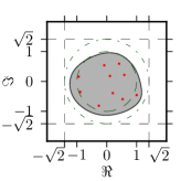
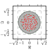
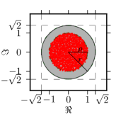
Figure 1. Spectrum (dots) and numerical range (dark convex set) of the complex Ginibre matrices of sizes $N=10,100$ and $1000$. The spectrum is asymptotically contained in the unit disk while numerical range converges to a disk of radius $r=\sqrt{2}$ denoted in the figures. Note the outer ring of the range is the non-normality belt of width $\sqrt{2}-1$ (it contains no eigenvalues).

Figure 2 shows analogous examples of diagonal matrices $D$ with the Ginibre spectrum – ensemble (4). Diagonal matrices are normal, so the numerical range equals to the support of the spectrum and thus converges to the unit disk. Note that this property hold also for a “normal Ginibre ensemble” of matrices of the kind $G^{\prime}=VDV^{*}$, where $D$ contains the spectrum of a Ginibre matrix, while $V$ is a random unitary matrix drawn according to the Haar measure.

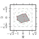
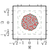
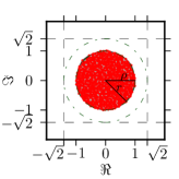
Figure 2. As in Fig. 1, for ensemble of diagonal matrices $D_{N}$ containing spectrum of Ginibre matrices of sizes $N=10,100$ and $1000$. Numerical range of these normal matrices coincides with the convex hull of their spectrum.

Analogous results for the upper triangular matrices $T$ of ensemble (3) shown in Fig.3. The numerical range asymptotically converges to the disk of radius $\sqrt{2}$ with probability one – see Theorem 4.2.

As all eigenvalues of $T$ are zero, the asymptotic properties of the spectrum and numerical range of $T$ become identical with these of a Jordan matrix $J$ of the same order $N$ rescaled by $\sqrt{2}$. By construction $J_{km}=1$ if $k+1=m$ and zero elsewhere for $k,m=1,\dots,N$. It is known [41] that numerical range of a Jordan matrix $J$ of size $N$ converges to the unit disk as $N\to\infty$.

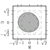
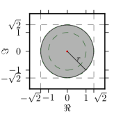
Figure 3. As in Fig. 1, for upper triangular random matrices $T_{N}$ of sizes $N=10,100$ and $1000$, for which all eigenvalues are equal to zero and the numerical range converges to the disk of radius $\sqrt{2}$.

In the table below we listed asymptotic predictions for the operator (spectral) norm $\|X\|$, the numerical radius $r(X)$, the spectral radius $\rho(X)$ and the squared non-normality parameter, $\bar{\mu}_{3}^{2}=\mathbb{E}(\mu_{3}^{2})$, of generic matrices pertaining to the ensembles investigated.

Ensemble	$\|X\|$	$r(X)$	$\rho(X)$	$\bar{\mu}^{2}_{3}(X)$
Ginibre $G$	$2$	$\sqrt{2}$	$1$	$N/2$
Diagonal $D$	$1$	$1$	$1$	$0$
Triangular $T$	$\sqrt{2e}$	$\sqrt{2}$	$0$	$N$

Consider a matrix $X$ of order $N$, normalized as Tr$XX^{*}=N$. Assume that the matrix is diagonal, so that its numerical range $W(X)$ is formed by the convex hull of the diagonal entries. Let us now modify the matrix $X$, writing $Y=\sqrt{1-a}X+\sqrt{a}T$, where $T$ is a strictly upper triangular random matrix normalized as above and $0\leq a\leq 1$. Note Tr$YY^{*}=N$ as well. Rescaling $X$ by a number $\sqrt{1-a}$ smaller than one and adding an off-diagonal part $\sqrt{a}T$ increases the non-normality belt of $Y$, i.e. the set $W(Y)\setminus\Gamma(Y)$. The larger relative weight of the off-diagonal part, the larger squared non-normality index, $\mu_{3}^{2}(Y)=\|Y\|^{2}_{\rm HS}-\sum_{i=1}^{N}|Y_{ii}|^{2}=N-(1-a)N=aN$ and the larger the non-normality belt of the numerical range. In the limiting case $a\to 1$ the off-diagonal part $\sqrt{a}T$ dominates the matrix $Y$. In particular, if $T=T_{N}$ of ensemble (3) then its numerical range converges to the disk of radius $\sqrt{2}$ as $N$ grows to infinity.

To demonstrate this construction in action we plotted in Fig. 4 numerical range of an exemplary random matrix $Y^{\prime}=D_{N}+\frac{1}{\sqrt{2}}T_{N}$, which contains the spectrum of the complex Ginibre matrix $G_{N}$ at the diagonal, and the matrix $T_{N}$ in its upper triangular part. The relative weight $a=1/\sqrt{2}$ is chosen in such a way that Tr$Y^{\prime}{Y^{\prime}}^{*}=N$. Thus $Y^{\prime}$ displays similar properties to the complex Ginibre matrix: its numerical range is close to a disk of radius $r=\sqrt{2}$, while the support of the spectrum is close to the unit disk. This observation is related to the fact [32] that bringing the complex Ginibre matrix by a unitary rotation to its triangular Schur form, $S:=UGU^{*}=D+T$, one assures that the diagonal matrix $D$ contains spectrum of $G$, while $T$ is an upper triangular matrix containing independent Gaussian random numbers.

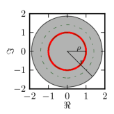
Figure 4. As in Fig. 1, for a) $D_{N}+\frac{1}{\sqrt{2}}T_{N}$ and b) $U_{N}+T_{N}$ of size $N=1000$.

Another illustration of the non-normality belt is presented in Fig. 4b. It shows the numerical range of the sum of a diagonal random unitary matrix $U_{N}$ of ensemble (5), with all eigenphases drawn independently according to a uniform distribution, with the upper triangular matrix $T_{N}$ of ensemble (3). All eigenvalues of this matrix belong to the unit circle, while presence of the triangular contribution increases the numerical radius $r$ and forms the non-normality belt. Some other examples of numerical range computed numerically for various ensembles of random matrices can be found in [36].

3. Some basic facts and notation

In this paper, $C_{0}$, $C_{1}$, …, $c_{1}$, $c_{2}$, … denote absolute positive constants, whose value can change from line to line. Given a square matrix $X$, we denote

$$\mbox{Re }X=\frac{X+X^{*}}{2}\quad\quad\mbox{ and }\quad\quad\mbox{Im }X=\frac{X-X^{*}}{2i},$$

so that $X=\mbox{Re }X+i\mbox{ Im }X$ and both $\mbox{Re }X$ and $\mbox{Im }X$ are self-adjoint matrices. Then it is easy to see that

$$\mbox{Re }W(X)=W(\mbox{Re }X)\quad\quad\mbox{ and }\quad\quad\mbox{Im }W(X)=W(\mbox{Im }X).$$

Given $\theta\in[0,2\pi]$, denote $X_{\theta}:=e^{i\theta}X$ and by $\lambda_{\theta}$ denote the maximal eigenvalue of $\mbox{Re }X_{\theta}$. It is known (see e.g. Theorem 1.5.12 in [23]) that

(4) $$W(X)=\bigcap_{0\leq\theta\leq 2\pi}H_{\theta},$$

where

$$H_{\theta}=e^{-i\theta}\left\{z\in{\mathbb{C}}\,:\,\mbox{Re }z\leq\lambda_{\theta}\right\}.$$

Our results for random matrices are somewhat similar, however we use the norm $\|X_{\theta}\|$ instead of its maximal eigenvalue. Repeating the proof of (4) (or adjusting the proof of Proposition 5.1 below), it is not difficult to see that

(5) $$W(X)\subset K(R),$$

where $K(R)$ is a star-shaped set defined by

(6) $$K(R):=\{\lambda e^{-i\theta}\,\|X_{\theta}\|\,\,:\,\,\lambda\in[0,1],\,\theta\in[0,2\pi)\}.$$

Below we provide a complete proof of corresponding results for random matrices. Note that $K(R)$ can be much larger than $W(X)$. Indeed, in the case of the identity operator $I$ the numerical range is a singleton, $W(I)=\{1\}$, while the set $K(R)$ is defined by the equation $\rho\leq|\cos t|$ (in the polar coordinates).

3.1. GUE

We say that a Hermitian $N\times N$ matrix $A=\{A_{i,j}\}_{i,j}$ pertains to Gaussian Unitary Ensemble (GUE) if a. its entries $A_{i,j}$’s are independent for $1\leq i\leq j\leq N$, b. the entries $A_{i,j}$’s for $1\leq i<j\leq N$ are complex centered Gaussian random variables of variance $1$ (that is the real and imaginary parts are independent centered Gaussian of variance $1/2$), c. the entries $A_{i,i}$’s for $1\leq i\leq N$ are real centered Gaussian random variables of variance $1$.

Clearly, for the complex Ginibre matrix $G_{N}$ its real part, $Y_{N}:=Re(G_{N})$, is a $(2N)^{-1/2}$ multiple of a GUE. It is known that with probability one $\|Y_{N}\|\to\sqrt{2}$ (see e.g. Theorem 5.2 in [7] or Theorem 5.3.1 in [35]). We will also need the following quantitative estimates. In [2, 27, 28, 30] it was shown that for GUE, normalized as $Y_{N}$, one has for every $\varepsilon\in(0,1]$,

$${\mathbb{P}}\left(\|Y_{N}\|\geq\sqrt{2}+\varepsilon\right)\leq C_{0}\exp(-c_{0}N\varepsilon^{3/2}).$$

Moreover, in [30] it was also shown that for $\varepsilon\in(0,1]$,

$${\mathbb{P}}\left(\|Y_{N}\|\leq\sqrt{2}-\varepsilon\right)\leq C_{1}\exp(-c_{1}N^{2}\varepsilon^{3}).$$

Note that $C_{1}\exp(-c_{1}N^{2}\varepsilon^{3})\leq C_{2}\exp(-c_{1}N\varepsilon^{3/2})$. Thus, for $\varepsilon\in(0,1]$,

(7) $${\mathbb{P}}\left(|\|Y_{N}\|-\sqrt{2}|>\varepsilon\right)\leq C_{3}\exp(-c_{2}N\varepsilon^{3/2})$$

(cf. Theorem 2.7 in [10]). It is also well known (and follows from concentration) that there exists two absolute constants $c_{4}$ and $C_{4}$ such that

(8) $${\mathbb{P}}\left(\|G_{N}\|\geq 2.1\right)\leq C_{4}\exp(-c_{4}N).$$

3.2. Upper triangular matrix

Let $g_{i}$, $h_{i}$, $i\geq 1$, be independent $\mathcal{N}(0,1)$ real random variables. It is well-known (and follows from the Laplace transform) that

$$\mathbb{E}\max_{i\leq N}|g_{i}|\leq\sqrt{2\ln(2N)}.$$

Since $\|x\|_{\infty}\leq\|x\|_{2}$, the classical Gaussian concentration inequality (see [9] or inequality (2.35) in [26]) implies that for every $r>0$,

(9) $${\mathbb{P}}\left(\max_{i\leq N}|g_{i}|>\sqrt{2\ln(2N)}+r\right)\leq e^{-r^{2}/2}.$$

Recall that $T_{N}$ denotes the upper triangular $N\times N$ Gaussian random matrix normalized such that $\mathbb{E}T_{N}T_{N}^{*}=N$, that is $(T_{N})_{ij}$ are independent complex Gaussian random variables of variance $2/(N-1)$ for $1\leq i<j\leq N$ and $0$ otherwise. Note that $\mbox{Re }T_{N}$ can be presented as $Z_{N}/\sqrt{2(N-1)}$, where $Z_{N}$ is a complex Hermitian $N\times N$ matrix with zero on the diagonal and independent complex Gaussian random variables of variance one above the diagonal. Let $A_{N}$ be distributed as GUE (with $g_{i}$’s on the diagonal) and $V_{N}$ be the diagonal matrix with the same diagonal as $A_{N}$. Clearly, $Z_{N}=A_{N}-V_{N}$. Therefore, the triangle inequality and (7) yield that for every $\varepsilon\in(0,1]$

(10) $${\mathbb{P}}\left(\left|\frac{1}{\sqrt{N}}\|Z_{N}\|-2\right|>\varepsilon\right)\leq C\exp(-cN\varepsilon^{3/2}),$$

where $C$ and $c$ are absolute positive constants (formally, applying the triangle inequality, we should ask $\varepsilon>\sqrt{\ln(2N)/N}$, but if $\varepsilon\leq\sqrt{\ln(2N)/N}$ the right hand side becomes large than 1, by an appropriate choice of the constant $C$). In particular, the Borel-Cantelli lemma implies that with probability one $\|Z_{N}\|/\sqrt{N}\to 2$ (alternatively one can apply Theorem 5.2 from [7]).

4. Main results

Our first main result is

Theorem 4.1.

Let $R>0$. Let $\{X_{N}\}_{N}$ be a sequence of complex random $N\times N$ matrices such that for every $\theta\in{\mathbb{R}}$ with probability one

$$\lim_{N\to\infty}\|\mbox{\rm Re }(e^{i\theta}X_{N})\|=R.$$

Then with probability one

$$\lim_{N\to\infty}d_{H}\left(W(X_{N}),D(0,R)\right)=0.$$

Furthermore, if there exists $A\geq\max\{R,1\}$ such that for every $N\geq 1$,

$${\mathbb{P}}\left(\|X_{N}\|>A\right)\leq p_{N}$$

and for every $\varepsilon\in(0,1/2)$, $N\geq 1$, $\theta\in{\mathbb{R}}$,

$${\mathbb{P}}\left(\left|\,\|\mbox{\rm Re }(e^{i\theta}X_{N})\|-R\right|>\varepsilon\right)\leq q_{N}(\varepsilon)$$

then for every positive $\varepsilon\leq\min\{1/2,\sqrt{R/(A+1)}\}$ and every $N$ one has

$${\mathbb{P}}\left(d_{H}(W(X_{N}),D(0,R)>4A\varepsilon\right)\leq p_{N}+7R\varepsilon^{-2}\ q_{N}(\varepsilon^{2}).$$

Proof.

Fix positive $\varepsilon\leq\min\{1/2,R/(A+1)\}$. Since the real part of a matrix is a self-adjoint operator we have

$$\lambda(\theta,N):=\|\mbox{Re }(e^{i\theta}X_{N})\|=\sup\{\mbox{Re }(e^{i\theta}X_{N}y,y)\,:\,\|y\|_{2}=1\}.$$

By assumptions of the theorem, for every $\theta\in{\mathbb{R}}$ with probability one

$$\lim_{N\to\infty}\lambda(\theta,N)=R.$$

Let ${\mathbb{S}}$ denote the boundary of the disc $D(0,R)$. Choose a finite $\varepsilon$-net $\mathcal{N}$ in $[0,2\pi]$, so that $\{Re^{i\theta}\}_{\theta\in{\mathcal{N}}}$ is an $\varepsilon$-net (in the geodesic metric) in ${\mathbb{S}}$. Then, with probability one, for every $\theta\in{\mathcal{N}}$ one has $\lambda(\theta,N)\to R$.

Since $\mbox{Im }X_{N}=\mbox{Re }(e^{-i\pi/2}X_{N})$, one has

$$R\leq\limsup_{N\to\infty}\|X_{N}\|\leq\limsup_{N\to\infty}\|\mbox{Re }X_{N}\|+\limsup_{N\to\infty}\|\mbox{Im }X_{N}\|=2R.$$

Choose $A\geq\max\{R,1\}$ and $N\geq 1$ such that for every $M\geq N$ one has

$$\|X_{M}\|\leq A\quad\mbox{ and }\quad\forall\theta\in{\mathcal{N}}\,\,\,\,|\lambda(\theta,M)-R|\leq\varepsilon.$$

Fix $M\geq N$. Note that the supremum in the definition of $\lambda(\theta,M)$ is attained and that

$$|\mbox{Re }(e^{i\theta}X_{M}y,y)-\mbox{Re }(e^{it}X_{M}y,y)|\leq|e^{i\theta}-e^{it}|\cdot|(X_{M}y,y)|\leq\varepsilon A,$$

whenever $|\theta-t|\leq\varepsilon$ and $\|y\|_{2}=1$. Using approximation by elements of $\mathcal{N}$, we obtain for every real $t$,

$$|\lambda(t,M)-R|\leq(A+1)\varepsilon.$$

Let $y_{0}$ be such that $\|y_{0}\|=1$ and

$$\lambda:=\sup\{|(X_{M}y,y)|\,:\,||y||_{2}=1\}=|(X_{M}y_{0},y_{0})|.$$

Then for some $t$

$$\lambda=e^{it}(X_{M}y_{0},y_{0})=\mbox{Re }(e^{it}X_{M}y_{0},y_{0})=\lambda(t,M)\leq R+(A+1)\varepsilon.$$

This shows that $W(X_{M})\subset D(0,R+(A+1)\varepsilon)$.

Finally fix some $z\in{\mathbb{S}}$, that is $z=Re^{it}$. Choose $\theta\in{\mathcal{N}}$ such that $|t-\theta|\leq\varepsilon$. Let $y_{1}$ be such that

$$\lambda(-\theta,M)=\mbox{Re }(e^{-i\theta}X_{M}y_{1},y_{1})=\mbox{Re }(e^{-i\theta}(X_{M}y_{1},y_{1})).$$

Denote $x:=(X_{N}y_{1},y_{1})$. Then

$$R-(A+1)\varepsilon\leq\mbox{Re }(e^{-i\theta}x)\leq|x|\leq R+(A+1)\varepsilon.$$

Since $A\geq\max\{R,1\}$ and $\varepsilon\leq R/(A+1)$, this implies that

$$|Re^{i\theta}-x|\leq\sqrt{(A+1)^{2}\varepsilon^{2}+4R(A+1)\varepsilon}\leq 2A\sqrt{\varepsilon}\,\sqrt{\varepsilon+2}.$$

Since $|t-\theta|\leq\varepsilon$ and $\varepsilon<1/2$, we observe that

$$|z-x|\leq R|e^{it}-e^{i\theta}|+|Re^{i\theta}-x|\leq R\varepsilon+2\sqrt{2.5}A\sqrt{\varepsilon}\leq 4A\sqrt{\varepsilon}.$$

Therefore, for every $z\in{\mathbb{S}}$ there exists $x\in W(X_{M})$ with

$$|z-x|\leq 4A\sqrt{\varepsilon}.$$

Using convexity of $W(X_{M})$, we obtain that with probability one

$$d_{H}(W(X_{M}),D(0,R))\leq 4A\sqrt{\varepsilon}.$$

Since $M\geq N$ was arbitrary, this implies the desired result.

The proof of the second part of the theorem is essentially the same. Note that the $\varepsilon$-net in our proof can be chosen to have the cardinality not exceeding $2.2\pi R/\varepsilon$. Thus, by the union bound, the probability of the event

$$\|X_{M}\|\leq A\quad\mbox{ and }\quad\forall\theta\in{\mathcal{N}}\,\,\,\,|\lambda(\theta,M)-R|\leq\varepsilon,$$

considered above, does not exceed $p_{N}+2.2\pi R\ \varepsilon^{-1}q_{N}(\varepsilon).$ This implies the quantitative part of the theorem. ∎

The next theorem shows that the first part of Theorem 4.1 applies to a large class of random matrices (essentially to matrices whose entries are i.i.d. random variables having final fourth moments and corresponding triangular matrices), in particular to ensembles $G_{N}$, $G^{{\mathbb{R}}}_{N}$ and $T_{N}$ introduced in Section 2.

Theorem 4.2.

Let $x_{i,i}$, $i\geq 1$, be i.i.d. complex random variables with finite second moment, $x_{i,j}$, $i\neq j$, be i.i.d. centered complex random variables with finite fourth moment, and all these variables are independent. Assume ${\mathbb{E}}|x_{1,2}|^{2}=\lambda^{2}$ for some $\lambda>0$. Let $X_{N}=N^{-1/2}\,\{x_{i,j}\}_{i,j\leq N},$ and $Y_{N}$ be the matrix whose entries on or above the diagonal are the same as entries of $X_{N}$ and entries below diagonal are zeros. Then with probability one,

$$d_{H}(W(X_{N}),D(0,\sqrt{2}\lambda))\to 0\quad\mbox{ and }\quad d_{H}(W(Y_{N}),D(0,\lambda))\to 0.$$

In particular with probability one,

$$d_{H}(W(G_{N}),D(0,\sqrt{2}))\to 0,\quad d_{H}(W(G^{{\mathbb{R}}}_{N}),D(0,\sqrt{2}))\to 0$$

and

$$d_{H}(W(T_{N}),D(0,\sqrt{2}))\to 0.$$

Proof.

It is easy to check that the entries of $\sqrt{N}\,Re(e^{i\theta}X_{N})$ satisfy conditions of Theorem 5.2 in [7], that is the diagonal entries are i.i.d. real random variables with finite second moment; the above diagonal entries are i.i.d. mean zero complex variables with finite fourth moment and of variance $\lambda^{2}/2$. Therefore, Theorem 5.2 in [7] implies that $\|Re(e^{i\theta}X_{N})\|\to\sqrt{2}\lambda$. Theorem 4.1 applied with $R=\sqrt{2}\lambda$ provides the first limit. For the triangular matrix $Y_{N}$ the proof is the same, we just need to note that the above diagonal entries of $\sqrt{N}\,Re(e^{i\theta}Y_{N})$ have variances $(\lambda/2)^{2}$. The “in particular” part follows immediately. ∎

We now turn to quantitative estimates for ensembles $G_{N}$ and $T_{N}$.

Theorem 4.3.

There exist absolute positive constants $c$ and $C$ such that for every $\varepsilon\in(0,1]$ and every $N$,

$${\mathbb{P}}\left(d_{H}\left(W(G_{N}),D(0,\sqrt{2})\right)\geq\varepsilon\right)\leq C\ \varepsilon^{-2}\ \exp(-cN\varepsilon^{3}).$$

Remark 1. Note that by Borel-Cantelli lemma, this theorem also implies that $d_{H}(W(G_{N}),D(0,\sqrt{2}))\to 0$.

Proof.

Note that for every real $\theta$ the distributions of $G_{N}$ and $e^{i\theta}G_{N}$ coincide. Note also that $\mbox{Re }(G_{N})$ is a $1/\sqrt{2N}$ multiple of a GUE. Thus, the desired result follows from the quantitative part of Theorem 4.1 by (7) and (8) (and by adjusting absolute constants). ∎

Remark 2. It is possible to establish a direct link between Theorem 4.3, geometry of the set of mixed quantum states and the Dvoretzky theorem [11, 33].

As before, let ${Q}_{N}=\{\varrho:\varrho=\varrho^{*},\ \varrho\geq 0,\ {\rm Tr}\varrho=1\}$ be the set of complex density matrices of size $N$. It is well known [8] that working in the geometry induced by the Hilbert-Schmidt distance this set of (real) dimension $N^{2}-1$ is inscribed inside a sphere of radius $\sqrt{(N-1)/N}\approx 1$, and it contains a ball of radius $1/\sqrt{(N-1)N}\approx 1/N$. Applying the Dvoretzky theorem and the techniques of [4], one can prove the following result [5]: for large $N$ a generic two-dimensional projection of the set ${Q}_{N}$ is very close to the Euclidean disk of radius $r_{N}=2/\sqrt{N}$. Loosely speaking, in high dimensions a typical projection of a convex body becomes close to a circular disk – see e.g. [3].

To demonstrate a relation with the numerical range of random matrices we apply results from [12], where it was shown that for any matrix $X$ of order $N$ its numerical range $W(X)$ is up to a translation and dilation equal to an orthogonal projection of the set ${Q}_{N}$. The matrix $X$ determines the projection plane, while the scaling factor for a traceless matrix reads $\alpha(X)=\sqrt{\frac{1}{2}({\rm Tr}XX^{*}+|{\rm Tr}X^{2}|)}$.

Complex Ginibre matrices are asymptotically traceless, and the second term $|{\rm Tr}G^{2}|$ tends to zero, so the normalization condition used in this work, ${\mathbb{E}}{\rm Tr}G_{N}G_{N}^{*}=N$, implies that ${\mathbb{E}}\alpha(G_{N})$ converges asymptotically to $\sqrt{N/2}$. It is natural to expect that the projection of ${Q}_{N}$ associated with the complex Ginibre matrix $G_{N}$ is generic and is characterized by the Dvoretzky theorem.

Our result shows that the random projection of ${Q}_{N}$, associated with the complex Ginibre matrix $G_{N}$ does indeed have the features expected in view of Dvoretzky’s theorem and is close to a disk of radius $r_{N}{\mathbb{E}}\alpha(G_{N})=\sqrt{2}$.

Theorem 4.4.

There exist absolute positive constants $c$ and $C$ such that for every $\varepsilon\in(0,1]$ and every $N$,

$${\mathbb{P}}\left(d_{H}\left(W(T_{N}),D(0,\sqrt{2})\right)\geq\varepsilon\right)\leq C\ \varepsilon^{-2}\ \exp(-cN\varepsilon^{3}).$$

Remark 3. Note that by Borel-Cantelli lemma, this theorem also implies that $d_{H}(W(T_{N}),D(0,\sqrt{2}))\to 0$.

Proof.

Note that for every real $\theta$ the distributions of $T_{N}$ and $e^{i\theta}T_{N}$ coincide. As was mentioned above $\mbox{Re }T_{N}$ can be presented as $Z_{N}/\sqrt{2(N-1)}$, where $Z_{N}$ is a complex Hermitian $N\times N$ matrix with zero on the diagonal and independent complex Gaussian random variables of variance one above the diagonal. Thus, by (10), for every $\theta\in{\mathbb{R}}$ and $\varepsilon\in(0,1]$

$${\mathbb{P}}\left(\left|\|\mbox{Re }(e^{i\theta}T_{N})\|-\sqrt{2}\right|>\varepsilon\right)\leq C\exp(-cN\varepsilon^{3/2})$$

(one needs to adjust the absolute constants). Since $X_{N}=\mbox{Re }X_{N}+i\mbox{Im }X_{N}=\mbox{Re }X_{N}+i\mbox{Re }(e^{-i\pi/2}X_{N})$,

$${\mathbb{P}}\left(\|T_{N}\|\geq 3\right)\leq C_{2}\exp(-c_{1}N).$$

Thus, applying Theorem 4.1 (with $R=\sqrt{2}$ and $A=3$), we obtain the desired result. ∎

5. Further extensions.

Note that the first part of the proof of Theorem 4.1, the inclusion of $W(X_{N})$ into the disk, can be extended to a more general setting, when $R$ is not a constant but a function of $\theta$. Namely, let $R:{\mathbb{R}}\to[1,\infty)$ be a $(2\pi)$-periodic continuous function. Let $K(R)$ be defined by (6), i.e.

$$K(R):=\{\lambda e^{-i\theta}\,R(\theta)\,\,:\,\,\lambda\in[0,1],\,\theta\in[0,2\pi)\}.$$

Note that if we identify ${\mathbb{C}}$ with ${\mathbb{R}}^{2}$ and $\theta$ with the direction $e^{-i\theta}$ then $R$ becomes the radial function of the star-shaped body $K(R)$. Then we have the following

Theorem 5.1.

Let $K(R)$ be a star-shaped body with a continuous radial function $R(\theta)$, $\theta\in[0,2\pi)$. Let $\{X_{N}\}_{N}$ be a sequence of complex random $N\times N$ matrices such that for every $\theta\in[0,2\pi)$ with probability one

$$\lim_{N\to\infty}\|\mbox{\rm Re }(e^{i\theta}X_{N})\|=R(\theta).$$

Then with probability one

$$\lim_{N\to\infty}d_{H}(W(X_{N})\setminus K(R),\emptyset)=0$$

(in other words asymptotically the numerical range is contained in $K(R)$). Furthermore, if there exists $A>0$ such that for every $N\geq 1$,

$${\mathbb{P}}\left(\|X_{N}\|>A\right)\leq p_{N}$$

and for every $\varepsilon\in(0,1/2)$, $N\geq 1$, $\theta\in{\mathbb{R}}$,

$${\mathbb{P}}\left(\left|\,\|\mbox{\rm Re }(e^{i\theta}X_{N})\|-R(\theta)\right|>\varepsilon\right)\leq q_{N}(\varepsilon)$$

then for every $\varepsilon\in(0,1/2)$ and every $N$ one has

$${\mathbb{P}}\left(d_{H}(W(X_{N})\subset K(R+(2A+1)\varepsilon)\right)\leq p_{N}+2L\varepsilon^{-1}\ q_{N}(\varepsilon),$$

where $L$ denotes the length of the curve $\{R(\theta)\}_{\theta\in[0,2\pi)}$.

Remark 4. The proof below can be adjusted to prove the inclusion (5) (in fact (5) is simpler, since it does not require the approximation).

Remark 5. Under assumptions of Proposition 5.1 on the convergence of norms to $R$, the function $R$ must be continuous. Indeed, for every $\theta$ and $t$ one has with probability one

$$|R(\theta)-R(t)|\leq\lim_{N\to\infty}\left|\,\|\mbox{Re }(e^{i\theta}X_{N})\|-\|\mbox{Re }(e^{it}X_{N})\|\right|$$

$$\leq\left|e^{i\theta}-e^{it}\right|\limsup_{N\to\infty}\|X_{N}\|$$

and

$$\limsup_{N\to\infty}\|X_{N}\|\leq\limsup_{N\to\infty}\|\mbox{Re }X_{N}\|+\limsup_{N\to\infty}\|\mbox{Im }X_{N}\|=R(0)+R(-\pi/2).$$

Remark 6. Continuity and periodicity are not the only constraints that $R$ should satisfy. For Theorem 5.1 not to be an empty statement, The set $K(R)$ should also have the property of being convex. This is clearly a necessary condition, and it can be proved by simple diagonal examples that it is also a sufficient condition.

Proof. Fix $\varepsilon\in(0,1/2)$. Denote

$$\lambda(\theta,N):=\sup\{\mbox{Re }(e^{i\theta}X_{N}y,y),\|y\|_{2}=1\}.$$

Note that

$$\lambda(\theta,N)=\|\mbox{Re }(e^{i\theta}X_{N})\|.$$

Thus for every $\theta\in{\mathbb{R}}$ with probability one

$$\lim_{N\to\infty}\lambda(\theta,N)=R(\theta).$$

Let $\partial K=\{R(\theta)\,\mid\,\theta\in[0,2\pi)\}$ denote the boundary of $K(R)$. Choose a finite set $\mathcal{N}$ in $[0,2\pi]$ so that $\{R(\theta)e^{i\theta}\}_{\theta\in\mathcal{N}}$ is an $\varepsilon$-net in $\partial K$ (in the Euclidean metric). Then, with probability one, for every $\theta\in{\mathcal{N}}$ one has $\lambda(\theta,N)\to R(\theta)$.

As before, note

$$\max_{\theta}R(\theta)\leq\limsup_{N\to\infty}\|X_{N}\|\leq R(0)+R(-\pi/2).$$

Choose $A\geq 1$ and $N\geq 1$ such that for every $M\geq N$ one has

$$\|X_{M}\|\leq A\quad\mbox{ and }\quad\forall\theta\in{\mathcal{N}}\,\,\,\,|\lambda(\theta,M)-R(\theta)|\leq\varepsilon.$$

Note that the supremum in the definition of $\lambda(\theta,N)$ is attained and that

$$|e^{i\theta}-e^{it}|\,\|X_{N}\|\leq|e^{i\theta}-e^{it}|\,A,$$

whenever $\|y\|_{2}=1$. As was mentioned in the remark following the theorem,

$$|R(\theta)-R(t)|\leq\left|e^{i\theta}-e^{it}\right|A.$$

Therefore, using approximation by elements of $\mathcal{N}$ and the simple estimate $\left|e^{i\theta}-e^{it}\right|\leq\varepsilon$, whenever $|\theta-t|\leq\varepsilon$, we obtain that for every real $t$ one has

$$|\lambda(t,N)-R(t)|$$

$$\leq|\lambda(t,N)-\lambda(\theta,N)|+|\lambda(\theta,N)-R(\theta)|+|R(\theta)-R(t)|$$

(11) $$\leq(2A+1)\varepsilon.$$

Now let $y_{0}$ of norm one be such that $(X_{N}y_{0},y_{0})$ is in the direction $e^{it}$, that is $(X_{N}y_{0},y_{0})=e^{it}R$ for some real positive $R$. Then

$$R=e^{-it}(X_{N}y_{0},y_{0})=\mbox{Re }(e^{-it}X_{N}y_{0},y_{0})\leq\lambda(-t,N)\leq R(-t)+(2A+1)\varepsilon.$$

This shows that $W(X_{N})\subset K(R+(2A+1)\varepsilon)$.

The quantitative estimates are obtained in the same way as in the proof of Theorem 4.1. ∎

As an example consider the following matrix. Let $H_{1}$, $H_{2}$ be independent distributed as $G_{N}$, $a,b>0$ and $A:=aH_{1}+ibH_{2}$. Then it is easy to see that $\mbox{Re }(e^{i\theta}A)$ is distributed as $r(\theta)G_{N}$, where $r(\theta)=\sqrt{a^{2}\cos^{2}\theta+b^{2}\sin^{2}\theta}$. Therefore $\|\mbox{Re }(e^{i\theta}A)\|\to R(\theta):=\sqrt{2}r(\theta)$. Theorem 5.1 implies that $W(A)$ is asymptotically contained in $K(R)$ which is an ellipse.

6. Norm estimate for the upper triangular matrix

In this section we prove that $\|T_{N}\|\to\sqrt{2e}$, as claimed in Eq. (2) of the introduction (Theorem 6.2). For the purpose of this section it is convenient to renormalize the matrix $T_{N}$ and to consider $\bar{T}_{N}$, which is strictly upper diagonal and whose entries above the diagonal are complex centered i.i.d. Gaussians of variance $1/\sqrt{N}$. Thus, $(\bar{T}_{N})_{ij}=\sqrt{(N-1)/(2N)}T_{ij}$.

We also consider upper triangular matrices $T_{N}^{\prime}$, whose entries above and on the diagonal are complex centered i.i.d. Gaussians of variance $1/\sqrt{N}$. Note that $\bar{T}_{N}$ and $T_{N}^{\prime}$ differs on the diagonal only, therefore the following lemma follows from (9).

Lemma 6.1.

The operator norm of $\bar{T}_{N}$ converges with probability one to a limit $L$ iff the operator norm of $T_{N}^{\prime}$ converges with probability one to $L$.

We reformulate the limiting behavior of $\|T_{N}\|$ in terms of $\bar{T}_{N}$. We prove the following theorem, which is clearly equivalent to (2).

Theorem 6.2.

With probability one, the operator norm of the sequence of random matrices $\bar{T}_{N}$ tends to $\sqrt{e}$.

Let us first recall the following theorem, proved in [13].

Proposition 6.3.

For any integer $\ell$,

$$\lim_{N}{\mathbb{E}}(N^{-1}Tr((\bar{T}_{N}\bar{T}_{N}^{*})^{\ell})=\frac{\ell^{\ell}}{(\ell+1)!}$$

We will use the following auxiliary constructions. Fix a positive integer parameter $k$, denote $m=[N/k]$ (the largest integer not exceeding $N/k$), and define the upper triangular matrix $\bar{T}_{N,k}$ as follows: $(\bar{T}_{N,k})_{i,j}=0$ if $\ell m+1\leq j\leq(\ell+1)m$ and $i\geq\ell m+1$ for some $\ell\geq 0$, and $(\bar{T}_{N,k})_{i,j}=(\bar{T}_{N})_{i,j}$ otherwise. In other words we set more entries to be equal to 0 and we have either $k\times k$ or $(k+1)\times(k+1)$ block strictly triangular matrix (if $N$ is not multiple of $k$ then the last, $(k+1)$th, “block-row” and “block-column” have either their number of rows or columns strictly less than $N/k$).

We start with the following

Lemma 6.4.

Let $k$ be a positive integer and $N$ be a multiple of $k$. Then with probability one, $\|\bar{T}_{N,k}\|$ converges to a quantity $f_{k}$ as $N\to\infty$.

Proof.

Note that the complex Ginibre matrix is, up to a proper normalization, distributed as $A_{1}+iA_{2}$, where $A_{1}$ and $A_{2}$ are i.i.d. GUE. Thus, when $N$ is a multiple of $k$, $\bar{T}_{N,k}$ can be seen as a $k\times k$ block matrix of $N/k\times N/k$ matrices, which are linear combinations of i.i.d. copies of GUE. A Haagerup-Thorbjornsen result [21] ensures convergence with probability one of the norm. ∎

At this point it is not possible to compute $f_{k}$ explicitly. Actually it will be enough for us to understand the asymptotics of $f_{k}$ as $k\to\infty$.

In the next lemma, we remove the condition that $N$ be a multiple of $k$.

Lemma 6.5.

Let $k$ be a positive integer. Then with probability one, $\|\bar{T}_{N,k}\|$ converges to to the quantity $f_{k}$ defined in Lemma 6.4 as $N\to\infty$.

Proof.

Let $N\geq k$. Denote by $N_{+}$ the first multiple of $k$ after $N$. Up to an overall multiple $N/N_{+}$ (imposed by the normalization that is dimension dependent), we can realize $\bar{T}_{N,k}$ as a compression of $\bar{T}_{N_{+},k}$. Since a compression reduces the operator norm, thanks to the previous lemma, we have with probability one,

$$\limsup_{N\to\infty}\|\bar{T}_{N,k}\|\leq f_{k}.$$

Similarly, by $N_{-}$ denote the first multiple of $k$ before $N$. Up to an overall multiple $N_{-}/N$, we can realize $\bar{T}_{N_{-},k}$ as a compression of $\bar{T}_{N,k}$. Therefore we have with probability one,

$$\liminf_{N\to\infty}\|\bar{T}_{N,k}\|\geq f_{k}.$$

These two estimates imply the lemma. ∎

In the next Lemma, we compare the norm of $\bar{T}_{N,k}$ with the norm of $\bar{T}_{N}$.

Lemma 6.6.

With probability one for every $k$ we have

$$\limsup_{N\to\infty}\left|\|\bar{T}_{N,k}\|-\|\bar{T}_{N}\|\right|\leq 3/\sqrt{k}.$$

Proof.

For every fixed $k\leq N$ we consider a matrix $D_{N,k}$ distributed as $\bar{T}_{N,k}-\bar{T}_{N}$. Setting as before $m=[N/k]$, the entries of $D_{N,k}$ are i.i.d. Gaussian of variance $1/\sqrt{N}$ if $\ell m+1\leq j\leq(\ell+1)m$ and $i\geq\ell m+1$ for some $\ell\geq 0$, and $(D_{N,k})_{i,j}=0$ otherwise. Clearly, this matrix is diagonal by block. It consists of $k$ diagonal blocks of $m\times m$ strictly upper triangular random matrices with entries of variance $1/N$ and possibly one more block of smaller size.

Let us first work on estimating the tail of the operator norm on a diagonal block of size $m\times m$, which will be denoted by $X_{N}$. It follows directly from the Wick formula that the quantities ${\mathbb{E}}(Tr((X_{N}X_{N}^{*})^{\ell}))$ are bounded above by quantities ${\mathbb{E}}(Tr((\tilde{X}_{N}\tilde{X}_{N}^{*})^{\ell}))$, where $\tilde{X}_{N}$ is the same matrix as $X_{N}$ without the assumption that lower triangular entries are zero (in other words, it is a rescaled complex Ginibre matrix of size $m\times m$). From there, we can make estimates following arguments à la Soshnikov [37] and obtain that the tail of the operator norm of $X_{N}$ is majorized by the tail of the operator norm of $\tilde{X}_{N}$. More precisely, we can show that there exists a constant $C_{1}>0$ such that ${\mathbb{E}}(Tr((X_{N}X_{N}^{*})^{\ell}))\leq C_{1}(2.8/\sqrt{k})^{\ell}$ for every $\ell\leq N^{1/4}$. This implies that there exists another constant $C_{2}>0$ such that ${\mathbb{E}}(Tr(D_{N,k}^{\ell}))\leq C_{1}k(2.8/\sqrt{k})^{\ell}\leq C_{2}(2.9/\sqrt{k})^{\ell}$ for all sufficiently large $\ell\leq N^{1/4}$. Therefore we deduce by Jensen inequality that the probability that the operator norm $D_{N,k}$ is larger than $3/\sqrt{k}$ is bounded by $C^{-N}$ for some universal constant $C>1$. By Borel-Cantelli lemma, with probability one we have

$$\limsup_{N\to\infty}\left|\|\bar{T}_{N,k}\|-\|\bar{T}_{N}\|\right|\leq 3/\sqrt{k}.$$

The result follows by the triangle inequality. ∎

As a consequence we obtain the following lemma.

Lemma 6.7.

The sequence $f_{k}$ converges to some constant $f$ as $k\to\infty$ and $\|\bar{T}_{N}\|$ converges to $f$ with probability one.

Proof.

By Lemma 6.6 and the triangle inequality, we get that with probability one,

$$\limsup_{N\to\infty}\left|\|\bar{T}_{N,k_{1}}\|-\|\bar{T}_{N,k_{2}}\|\right|\leq 3/\sqrt{k_{1}}+3/\sqrt{k_{2}}.$$

Therefore, evaluating the limit on the left hand side, we observe that $\{f_{k}\}_{k}$ is a Cauchy sequence. Thus it converges to a constant $f$.

Next, we see that for any $\varepsilon>0$, taking $k$ large enough, we obtain that with probability one,

$$\limsup_{N\to\infty}\left|\|\bar{T}_{N}\|-f\right|\leq\varepsilon.$$

Letting $\varepsilon\to 0$, we obtain the desired result. ∎

Now we are ready to finish the proof of Theorem 6.2.

Proof of Theorem 6.2.

It is enough to prove that $f=\sqrt{e}$. It follows from [21] that

$$f_{k}=\lim_{\ell\to\infty}\sqrt[2\ell]{\lim_{N\to\infty}{\mathbb{E}}(N^{-1}Tr((\bar{T}_{N,k}\bar{T}_{N,k}^{*})^{\ell}))}.$$

Given $\ell$ and $N$, it follows from Wick’s theorem that ${\mathbb{E}}(N^{-1}Tr((\bar{T}_{N,k}\bar{T}_{N,k}^{*})^{\ell}))$ increases and converges as $k\to\infty$ pointwisely to ${\mathbb{E}}(N^{-1}Tr((\bar{T}_{N}\bar{T}_{N}^{*})^{\ell}))$. So the same result holds if we let $N\to\infty$ (by Dini’s theorem), namely

$$\lim_{k\to\infty}\lim_{N\to\infty}{\mathbb{E}}(N^{-1}Tr((\bar{T}_{N,k}\bar{T}_{N,k}^{*})^{\ell}))=\lim_{N\to\infty}{\mathbb{E}}(N^{-1}Tr((\bar{T}_{N}\bar{T}_{N}^{*})^{\ell})).$$

Observing that

$$\sqrt[2\ell]{\lim_{N}{\mathbb{E}}(N^{-1}Tr((\bar{T}_{N,k}\bar{T}_{N,k}^{*})^{\ell}))}$$

increases as a function of $\ell$ and applying once more Dini’s theorem, we obtain that

$$\lim_{k\to\infty}f_{k}=\lim_{\ell\to\infty}\sqrt[2\ell]{\lim_{N\to\infty}{\mathbb{E}}(N^{-1}Tr((\bar{T}_{N}\bar{T}_{N}^{*})^{\ell}))}.$$

Therefore

$$\lim_{k\to\infty}f_{k}=\lim_{\ell\to\infty}\sqrt[2\ell]{\frac{\ell^{\ell}}{(\ell+1)!}}=\sqrt{e}$$

by the Stirling formula. This completes the proof. ∎

Acknowledgment. We are grateful to Guillaume Aubrun and Stanisław Szarek for fruitful discussions on the geometry of the set of quantum states, helpful remarks, and for letting us know about their results prior to publication. It is also a pleasure to thank Zbigniew Puchała and Piotr Śniady for useful comments. Finally we would like to thank an anonymous referee for careful reading and valuable remarks which have helped us to improve the presentation.

References

- [1] G. W. Anderson, A. Guionnet, O. Zeitouni, An introduction to random matrices, Cambridge Studies in Advanced Mathematics, 118. Cambridge University Press, Cambridge, 2010.
- [2] G. Aubrun, A sharp small deviation inequality for the largest eigenvalue of a random matrix, Seminaire de Probabilites XXXVIII, 320–337, Lecture Notes in Math., 1857, Springer, Berlin, 2005.
- [3] G. Aubrun and J. Leys, Quand les cubes deviennent ronds, http://images.math.cnrs.fr/Quand-les-cubes-deviennent-ronds.html
- [4] G. Aubrun, S. J. Szarek, Tensor products of convex sets and the volume of separable states on qudits, Phys. Rev. A 73 022109 (2006).
- [5] G. Aubrun, S. J. Szarek, private communication
- [6] Z. D. Bai, Circular law, Ann. Probab. 25 (1997), 494–529.
- [7] Z. D. Bai, J. W. Silverstein, Spectral analysis of large dimensional random matrices. Second edition. Springer Series in Statistics. Springer, New York, 2010.
- [8] I. Bengtsson and K. Życzkowski, Geometry of Quantum States, Cambridge University Press, Cambridge, 2006.
- [9] B. S. Cirel’son, I. A. Ibragimov, V. N. Sudakov, Norms of Gaussian sample functions, Proc. 3rd Japan-USSR Symp. Probab. Theory, Taschkent 1975, Lect. Notes Math. 550 (1976), 20–41.
- [10] K. R. Davidson, S. J. Szarek, Local operator theory, random matrices and Banach spaces, Handbook of the geometry of Banach spaces, Vol. I, 317–366, North-Holland, Amsterdam, 2001.
- [11] A. Dvoretzky, Some results on convex bodies and Banach spaces, Proc. Internat. Sympos. Linear Spaces, Jerusalem 1960; p. 123–160 (1961).
- [12] C. F. Dunkl, P. Gawron, J. A. Holbrook, J. Miszczak, Z. Puchała, K. Życzkowski, Numerical shadow and geometry of quantum states, J. Phys. A 44 (2011) 335301 (19 pp.)
- [13] K. Dykema, U. Haagerup, DT-operators and decomposability of Voiculescu’s circular operator, Amer. J. Math. 126 (2004), 121–189.
- [14] L. Elsner and M. H. C. Paardekooper, On measures of nonnormality of matrices, Lin. Alg. Appl. 92, 107–124 (1987).
- [15] S. Geman, A limit theorem for the norm of random matrices, Ann. Probab. 8 (1980), 252–261.
- [16] J. Ginibre, Statistical ensembles of complex, quaternion, and real matrices, J. Math. Phys. 6 (1965), 440–449.
- [17] V. L. Girko, The circular law, Teor. Veroyatnost. i Primenen. 29 (1984), 669–679.
- [18] F. Götze, A. Tikhomirov, The circular law for random matrices, Ann. Probab. 38 (2010), 1444–1491.
- [19] K. E. Gustafson and D. K. M. Rao, Numerical Range: The Field of Values of Linear Operators and Matrices. Springer-Verlag, New York, 1997.
- [20] U. Haagerup and S. Thorbjørnsen, Random matrices with complex Gaussian entries. Expositiones Math. 21 (2003), 293–337.
- [21] U. Haagerup, S. Thorbjørnsen, A new application of random matrices: is not a group, Ann. of Math. 162 (2005), 711–775.
- [22] F. Hausdorff, Der Wertevorrat einer Bilinearform, Math. Zeitschrift 3 (1919), 314–316.
- [23] R. A. Horn and C. R. Johnson, Topics in Matrix Analysis, Cambridge University Press, Cambridge, 1994.
- [24] C. R. Johnson, Normality and the Numerical Range, Lin. Alg. Appl. 15, 89–94 (1976).
- [25] R. Kippenhahn, Über den Wertevorrat einer Matrix, Math. Nachr. 6193–228 (1951).
- [26] M. Ledoux, The concentration of measure phenomenon, Mathematical Surveys and Monographs, 89. American Mathematical Society, Providence, RI, 2001.
- [27] M. Ledoux, A remark on hypercontractivity and tail inequalities for the largest eigenvalues of random matrices. Seminaire de Probabilites XXXVII, 360–369, Lecture Notes in Math., 1832, Springer, Berlin, 2003.
- [28] M. Ledoux, Differential operators and spectral distributions of invariant ensembles from the classical orthogonal polynomials. The continuous case, Electron. J. Probab. 9 (2004), no. 7, 177–208
- [29] M. Ledoux, A recursion formula for the moments of the Gaussian orthogonal ensemble, Ann. Inst. Henri Poincare Probab. Stat. 45 (2009), no. 3, 754–769.
- [30] M. Ledoux, B. Rider, Small deviations for beta ensembles, Electron. J. Probab. 15 (2010), 1319–1343.
- [31] A. Lytova, L. Pastur, On a Limiting Distribution of Singular Values of Random Triangular Matrices, preprint.
- [32] M. L. Mehta, Random Matrices, Elsevier, Amsterdam, 2004.
- [33] V. D. Milman, G. Schechtman, Asymptotic theory of finite-dimensional normed spaces. With an appendix by M. Gromov. Lecture Notes in Mathematics, 1200. Springer-Verlag, Berlin, 1986.
- [34] B. N. Moyls, M.D. Marcus, Field convexity of a square matrix, Proc. Amer. Math. Soc. 6 (1955), 981–983.
- [35] L. Pastur, M. Shcherbina, Eigenvalue distribution of large random matrices. Mathematical Surveys and Monographs, 171. American Mathematical Society, Providence, RI, 2011.
- [36] Ł. Pawela et al., Numerical Shadow, The web resource at http://numericalshadow.org
- [37] A. Soshnikov Universality at the edge of the spectrum in Wigner random matrices, Commun. Math. Phys. 207 (1999), 697–733.
- [38] T. Tao, V.H. Vu, Random matrices: the circular law, Commun. Contemp. Math. 10 (2008), 261–307.
- [39] T. Tao, V.H. Vu, Random matrices: Universality of ESD and the Circular Law (with appendix by M. Krishnapur), Ann. of Prob. 38 (2010), 2023–2065.
- [40] O. Toeplitz, Das algebraische Analogon zu einem Satze von Fejér, Math. Zeitschrift 2 (1918), 187–197.
- [41] P.-Y. Wu, A numerical range characterization of Jordan blocks, Linear and Multilinear Algebra, 43 (1998), 351–361.