Agent-based modeling of zapping behavior of viewers, television commercial allocation, and advertisement markets

Abstract

We propose a simple probabilistic model of zapping behavior of television viewers. Our model might be regarded as a ‘theoretical platform’ to investigate the human collective behavior in the macroscopic scale through the zapping action of each viewer at the microscopic level. The stochastic process of audience measurements as macroscopic quantities such as television program rating point or the so-called gross rating point (GRP for short) are reconstructed using the microscopic modeling of each viewer’s decision making. Assuming that each viewer decides the television station to watch by means of three factors, namely, physical constraints on television controllers, exogenous information such as advertisement of program by television station, and endogenous information given by ‘word-of-mouth communication’ through the past market history, we shall construct an aggregation probability of Gibbs-Boltzmann-type with the energy function. We discuss the possibility for the ingredients of the model system to exhibit the collective behavior due to not exogenous but endogenous information.

1 Introduction

Individual human behaviour is actually an attractive topic for both scientists and engineers, and in particular for psychologists, however, it is still extremely difficult for us to deal with the problem by making use of scientifically reliable investigation. In fact, it seems to be somehow an ‘extraordinary material’ for exact scientists such as physicists to tackle as their own major. This is because there exists quite large sample-to-sample fluctuation in the observation of individual behaviour. Namely, one cannot overcome the difficulties caused by individual variation to find the universal fact in the behaviour.

On the other hand, in our human ‘collective’ behaviour instead of individual, we sometimes observe several universal phenomena which seem to be suitable materials (‘many-body systems’) for computer scientists to figure out the phenomena through agent-based simulations. In fact, collective behaviour of interacting agents such as flying birds, moving insects or swimming fishes shows highly non-trivial properties. The so-called BOIDS (an algorithm for artificial life by simulated flocks) realizes the collective behaviour of animal flocks by taking into account only a few simple rules for each interacting ‘intelligent’ agent in computer Reynolds ; Makiguchi .

Human collective behavior in macroscopic scale is induced both exogenously and endogenously by the result of decision making of each human being at the microscopic level. To make out the essential mechanism of emergence phenomena, we should describe the system by mathematically tractable models which should be constructed as simple as possible.

It is now manifest that there exist quite a lot of suitable examples around us for such collective behavior emerged by our individual decision making. Among them, the relationship between the zapping actions of viewers and the arrangement of programs or commercials is a remarkably reasonable example.

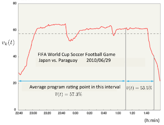
Figure 1: A typical behavior of program rating point. The data set is provided by Video Research Ltd. (http://www.videor.co.jp/eng/index.html)

As an example, in Fig. 1, we plot the empirical data for the rating point for the TV program of FIFA World Cup Soccer Football Game, Japan vs. Paraguay which was broadcasted in a Japanese television station on 29th June 2010. From this plot, we clearly observe two large valleys at 23:50 and 0:50. The first valley corresponds to the interval between the 1st half and the 2nd half of the game, whereas the second valley corresponds to the interval between 2nd half of the game and penalty shoot-out. In these intervals, a huge amount of viewers changed the channel to the other stations, and one can naturally assume that the program rating point remarkably dropped in these intervals. Hence, it might be possible to estimate the microscopic viewers’ decision makings from the macroscopic behavior of the time series such as the above program rating point.

Commercials usually being broadcasted on the television are now well-established as powerful and effective tools for sponsors to make viewers recognize their commodities or leading brand of the product or service. From the viewpoint of television stations, the commercial is quite important to make a profit as advertising revenue. However, at the same time, each television station has their own wishes to gather viewers of their program without any interruption due to the commercial because the commercial time is also a good chance for the viewers to change the channel to check the other programs which have been broadcasted from the other rival stations. On the other hand, the sponsors seek to maximize the so-called contact time with the viewers which has a meaning of duration of their watching the commercials for sponsors’ products or survives. To satisfy these two somehow distinct demands for the television station and sponsors, the best possible strategy is to lead the viewers not to zap to the other channels during their program. However, it is very hard requirement because we usually desire to check the other channels in the hope that we might encounter much more attractive programs in that time interval.

As the zapping action of viewers is strongly dependent on the preference of the viewers themselves in the first place, it seems to be very difficult problem for us to understand the phenomena by using exact scientific manner. However, if we consider the ‘ensemble’ of viewers to figure out the statistical properties of their collective behavior, the agent-based simulation might be an effective tool. Moreover, from the viewpoint of human engineering, there might exist some suitable channel locations for a specific television station in the sense that it is much easier for viewers to zap the channel to arrive as a man-machine interface.

With these mathematical and engineering motivations in mind, here we shall propose a simple mathematical model for zapping process of viewers. Our model system is numerically investigated by means of agent-based simulations. We evaluate several useful quantities such as television program rating point or gross rating point (GRP for short) from the microscopic description of the decision making by each viewer. Our approach enables us to investigate the television commercial market extensively like financial markets Ibuki .

This paper is organized as follows. In the next section 2, we introduce our mathematical model system and several relevant quantities such as the program rating point or the GRP. In section 3, we clearly introduce Ising spin-like variable which denotes the time-dependent microscopic state of a single viewer, a television station for a given arrangement of programs and commercials. In the next section 4, we show that the macroscopic quantities such as program rating point or the GRP are calculated in terms of the microscopic variables which is introduced in the previous section 3. In section 5, the energy function which specifies the decision making of each viewer is introduced explicitly. The energy function consists of three distinct parts, namely, a physical constraint on the controller, partial energies by exogenous and endogenous information. The exogenous part comes from advertisement of the program by the television station, whereas the endogenous part is regarded as the influence by the average program rating point on the past history of the market. By using the maximum entropy principle under several constraints, we derive the aggregation probability of viewers as a Gibbs-Boltzmann form. In section 6, we show our preliminary results obtained by computer simulations. We also consider the ‘adaptive location’ of commercial advertisements in section 7. In this section, we also consider the effects of the so-called Yamaba CMs, which are the successive CMs broadcasted intensively at the climax of the program, on the program rating points to the advertisement measurements. The last section is devoted to the concluding remarks.

2 The model system

We first introduce our model system of zapping process and submission procedure of each commercial into the public through the television programs. We will eventually find that these two probabilistic processes turn out to be our effective television commercial markets.

As long as we surveyed carefully, quite a lot of empirical studies on the effect of commercials on consumers’ interests have been done, however, up to now there are only a few theoretical studies concerning the present research topic to be addressed. For instance, Siddarth and Chattopadhyay Siddarth (see also the references therein) introduced a probabilistic model of zapping process, however, they mainly focused on the individual zapping action, and our concept of ‘collective behavior’ was not taken into account. Ohnishi et. al. Ikai tried to solve the optimal arrangement problem of television commercials for a given set of constraints in the literature of linear programming. Hence, it should be stressed that the goals of their papers are completely different from ours.

2.1 Agents and macroscopic quantities

To investigate the stochastic process of zapping process and its influence on the television commercial markets, we first introduce two distinct agents, namely, television stations, each of which is specified by the label $k=1,\cdots,K$ and viewers specified by the index $i=1,\cdots,N$. Here it should be noted that $K\ll N$ should hold. The relationship between these two distinct agents is described schematically in Fig.2.

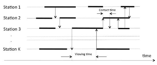
Figure 2: Two-types of agents in our model systems. The thick line segments denote the periods of commercial, whereas the thin line segments stand for the program intervals. The set of solid arrows describes a typical trajectory of viewer’s zapping processes. ‘Contact time’ and ‘viewing time’ are clearly defined as intervals for which the viewer watches the commercials and the programs, respectively. The duration and the procedures of casting television programs and CMs would be modeled by Poisson arrival processes. The detail accounts for them will be given in subsections 2.3, 2.4 and 2.5.

In this figure, the thick line segments denote the period of commercial, whereas the thin line segments stand for the program intervals. The set of solid arrows describes a typical trajectory of viewer’s zapping process. Then, the (instant) program rating point for the station $k$ at time $t$ is given by

$$v_{k}(t)=\frac{N_{k}(t)}{N}$$ (1)

where $N_{k}(t)$ is the number of viewers who actually watch the television program being broadcasted on the channel (the television station) $k$ at time $t$.

On the other hand, the time-slots for commercials are traded between the station and sponsors through the quantity, the so-called gross rating point (GRP) which is defined by

$$GRP^{(n)}_{k}=\frac{\theta_{k}^{(n)}}{T}\sum_{t=1}^{T}v_{k}(t)$$ (2)

where $T$ denotes total observation time, for instance, say $T=600$ minutes, for evaluating the program rating point. $\theta_{k}^{(n)}$ stands for the average contact time for viewers who are watching the commercial of the sponsor $n$ being broadcasted on the station $k$ during the interval $T$. Namely, the average GRP is defined by the product of the average program rating point and the average contact time. It should be noted that the equation (2) is defined as the average over the observation time $T$. Hence, if one seeks for the total GRP of the station $k$ over the observation time $T$, it should be given as $T\times GRP^{(n)}_{k}$. Therefore, the average GRP for the sponsor $n$ during the observation interval $T$ is apparently evaluated by the quantity: $GRP^{(n)}=(1/K)\sum_{k=1}^{K}GRP_{k}^{(n)}$ when one assumes that the sponsor $n$ asked all stations to broadcast their commercials through grand waves.

2.2 Zapping as a ‘stochastic process’

We next model the zapping process of viewers. One should keep in mind that here we consider the controller shown in Fig. 3.

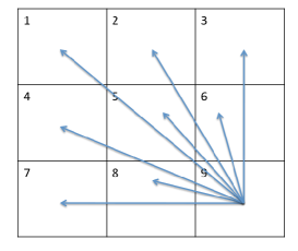
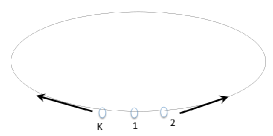
Figure 3: A typical television controller dealt with in this paper. The left panel shows ‘lattice-type’ channel, whereas the right is a typical channel of ‘ring-type’. Each channel location is modeled as shown in the corresponding cartoons in the lower two panels. Namely, the ‘lattice-type’ (left) and the ‘ring-type’ (right) for the modeling of the buttons on the television controller. Apparently, there exist a geometrical constraint on the latter type.

We should notice that (at least in Japan) there exist two types of channel locations on the controller, namely, ‘lattice-type’ and ‘ring-type’ as shown in Fig. 3. For the ‘lattice-type’, each button corresponding to each station is located on the vertex in the two-dimensional square lattice. Therefore, for the case of $K=9$ stations (channels) for example (See the lower left panel in Fig. 3), the viewers can change the channel from an arbitrary station $k$ to the other station $l(\neq k)$, and there is no geometrical constraint for users (viewers). Thus, we naturally define the transition probability $P(l|k)$ which is the probability that a user change the channel from station $k$ to $l(\neq k)$. Taking into account the normalization of the probabilities, we have $\sum_{l\neq k}^{K}P(l|k)=1,\,\,k=1,\cdots,K$. The simplest choice of the modeling of the transition probability satisfying the above constraint is apparently the uniform one and it is written by

$$P(l|k)=\frac{1}{K-1},\,\,\,k,l(\neq k)=1,\cdots,K.$$ (3)

On the other hand, for the ‘ring-type’ which is shown in the lower right panel of Fig. 3, we have a geometrical constraint $P(l=k\pm 1|k)>0,\,\,P(l\neq k\pm 1|k)=0$. From the normalization condition of the probabilities, we also have another type of constraint $P(l=k-1|k)+P(l=k+1|k)=1$ for $k,l(\neq k)=1,\cdots,K$. The simplest choice of the probability which satisfies the above constraints is given by $P(l=k-1|k)=P(l=k+1|k)=1/2$ for $k,l(\neq k)=1,\cdots,K$. Namely, the viewers can change from the current channel to the nearest neighboring two stations.

2.3 The duration of viewer’s stay

After changing the channel stochastically to the other rival stations, the viewer eventually stops to zap and stays the channel to watch the program if he or she is interested in it. Therefore, we should construct the probabilistic model of the length of viewer’s stay in both programs and commercials appropriately. In this paper, we assume that the lengths of the viewer $i$’s stay in the programs $\tau_{\rm on}$ (‘on’ is used as an abbreviation for ‘on air’) and commercials $\tau_{\rm cm}$ are given as ‘snapshots’ from the distributions:

$$P^{(i)}(\tau_{\rm on,cm})=a_{\tau_{\rm on,cm}}^{(i)}\,{\rm e}^{-\tau_{\rm on,cm}/a_{\tau_{\rm on,cm}}^{(i)}},\,\,\,i=1,\cdots,N$$ (4)

where $a_{\tau_{\rm on,cm}}^{(i)}$ stands for the ‘relaxation time’ of the viewer $i$ for the program and the commercial, respectively. Of course, $\tau_{\rm on,cm}$ fluctuates from person to person, hence, here we assume that $a_{\tau_{\rm on,cm}}^{(i)}$ might follow

$$a_{\tau_{\rm on,cm}}^{(i)}=c_{\rm on,cm}+\delta,\,\,P(\delta)=\mathcal{N}(0,\sigma^{2}).$$ (5)

Namely, the relaxation times for the program and commercial fluctuate around the typical value $c_{\rm on,cm}$ by a white Gaussian noise with mean zero and variance $\sigma^{2}$. Obviously, for ordinary viewers, $c_{\rm on}>c_{\rm cm}$ should be satisfied. We should notice that the above choice of the length of viewer’s stay is independent on the station, program or sponsor. For instance, the length of viewer’s stay in commercials might be changed according to the combination of commercials of different kinds of sponsors. However, if one needs, we can modify the model by taking into account the corresponding empirical data.

2.4 The process of casting commercials

Here we make a model of casting commercials by television stations. To make a simple model, we specify each sponsor by the label $n=1,\cdots,M$ and introduce microscopic variables $l_{k}(t)$ as follows.

$$l_{k}(t)=\left\{\begin{array}[]{ll}n\in\{1,\cdots,M\}&\mbox{(The station $k$ casts a CM of sponsor $n$ at time $t$)}\\ 0&\mbox{(The station $k$ casts a program at $t$)}\end{array}\right.$$ (6)

Hence, if one obtains $l_{1}(1)=l_{1}(2)=\cdots=l_{1}(10)=3$ and $l_{1}(11)=0$, then we conclude that the station $k=1$ casted the commercial of the sponsor $n=3$ from $t=1$ to $t=10$, and after this commercial period, the station $k$ resumed the program at the next step $t=11$. On the other hand, if we observe $l_{1}(1)=l_{1}(2)=\cdots=l_{1}(10)=3$ and $l_{1}(11)=2$, we easily recognize that the station $k=1$ casted the commercial of the sponsor $n=3$ from $t=1$ to $t=10$, and after this commercial period, the same station $k=1$ casted the commercial of the sponsor $n=2$ at the next step $t=11$. Therefore, for a given sequence of variables $l_{k}(t),\,k=1,\cdots,K$ for observation period $t=1,\cdots,T$, the possible patterns being broadcasted by all television stations are completely determined. Of course, we set $l_{k}(t),\,\,k=1,\cdots,K$ to the artificial values in our computer simulations, however, empirical evidence might help us to choose them.

2.5 Arrangement of programs and CMs

In following, we shall explain how each television station submits the commercials to appropriate time-slots of their broadcasting. First of all, we set $l_{k}(0)=0$ for all stations $k=1,\cdots,K$. Namely, we assume that all stations start their broadcasting from their own program instead of any commercials of their sponsors. Then, for an arbitrary $k$-th station, the duration $t_{\rm on}$ between the starting and the ending points of each section in the program is generated by the exponential distribution $\sim{\rm e}^{-t_{\rm on}/L_{\rm on}}$. Thus, from the definition, we should set $l_{k}(0)=\cdots=l_{k}({t_{\rm on}})=0$ for the resulting $t_{\rm on}$. We next choose a sponsor among the $M$-candidates by sampling from a uniform distribution in $[1,M]$. For the selected sponsor, say, $n\in\{1,M\}$, the duration of their commercial $t_{\rm cm}$ is determined by a snapshot of the exponential distribution $\sim{\rm e}^{-t_{\rm cm}/L_{\rm cm}}$. Thus, from the definition, we set $l_{k}(t_{\rm on}+1)=\cdots=l_{k}(t_{\rm on}+1+t_{\rm cm})=n$ for the given $t_{\rm cm}$ and $t_{\rm on}$. We repeat the above procedure from $t=0$ to $t=T-1$ for all stations $k=1,\cdots,K$. Apparently, we should choose these two relaxation times $L_{\rm on},L_{\rm cm}$ so as to satisfy $L_{\rm on}\gg L_{\rm cm}$. After this procedure, we obtain the realization of combinations of ‘thick’ (CMs) and ‘thin’ (television programs) lines as shown in Fig. 2.

3 Observation procedure

In the above section 2, we introduced the model system. To figure out the macroscopic behavior of the system, we should define the observation procedure. For this purpose, we first introduce microscopic binary (Ising spin-like) variables $S_{i,k}^{(l_{k}(t))}(t)\in\{0,1\}$ which is defined by

$$S_{i,k}^{(n)}(t)=\left\{\begin{array}[]{ll}1&\mbox{(The viewer $i$ watches the CM of sponsor $n$ on the station $k$ at time $t$)}\\ 0&\mbox{(The viewer $i$ does not watch the CM of $n$ on the station $k$ at time $t$)}\end{array}\right.$$ (7)

We should notice that for the case of $l_{k}(t)=0$, the Ising variable $S_{i,k}^{(l_{k}(t))}(t)$ takes

$$S_{i,k}^{(0)}(t)=\left\{\begin{array}[]{ll}1&\mbox{(The viewer $i$ watches the program on the station $k$ at time $t$)}\\ 0&\mbox{(The $i$ does not watch the program on the station $k$ at time $t$)}\end{array}\right.$$ (8)

Thus, the $K\times N$-matrix $\bm{S}^{(n)}(t)$ written by

$$\bm{S}^{(n)}(t)=\left(\begin{array}[]{ccc}S_{1,1}^{(n)}(t)&\cdots&S_{1,K}^{(n)}(t)\\ \cdots&\cdots&\cdots\\ \cdots&\cdots&\cdots\\ S_{N,1}^{(n)}(t)&\cdots&S_{N,K}^{(n)}(t)\end{array}\right)$$ (9)

becomes a sparsely coded large-size matrix which has only a single non-zero entry in each column. On the other hand, by summing up all elements in each row, the result, say $S_{1,k}^{(n)}+\cdots+S_{N,k}^{(n)}$ denotes the number of viewers who watch the commercial $n$ on the station $k$ at time $t$. Hence, if the number of sorts of commercials (sponsors) $M$ ($n\in\{1,\cdots,M\}$) is quite large, the element should satisfy $S_{1,k}^{(n)}+\cdots+S_{N,k}^{(n)}\ll N$ (Actually, it is a rare event that an extensive number of viewers watch the same commercial on the station $k$ at time $t$) and this means that the matrix $\bm{S}^{(n)}(t)$ is a sparse large-size matrix. It should be noted that macroscopic quantities such as program rating point or the GRP are constructed in terms of the Ising variables $S_{i,k}^{(l_{k}(t))}(t)\in\{0,1\}$.

For the Ising variables $S_{i,k}^{(l_{k}(t))}(t)\in\{0,1\}$, besides we already mentioned above, there might exist several constraints to be satisfied. To begin with, as the system has $N$-viewers, the condition $\sum_{l_{k}(t)=0}^{M}\sum_{k=1}^{K}\sum_{i=1}^{N}S_{i,k}^{(l_{k}(t))}(t)=N$ should be naturally satisfied. On the other hand, assuming that each viewer $i=1,\cdots,N$ watches the television without any interruption during the observation time $T$, we immediately have $\sum_{t=1}^{T}\sum_{l_{k}(t)=0}^{M}\sum_{k=1}^{K}S_{i,k}^{(l_{k}(t))}(t)=T,\,\,i=1,\cdots,N$. It should bear in mind that the viewer $i$ might watch the program or commercial brought by one of the $M$-sponsors, hence, we obtain the condition $\sum_{l_{k}(t)=0}^{M}\sum_{k=1}^{K}S_{i,k}^{(l_{k}(t))}(t)=1,\,\,i=1,\cdots,N,\,\,t=1,\cdots,T$.

These conditions might help us to check the validity of programming codes and numerical results.

4 Micro-descriptions of macro-quantities

In this section, we explain how one describes the relevant macroscopic quantities such as average program rating point or the GRP by means of a set of microscopic Ising variables $\{S_{i,k}^{(l_{k}(t))}(t)\}$ which was introduced in the previous section.

4.1 Instant and average program rating points

Here we should notice that the number of viewers who are watching the program or commercials being broadcasted on the station $k\,(=1,\cdots,K)$, namely, $N_{k}(t)$ is now easily rewritten in terms of the Ising variables at the microscopic level as $N_{k}(t)=\sum_{i=1}^{N}\sum_{l_{k}(t)=0}^{M}S_{i,k}^{(l_{k}(t))}(t)$. Hence, from equation (1), the instant program rating point of the station $k$ at time $t$, that is $v_{k}(t)$, is given explicitly as

$$v_{k}(t)=\frac{N_{k}(t)}{N}=\frac{1}{N}\sum_{i=1}^{N}\sum_{l_{k}(t)=0}^{M}S_{i,k}^{(l_{k}(t))}(t).$$ (10)

On the other hand, the average program rating point of the station $k$, namely, $\overline{v}_{k}$ is evaluated as $\overline{v}_{k}=(1/T)\sum_{t=1}^{T}v_{k}(t)$.

4.2 Contact time and cumulative GRP

We are confirmed that the contact time which was already introduced in the previous section 2 is now calculated in terms of $\{S_{i,k}^{(l_{k}(t))}(t)\}$ as follows. The contact time of the viewer $i$ with the commercial of the sponsor $n$ is written as

$$\theta_{i,k}^{(n)}=(1/T)\sum_{t=1}^{T}\sum_{l_{k}(t)=0}^{M}\delta_{l_{k}(t),n}S_{i,k}^{(l_{k}(t))}(t)$$ (11)

where $\delta_{a,b}$ denotes the Kronecker’s delta. It should be noted that we scaled the contact time over the observation time $T$ by $1/T$ so as to make the quantity the $T$-independent value. Hence, the average contact time of all viewers who watch the commercial of sponsor $n$ being broadcasted on the station $k$ is determined by $\theta_{k}^{(n)}\equiv(1/N)\sum_{i=1}^{N}\theta_{i,k}^{(n)}$. Thus, the cumulative GRP is obtained from the definition (2) as

$$GRP_{k}^{(n)} = \frac{1}{T}\sum_{t=1}^{T}v_{k}(t)\times\theta_{k}^{(n)}$$ (12)

$$= \frac{1}{N^{2}T^{2}}\left(\sum_{t=1}^{T}\sum_{i=1}^{N}\sum_{l_{k}(t)=0}^{M}S_{i,k}^{(l_{k}(t))}(t)\right)\left(\sum_{i=1}^{N}\sum_{t=1}^{T}\sum_{l_{k}(t)=0}^{M}\delta_{l_{k}(t),n}S_{i,k}^{(l_{k}(t))}(t)\right).$$

From the above our argument, we are now confirmed that all relevant quantities in our model system could be calculated in terms of the Ising variables $\{S_{i,k}^{(l_{k}(t))}(t)\}$ which describe the microscopic state of ingredients in the commercial market.

However, the matrix $\bm{S}^{(n)}(t)$ itself is determined by the actual stochastic processes of viewer’s zapping with arranging the programs and television commercials. Therefore, in the next section, we introduce the energy(cost)-based zapping probability which contains the random selection (3) as a special case for the ‘lattice-type’ controller.

5 Energy function of zapping process

As we showed in the literature of our probabilistic labor market Chen , it is convenient for us to construct the energy function to quantify the action of each viewer. The main issue to be clarify in this study is the condition on which concentration (‘condensation’) of viewers to a single television station is occurred due to the endogenous information. The same phenomena refereed to as informational cascade in the financial market is observed by modeling of the price return by means of magnetization in the Ising model Ibuki2 . In the financial problem, the interaction $J_{ij}$ between Ising spins $S_{i}$ and $S_{j}$ corresponds to endogenous information, whereas the external magnetic field $h_{i}$ affected on the spin $S_{i}$ stands for the exogenous information. However, in our commercial market, these two kinds of information would be described by means of a bit different manner. It would be given below.

5.1 Physical constraints on television controllers

For this end, let us describe here the location of channel for the station $k$ on the controller as a vertex on the two-dimensional square lattice (grid) as $\bm{Z}_{k}\equiv(x_{k},y_{k})$. Then, we assume that the channel located on the vertex at which the distance from the channel $k$ is minimized might be more likely to be selected by the viewer who watches the program (or commercial) on the station $k$ at the instance $t$. In other words, the viewer minimizes the energy function given by $\gamma(\bm{Z}_{k}-\bm{Z}_{l})^{2}\,\,\,(l\neq k)$, where we defined the $L_{2}$-norm as the distance $(\bm{Z}_{k}-\bm{Z}_{l})^{2}\equiv(x_{k}-x_{l})^{2}+(y_{k}-y_{l})^{2}$. The justification of the above assumption should be examined from the viewpoint of human-interface engineering.

5.2 Exogenous information

Making the decision of viewers is affected by the exogenous information. For instance, several weeks before World Cup qualifying game, a specific station $\overline{k}$, which will be permitted to broadcast the game, might start to advertise the program of the match. Then, a large fraction of viewers including a soccer football fan might decide to watch the program at the time. Hence, the effect might be taken into account by introducing the energy $-\zeta\prod_{\xi=s}^{e}\delta_{t_{\xi},t}\delta_{l,\overline{k}}$ where $t_{s}$ denotes the time at which the program starts and $t_{e}$ stands for the time of the end. Therefore, the energy decreases when the viewer watches the match of World Cup qualifying during the time for the program, namely from $t=t_{s}$ to $t_{e}$ ($\Delta t\equiv t_{e}-t_{s}$: broadcasting hours of the program).

5.3 Endogenous information

The collective behavior might be caused by exogenous information which is corresponding to ‘external field’ in the literature of statistical physics. However, collective behavior of viewers also could be ‘self-organized’ by means of endogenous information. To realize the self-organization, we might use the moving average of the instant program rating over the past $L$-steps ($L\ll T$), namely,

$$\langle v_{k}(t)\rangle\equiv\frac{1}{L}\sum_{\rho=t-L}^{t-1}v_{k}(\rho)$$ (13)

as the endogenous information. Then, we define the ‘winner channel’ which is more likely to be selected at time $t$ as $\hat{k}=\arg\max_{m}\langle v_{m}(t)\rangle$ (One might extend it to a much more general form:

$$\hat{k}=\arg\max_{m}\langle v_{m}(r)\rangle$$ (14)

for a given ‘time lag’ $r\,(<t)$). Henceforth, we assume that if the winner channel $\hat{k}$ is selected, a part of total energy $-\beta\delta_{l,\hat{k}}$ decreases. This factor might cause the collective behavior of $N$-individual viewers. Of course, if one needs, it might be possible for us to recast the representation of the winner channel $\hat{k}$ by means of microscopic Ising variables $\{S_{i,k}^{(l_{k}(t)}(t)\}$.

Usually, the collective behavior is caused by direct interactions (connections) between agents. However, nowadays, watching television is completely a ‘personal action’ which is dependent on the personal preference because every person can possess their own television due to the wide-spread drop in the price of the television set. This means that there is no direct interaction between viewers, and the collective behavior we expect here might be caused by some sorts of public information such as program rating point in the previous weeks. In this sense, we are confirmed that the above choice of energy should be naturally accepted.

Therefore, the total energy function at time $t$ is defined by

$$E_{k}(l)\equiv\gamma(\bm{Z}_{k}-\bm{Z}_{l})^{2}-\zeta\prod_{\xi=s}^{e}\delta_{t_{\xi},t}\delta_{l,\overline{k}}-\beta\delta_{l,\hat{k}}$$ (15)

with $\hat{k}=\arg\max_{m}\langle v_{m}(t)\rangle$, where $\beta,\zeta,\gamma\geq 0$ are model parameters to be estimated from the empirical data in order to calibrate our model system. According to the probabilistic labor market which was introduced by one of the present authors, we construct the transition probability $P(l|k)$ as the Gibbs-Boltzmann form by solving the optimization problem of the functional:

$$f[P(l|k)]\equiv-\sum_{l\neq k}P(l|k)\log P(l|k)-\lambda\left\{\sum_{l\neq k}P(l|k)-1\right\}-\lambda^{{}^{\prime}}\left\{\sum_{l\neq k}E_{k}(l)P(l|k)-E\right\}$$ (16)

with respect to $P(l|k)$. Then, we immediately obtain the solution of the optimization problem (variational problem) as

$$P(l|k) = \frac{{\exp}[-E_{k}(l)]}{\sum_{l\neq k}{\exp}[-E_{k}(l)]}$$

$$= \frac{{\exp}[-\gamma(\bm{Z}_{k}-\bm{Z}_{l})^{2}+\zeta\prod_{\xi=s}^{e}\delta_{t_{\xi},t}\delta_{l,\overline{k}}+\beta\delta_{l,\hat{k}}]}{\sum_{l\neq k}{\exp}[-\gamma(\bm{Z}_{k}-\bm{Z}_{l})^{2}+\zeta\prod_{\xi=s}^{e}\delta_{t_{\xi},t}\delta_{l,\overline{k}}+\beta\delta_{l,\hat{k}}]}$$

where we chose one of the Lagrange multipliers in $f[P(l|k)]$ as $\lambda=\log\{\sum_{l\neq k}P(l|k)\}-1$, and another one $-\lambda^{{}^{\prime}}$ is set to $1$ for simplicity, which has a physical meaning of ‘unit inverse-temperature’. We should notice that in the ‘high-temperature limit’ $\beta,\zeta,\gamma\to 0$, the above probability becomes identical to that of the random selection (3). These system parameters should be calibrated by the empirical evidence.

In the above argument, we focused on the ‘lattice-type’ controller, however, it is easy for us to modify the energy function to realize the ‘ring-type’ by replacing $\gamma(\bm{Z}_{k}-\bm{Z}_{l})^{2}$ in (15) by $\varepsilon_{l}\equiv-\gamma(\delta_{l,k+1}+\delta_{l,k-1})$, namely, the energy decreases if and only if the viewer who is watching the channel $k$ moves to the television station $k-1$ or $k+1$. This modification immediately leads to

$$P(l|k)=\frac{{\exp}[-E_{k}(l)]}{\sum_{l\neq k}{\exp}[-E_{k}(l)]}=\frac{{\exp}[-\varepsilon_{l}+\zeta\prod_{\xi=s}^{e}\delta_{t_{\xi},t}\delta_{l,\overline{k}}+\beta\delta_{l,\hat{k}}]}{\sum_{l\neq k}{\exp}[-\varepsilon_{l}+\zeta\prod_{\xi=s}^{e}\delta_{t_{\xi},t}\delta_{l,\overline{k}}+\beta\delta_{l,\hat{k}}]}.$$ (17)

We are easily confirmed that the transition probability for random selection in the ‘ring-type’ controller is recovered by setting $\zeta=\beta=0$ as

$$P(k-1|k)=\frac{{\rm e}^{\gamma}}{{\rm e}^{\gamma}+{\rm e}^{\gamma}}=\frac{1}{2}=P(k+1|k)$$

and $P(l|k)=0$ for $l\neq k\pm 1$.

In the next section, we show the results from our limited contributions by computer simulations.

6 A preliminary: computer simulations

In this section, we show our preliminary results. In Fig. 4, we plot the typical behavior of instant program rating point $v_{k}(t)$ for $k=1,\cdots,K$. We set $K=9,N=600,M=1$ and $T=600$ for the case of the simplest choice $\beta=\zeta=\gamma=0$ leading up to (3) (‘high-temperature limit’). This case might correspond to the ‘unconscious zapping’ by viewers. The parameters appearing in the system are chosen as $L_{\rm on}=c_{\rm on}=12$ and $L_{\rm cm}=c_{\rm cm}=4$. The upper panel shows the result of ‘lattice-type’ channel location on the controller, whereas the lower panel is the result of ‘ring-type’.

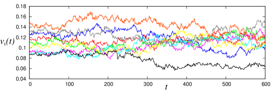
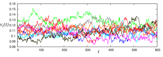
Figure 4: Typical behavior of instant program rating point $v_{k}(t)$ for $k=1,\cdots,K$. Here we set $K=9,M=1,N=600$ and $T=600$. The parameters appearing in the system are chosen as $L_{\rm on}=c_{\rm on}=12$ and $L_{\rm cm}=c_{\rm cm}=4$. The upper panel is the result of ‘lattice-type’ with $\beta=\zeta=\gamma=0$, whereas the lower panel shows the case of ‘ring-type’. We clearly find that the result of ring-type is less volatile than that of the lattice-type.

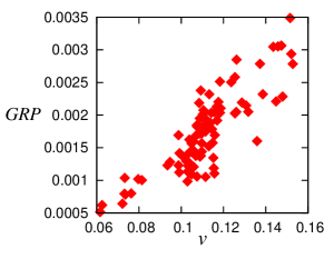
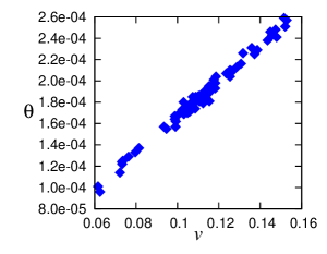
Figure 5: The two-dimensional scattered plot for the average program rating point: $v\equiv(1/K)\sum_{k=1}^{K}\overline{v}_{k}$ and the average cumulative GRP: $GRP\equiv(1/K)\sum_{k=1}^{K}GRP_{k}^{(1)}$ for the case of ‘lattice-type’ channel location (left). The right panel shows the scatter plot with respect to the $v$ and the effective contact time which is defined by $\theta\equiv(1/KT)\sum_{k=1}^{K}\theta_{k}^{(1)}$ (We have only a single sponsor). The parameters are set to the same values as in Fig. 4.

In Fig. 5 (left), we display the scattered plot with respect to the GRP and the average program rating point for the case of ‘lattice-type’ channel location. From this figure, we find that there exists a remarkable positive correlation between these two quantities (the Pearson coefficient is $0.85$). This fact is a justification for us to choose the GRP as a ‘market price’ for transactions. In the right panel of this figure, the scattered plot with respect to the GRP and the effective contact time defined by $(1/KT)\sum_{k=1}^{K}\theta_{k}^{(1)}$ is shown. It is clearly found that there also exists a positive correlation with the Pearson coefficient $0.9914$.

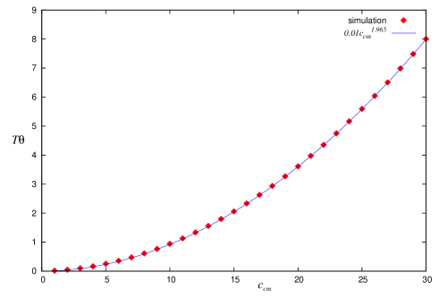
Figure 6: The $c_{\rm cm}$-dependence of the $T$-scaled effective contact time $T\theta$. We set the observation time $T=60$ and the other parameters are set to the same values as in Fig. 4. We also plot the well-fitting curve $0.01c_{\rm cm}^{1.965}$ for eyes’ guide.

We also plot the $c_{\rm cm}$-dependence of the $T$-scaled effective contact time $T\theta$ in Fig. 6. This figure tells us that the frequent zapping actions reduce the contact time considerably and it becomes really painful for the sponsors.

6.1 Symmetry breaking due to endogenous information

We next consider the case in which each viewer makes his/her decision according to the market history, namely, we choose $\gamma=1,\zeta=0$ and set the value of $\beta$ to $\beta=0$ and $\beta=1.8$. We show the numerical results in Fig. 7.

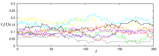
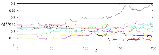
Figure 7: Typical behavior of instant program rating point $v_{k}(t)$ for $k=1,\cdots,K$. Here we set $K=9,M=1,N=600$ and $T=200$. The parameters which specify the energy function of ‘lattice-type’ controller are chosen as $(\gamma,\zeta,\beta)=(1,0,0)$ (the upper panel) and $(\gamma,\zeta,\beta)=(1,0,1.8)$ (the lower panel) with the history length $L=5$. The parameters appearing in the system are chosen as the same values as in Fig. 4.

From this panels, we find that the instant program rating point $v_{k}(t)$ for a specific television station increases so as to become a ‘monopolistic station’ when each viewer starts to select the station according to the market history, namely, $\beta>0$. In other words, the symmetry of the system with respect to the program rating point is broken as the parameter $\beta$ increases.

To measure the degree of the ‘symmetry breaking’ in the behavior of the instant program rating points more explicitly, we introduce the following order parameter:

$$B(t)\equiv\frac{1}{K}\sum_{k=1}^{K}\left|v_{k}(t)-\frac{1}{K}\right|$$ (18)

which is defined as the cumulative difference between $v_{k}$ and the value for the ‘perfect equality’ $1/K$. We plot the $B(t)$ for the case of $\beta=0,1$ and $2$. For finite $\beta$, the symmetry is apparently broken around $t=100$ and the system changes from symmetric phase (small $B(t)$) to the symmetry breaking phase (large $B(t)$).

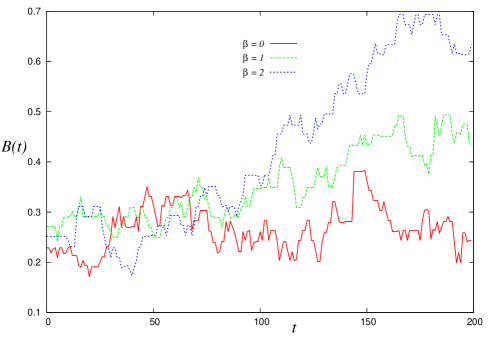
Figure 8: The behavior of order parameter $B(t)$ which measures the degree of symmetry breaking in the $v_{k}$. The symmetry is apparently broken for $\beta=1,2$ around $t=100$ and the system changes from symmetric phase (small $B(t)$) to the symmetry breaking phase (large $B(t)$).

We next evaluate the degree of the symmetry breaking by means of the following Shannon’s entropy:

$$H(t)=-\sum_{k=1}^{K}v_{k}(t)\log v_{k}(t)$$ (19)

where the above $H(t)$ takes the maximum for the symmetric solution $v_{k}(t)=1/K$ as

$$H(t)=-K\times\frac{1}{K}\log(1/K)=\log K$$ (20)

whereas the minimum $H(t)=0$ is achieved for $v_{k}=1$ and $v_{k^{{}^{\prime}}\neq k}=0$, which is apparently corresponding to the symmetry breaking phase. In Fig. 9, we plot the $H(t)$ for several choices of $\beta$ as $\beta=0,1$ and $2$. From this figure, we find that for finite $\beta$, the system gradually moves from the symmetric phase to the symmetry breaking phase due to the endogenous information (e.g. word-of-mouth communication).

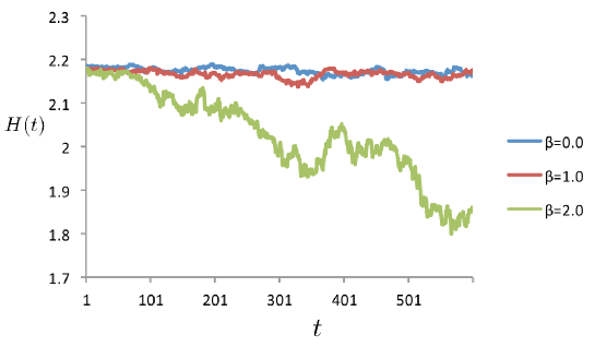
Figure 9: A typical behavior of the Shannon’s entropy $H(t)$.

Finally, we consider the the time lag $r$-dependence (see equation (14)) of the resulting $v_{k}(t)$. The result is shown in Fig. 10.

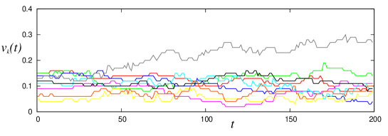
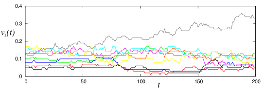
Figure 10: Typical behavior of instant program rating point $v_{k}(t)$ for $k=1,\cdots,K$ for the choice of the time lag $r=10$ (the upper panel) and $r=40$ (the lower panel). Here we set $K=9,M=1,N=600$ and $T=200$. The parameters which specify the energy function of ‘lattice-type’ controller are chosen as $(\gamma,\zeta,\beta)=(1,0,1.5)$ with history length $L=5$. The parameters appearing in the system are chosen as the same values as in Fig. 4.

From this figure, we clearly find that the large time lag $r$ causes the large amount of symmetry breaking in the program rating point $v_{k}(t)$.

7 Adaptive location of commercials

In the subsection 2.4, we assumed that each commercial advertisement is posted according to the Poisson process. However, it is rather artificial and we should consider the case in which each television station decides the location of the commercials using the adaptive manner. To treat such case mathematically, we simply set $K=2$ and $M=1$, namely, only two stations cast the same commercial of a single sponsor. Thus, we should notice that one can define $l_{k}(t)=0$ (on air) or $l_{k}(t)=1$ (CM) for $k=0,1$.

Then, we assume that each television station decides the label $l_{k}(t)$ according to the following successive update rule of the CM location probability:

$$P(l_{k}(t)) = \frac{1}{4}\left\{1+(2l_{k}(t)-1)\tanh\Omega\left(L_{c}-\sum_{\rho=t-1}^{t-\mathcal{L}}l_{k}(\rho)\right)\right\}$$ (21)

$$\times \left\{1+(2l_{k}(t)-1)\tanh\Omega\left(\frac{v_{0}(t-\tau)-v_{0}(t-1)}{\tau}\right)\right\}$$

for $k=0,1$, which means that if the cumulative commercial time by the duration $\mathcal{L}$, that is, $\sum_{\rho=t-1}^{t-\mathcal{L}}l_{k}(\rho)$ is lower than $L_{c}$, or if the slope of the program rating point $v_{k}$ during the interval $\tau$ is negative, the station $k$ is more likely to submit the commercial at time $t$.

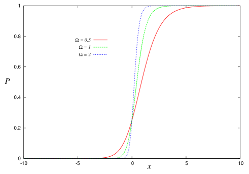
Figure 11: The behavior of $P(x)=(1+\tanh(\Omega x))(1+\tanh(\Omega x))/4$.

It should be noted that in the limit of $\Omega\to\infty$, the above probabilistic location becomes the following deterministic location model (see also Fig. 11)

$$l_{k}(t)=\Theta\left(L_{c}-\sum_{\rho=t-1}^{t-\mathcal{L}}l_{k}(\rho)\right)\Theta\left(\frac{v_{k}(t-\tau)-v_{k}(t-1)}{\tau}\right)$$ (22)

for $k=0,1$. From the nature of two television stations, $v_{0}(t-1)+v_{1}(t-1)=1$ and $v_{0}(t-\tau)+v_{1}(t-\tau)=1$ should be satisfied. Thus, the possible combinations of $(l_{0}(t),l_{1}(t))$ are now restricted to $(l_{0}(t),l_{1}(t))=(0,0),(0,1),(1,0)$, and $(l_{0}(t),l_{1}(t))=(1,1)$ is not allowed to be realized. In other words, for the deterministic location model described by (22), there is no chance for the stations $k=0,1$ to cast the same CM advertisement at the same time.

On the other hand, the viewer also might select the station according to the length of the commercial times in the past history. Taking into account the assumption, we define the station $\tilde{k}$ by

$$\tilde{k}=\frac{1}{2}\left\{1-{\rm sgn}(\langle l_{1}(t)\rangle-\langle l_{0}(t)\rangle)\right\}$$ (23)

with

$$\langle l_{k}(t)\rangle\equiv(1/\mathcal{L})\sum_{\rho=t-1}^{t-\mathcal{L}}l_{k}(t),\,\,\,k=0,1.$$ (24)

Then, the $\tilde{k}$ denotes the station which casted shorter commercial times during the past time steps $\mathcal{L}$ than the other. Hence, we rewrite the energy function for the two stations model in terms of the $\tilde{k}$ as follows.

$$E_{k}(l)\equiv-\zeta\prod_{\xi=s}^{e}\delta_{t_{\xi},t}\delta_{l,\overline{k}}-\beta\delta_{l,\hat{k}}-\xi\delta_{l,\tilde{k}}$$ (25)

where we omitted the term $\gamma(\bm{Z}_{k}-\bm{Z}_{l})^{2}$ due to the symmetry $(\bm{Z}_{0}-\bm{Z}_{1})^{2}=(\bm{Z}_{1}-\bm{Z}_{0})^{2}$. As the result, the transition probability is rewritten as follows.

$$P(l|k)=\frac{{\exp}[\zeta\prod_{\xi=s}^{e}\delta_{t_{\xi},t}\delta_{l,\overline{k}}+\beta\delta_{l,\hat{k}}+\xi\delta_{l,\tilde{k}}]}{\sum_{l\neq k}{\exp}[\zeta\prod_{\xi=s}^{e}\delta_{t_{\xi},t}\delta_{l,\overline{k}}+\beta\delta_{l,\hat{k}}+\xi\delta_{l,\tilde{k}}]}$$ (26)

The case without the exogenous information, that is, $\zeta=0$, we have the following simple transition probability for two stations.

$$P(1|0)=\frac{{\exp}(\beta\delta_{1,\hat{k}}+\xi\delta_{1,\tilde{k}})}{{\exp}(\beta\delta_{0,\hat{k}}+\xi\delta_{0,\tilde{k}})+{\exp}(\beta\delta_{1,\hat{k}}+\xi\delta_{1,\tilde{k}})}$$ (27)

$$P(0|1)=\frac{{\exp}(\beta\delta_{0,\hat{k}}+\xi\delta_{0,\tilde{k}})}{{\exp}(\beta\delta_{0,\hat{k}}+\xi\delta_{0,\tilde{k}})+{\exp}(\beta\delta_{1,\hat{k}}+\xi\delta_{1,\tilde{k}})}$$ (28)

with $P(0|0)=1-P(1|0)$ and $P(1|1)=1-P(0|1)$.

We simulate the CM advertisement market described by (27)(28) and (22) and show the limited result in Fig. 12.

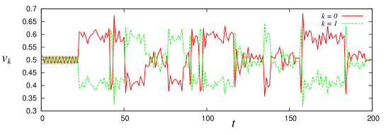
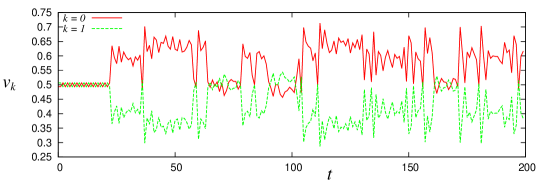
Figure 12: Typical behavior of instant program rating points $v_{k}(t)$ for the two stations $k=0,1$ which are generated by the adaptive CM locations (22) and zapping probabilities (28)(27). We chose $\beta=0$ (the upper panel) and $\beta=1$ (the lower panel). Here we set $M=1,N=600$ and $T=200$. The parameters which specify the energy function and CM locations are chosen as $\zeta=1,L_{c}=2,L=\mathcal{L}=\tau=20(=T/10)$. The other parameters appearing in the system are chosen as the same values as in Fig. 4.

From this figure, we find that for the case of $\beta=0$, the superiority of two stations changes frequently, however, the superiority is almost ‘frozen’, namely, the superiority does not change in time when we add the endogenous information to the system by setting $\beta=1$. For both cases ($\beta=0,1$), the behavior of the instant program rating as a ‘macroscopic quantity’ seems to be ‘chaotic’. The detail analysis of this issue should be addressed as one of our future studies.

7.1 Frequent CM locations at the climax of program

The results given in the previous sections partially have been reported by the present authors in the reference Kyan . Here we consider a slightly different aspect of the television commercial markets.

Recently in Japan, we sometimes have encountered the situation in which a television station broadcasts their CMs frequently at the climax of the program. Especially, in a quiz program, a question master speaks with an air of importance to open the answer and the successive CMs start before the answer comes out. Even after the program restarts, the master puts on airs and he never gives the answer and the program is again interrupted by the CMs. This kind of CMs is now refereed to as Yamaba CM (‘Yamaba’ has a meaning of ‘climax’ in Japanese). To investigate the psychological effects on viewers’ mind, Sakaki Sakaki carried out a questionnaire survey and the result is given in Table 1.

Question	Yes	I do not know	No
Is Yamaba CM unpleasant?	86 $\%$	7 $\%$	7 $\%$
Is Yamaba CM not favorable?	84 $\%$	14 $\%$	2 $\%$
Do you purchase the product advertised by Yamaba CM?	66 $\%$	37 $\%$	97 $\%$

Table 1: A questionnaire survey for viewers’ impression on the so-called Yamaba CM Sakaki .

From this table, we find that more than eighty percent of viewers might feel that the Yamaba CM is unpleasant and not favorable. With this empirical fact in mind, in following, we shall carry out computer simulations in which the CMs broadcasted by a specific television station are located intensively at the climax of the program.

Effects on the program rating points

We first consider the effects of the Yamaba CMs on the program rating points. The results are shown in Fig. 13 as a typical behavior of the program rating points $v_{k}(t),\,k=1,\cdots,9$. In this simulation, we fix the total length of CMs in a program so as to be less than eighteen percent of the total broadcasting time $T$ of the whole program including CMs. In the upper panel, we distribute the CMs of all television stations randomly, whereas in the lower panel, the CMs of a specific station (the line in the panel is distinguished from the other eight stations by a purple thick line) are located intensively at the climax (the end of the program) and for the other eight stations, the CMs are located randomly. The other conditions in the simulations are selected as the same as in Fig. 4.

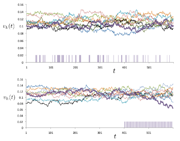
Figure 13: The resulting program rating points for random locations of CMs (the upper panel) and for biased locations of CMs for a specific television station (say, $k=1$, the line in the panel is distinguished from the other eight stations by a purple thick line). The perpendicular purple lines stand for the period of CMs for the specific station $k=1$.

From this figure, we find that the program rating point for the station $k=1$ which broadcasts Yamaba CMs intensively at the climax apparently decreases at the climax in comparison with the other stations.

To check the effect of the relaxation time $L_{\rm cm}$ on the results, we carry out the simulation by changing the value as $L_{\rm cm}=1,2,3$ and $5$. The results are shown in Fig. 14.

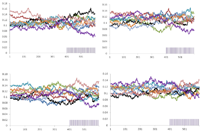
Figure 14: The $L_{\rm cm}$-dependence of the program rating points $v_{k}(t),\,k=1,\cdots,9$ shown in Fig. 13. From the upper left to the lower right, $L_{\rm cm}=1,2,3$ and $L_{\rm cm}=5$.

From this figure, we clearly find that the program rating point for the station $k=1$ which broadcasts Yamaba CMs intensively at the climax apparently decreases around $t=t_{\rm c}=400$ and the $t_{\rm c}$ is independent of the length of $L_{\rm cm}$.

Effects on the advertisement measurements

We next evaluate of the effects of the so-called Yamaba CMs on the advertisement measurements such as the GRP or average contact time of the CMs by viewers. To quantify the effects, we consider the $GRP_{k}$-$\overline{v}_{k}$ diagram for $K=9$ stations, where $GRP_{k}\equiv GRP_{k}^{(1)}$ in the definition of (12) because now we consider the case of $M=1$ for simplicity. We plot the result in Fig. 15 (left). In this panel, there is no station broadcasting the Yamaba CMs. When we define the advertisement efficiency $\eta$ for the sponsor by the slope of these points, the efficiency for this unbiased case is $\eta\simeq 0.9748$. We next consider the case in which a specific station, say, $k=1$ broadcasts the Yamaba CMs. The results are shown in the right panel of Fig. 15.

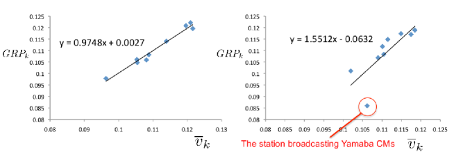
Figure 15: The $GRP_{k}$-$\overline{v}_{k}$ diagram for $K=9$ stations. Each point corresponds to each station. In the left panel, there is no station broadcasting the so-called Yamaba CMs, whereas only a specific station, say $k=1$ is broadcasting the Yamaba CMs in the right panel. We set $M=1,N=T=600$.

From this panel, we are confirmed that the both $GRP_{k=1}$ and $\overline{v}_{k=1}$ apparently decrease in comparison with the other eight stations. Hence, the slope $\eta$ calculated by the eight stations (except for $k=1$) increases up to $\eta\simeq 1.5512$ because viewers who was watching the program of the station $k=1$ moved (changed the channel) to the other eight stations and it might increase the $GRP_{k\neq 1}$ and $\overline{v}_{k\neq 1}$ extensively.

From the results given in this section, we might conclude that the Yamaba CMs (biased CM locations) are not effective from the view points of viewers, sponsors and television stations although our simulations were carried out for limited artificial situations.

8 Concluding remarks

We proposed a ‘theoretical platform’ to investigate the human collective behavior in the macroscopic scale through viewers’ zapping actions at the microscopic level. We just showed a very preliminary result without any comparison with empirical data. However, several issues, in particular, much more mathematically rigorous argument based on the queueing theory Inoue , data visualization via the MDS Ibuki3 , portfolio optimization Livan and a mathematical relationship between our system and the so-called regime-switching processes Yin should be addressed as our future studies.

Acknowledgements

This work was financially supported by Grant-in-Aid for Scientific Research (C) of Japan Society for the Promotion of Science, No. 22500195. One of the present authors (JI) thanks Nivedita Deo, Sanjay Jain, Sudhir Shah for fruitful discussion at the workshop: Exploring an Interface Between Economics $\&$ Physics at University of Delhi. He also thanks George Yin at Department of Mathematics, Wayne State University, USA, for drawing our attention to the reference Yin . We thank organizers of Econophysics-Kolkata VII, in particular, Frederic Abergel, Anirban Chakraborti, Asim K. Ghosh, Bikas K. Chakrabarti and Hideaki Aoyama.

References

- (1) C.W. Reynolds, Flocks, Herds, and Schools: A Distributed Behavioral Model, Computer Graphics 21, 25 (1987).
- (2) M. Makiguchi and J. Inoue, Numerical Study on the Emergence of Anisotropy in Artificial Flocks: A BOIDS Modelling and Simulations of Empirical Findings, Proceedings of the Operational Research Society Simulation Workshop 2010 (SW10), CD-ROM, pp. 96-102 (the preprint version, arxiv:1004 3837) (2010). See also M. Makiguchi and J. Inoue, Emergence of Anisotropy in Flock Simulations and Its Computational Analysis, Transactions of the Society of Instrument and Control Engineers 46, No. 11, pp. 666-675 (2010) (in Japanese).
- (3) T. Ibuki and J. Inoue, Response of double-auction markets to instantaneous Selling-Buying signals with stochastic Bid-Ask spread, Journal of Economic Interaction and Coordination 6, No.2, pp. 93-120 (2011).
- (4) S. Siddarth and A. Chattopadhyay, To Zap or Not to Zap: A Mixture Model of Channel Switching During Commercials, Working Paper, Series No. MKTG97.091 (1997).
- (5) H. Ohnishi, K. Ishida, H. Aoyama, Y. Saruwatari and M. Ikai, The Operations Research Society of Japan 50, No. 3, pp. 151-158 (2005) (in Japanese).
- (6) H. Chen and J. Inoue, Dynamics of probabilistic labor markets: statistical physics perspective, Lecture Notes in Economics and Mathematical Systems 662, pp. 53-64, “Managing Market Complexity”, Springer (2012), H. Chen and J. Inoue, Statistical Mechanics of Labor Markets, Econophysics of systemic risk and network dynamics, New Economic Windows, Springer-Verlag (Italy-Milan), pp. 157-171 (2013).
- (7) T. Ibuki, S. Higano, S. Suzuki and J. Inoue, Hierarchical information cascade: visualization and prediction of human collective behaviour at financial crisis by using stock-correlation, ASE Human Journal 1, Issue 2, pp. 74-87 (2012).
- (8) H. Kyan and J. Inoue, Modeling television commercial advertisement markets: To zap or not to zap, that is the question for sponsors of TV programs, Proceedings of IEEE/SICE Symposium SII2012, CD-ROM, pp. 816-823 (2012).
- (9) H. Sakaki, Annual Report of Nikkei Advertising Research Institute 255, pp. 19-26 (2011).
- (10) N. Sazuka, J. Inoue and E. Scalas, The distribution of first-passage times and durations in FOREX and future markets, Physica A 388, No. 14, pp. 2839-2853 (2009), J. Inoue and N. Sazuka, Queueing theoretical analysis of foreign currency exchange rates, Quantitative Finance 10, No. 10, pp. 121-130 (2010).
- (11) T. Ibuki, S. Suzuki and J. Inoue, Cluster Analysis and Gaussian Mixture Estimation of Correlated Time-Series by Means of Multi-dimensional Scaling, Econophysics of systemic risk and network dynamics, New Economic Windows, Springer-Verlag (Italy-Milan), pp. 239-259 (2013).
- (12) G. Livan, J. Inoue and E. Scalas, On the non-stationarity of financial time series: impact on optimal portfolio selection, Journal of Statistical Mechanics, P07025 (2012).
- (13) S.L. Nguyen and G. Yin, Weak convergence of Markov-modulated random sequences, Stochastics: An International Journal of Probability and Stochastic Processes 82, No. 6, pp. 521-552 (2010).