Fluid preconditioning for Newton-Krylov-based, fully implicit, electrostatic particle-in-cell simulations

Abstract

A recent proof-of-principle study proposes an energy- and charge-conserving, nonlinearly implicit electrostatic particle-in-cell (PIC) algorithm in one dimension [Chen et al, J. Comput. Phys., 230 (2011) 7018]. The algorithm in the reference employs an unpreconditioned Jacobian-free Newton-Krylov method, which ensures nonlinear convergence at every timestep (resolving the dynamical timescale of interest). Kinetic enslavement, which is one key component of the algorithm, not only enables fully implicit PIC a practical approach, but also allows preconditioning the kinetic solver with a fluid approximation. This study proposes such a preconditioner, in which the linearized moment equations are closed with moments computed from particles. Effective acceleration of the linear GMRES solve is demonstrated, on both uniform and non-uniform meshes. The algorithm performance is largely insensitive to the electron-ion mass ratio. Numerical experiments are performed on a 1D multi-scale ion acoustic wave test problem.

1 Introduction

The Particle-in-cell (PIC) method solves Vlasov-Maxwell’s equations for kinetic plasma simulations [1, 2]. In the standard approach, Maxwell’s equations (or in the electrostatic limit, Poisson equation) are solved on a grid, and the Vlasov equation is solved by method of characteristics using a large number of particles, from which the evolution of the probability distribution function (PDF) is obtained. The field-PDF description is tightly coupled. Maxwell’s equations (or a subset thereof) are driven by moments of the PDF such as charge density and/or current density. The PDF, on the other hand, follows a hyperbolic equation in phase space, whose characteristics are self-consistently determined by the fields.

To date, most PIC methods employ explicit time-stepping (e.g. leapfrog scheme), which can be very inefficient for long-time, large spatial scale simulations. The algorithmic inefficiency of standard explicit PIC is rooted in the presence of numerical stability constraints, which force both a minimum grid-size (due to the so-called finite-grid instability [1, 2], which requires resolution of the smallest Debye length) and a very small timestep (due to the well-known CFL constraint, which requires resolution of the fastest plasma wave, or in the more general electromagnetic case, the light wave). Moreover, a fundamental issue with explicit schemes is numerical heating due to the lack of exact energy conservation in a discrete setting [1, 2], which makes the accuracy of explicit PIC simulations questionable on long time scales. This problem is particularly evident for realistic ion-to-electron mass ratios.

Implicit methods hold the promise of overcoming the difficulties and inefficiencies of explicit methods for long-term, system-scale simulations. Exploration of implicit PIC started in the 1980s. Two approaches, namely implicit moment [3, 4] and direct implicit [5, 6] methods, were explored. Both approaches use linear implicit schemes to simplify the inversion of the original Vlasov-Poisson-Maxwell system, and both enable a numerically stable time integration with large timesteps. These implicit approaches avoided inverting the system of a large set of coupled field-particle equations by using a predictor-corrector strategy. The main limitation of these linear implicit schemes is the lack of nonlinear convergence, which leads to inconsistencies between fields and particle moments. As a result, significant numerical heating is often observed in long term simulations [7].

There has been significant recent work exploring fully implicit, fully nonlinear PIC algorithms, either Picard-based [8] (following the implicit moment method school) or using Jacobian-Free Newton-Krylov (JFNK) methods [9, 10] (more aligned with the direct implicit school). In contrast to earlier studies, these nonlinear approaches enforce nonlinear convergence to a specified tolerance at every timestep. Their fully implicit character enables one to build in exact discrete conservation properties, such as energy and charge conservation [9, 8]. In these studies, particle orbit integration is sub-stepped for accuracy, and to ensure automatic charge conservation.

The purpose of this study is to demonstrate the effectiveness of fluid (moment) equations to accelerate a JFNK-based kinetic solver (moment acceleration in a Picard sense has already been demonstrated in Ref. [8]). An enabling algorithmic component of the JFNK-based algorithm is the enslavement of particles to the fields, which removes particle quantities from the dependent variable list of the JFNK solver. With particle enslavement, memory requirements of the nonlinear solver are dramatically reduced. Particle equations of motion are orbit-averaged and evolve self-consistently with the field. The kinetic-enslaved JFNK not only makes the fully implicit PIC algorithm practical, but also makes the fluid preconditioning of the algorithm possible.

It is worth pointing out that the preconditioned JFNK approach proposed here can be conceptually viewed as an optimal combination of the direct implicit and moment implicit approaches. The fluid preconditioner is derived by taking the first two moments of the Vlasov equation, and then linearizing them into a so-called “delta-form” [11]. Textbook linear analysis shows that such a system includes stiff electron modes in an electrostatic plasma. Although taking large timesteps for low-frequency field evolutions is desirable, previous work [9] indicates that the implicit CPU speedup over explicit PIC is largely insensitive to the timestep size for large enough timesteps owing to particle sub-cycling for orbit resolution. It is thus sufficient in this context to target the stiffest time scales supported, i.e., electron time scales. Therefore, we base our fluid preconditioner on electron moment equations only. The implicit timestep is chosen to resolve the ion plasma wave frequency. This is to resolve ion waves of all scales (including the Debye length scale which is physically relevant for some non-linear ion waves). For consistency with the orbit averaging of the kinetic solver, we take the time-average of the linearized moment equations in the preconditioner. We show that the fluid preconditioner is asymptotic preserving in the sense that it is well behaved in the quasineutral limit (as in Ref. [12]). However, beyond the study in Ref. [12], the algorithm proposed here is also well behaved for arbitrary electron-ion mass ratios.

The rest of the paper is organized as follows. Section 2 motivates and introduces the concept to kinetic enslavement in the implicit PIC formulation. Section 3 introduces the mechanics of the JFNK method and preconditioning. Section 5 formulates the fluid preconditioner of an electrostatic plasma system in detail, with an extension to 1D non-uniform meshes. Linear analysis of electron and ion waves, together with an asymptotic analysis of the preconditioner are also provided. Section 6 presents numerical parametric experiments to test the performance of the preconditioner. Finally, we conclude in Sec. 7.

2 Kinetically Enslaved Implicit PIC

We consider a collisionless electrostatic plasma system (without magnetic field) described by the Vlasov-Ampere equations in one dimension (1D) in both position ($x$) and velocity ($v$) [9]:

$$\frac{\partial f_{\alpha}}{\partial t}+v\frac{\partial f_{\alpha}}{\partial x}+\frac{q_{\alpha}}{m_{\alpha}}E\frac{\partial f_{\alpha}}{\partial v} = 0,$$ (1)

$$\epsilon_{0}\frac{\partial E}{\partial t}+j = \left\langle j\right\rangle,$$ (2)

where $f_{\alpha}(x,v)$ is the particle distribution function of species $\alpha$ in phase space, $q_{\alpha}$ and $m_{\alpha}$ are the species charge and mass respectively, $E$ is the self-consistent electric field, $j$ is the current density, $\left\langle j\right\rangle=\int jdx/\int dx$, and $\epsilon_{0}$ is the vacuum permittivity. The evolution of Vlasov equation is solved by the method of characteristics, represented by particles evolving according to Newton’s equations of motion,

$$\frac{dx_{p}}{dt} = v_{p},$$ (3)

$$\frac{dv_{p}}{dt} = a_{p}.$$ (4)

Here $x_{p}$, $v_{p}$, $a_{p}$ are the particle position, velocity, and acceleration, respectively, and $t$ denotes time. As a starting point, we may discretize Eqs. 2, 3, and 4 by a time-centered finite-difference scheme, to find:

$$\epsilon_{0}\frac{E_{i}^{n+1}-E_{i}^{n}}{\Delta t}+j_{i}^{n+1/2} = \left\langle j\right\rangle,$$ (5)

$$\frac{x_{p}^{n+1}-x_{p}^{n}}{\Delta t}-v_{p}^{n+1/2} = 0,$$ (6)

$$\frac{v_{p}^{n+1}-v_{p}^{n}}{\Delta t}-\frac{q_{p}}{m_{p}}E(x_{p}^{n+1/2}) = 0,$$ (7)

where a variable at time level $n+\nicefrac{{1}}{{2}}$ is obtained by the arithmetic mean of the variable at $n$ and $n+1$, the subscript $i$ denotes grid-index and subscript $p$ denotes particle-index, $j_{i}=\sum_{p}q_{p}v_{p}S(x_{p}-x_{i})$, $E(x_{p})=\sum_{i}E_{i}S(x_{i}-x_{p})$, and $S$ is a B-spline shape function [13].

It is critical to realize that solving the complete system of field-particle equations (i.e., with the field and particle position and velocity as unknowns) in a Newton-Krylov-based solver is impractical, due to the excessive memory requirements of building the required Krylov subspace. To overcome the memory challenges of JFNK for implicit PIC, the concept of kinetic enslavement has been introduced [9, 10]. With kinetic enslavement, the JFNK residual is formulated in terms of the field equation only, nonlinearly eliminating Eqs. 6 and 7 as auxiliary computations. The resulting JFNK implementation has memory requirements comparable to that of a fluid calculation. A single copy of particle quantities is still needed for the required particle computations.

One important implication of kinetic enslavement is that the enslaved particle pusher has the freedom of being adaptive in its implementation. This can be effectively exploited to overcome the accuracy shortcomings of using a fixed timestep $\Delta t$ to discretize the time derivatives of both field and particle equations [14]. This is so because solving low-frequency field equations demands using large timesteps, but if particle orbits are computed with such timesteps, large plasma response errors result [15]. In Ref. [9], a self-adaptive, charge-and-energy-conserving particle mover was developed that provided simultaneously accuracy and efficiency. For each field timestep $\Delta t$, the orbit integration step consists of four main algorithmic elements:

1. Estimate the sub-timestep $\Delta\tau$ using a second order estimator [16].

2. Integrate the orbit over $\Delta\tau$ using a Crank-Nicolson scheme.

3. If a particle orbit crosses a cell boundary, make it land at the first encountered boundary.

4. Accumulate the particle moments to the grid points.

In the last step, the current density is orbit-averaged (over $\Delta t=\sum\Delta\tau$) to ensure global energy conservation. Additionally, binomial smoothing can be introduced without breaking energy or charge conservation. This is done in the particle pusher by using the binomially smoothed electric field, and the binomially smoothed orbit averaged current density in Ampere’s equation. The resulting Ampere’s equation reads:

$$\epsilon_{0}\frac{E_{i}^{n+1}-E_{i}^{n}}{\Delta t}+SM(\bar{j})_{i}^{n+1/2}=\left\langle\overline{j}\right\rangle^{n+1/2},$$ (8)

where the orbit averaged current density is:

$$\overline{j}_{i}^{n+1/2}=\frac{1}{\Delta t\Delta x}\sum_{p}\sum_{\nu=1}^{N_{\nu}}q_{p}S(x_{i}-x_{p}^{\nu+1/2})v_{p}^{\nu+1/2}\Delta\tau^{\nu}.$$ (9)

The binomial operator $SM$ is defined as $SM(Q)_{i}=\frac{Q_{i-1}+2Q_{i}+Q_{i+1}}{4}.$ A detailed description of the algorithm can be found in Ref. [9, 17].

The kinetically enslaved JFNK residual is defined from Eq. 8 as:

$$G_{i}(E^{n+1})=E_{i}^{n+1}-E_{i}^{n}+\frac{\Delta t}{\epsilon_{0}}\left(SM(\bar{j}[E^{n+1}])_{i}^{n+1/2}-\left\langle\overline{j}\right\rangle^{n+1/2}\right).$$ (10)

The functional dependence of $\bar{j}$ with respect to $E^{n+1}$ has been made explicit. Evaluation of $\bar{j}[E^{n+1}]$ requires one particle integration step, and each linear and nonlinear iteration of the JFNK method requires one residual evaluation . We summarize the main elements of the JFNK nonlinear solver next.

3 The JFNK solver

In its outer loop, JFNK employs Newton-Raphson’s method to solve a nonlinear system $\mathbf{G}(\mathbf{x})=0$, where $\mathbf{x}$ is the unknown, by linearizing the residual and inverting linear systems of the form:

$$\left.\frac{\partial\mathbf{G}}{\partial\mathbf{x}}\right|^{(k)}\delta\mathbf{x}^{(k)}=-\mathbf{G}(\mathbf{x}^{(k)}),$$ (11)

with $\mathbf{x}^{(k+1)}=\mathbf{x}^{(k)}+\delta\mathbf{x}^{(k)}$, and $(k)$ denotes the nonlinear iteration number. Nonlinear convergence is reached when:

$$\left\|\mathbf{G}(\mathbf{x}^{(k)})\right\|_{2}<\epsilon_{t}=\epsilon_{a}+\epsilon_{r}\left\|\mathbf{G}(\mathbf{x}^{(0)})\right\|_{2},$$ (12)

where $\left\|\cdot\right\|_{2}$ is the Euclidean norm, $\epsilon_{t}$ is the total tolerance, $\epsilon_{a}$ is an absolute tolerance, $\epsilon_{r}$ is the Newton relative convergence tolerance, and $\mathbf{G}(\mathbf{x}^{(0)})$ is the initial residual.

Such linear systems are solved iteratively with a Krylov subspace method (e.g. GMRES), which only requires matrix-vector products to proceed. Because the linear system matrix is a Jacobian matrix, matrix-vector products can be implemented Jacobian-free using the Gateaux derivative:

$$\left.\frac{\partial\mathbf{G}}{\partial\mathbf{x}}\right|^{(k)}\mathbf{v}=\lim_{\epsilon\rightarrow 0}\frac{\mathbf{G}(\mathbf{x}^{(k)}+\epsilon\mathbf{v})-\mathbf{G}(\mathbf{x}^{(k)})}{\epsilon},$$ (13)

where $\mathbf{v}$ is a Krylov vector, and $\epsilon$ is in practice a small but finite number (p. 79 in [18]). Thus, the evaluation of the Jacobian-vector product only requires the function evaluation $\mathbf{G}(\mathbf{x}^{(k)}+\epsilon\mathbf{v})$, and there is no need to form or store the Jacobian matrix. This, in turn, allows for a memory-efficient implementation.

An inexact Newton method [19] is used to adjust the convergence tolerance of the Krylov method at every Newton iteration according to the size of the current Newton residual, as follows:

$$\left\|J^{(k)}\delta\mathbf{x}^{(k)}+\mathbf{G}(\mathbf{x}^{(k)})\right\|_{2}<\zeta^{(k)}\left\|\mathbf{G}(\mathbf{x}^{(k)})\right\|_{2}$$ (14)

where $\zeta^{(k)}$ is the inexact Newton parameter and $J^{(k)}=\left.\frac{\partial\mathbf{G}}{\partial\mathbf{x}}\right|^{(k)}$ is the Jacobian matrix. Thus, the convergence tolerance of the Krylov method is loose when the Newton state vector $\mathbf{x}^{(k)}$ is far from the nonlinear solution, and tightens as $\mathbf{x}^{(k)}$ approaches the solution. Superlinear convergence rates of the inexact Newton method are possible if the sequence of $\zeta^{(k)}$ is chosen properly (p. 105 in [18]). Here, we employ the prescription:

$$\zeta^{A(k)} = \gamma\left(\frac{\left\|\mathbf{G}(\mathbf{x}^{(k)})\right\|_{2}}{\left\|\mathbf{G}(\mathbf{x}^{(k-1)})\right\|_{2}}\right)^{\alpha},$$

$$\zeta^{B(k)} = \min[\zeta_{max},\max(\zeta^{A(k)},\gamma\zeta^{\alpha(k-1)})],$$

$$\zeta^{(k)} = \min[\zeta_{max},\max(\zeta^{B(k)},\gamma\frac{\epsilon_{t}}{\left\|\mathbf{G}(\mathbf{x}^{(k)})\right\|_{2}})],$$

with $\alpha=1.5$ , $\gamma=0.9$, and $\zeta_{max}=0.2$. The convergence tolerance $\epsilon_{t}$ is defined in Eq. 12. In this prescription, the first step ensures superlinear convergence (for $\alpha>1$), the second avoids volatile decreases in $\zeta_{k}$, and the last avoids oversolving in the last Newton iteration.

The Jacobian system Eq. 11 must be preconditioned for efficiency. Here, we employ right preconditioning, which transforms the original system into the equivalent one:

$$JP^{-1}\mathbf{y}=-\mathbf{G}(\mathbf{x})$$ (15)

where $J=\partial\mathbf{G}/\partial\mathbf{x}$ is the Jacobian matrix, $P$ is a preconditioner, and $\delta\mathbf{x}=P^{-1}\mathbf{y}$. The Jacobian-free preconditioned system employs

$$\mathit{J}P^{-1}\mathbf{v}=\lim_{\epsilon\rightarrow 0}\frac{\mathbf{G}(\mathbf{x}+\epsilon P^{-1}\mathbf{v})-\mathbf{G}(\mathbf{x})}{\epsilon}$$ (16)

for each Jacobian-vector product. An important feature of preconditioning is that, while it may substantially improve the convergence properties of the Krylov iteration (when $P$ approximates $J$ and is relatively easy to invert), it does not alter the solution of the system upon convergence.

The purpose of this study is to formulate an effective, fast preconditioner $P$ for the implicit PIC kinetic system. Before deriving the preconditioner, however, we review the fundamental CPU speedup limits of implicit vs. explicit PIC.

4 Performance limits of implicit PIC

As mentioned earlier, the ability of implicit PIC to take large timesteps without numerical instabilities does not necessarily translate into performance gains of implicit PIC over its explicit counterpart [9]. In this section, we summarize the back-of-envelope estimate for the CPU speedup introduced in the reference that supports this statement.

We begin by estimating the CPU cost for a given PIC solver to advance the solution for a given time span $\Delta T$ as:

$$CPU=\frac{\Delta T}{\Delta t}N_{pc}\left(\frac{L}{\Delta x}\right)^{d}C,$$ (17)

where $N_{pc}$ is the number of particles per cell, ($L/\Delta x$) is the number of cells per dimension, $d$ is the number of physical dimensions, and $C$ is the computational complexity of the solver employed, measured in units of a standard explicit PIC Vlasov-Poisson leap-frogd timestep. Accordingly, the implicit-to-explicit speedup is given by:

$$\frac{CPU_{ex}}{CPU_{im}}\sim\left(\frac{\Delta x_{im}}{\Delta x_{ex}}\right)^{d}\left(\frac{\Delta t}{\Delta t_{ex}}\right)\frac{1}{C_{im}},$$

where we denote $\Delta t$ to be the implicit timestep. Assuming that all particles take a fixed sub-timestep $\Delta\tau$ in the implicit scheme, and that the cost of one timestep with the explicit PIC solver is comparable to that of a single implicit sub-step, it follows that $C_{im}\sim N_{FE}\left(\Delta t/\Delta\tau_{im}\right)$, i.e., the cost of the implicit solver exceeds that of the explicit solver by the number of function evaluations ($N_{FE}$) per $\Delta t$ multiplied by the number of particle sub-steps $\left(\Delta t/\Delta\tau_{im}\right)$. Assuming typical values for $\Delta\tau_{im}\sim\min[0.1\Delta x/v_{th},\Delta t_{imp}]$, $\Delta t_{ex}\sim 0.1\omega_{pe}^{-1}$, $\Delta x_{im}\sim 0.2/k$, and $\Delta x_{ex}\sim\lambda_{D}$, we find that the CPU speedup scales as:

$$\frac{CPU_{ex}}{CPU_{imp}}\sim\frac{0.2}{(5k\lambda_{D})^{d}}\min\left[\frac{1}{k\lambda_{D}},\sqrt{\frac{m_{i}}{m_{e}}}\right]\frac{1}{N_{FE}}.$$ (18)

This result supports two important conclusions. Firstly, it predicts that the CPU speedup is asymptotically independent of the implicit time step $\Delta t$ for $\Delta t\gg\Delta\tau_{im}$. The effect of the implicit time step is captured in the extra power of one in the $(k\lambda_{D})$ term, once one accounts for sub-stepping, but that effect disappears when the mesh becomes coarse enough (i.e., $k\lambda_{D}<\sqrt{m_{e}/m_{i}}$). Also, it predicts that the speedup improves with larger ion-to-electron mass ratio, indicating that the approach is more advantageous when one employs realistic mass ratios. Because the CPU speedup is asymptotically independent of $\Delta t$, algorithmically it will be advantageous to use a time step that is large enough to be in the asymptotic regime, but no larger. This will motivate the choice in the preconditioner to include only electron stiff physics.

Secondly, Eq. 18 indicates that large CPU speedups are possible when $k\lambda_{D}\ll 1$, particularly in multiple dimensions, but only if $N_{FE}$ is kept small and bounded. The latter point motivates the development of suitable preconditioning strategies. We focus on this in the next section.

5 Fluid preconditioning the electrostatic implicit PIC kinetic system

The preconditioner of the nonlinear kinetic JFNK solver needs to return an approximation for the $E$-field update only. The approximate $E$-field update will be found from a linearized fluid model, consistently closed with particle moments. As will be shown, the fluid model provides an inexpensive approximation to the kinetic Jacobian. We demonstrate the concept in the 1D electrostatic, multispecies PIC model.

5.1 Formulation of the fluid preconditioner

Following standard procedure [11], we work with the linearized form of the governing equations to derive a suitable preconditioner. The linearized, orbit-averaged, binomially smoothed 1D Ampere’s residual equation (Eq. 5 with $E=E_{0}+\delta E$, and $\delta\bar{j}\equiv\int_{0}^{\Delta t}\delta jdt/\Delta t$) reads:

$$\delta E=-\Delta t\left(G(E_{0})+\frac{1}{\varepsilon_{0}}SM(\delta\bar{j})\right),$$ (19)

where $G(E_{0})=E_{0}-E^{n}+\frac{\Delta t}{\varepsilon_{0}}(SM(\bar{j}_{0}^{n+\nicefrac{{1}}{{2}}})-\left\langle\bar{j}_{0}\right\rangle)$ is the residual of Ampere’s law, the superscript $n$ denotes last timestep, and the subscript 0 of the $E$-field denotes the current Newton state. From the discussion in the previous section, for the purpose of preconditioning we consider only the linear response of electron contribution to the current ($\delta\bar{j}\simeq-e\delta\bar{\Gamma}$ where $\Gamma$ is the electron flux). Thus, the electric field update in the preconditioner will be found from:

$$\delta E\approx-\Delta t\left(G(E_{0})-\frac{e}{\varepsilon_{0}}SM(\delta\bar{\Gamma})\right),$$ (20)

where $\delta\bar{\Gamma}=\frac{1}{\Delta t}\int_{0}^{\Delta t}dt\delta\Gamma(t)$, a time-average between timestep $n$ and $n+1$..

We approximate the linear response of the electron current via the continuity and momentum equations of electrons, closed with moments from particles (as in the implicit moment method [3]). The continuity equation for electrons is

$$\frac{\partial n}{\partial t}+\frac{\partial\Gamma}{\partial x}=0,$$ (21)

where where $n$ is electron number density. Linearizing, we obtain:

$$\frac{\partial\delta n}{\partial t}=-\frac{\partial\delta\Gamma}{\partial x},$$ (22)

where we have used particle conservation ($\partial n_{0}/\partial t+\partial\Gamma_{0}/\partial x=0$), which is satisfied at all iteration levels owing to exact charge conservation [9]. We then take the time-average ($\frac{1}{\Delta t}\int_{0}^{\Delta t}dt$, equivalently to the orbit average in Eq. 9) of Eq. 22 to obtain

$$\delta n=-\Delta t\frac{\partial\delta\bar{\Gamma}}{\partial x}.$$ (23)

The update equation for $\delta\bar{\Gamma}$ is found from the electron momentum equation, which in conservative form reads

$$m\left[\frac{\partial\Gamma}{\partial t}+\frac{\partial}{\partial x}\left(\frac{\Gamma\Gamma}{n}\right)\right]=-enE-\frac{\partial P}{\partial x}$$ (24)

where $m$ is the electron mass, $P\equiv nT$ is the electron pressure, and $T$ is the electron temperature. Linearizing it, we obtain:

$$m\left[\frac{\partial\delta\Gamma}{\partial t}+\frac{\partial}{\partial x}\left(\frac{2\Gamma_{0}\delta\Gamma}{n_{0}}-\frac{\Gamma_{0}\Gamma_{0}}{n_{0}^{2}}\delta n\right)\right]+e(n_{0}\delta E+\delta nE_{0})+\frac{\partial(\delta nT_{0})}{\partial x}=0,$$ (25)

where $T_{0}\equiv\int f(v)m(v-u)(v-u)dv/n_{0}$ is the current temperature (or normalized pressure). Closures for $\Gamma_{0}$, $n_{0}$ and $T_{0}$ are obtained from current particle information. In Eq. 25, we take $m\left[\partial\Gamma_{0}/\partial t+\partial(\Gamma_{0}\Gamma_{0}/n_{0})/\partial x\right]+en_{0}E_{0}+\partial(n_{0}T_{0})/\partial x=0$ by ansatz. To close the fluid model, we have neglected the linear temperature response $\delta T$.

To cast Eq. 25 in a useful form, we take its time-derivative to get (assuming that $n_{0}$, $E_{0}$, and $T_{0}$ do not vary with time):

$$m\frac{\partial^{2}\delta\Gamma}{\partial t^{2}}+e(n_{0}\frac{\partial\delta E}{\partial t}+\frac{\partial\delta n}{\partial t}E_{0})+\frac{\partial}{\partial x}(T_{0}\frac{\partial\delta n}{\partial t})=0,$$ (26)

and then time-average the result to find (substituting Eqs. 19 and 22):

$$\frac{2m\delta\bar{\Gamma}}{\Delta t^{2}}+e^{2}n_{0}\delta\bar{\Gamma}-eE_{0}\frac{\partial\delta\bar{\Gamma}}{\partial x}-\frac{\partial}{\partial x}(T_{0}\frac{\partial\delta\bar{\Gamma}}{\partial x})=-n_{0}G(E_{0}).$$ (27)

Here, we have neglected the convective term for simplicity, and approximated the first time-derivative term as:

$$\frac{\partial\delta\Gamma}{\partial t}\simeq\frac{2\delta\bar{\Gamma}}{\Delta t}$$ (28)

(which is exact if $\delta\Gamma(t)$ is linear with $t$). We discretize Eq. 27 with space-centered finite differences, resulting in a tridiagonal system, which we invert for $\delta\bar{\Gamma}$ using a direct solver. Finally, we substitute the solution of $\delta\bar{\Gamma}$ in Eq. 20 to find the $E$-field update.

5.2 Extension to curvilinear meshes

The fully implicit PIC algorithm has been recently extended to curvilinear meshes [20]. In this section, we rewrite the above fluid model on a 1D non-uniform mesh using a map $x=x(\xi)$. In 1D, the curvilinear form of in Eqs. 21 and 24 can be derived straightforwardly by replacing every $dx$ with $\mathcal{J}d\xi$, where $\mathcal{J}\equiv dx/d\xi$ is the Jacobian. It follows that the continuity equation in logical space is written as:

$$\frac{\partial n}{\partial t}+\frac{1}{\mathcal{J}}\frac{\partial\Gamma}{\partial\xi}=0.$$ (29)

The transformed momentum equation is

$$m\left[\frac{\partial\Gamma}{\partial t}+\frac{1}{\mathcal{J}}\frac{\partial}{\partial\xi}\left(\frac{\Gamma\Gamma}{n}\right)\right]=qnE-\frac{1}{\mathcal{J}}\frac{\partial P}{\partial\xi}.$$ (30)

Similar to the procedure described above, linearizing and discretizing Eqs. 29 and 30 again results in a tridiagonal system.

5.3 Electrostatic wave dispersion relations

It is instructive to look at the dispersion relation of Eq. 19, 22 and 25, for both electrons and ions. Figure 1 shows the dispersion relation of electron plasma waves and ion acoustic waves [21], from which we make the following observations. The stiffest wave is the electron plasma wave, whose frequency $\omega_{pe}$ is essentially insensitive to the wave number $k$ for $k\lambda_{D}<1$. The wave frequency increases for $k\lambda_{D}>1$, but in that range the plasma wave is highly Landau-damped [22]. In contrast to the electron wave, the ion wave frequency increases with $k$ for $k\lambda_{D}<1$, but saturates at $\sim\omega_{pi}$ for $k\lambda_{D}>1$. In a propagating ion acoustic wave (IAW), nonlinear effects lead to wave steepening. Because of the wave dispersion, the IAW steepening stops when the high frequency waves propagate slower than the low frequency ones [23]. Those high frequency ion waves are physically important, and therefore need to be resolved. For this reason, in our numerical experiments, we limit the implicit time step to $\Delta t\sim 0.1\omega_{pi}^{-1}$. The frequency gap between the electron and ion waves is about a factor of $\sqrt{m_{i}/m_{e}}$, which provides enough room to place the algorithm in the large timestep asymptotic regime (Eq. 18).

Figure 1: Dispersion relations of electron and ion waves in an electrostatic plasma. The dispersions can be obtained by Fourier analysis of the fluid model of Eq. 19, 22 and 25, for both electrons and ions, assuming that $E_{0},\Gamma_{0}$, $n_{0},T_{0}=$const.

5.4 Asymptotic behavior of the implicit PIC formulation in the quasineutral limit.

Since the implicit scheme is able to use large grid sizes and timesteps stably, it is important to ensure that the fluid preconditioner be able to capture relevant asymptotic regimes correctly [12]. In the context of electrostatic PIC, the relevant asymptotic regime is the quasineutral limit, which manifests when the domain length is much larger than the Debye length ($L\gg\lambda_{D}$) and when $m_{e}\ll m_{i}$. In this limit, the electric field must be found from the fluid equations [24], and leads to the well know ambipolar electric field, $E=-\frac{1}{en}\partial_{x}P$.

In our context, the algorithm must be well behaved when $L$ varies from $\sim\lambda_{D}$ to $\gg\lambda_{D}$, and for arbitrary mass ratios. In particular, the fluid preconditioner must feature these properties to successfully accelerate the kinetic algorithm. To confirm that this is the case, following Ref. [12] we normalize the electron fluid equations to the following reference quantities:

$$\hat{x}=\frac{x}{x_{0}},\>\hat{v}=\frac{v}{v_{0}},\>\hat{t}=\frac{tv_{0}}{x_{0}},\>\hat{n}=\frac{n}{n_{0}},\>\hat{q}=\frac{q}{q_{0}},\>\hat{m}=\frac{m}{m_{0}},\>\hat{E}=\frac{Eq_{0}x_{0}}{k_{B}T_{0}}.$$ (31)

We choose $x_{0}=L$, $v_{0}=\sqrt{k_{B}T_{0}/m_{0}}$, $q_{0}=e$, $m_{0}=m_{i}$. For electrons, $q=-e$, and hence $\hat{q}=-1$. The normalized preconditioning equations become:

$$\hat{\lambda}_{D}^{2}\frac{\partial\hat{E}}{\partial\hat{t}}-\hat{\Gamma} = 0,$$ (32)

$$\frac{\partial\hat{n}}{\partial\hat{t}}+\frac{\partial\hat{\Gamma}}{\partial\hat{x}} = 0,$$ (33)

$$\hat{m}\frac{\partial\hat{\Gamma}}{\partial\hat{t}}+\hat{n}\hat{E}+\hat{T}\frac{\partial\hat{n}}{\partial\hat{x}} = 0,$$ (34)

where in Eq. 34 we have neglected the convective term. Substituting Eq. 32 into Eq. 34, we find the equation for the electric field:

$$\hat{m}\frac{\partial}{\partial\hat{t}}\left(\hat{\lambda}_{D}^{2}\frac{\partial\hat{E}}{\partial\hat{t}}\right)+\hat{n}\hat{E}+\hat{T}\frac{\partial\hat{n}}{\partial\hat{x}}=0,$$ (35)

where $\lambda_{D}$ may change in time and space. The solution of $\hat{E}$ is well behaved as $\hat{m}\hat{\lambda}_{D}^{2}\rightarrow 0$, where we indeed find that $\hat{n}\hat{E}=-\hat{T}\frac{\partial\hat{n}}{\partial\hat{x}}$, which is the correct (ambipolar) $E$-field. Our fluid preconditioner is based on the linearization of Eqs. 32-34, and therefore inherits this asymptotic property. In what follows, we will demonstrate among other things the effectiveness of the preconditioner as we vary the domain size and the mass ratio.

6 Numerical experiments

We use the IAW problem for testing the performance of the fluid-based preconditioner. IAW propagation is a multi-scale problem determined by the coupling between electrons and ions. The 1D case used in Ref. [9] features large-amplitude IAWs in an unmagnetized, collisionless plasma without significant damping. The base simulation parameters used here are $T_{e}/T_{i}=545$ and $m_{i}/m_{e}=1836$. The periodic computational domain, measured in units of Debye length, is discretized with both uniform and non-uniform meshes. We test the solver performance by varing the timestep, the electron-ion-mass-ratio, the domain length, the number of particles, and the number of cells, with and without preconditioning. We also compare the solver performance against explicit PIC simulations. In all cases, the nonlinear tolerances of implicit JFNK solver are set to $\varepsilon_{r}=1\times 10^{-8}$ and $\varepsilon_{a}=0$. The number of function evaluations (NFE), given by the number of Newton-Raphson and GMRES iterations, is monitored and averaged over 20 timesteps. With the proposed linear preconditioner, the performance gain will stem mainly from reducing the GMRES iteration count. The Newton iteration count remains nearly constant (at about 4 to 5 iterations, unless otherwise stated) regardless of preconditioning.

We initialize the calculation with the following ion distribution function:

$$f(x,v,t=0)=f_{M}(v)\left[1+a\cos\left(\frac{2\pi}{L}x\right)\right]$$ (36)

where $f_{M}(v)$ is the Maxwellian distribution, $a$ is the perturbation level, $L$ is the domain size. The spatial distribution is approximated by first putting ions randomly with a constant distribution, e.g. $x^{0}\in[0,L]$. The electrons are distributed in pairs with ions according to the Debye distribution[25]. Specifically, in each $e$-$i$ pair, the electron is situated away from the ion by a small distance, $dx=\mathrm{ln}(R)$ where $R\in(0,1)$ is a uniform random number (note that we normalize all lengths with the electron Debye length). We then shift the particle position by a small amount such that $x=x^{0}+a\cos\left(\frac{2\pi}{L}x^{0}\right)$, with $a=0.2$.

For testing the solver performance with non-uniform meshes, the mesh adaptation in the periodic domain is provided by the map [20]:

$$x(\xi)=\xi+\frac{L}{2\pi}(1-\frac{N\Delta x_{\nicefrac{{L}}{{2}}}}{L})\sin\left(\frac{2\pi\xi}{L}\right),$$ (37)

which has the property that the Jacobian $J$ is also periodic. Here, $N$ is the number of mesh points, and $\Delta x_{\nicefrac{{L}}{{2}}}$ is the physical mesh resolution at $x=\xi=L/2$.

Before we begin the convergence studies, it is informative to look at the condition number of the Jacobian system, which can be estimated as the number of times we step over the explicit CFL:

$$\sigma\propto\omega_{pe}\Delta t=0.1\frac{\omega_{pe}}{\omega_{pi}}=0.1\sqrt{\frac{m_{i}}{m_{e}}},$$ (38)

where we have used that $\Delta t\sim 0.1\omega_{pi}^{-1}$, and we have assumed $k\lambda_{D}<1$. The first important observation is that, as expected, the Jacobian system will become harder to solve as we increase the ion-to-electron mass ratio. Secondly, the condition number does not depend on $k\lambda_{D}$. The latter, while surprising, is a consequence of our chosen implicit time step upper bound. Dependence of $\sigma$ with $k\lambda_{D}$ is recovered for $k\lambda_{D}>1$, but in this regime Langmuir waves are highly Landau-damped [22], and do not survive in the system.

We demonstrate the performance of the fluid preconditioner by varying several relevant parameters, namely, the implicit timestep $\Delta t$, the mass ratio $m_{i}/m_{e}$, the domain length $L$, the mesh size $N_{x}$, and the number of particles per cell $N_{pc}$. We begin with the implicit timestep, which we vary from $0.01\omega_{pi}^{-1}$ to $0.25\omega_{pi}^{-1}$. For this test, we choose $L=100$, $N_{x}=128$, $N_{pc}=1000$, and $m_{i}/m_{e}=1836$. As shown in Figure 2, the performance for preconditioned and unpreconditioned solvers is about the same for small time steps, where the Jacobian system is not stiff. However, significant differences in performance develop for larger timesteps, reaching a factor of 2 to 3 as the timestep approaches $0.2\omega_{pi}^{-1}$. Overall, the preconditioner is able to keep the linear and nonlinear iteration count fairly well bounded as the timestep increases.

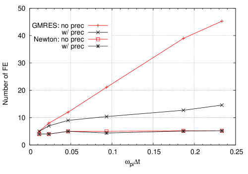
Figure 2: The performance of the JFNK solver against the timestep, with $L=100$, $N_{x}=128$, $N_{pc}=1000$, and $m_{i}/m_{e}=1836$. The number of function evaluations are well controlled by the preconditioner over a large range of $\Delta t$.

For bounded $N_{FE}$, Eq. 18 predicts that the actual CPU time should be largely insensitive to the timestep size. This is confirmed in Fig. 3, which shows the CPU performance of a series of computations with a fixed simulation time-span. Clearly, the total CPU time is essentially independent of $\Delta t$ with preconditioning (but not without). Also, both with and without preconditioning, the average particle pushing time, which is the average CPU time used for all particle pushes during the simulation time-span, saturates for large enough time steps (e.g. $v_{the}\Delta t>1\sim 10\Delta x$), indicating that we have reached an asymptotically large time step. Even though the CPU performance of the preconditioned solver is independent of $\Delta t$, the use of larger timesteps is beneficial for the following reasons. Firstly, the orbit-averaging performed to obtain the plasma current density helps with noise reduction, as it provides the time average of many samplings per particle [26]. Secondly, the operational intensity (computations per memory operation) per particle orbit increases with the timestep, which helps enhance the computing performance (or efficiency) and offset communication latencies in the simulation [17].

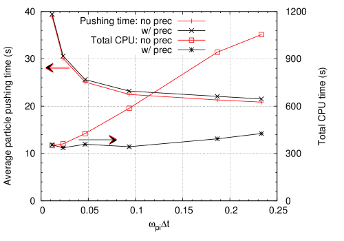
Figure 3: Overall CPU performance as a function of timestep, comparing the unpreconditioned and preconditioned solvers in terms of the average particle pushing time (obtained by the total CPU time divided by the average number of iterations) (left) and wall clock CPU time (right). $L=100$, $N_{x}=128$, $m_{i}/m_{e}=1836$, and the time-span is fixed at 4.67$\omega_{pi}^{-1}$ for all computations.

The performance of the preconditioner vs. the electron-ion mass ratio for both uniform and non-uniform meshes is shown in Tables 1 and 2. To make a fair comparison, both uniform and non-uniform meshes have the same finest mesh resolution, which locally resolves the Debye length. From the tables it is clear that similar performance gains of the preconditioned solver vs. the unpreconditioned one are obtained for both uniform and non-uniform meshes. The dependence of the GMRES performance on the mass ratio is much weaker with the preconditioner: as the mass ratio increases by a factor of 100, the GMRES iteration count increases by a factor of 5 without the preconditioner, vs. a factor of 2 with the preconditioner. Although not completely independent of the mass ratio, the solver behavior is consistent with the asymptotic analysis made in Sec. 5.4.

Table 1: Solver performance with and without the fluid preconditioner for the IAW case with $L=100$, $N_{x}=512$, and $N_{pc}=1000$ on a uniform mesh. For all the test cases, $\Delta t=0.1\omega_{pi}^{-1}$. The Newton and GMRES iteration numbers are obtained by an average over 20 timesteps. For all the runs, we have kept the ion and electron temperature constant.

$m_{i}/m_{e}$	no preconditioner		with preconditioner
	Newton	GMRES	Newton	GMRES
100	4	8	4	7
1600	5	21.2	4	10.1
10000	5.8	50.1	5.5	13.5

Table 2: Solver performance with and without the fluid preconditioner for the IAW case with the non-uniform mesh ($N_{x}=64$ and the smallest mesh size 0.2).

$m_{i}/m_{e}$	no preconditioner		with preconditioner
	Newton	GMRES	Newton	GMRES
100	4	7.6	4	7
1600	5	21.3	5.1	12.1
10000	5.8	48.6	5.3	16.5

The impact of the domain length in the solver performance is shown in Fig. 4. Clearly, the solver performance remains fairly insensitive to the domain length both with and without the preconditioner, even though the domain length varies from 10 to 1000 Debye lengths. This is consistent with the condition number analysis in Eq. 38. The impact of the preconditioner in the number of GMRES iterations is expected for the time step chosen.

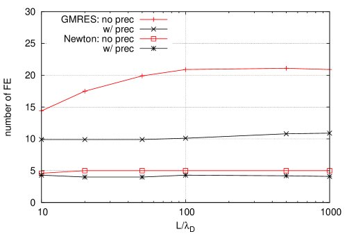
Figure 4: Solver performance as a function of the domain size, with $N_{x}=64$, $N_{pc}=1000$, $\Delta t=0.1\omega_{pi}^{-1}$.

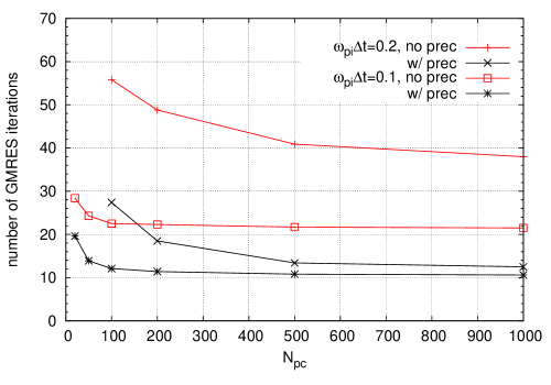
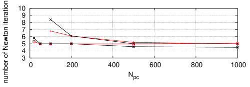
Figure 5: NFE of GMRES and Newton iterations as a function of average number of particles per cell for a domain size $L=100$ with $N_{x}=128$ uniformly distributed cells.

The impact of the number of particles in the performance of the solver is shown in Fig. 5, which depicts the iteration count of both Newton and GMRES vs. the number of particles. The timestep is varied by a factor of two, corresponding to about one-tenth and one-fifth of the inverse ion plasma frequency ($\omega_{pi}^{-1}$). As expected, the solver performs better with smaller timesteps and with larger number of particles. The number of linear and nonlinear iterations increases as the number of particles decreases. This behavior is likely caused by the increased interpolation noise associated with fewer particles: the noise in charge density results in fluctuations in the self-consistent electric field, making the Jacobian-related calculations less accurate, thus delaying convergence. The preconditioner seems to ameliorate the impact of having too few particles on the performance of the algorithm, thus robustifying the nonlinear solver.

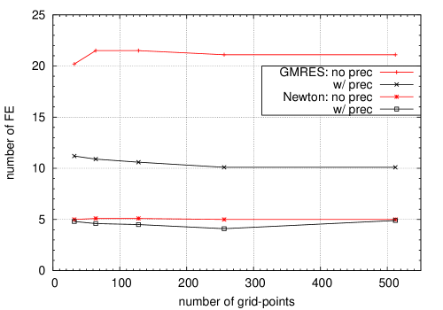
Figure 6: Solver performance vs. the number of grid-points $N_{x}$ for $\omega_{pi}\Delta t=0.093$, $L=100\lambda_{D}$, and $N_{pc}=1000$.

The impact of the number of grid points on the solver performance is shown in Fig. 6 for $\omega_{pi}\Delta t=0.093$, $L=100\lambda_{D}$, and $N_{pc}=1000$. We see that the linear and nonlinear iteration count remains fairly constant with respect to $N_{x}$, with and without preconditioning. This is consistent with the condition number result in Eq. 38 (which is independent of the wavenumber). However, despite the fact that the number of iterations is virtually independent of the number of grid points, the CPU time grows significantly with it. Figure 7 shows that the computational cost scales as $N_{x}^{2}$ for $N_{x}$ large enough. The reason is two-fold. On the one hand, since we keep the number of particles per cell fixed, the computational cost of pushing particles increases proportionally with the number of grid points. On the other hand, as we refine the grid, the cost per particle increases because particles have to cross more cells (for a given timestep). In multiple dimensions, the particle orbit will sample $N^{1/d}$ cells on average, for large enough $N$ (or $\Delta t$), with $N$ and $d$ denoting the total number of grid points and dimensions, respectively. Hence, the cost of particle crossing will scale as $N^{1/d}$, and the computational cost will scale as $N^{1+1/d}$. In this sense, the 1D configuration is the least favorable.

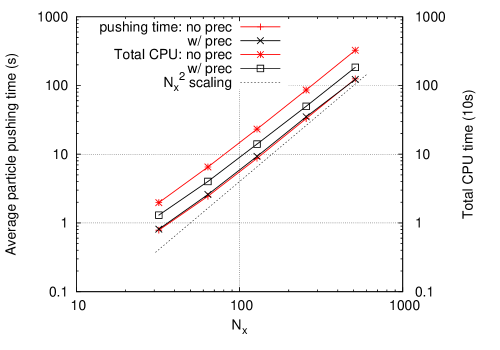
Figure 7: The performance of the JFNK solver against the number of grid-points, with $N_{pc}=1000$. The average particle pushing time is shown on the left and total CPU time for a total time-span $80$ is shown on the right. Both particle pushing time and total CPU time scale as $N_{x}^{2}$ for large enough $N_{x}$.

The performance of the implicit PIC solver vs. the explicit PIC one is compared in Fig. 8, which depicts the CPU speedup vs. $k\lambda_{D}$. For this test, we choose $m_{i}/m_{e}=1836$, $\Delta t=0.1\omega_{pi}^{-1}$, and $N_{pc}=1000$. In the implicit tests, the number of grid-points is kept fixed at $N_{x}=32$ as $L$ increases with $k=2\pi/L$. In the explicit computations, $\Delta x\simeq 0.3\lambda_{D}$ is kept constant for stability, and therefore the number of grid-points increases with $L$. Both implicit and explicit tests employ a uniform mesh. We monitor the scaling power index of Eq. 18 with and without the preconditioner. We test the performance with a large implicit timestep (about 40 times larger than the explicit timestep). The scaling index is found to be $\sim 1.86$ for small domain sizes, close to the expected value of 2. As $L$ increases, the scaling index becomes $\sim 1$. The scaling index turns at $k\lambda_{D}\sim\sqrt{m_{e}/m_{i}}\sim 0.025$, as predicted by Eq. 18. The estimated scaling index of 2 would be recovered if one increased the timestep proportionally to $L$, but this would result in timesteps too large with respect to $\omega_{pi}^{-1}$. Overall, these results are in very good agreement with our simple estimates. The preconditioned solver gains about a factor of two compared to the un-preconditioned one, insensitively to $k\lambda_{D}$, which is consistent with the results depicted in Fig. 4. We see that for $k\lambda_{D}<10^{-3}$, the implicit scheme delivers speedups of about three orders of magnitude vs. the explicit approach, while remaining exactly energy- and charge-conserving.

The setup in Fig. 8 employs a uniform mesh. However, sometimes it is necessary to resolve the Debye length locally, e.g. at a shock front or a boundary layer near a wall. In this case, using a non-uniform mesh is advantageous [20]. We test the performance of the preconditioner on a non-uniform mesh for a nonlinear ion acoustic shock wave, as setup in Ref. [20]. Specifically, we use $L=100\lambda_{D}$, $N_{pc}=2000$, $N_{x}=64$, and $\Delta t=0.1\omega_{pi}^{-1}$ for 20 timesteps. The minimum resolution is $\Delta x=0.5\lambda_{D}$ at the shock location (as in [20], we perform the simulation in the reference frame of the shock). With a nonlinear tolerance $\epsilon_{r}=2\times 10^{-4}$, we have found that, with preconditioning, the average number of Newton and GMRES iterations is 3 and 10.1, respectively, compared to 3.6 and 23 without preconditioning. The performance gain in the linear solve is about factor of two, comparable to that obtained for a uniform mesh with similar problem parameters. Similar performance gains are found with tighter nonlinear tolerances: for $\epsilon_{r}=10^{-8}$, we find 5.1 Newton and 46.6 GMRES iterations without preconditioning, vs. 5 and 20.5 with it.

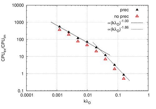
Figure 8: The implicit PIC solver performance compared with the explicit scheme. The performance gain increases with the domain size. For the parameters used, the performance gain of the implicit solver is enhanced by the preconditioner by about a factor of 2.

7 Conclusions

This study has focused on the development of a preconditioner for a recently proposed fully implicit, JFNK-based, charge- and energy-conserving particle-in-cell electrostatic kinetic model [9]. In the reference, it was found that, for large enough implicit time steps $\Delta t$, the potential implicit-to-explicit CPU speedup scaled as $\frac{1}{N_{FE}(k\lambda_{D})^{d}}$, with $N_{FE}$ the number of function evaluations per time step, and $k\lambda_{D}\propto\lambda_{D}/L$. Thus, large speedups are expected when $k\lambda_{D}\ll 1$ provided that $N_{FE}$ is kept bounded. While the CPU speedup does not scale directly with $\Delta t$, the use of large $\Delta t$ is advantageous to maximize operational intensity [17] (i.e., to maximize floating point operations per byte communicated), and to control numerical noise via orbit averaging [26].

We have targeted a preconditioner based on an electron fluid model, which is sufficient to capture the stiffest time scales, and thus enable the use of large implicit time steps while keeping the number of function evaluations bounded. The performance of the preconditioned kinetic JFNK solver has been analyzed with various parametric studies, including time step, mass ratio, domain length, number of particles, and mesh size. The number of function evaluations is found to be insensitive against changes in all of these, delivering a robust nonlinear solver. The CPU time of the implicit PIC solver is found to be insensitive to the time step (as expected), but to scale with the square of the number of mesh points in 1D. This scaling is due to the number of particles per cell being kept constant, and to the number of particle crossings increasing linearly with the mesh resolution. The latter scaling will be more benign in multiple dimensions, as particle orbits remain one-dimensional. Speedups of about three orders of magnitude vs. explicit PIC are demonstrated when $\lambda_{D}\ll L$ (i.e., in the quasineutral regime). Based on the speedup prediction in [9], more dramatic speedups are expected in multiple dimensions.

We conclude that the proposed algorithm shows much promise for extension to multiple dimensions and to electromagnetic simulations. This will be the subject of future work.

Acknowledgments

This work was partially sponsored by the Office of Fusion Energy Sciences at Oak Ridge National Laboratory, and by the Los Alamos National Laboratory (LANL) Directed Research and Development Program. This work was performed under the auspices of the US Department of Energy at Oak Ridge National Laboratory, managed by UT-Battelle, LLC under contract DE-AC05-00OR22725, and the National Nuclear Security Administration of the U.S. Department of Energy at Los Alamos National Laboratory, managed by LANS, LLC under contract DE-AC52-06NA25396.

References

- [1] C. Birdsall and A. Langdon, Plasma Physics via Computer Simulation. New York: McGraw-Hill, 1985.
- [2] R. Hockney and J. Eastwood, Computer Simulation Using Particles. Bristol, UK: Taylor & Francis, Inc, 1988.
- [3] R. J. Mason, “Implicit moment particle simulation of plasmas,” J. Comput. Phys., vol. 41, no. 2, pp. 233 – 44, 1981.
- [4] J. Brackbill and D. Forslund, “An implicit method for electromagnetic plasma simulation in two dimensions,” Journal of Computational Physics, vol. 46, p. 271, 1982.
- [5] A. Friedman, A. B. Langdon, and B. I. Cohen, “A direct method for implicit particle-in-cell simulation,” Comments on plasma physics and controlled fusion, vol. 6, no. 6, pp. 225 – 36, 1981.
- [6] A. Friedman, S. Parker, S. Ray, and C. Birdsall, “Multi-scale particle-in-cell plasma simulation,” Journal of Computational Physics, vol. 96, no. 1, pp. 54–70, 1991.
- [7] B. I. Cohen, A. B. Langdon, D. W. Hewett, and R. J. Procassini, “Performance and optimization of direct implicit particle simulation,” J. Comput. Phys., vol. 81, no. 1, pp. 151 – 68, 1989.
- [8] W. Taitano, D. Knoll, L. Chacón, and G. Chen, “Development of a consistent and stable fully implicit moment method for vlasov-ampére particle-in-cell (pic) system,” SIAM J. Sci. Comput., 2013. In press.
- [9] G. Chen, L. Chacón, and D. C. Barnes, “An energy- and charge-conserving, implicit, electrostatic particle-in-cell algorithm,” Journal of Computational Physics, vol. 230, pp. 7018–7036, 2011.
- [10] S. Markidis and G. Lapenta, “The energy conserving particle-in-cell method,” Journal of Computational Physics, vol. 230, no. 18, pp. 7037–7052, 2011.
- [11] D. A. Knoll and D. E. Keyes, “Jacobian-free Newton–Krylov methods: a survey of approaches and applications,” Journal of Computational Physics, vol. 193, no. 2, pp. 357–397, 2004.
- [12] P. Degond, F. Deluzet, L. Navoret, A.-B. Sun, and M.-H. Vignal, “Asymptotic-Preserving Particle-In-Cell method for the Vlasov-Poisson system near quasineutrality,” J. Comput. Phys., vol. 229, pp. 5630–5652, 2010.
- [13] O. Christensen, Functions, spaces, and expansions: mathematical tools in physics and engineering. Birkhauser, 2010.
- [14] S. E. Parker, A. Friedman, S. L. Ray, and C. K. Birdsall, “Bounded multi-scale plasma simulation: Application to sheath problems,” Journal of Computational Physics, vol. 107, pp. 388 – 402, 1993.
- [15] A. B. Langdon, “Analysis of the time integration in plasma simulation,” J. Comput. Phys., vol. 30, no. 2, pp. 202 – 21, 1979.
- [16] G. Chen and L. Chacón, “An analytical particle mover for the charge-and energy-conserving, nonlinearly implicit, electrostatic particle-in-cell algorithm,” Journal of Computational Physics, vol. 247, no. 15, pp. 79–87, 2013.
- [17] G. Chen, L. Chacón, and D. C. Barnes, “An efficient mixed-precision, hybrid CPU-GPU implementation of a nonlinearly implicit one-dimensional particle-in-cell algorithm,” Journal of Computational Physics, vol. 231, no. 16, pp. 5374–5388, 2012.
- [18] C. T. Kelley, Iterative methods for optimization, vol. 18. Society for Industrial and Applied Mathematics, 1987.
- [19] R. S. Dembo, S. C. Eisenstat, and T. Steihaug, “Inexact Newton methods,” SIAM J. Numer. Anal., vol. 19, no. 2, p. 400, 1982.
- [20] L. Chacón, G. Chen, and D. C. Barnes, “A charge and energy-conserving implicit, electrostatic particle-in-cell algorithm on mapped computational meshes,” Journal of Computational Physics, vol. 233, pp. 1–9, 2013.
- [21] F. F. Chen, Introduction to Plasma Physics and controlled Fusion. New York: Plenum Press, 1984.
- [22] J. Jackson, “Longitudinal plasma oscillations,” Journal of Nuclear Energy. Part C, Plasma Physics, Accelerators, Thermonuclear Research, vol. 1, no. 4, p. 171, 1960.
- [23] N. Krall, “What do we really know about collisionless shocks?,” Advances in Space Research, vol. 20, no. 4, pp. 715–724, 1997.
- [24] R. Fernsler, S. Slinker, and G. Joyce, “Quasineutral plasma models,” Physical Review E, vol. 71, no. 2, p. 026401, 2005.
- [25] J. Williamson, “Initial particle distributions for simulated plasma,” Journal of Computational Physics, vol. 8, no. 2, pp. 258–267, 1971.
- [26] B. I. Cohen, R. P. Freis, and V. Thomas, “Orbit-averaged implicit particle codes,” J. Comput. Phys., vol. 45, no. 3, pp. 345–366, 1982.