A water-like model under confinement for hydrophobic and hydrophilic particle-plate interaction potentials

Abstract

Molecular dynamic simulations were employed to study a water-like model confined between hydrophobic and hydrophilic plates. The phase behavior of this system is obtained for different distances between the plates and particle-plate potentials. For both hydrophobic and hydrophilic walls there are the formation of layers. Crystallization occurs at lower temperature at the contact layer than at the middle layer. In addition, the melting temperature decreases as the plates become more hydrophobic. Similarly, the temperatures of maximum density and extremum diffusivity decrease with hydrophobicity.

I Introduction

Bulk water presents a peculiar complexity on its properties. While in most materials the decrease of the temperature results in a monotonic increase of the density, the water, at ambient pressure, has a maximum in its density at $4^{o}C$ [1, 2, 3]. Furthermore, for usual liquids the response functions increase with the increase of temperature, while water exhibits an anomalous increase of compressibility  [4, 5] between $0.1$ MPa and $190$ MPa and, at atmospheric pressure, an increase of isobaric heat capacity upon cooling [6, 7]. The anomalous behavior of water are not only related with thermodynamic functions, the diffusion coefficient for water has a maximum at $4^{o}C$ for $1.5\;atm$ [3, 8], whereas for normal liquids it increases with the decrease of pressure. The anomalies have been explained in the framework of the existence of a liquid-liquid phase transition ending in a second critical point. This critical point is, however, hidden in a region of the pressure-temperature phase diagram where homogeneous nucleation takes place, and the two liquid phases do not equilibrate [9].

The difficulty of finding the liquid-liquid critical point has been circumvent by experiments performed in confined systems. In these systems the presence of criticality in the bulk has been associated with a dynamic transition between liquids of different viscosities [10, 11, 12, 13].

The study of water in confined geometries is, however, important not only to understand its anomalous properties but also to learn about essential processes to the existence of life, like enzymatic activity of proteins [14, 15, 16]. Confined water plays an important role in many other areas like chemistry, engineering and geology. For these systems is very important to understand the effect in the pressure-temperature phase diagram of the size of the confinement and the hydrophobicity of the wall.

Experiments with water in confined geometries employing NMR [17, 18] and X-ray diffraction [19, 20] show two complementary important findings. First, the pore size has important influence on the freezing and melting temperature. Next, the freezing in these systems is not uniform. Water form layers inside the pores [21, 22, 23, 24] that do not freeze at the same temperature [25] but the middle layers crystallize before the wall layers [21, 24].

Less clear than the pore size effect is the water-wall interaction effect on the melting temperature. Experimental studies show contradictory results. While Akcakayiran et al. [26] using calorimetry studies of water in pores with phosphonic, sulfonic and carboxylic acids show that the melting temperature is not affected by the change of surface, Deschamps et al. [22] and Jelassi et al. [27] show that for water confined in hydrophobic nanopores the liquid states persists to temperatures lower than in bulk and in hydrophilic confinement. These observations are confirmed by X-ray and neutron diffraction [27, 28].

Simulations agree with the experiments in two points. First, the melting temperature of confined water decreases as the system becomes more restrict by decreasing the pore size or distance between plates [29, 30]. Second, the system forms layers [31, 32, 33] where not all the confined water crystallizes [34, 30]. The crystallized layer along the wall is in contact with a pre-wetting liquid layer and some systems present the formation of layers where water just crystallizes partially [34, 35, 36, 37].

Simulations also show controversial results for the effect of hydrophobicity in the melting temperature. While results for SPC/E water show that the melting temperature for hydrophobic plates is lower than the bulk and higher than for hydrophilic walls, for mW model no difference between the melting temperature due to the hydrophobicity [30] is found.

In addition to the melting line, other thermodynamic properties have been explored by simulations. In confined systems the TMD occurs at lower temperatures for hydrophobic confinement [34, 35] and at higher temperatures for hydrophilic confinement [38] when compared with the bulk. The diffusion coefficient, $D$, in the direction parallel to the plates exhibit an anomalous behavior as observed in bulk water. However the temperatures of the the maximum and minimum of $D$ are lower than in bulk water [35]. In the direction perpendicular to the plates, no diffusion anomalous behavior is observed [39].

In this paper we propose that many of the properties described above can be explained in the framework of the competition between the particle-particle interaction and the particle-plate interaction potentials. For that purpose, we study a core-softened fluid [40, 41] confined between parallel plates [42]. The particle-plate interaction is then varied from a very hydrophobic to hydrophilic interaction. The pressure and temperature location of the anomalies, melting and layering are compared with the bulk system for the different particle-plate interactions.

The paper is organized as follows: in Sec. II we introduce the model; in Sec. III the methods and simulation details are described; the results are given in Sec. IV; and conclusions are presented in Sec. V.

II The Model

We study systems with $N$ particles of diameter $\sigma$ confined between two fixed plates. These plates are formed by particles of diameter $\sigma$ organized in a square lattice of area $L^{2}$. The center-to-center plates distance is $d^{*}=d/\sigma$. A schematic depiction of the system is shown in Fig. 1.

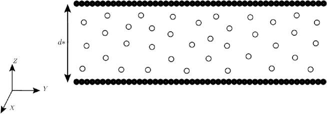
Figure 1: Schematic depiction of the particles confined between two plates separated by a distance $d^{*}$.

The particles of the fluid interact between them through an isotropic effective potential given by

$$\centering\frac{U(r)}{\epsilon}=4\left[\left(\frac{\sigma}{r}\right)^{12}-\left(\frac{\sigma}{r}\right)^{6}\right]+a\exp\left[-\frac{1}{c^{2}}\left(\frac{r-r_{0}}{\sigma}\right)^{2}\right]\;\;.\@add@centering$$ (1)

The first term is a standard Lennard-Jones (LJ) $12-6$ potential with $\epsilon$ depth plus a Gaussian well centered on radius $r=r_{0}$ and width $c$. The parameters used are given by $a=5$, $r_{0}/\sigma=0.7$ and $c=1$. This potential has two length scales with a repulsive shoulder at $r/\sigma\approx 1$ and a very small attractive well at $r/\sigma\approx 3.8$ (Fig. 2). This potential represents in an effective way the tetramer-tetramer interaction forming open and closed structures [43]. The pressure versus temperature phase diagram of this system in the bulk was studied by Oliveira et al. [40, 41]. Density and diffusion anomalous behavior was found for the bulk model.

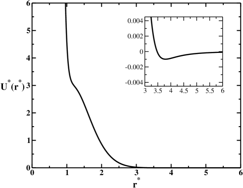
Figure 2: Isotropic effective potential (Eq. 1) of interaction between the water-like particles. The energy and the distances are in dimensionless units, $U^{*}=U/\epsilon$ and $r^{*}=r/\sigma$ and the parameters are $a=5$, $r_{0}/\sigma=0.7$ and $c=1$. The inset shows a zoom in the very small attractive part of the potential.

In order to check the effect of hydrophobicity and confinement, five types of particle-plate interaction potentials were studied namely the repulsive of twenty-forth power (R24), of sixth power (R6), Weeks-Chandler-Andersen (WCA) [44], a weak attractive (WAT) and a strong attractive (SAT). The three first of them are purely repulsive potentials, while the other two have an attractive part. Our simulations are done in reduced units, where $U^{*}=U/\epsilon$ and $r^{*}=r/\sigma$. Three purely repulsive potentials are used: R6, R24 and WCA. The equation of the more repulsive potential (R6) is

$$U_{R6}^{*}=\frac{U_{R6}}{\epsilon}=\left\{\begin{array}[]{ll}A_{1}\left(\sigma/r\right)^{6}+A_{2}\left(r/\sigma\right)-\varepsilon_{1},\qquad r\leq r_{c1}\\ 0,\qquad r>r_{c1}\;,\end{array}\right.$$ (2)

where $r_{c1}=2.0$ and $\varepsilon_{1}=A_{1}\left(\sigma/r_{c1}\right)^{6}+A_{2}(r_{c1}/\sigma)$. For the R24 potential we have

$$U_{R24}^{*}=\frac{U_{R24}}{\epsilon}=\left\{\begin{array}[]{ll}B_{1}\left(\sigma/r\right)^{24}-\varepsilon_{2},\qquad r\leq r_{c2}\\ 0,\qquad r>r_{c2}\;,\end{array}\right.$$ (3)

where $r_{c2}=1.50$ and $\varepsilon_{2}=B_{1}\left(\sigma/r_{c2}\right)^{24}$. The Weeks-Chandler-Andersen Lennard-Jones potential (WCA) is given by

$$U_{WCA}^{*}=\frac{U_{WCA}}{\epsilon}=\left\{\begin{array}[]{ll}U_{{\rm{LJ}}}(r)-U_{{\rm{LJ}}}(r_{c3}),\qquad r\leq r_{c3}\\ 0,\qquad r>r_{c3}\;,\end{array}\right.$$ (4)

where $U_{LJ}(r)$ is a standard 12-6 LJ potential and $r_{c3}=2^{1/6}\sigma$.

Two hydrophilic potentials are analyzed: one weakly hydrophilic, WAT, and another more strong, SAT. The hydrophilic WAT potential is given by

$$U_{WAT}^{*}=\frac{U_{WAT}}{\epsilon}=\left\{\begin{array}[]{ll}C_{1}\left[(\sigma/r)^{12}-(\sigma/r)^{6}\right]+C_{2}\left(r/\sigma\right)-\varepsilon_{4},\qquad r\leq r_{c4}\\ 0,\qquad r>r_{c4}\;,\end{array}\right.$$ (5)

where $r_{c4}=1.5$ and $\varepsilon_{4}=C_{1}\left[(\sigma/r_{c4})^{12}-(\sigma/r_{c4})^{6}\right]+C_{2}(r_{c4}/\sigma)$.

The equation for the SAT potential is

$$U_{SAT}^{*}=\frac{U_{SAT}}{\epsilon}=\left\{\begin{array}[]{ll}D_{1}\left[(\sigma/r)^{12}-(\sigma/r)^{6}\right]+D_{2}\left(r/\sigma\right)-\varepsilon_{5},\qquad r\leq r_{c5}\\ 0,\qquad r>r_{c5}\;,\end{array}\right.$$ (6)

where $r_{c5}=2.0$ and $\varepsilon_{5}=D_{1}\left[(\sigma/r_{c5})^{12}-(\sigma/r_{c5})^{6}\right]+D_{2}(r_{c5}/\sigma)$.

The parameters are illustrated in table 1.

Table 1: Parameters of the particle-plate potentials.

Potential	Parameters values	Parameters values
R6	$A_{1}=4.0$	$A_{2}=0.1875$
R24	$B_{1}=4.0$	$--$
WAT	$C_{1}=1.0$	$C_{2}=0.289$
SAT	$D_{1}=1.2$	$D_{2}=0.0545$

The figure 3 illustrates the particle-plate interaction potentials.

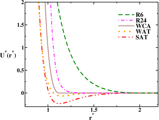
Figure 3: Particle-plate interaction potentials: the three purely repulsive, R6(dashed line), R24(dotted-dashed line), and WCA(solid line), and the attractive, WAT(dotted line) and SAT(double-dotted-dashed line).

III The Methods and Simulation Details

The systems are formed by $N$ particles confined in $z$ direction by two rough plates with area $L^{2}$, located each one at $z=0$ and $z=d$. The position of each plate is fixed. To simulate infinite systems in $x$ and $y$ directions, in order to have the thermodynamic limit, we employed periodic boundary conditions in them. Due to the empty space near to each plates, the distance $d$ between them needs to be corrected to an effective distance [35, 45], $d_{e}$, that can be approach by $d_{e}\approx d-\sigma$. Consequently, the effective density will be $\rho_{e}=N/(d_{e}L^{2})$.

We use molecular dynamic simulations at the NVT-constant ensemble to study the problems suggested. To keep fixed the temperature, we used the Nose-Hoover [46, 47] thermostat, with coupling parameter $Q=2$. The particle-particle interaction was done until the cutoff radius $r_{c}=3.5$ and the potential was shifted in order to have $U=0$ at $r_{c}$.

For all the particle-plate interaction potentials, we study systems with plates separated by distances $d^{*}=d/\sigma=4.2$, $6.0$ and $10.0$. The properties of each case were studied for several temperatures and densities to obtain the full phase diagrams. We use $N=507$ particles for systems at $d^{*}=4.2$ and $d^{*}=6.0$, and $N=546$ particles for systems at $d^{*}=10.0$. The initial configuration was set on solid structure and the equilibrium states reached after $2\times 10^{6}$ steps, followed by $4\times 10^{6}$ simulation run. The time step was $0.001$ in reduced units and the average of the physical quantities were get with $50$ descorrelated samples. We used the behavior of the energy after the equilibrium states and the parallel and perpendicular pressure as function of density to check the thermodynamic stability.

This kind of system requires the division of the thermodynamic averages in the components parallel and perpendicular to the plates. In systems with this geometry, the Helmholtz free energy is given in terms of area, $A=L_{x}L_{y}$, and distance between the plates, $L_{z}$ [48]. Considering the periodic boundary conditions in the plane, the system is extensive just in the area but not in the distance between the plates. Therefore, only the parallel pressure can be regarded as a thermodynamic quantity and it might scale as the experimental pressure. Considering that, we are interested just in the quantities related to parallel direction.

The parallel pressure was calculated using the Virial expression for the $x$ and $y$ directions [35, 39, 48, 34, 49, 45]. The dynamic of the systems was studied by lateral diffusion coefficient, $D_{\parallel}$, related with the mean square displacement (MSD) from Einstein relation,

$$D_{\parallel}=\lim_{\tau\to\infty}\frac{\langle\Delta r_{\parallel}(\tau)^{2}\rangle}{4\tau},$$ (7)

where $r_{\parallel}=(x^{2}+y^{2})^{1/2}$ is the distance between the particles parallel to the plates.

We also studied the structure of the systems by lateral radial distribution function, $g_{\parallel}(r_{\parallel})$. We calculate the $g_{\parallel}(r_{\parallel})$ in specific regions between the plates. An usual definition for $g_{\parallel}(r_{\parallel})$ is

$$g_{\parallel}(r_{\parallel})\equiv\frac{1}{\rho^{2}V}\sum_{i\neq j}\delta(r-r_{ij})\left[\theta\left(\left|z_{i}-z_{j}\right|\right)-\theta\left(\left|z_{i}-z_{j}\right|-\delta z\right)\right].$$ (8)

The $\theta(x)$ is the Heaviside function and it restricts the sum of particle pairs in the same slab of thickness $\delta z=1$. We need to compute the number of particles for each region and the normalization volume will be cylindrical. The $g_{\parallel}(r_{\parallel})$ is proportional to the probability of finding a particle at a distance $r_{\parallel}$ from a referent particle.

All physical quantities are shown in reduced units [50] as

$$d^{*} = \frac{d}{\sigma}$$

$$\tau^{*} = \frac{(\epsilon/m)^{1/2}}{\sigma}\tau$$

$$T^{*} = \frac{k_{B}}{\epsilon}T$$

$$P_{\parallel,\perp}^{*} = \frac{\sigma^{3}}{\epsilon}P_{\parallel,\perp}$$

$$\rho^{*} = \sigma^{3}\rho$$

$$D_{\parallel}^{*} = \frac{(m/\epsilon)^{1/2}}{\sigma}D_{\parallel}\;\;.$$ (9)

IV Results

The Structure

First, we check the effects of decreasing the plates distance and the hydrophobicity in the number of layers of water and its structure. For that purpose we focus in three layer distances $d^{*}=10.0,6.0$ and $4.2$ in which we observe the presence of five, three and two layers respectively for all the particle-plate potentials.

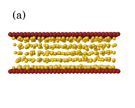
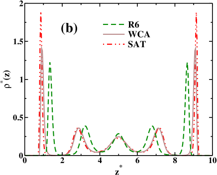
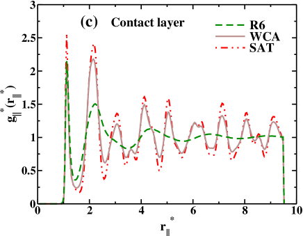
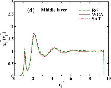
Figure 4: Systems with plates separated by a distance $d^{*}=10.0$ at $\rho^{*}=0.168$ and $T^{*}=0.140$. (a) Snapshot showing the five layers for the WCA case. (b)Transversal density versus $z$ for systems confined by the R6, WCA and SAT potentials. Radial distribution function versus distance for the (c) contact and (d) middle layers. The confinements by the R24 and WAT potentials have similar results than the WCA and are not shown for simplicity.

The figure 4 illustrates the structure for the distance between the plates $d^{*}=10.0$ at $\rho^{*}=0.168$ and $T^{*}=0.140$ only for the three cases R6, WCA and SAT for simplicity. In the figure 4(a) the snapshot shows the structure with five layers (only the WCA for simplicity). In the figure 4(b) the density at the $z$ direction is plotted against $z$, showing that for the attractive potential the contact layer is closer to the plates when compared with the purely repulsive particle-plate potentials. The distance between the layers is arranged to minimize the particle-particle interaction illustrated in the figure 2, while the distance between the plate and the contact layer to minimize the particle-plate interaction. This simple geometrical arrangement is robust for all the potentials and as we shall see below for various plate-plate distances. The figures 4(c) and (d) illustrates the radial distribution functions for the contact and middle layers respectively. While the contact layers show the presence of an amorphous-like structure, the middle layers are liquid. The only case in which both layers are liquids is the repulsive case R6. This result is in agreement with SPC/E simulation of Gallo et al. [51].

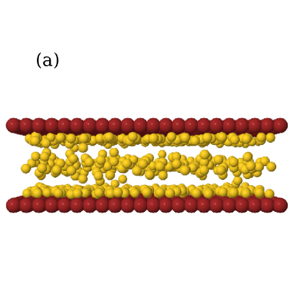
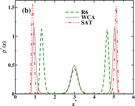
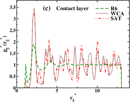
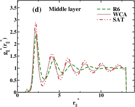
Figure 5: Systems with plates separated by a distance $d^{*}=6.0$ at $\rho^{*}=0.150$ and $T^{*}=0.140$. (a) Snapshot showing the three layers for the WCA case. (b)Transversal density versus $z$ for systems confined by the R6, WCA and SAT potentials. (c) Radial distribution function versus distance for the contact and (d) middle layers. The confinements by the R24 and WAT potentials have similar results than the WCA and are not shown for simplicity.

The figure 5 illustrates the system for plates separated by a distance $d^{*}=6.0$ at $\rho^{*}=0.150$ and $T^{*}=0.140$. In the figure 5(a) the snapshot shows the structure with three layers (only the WCA for simplicity), two contact layers and one middle layer. In the figure 5(b) the density versus $z$ indicates that as the plates becomes more attractive, particles are pushed toward them. The figures 5(c) and (d) show that for $d^{*}=6.0$ the contact layer presents an amorphous-like structure while the middle layer is fluid. This observation is true for all the particle-plate potentials with the exception of the R6 which is fluid at the contact and middle layers.

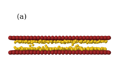
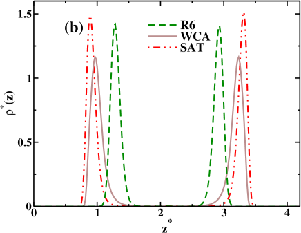
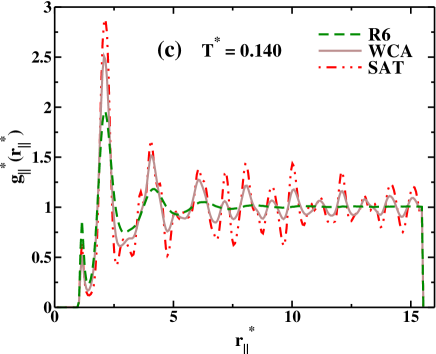
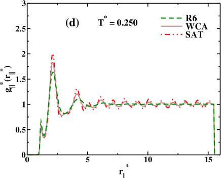
Figure 6: Systems with plates separated by a distance $d^{*}=4.2$ at $\rho^{*}=0.165$. (a) Snapshot showing the two layers for the WCA case at $T^{*}=0.140$. (b)Transversal density versus $z$ for systems confined by the R6, WCA and SAT potentials. Radial distribution function versus distance for one contact layer for (c) $T^{*}=0.140$ and for (d) $T^{*}=0.250$. The confinements by the R24 and WAT potentials have similar results than the WCA and are not shown for simplicity.

For the distance $d^{*}=4.2$ and $\rho^{*}=0.165$ two temperatures were analyzed, $T^{*}=0.140$ and $T^{*}=0.250$. The figure 6(a) shows a snapshot of the system (only for the WCA for simplicity) indicating the presence of two layers. The figure 6(b) shows the density at the $z$ direction. Similarly to the $d^{*}=10$ and $6.0$ cases the mainly effect of hydrophobicity is to have the two layers closer to the wall than in the case of the hydrophilic wall. The figure 6(c) and (d) shows the radial distribution function for two temperatures $T^{*}=0.140$ and $T^{*}=0.250$ respectively. While $T^{*}=0.140$ shows an amorphous-like structure for the WCA and SAT potentials, $T^{*}=0.250$ is liquid, indicating that the system melts at an intermediate temperature. The R6 potentials exhibits a liquid-like behavior for both temperatures.

In all the cases showed above, the purely repulsive potential R6 has no crystalline layer. This suggests that the crystallization in this case occur at higher pressures. In order to check that, the case at $d^{*}=10.0$ is analyzed for $\rho^{*}=0.210$ in comparison with $\rho^{*}=0.168$, shown in figure 4. In the figure 7 (a) the transversal density versus $z$ is shown for a system with plates separated by $d^{*}=10.0$ at $\rho^{*}=0.210$ and $T^{*}=0.140$, showing the five layers formed, and in (b), we have the $g_{||}(r_{||})$ of the contact and the middle layers. Both layers represent amorphous states and, besides that, it is possible to see that the middle layer is smoothly more structured than the contact layer. This is an interesting and an important observation because some experimental results say that the middle layer crystallizes before than the contact layer [21, 24]. This result is obtained just for the R6 potential, which lead us again to the conclusion that this potential is the best to reproduce the structure related in some experiments for the hydrophobicity.

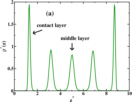
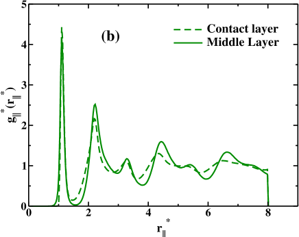
Figure 7: Transversal density versus $z$ in (a) and $g_{||}(r_{||})$ in (b) for $d^{*}=10.0$, $\rho^{*}=0.209$ and $T^{*}=0.140$. The middle layer is more structured than the contact layer, which is in agreement with some experimental results for hydrophobic confinement.

Our results, comparing the different potentials and plates distances, indicate that the hydrophobicity has little effect in number of layers that is defined by the distance $d^{*}$ between the plates. The crystallization of the contact layer, however, seems to be dependent both of the particle-plate interaction and of the distance between the plates. In order to explore in detail the process of crystallization of the contact layer we analyze the phase behavior of the confined systems for the R6 and SAT potentials. The figure 8 shows the phase behavior of the systems confined by the (a) R6 and (b) SAT potentials at $T^{*}=0.140$. The open circles indicate liquid-state points while filled squares indicate solid-state points. An approximate boundary between the liquid and solid-states are indicated by the black lines in the figures. For this specific temperature, our results suggest that the melting pressure decreases with $d^{*}$ for the hydrophobic potentials and increases with $d^{*}$ for the hydrophilic potentials. This result is consistent with the liquid-gas observations in the SPC/E confined model [29].

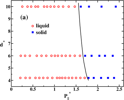
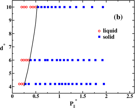
Figure 8: Distance $d^{*}$ between the plates as function of density of the system for (a) R6 and (b) SAT confinements at $T^{*}=0.140$. The open circles indicate liquid-state points while filled squares indicate solid-state points. The black lines are an approximate boundary between the liquid and solid-states.

The figure 9 shows the melting temperature of the systems at $\rho^{*}=0.176$ for (a) repulsive potentials (R6, R24 and WCA) and for (b) attractive potentials (WAT and SAT). For temperatures $T^{*}>T^{*}_{m}$, all the system are in liquid-state, while for $T^{*}<T^{*}_{m}$ a crystallization occurs at least for the contact layers. The SAT potential crystallizes more easily than the other cases and has a peculiar behavior with the distance $d^{*}$ between the plates. The crystallization for the SAT potentials occurs more easily as the degree of confinement increases (decreasing of $d^{*}$), while other cases show the opposite behavior. Our results are in agreement with simulations and experiments for water confined in hydrophobic and hydrophilic nanopores [30, 22].

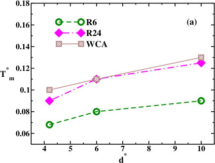
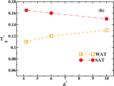
Figure 9: Melting temperature as function of separation $d^{*}$ between the plates for (a) repulsive (R6, R24 and WCA) and (b) attractive (WAT and SAT) potentials. Systems at $\rho^{*}=0.176$.

Diffusion and density anomalous behavior

In this subsection we analyze the effect of hydrophobicity and changing the plates distances in the location in the pressure-temperature phase diagram of the diffusion and density anomalies. The Figure 10 (a) shows a comparison between the mean square displacement parallel to the plates at $d^{*}=4.2$, $\rho^{*}=0.165$ and $T^{*}=0.250$. The plot shows that the mobility is higher for hydrophobic than hydrophilic particle-plate interactions. This result is consistent with the layer density illustrated in the Figure 6(b) that shows that attractive particle-plate interactions leave more space for the layers. In the Figure 10(b) the diffusion coefficient is shown as a function of the density for $d^{*}=4.2$ and WCA confining potential, illustrating the presence of a region where diffusion increases with the increase of the density what is defined as diffusion anomalous region (region between the dashed lines). This anomalous behavior is also present for the other distances $d=6.0$ and $10.0$ and other particle-plate potentials.

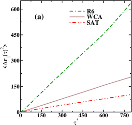
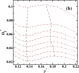
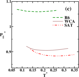
Figure 10: Systems for $d^{*}=4.2$, $\rho^{*}=0.165$ and $T^{*}=0.250$. (a) Mean square displacement versus time for R6, WCA and SAT potentials. (b) Diffusion coefficient versus density for the WCA potential at fixed temperatures $T^{*}=0.175$, $0.190$, $0.205$, $0.220$, $0.235$, $0.250$, $0.270$ and $0.320$ from the bottom to the top. (c) Isochore $\rho^{*}=0.165$ at the pressure-temperature phase diagram for R6, WCA and SAT potentials. The R24 and WAT potentials are intermediate cases and are not shown for simplicity.

Next, we test our system for the presence of the temperature of maximum density (TMD). The TMD lines can be found computing $(\partial P_{||}/\partial T)_{\rho}=0$, corresponding to minimum of the isochores. A comparison between the same isochore ($\rho^{*}=0.165$) for each potential is given in the Figure 10 (c) for $d^{*}=4.2$. The temperature of maximum density decreases and its pressure increases as the system becomes more hydrophobic. The pressure increase can be understood in terms of the decrease of effective volume for hydrophobic plates as shown in figure 6(b) with corresponding increase of pressure. The decrease of the TMD with hydrophobicity can be understood as follows. In our effective model the two length scales represent the bond and non-bonding cluster of molecules. As temperature increases the number of clusters with “non-bonding molecules grow while the number of clusters with “bonding” molecules decreases. The TMD is the temperature in which the two distributions become equivalent. In the confined system the wall repulsion favor the “non-bonding length scale and the TMD happens at lower values. The Figure 11 shows the parallel pressure versus temperature phase diagram for (a)-(c) R6, (d)-(f) WCA and (g)-(h) SAT potentials. The dashed lines comprises the diffusion anomaly and the solid lines indicate the density anomaly for each case. For all the cases studied, the hierarchy of the anomalies are observed.

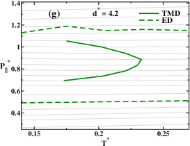
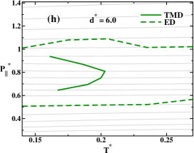
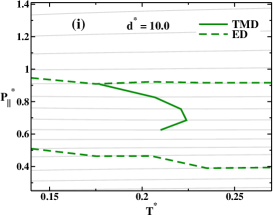
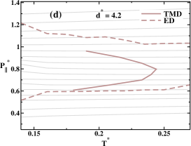
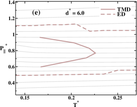
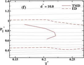
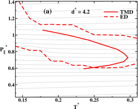
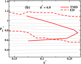
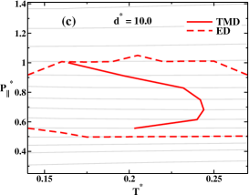
Figure 11: Parallel pressure versus temperature phase diagrams for (a)-(c), R6 (d)-(f) WCA and (g)-(h) SAT potentials. For all the plots the solid line is the TMD line and the dashed line is the extremum diffusion coefficient line. The range of densities are $0.089\leq\rho^{*}\leq 0.182$ for systems at $d^{*}=4.2$, $0.087\leq\rho^{*}\leq 0.176$ for $d^{*}=6.0$ and $0.083\leq\rho^{*}\leq 0.168$ for $d^{*}=10.0$.

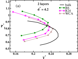
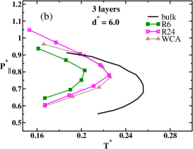
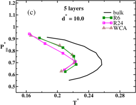
Figure 12: Pressure versus temperature phase diagram illustrating the TMD line for hydrophobic confinement, R6, R24 and WCA potentials, for (a) $d^{*}=4.2$, (b) $d^{*}=6.0$ and (c) $d^{*}=10.0$.

Confirming the scenario we describing above, Figure 12 illustrates the TMD lines for the hydrophobic particle-plate interaction potentials for (a) $d^{*}=4.2$, (b) $d^{*}=6.0$ and (c) $d^{*}=10.0$. The TMD lines are shifted to lower temperatures in relation to bulk system as the distance between the plates is decreased. This result is consistent with atomistic models [35, 34].

Figure 13 shows the TMD lines for the hydrophilic particle-plate interaction potentials for different plates separations. For these cases the TMD moves to higher temperatures when compared to the bulk values as the distance between the plates is decreased. This result is consistent with atomistic models [38].

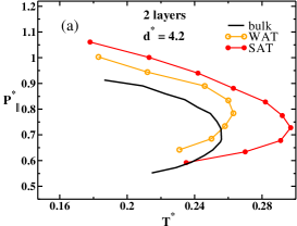
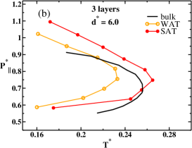
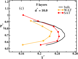
Figure 13: Pressure versus temperature phase diagram illustrating the TMD line for hydrophilic confinement, WAT and SAT potentials, for (a) $d^{*}=4.2$, (b) $d^{*}=6.0$ and (c) $d^{*}=10.0$.

V Conclusions

In this paper we have explored the effect of the confinement in the thermodynamic, dynamic and structural properties of a core-softened potential designed to reproduce the anomalies present in water.

We have shown that both hydrophobic and hydrophilic walls change the melting, the TMD and the extrema diffusivity temperatures. While melting is suppressed by hydrophobic walls, crystallization happens for hydrophilic confinement at higher temperatures if the walls would be attractive enough.

Our results suggest that layering, crystallization and thermodynamic and dynamic anomalies are governed by the competition between the two length scales that characterize our model and the particle-plate interaction length. These results are consistent with atomistic models [29, 30, 37, 35], however due the simplicity of the simulation we were able to explore a large variety of potentials to confirm our assumption that a simple competition between scales not only is able to reproduce the water anomalies but to capture the confinement phase diagram.

References

- [1] R. Waler. Essays of natural experiments. Johnson Reprint, New York, 1964.
- [2] G. S. Kell, J. Chem. Eng. Data 20, 97 (1975).
- [3] C. A. Angell, E. D. Finch, L. A. Woolf and P. Bach, J. Chem. Phys. 65, 3063 (1976).
- [4] R. J. Speedy, and C. A. Angell, J. Chem. Phys. 65, 851 (1976).
- [5] H. Kanno, and C. A. Angell, J. Chem. Phys. 70, 4008 (1979).
- [6] C. A. Angell, M. Oguni, and W. J. Sichina, J. Chem. Phys. 86, 998 (1982).
- [7] E. Tombari, C. Ferrari, and G. Salvetti, Chem. Phys. Lett. 300, 749 (1999).
- [8] F. X. Prielmeier, E. W. Lang, R. J. Speedy, and H.-D. Lüdemann, Phys. Rev. Lett. 59, 1128 (1987).
- [9] P. H. Poole, F. Sciortino, U. Essmann, and H. E. Stanley, Nature (London) 360, 324 (1992).
- [10] L. Liu, S.-H. Chen, A. Faraone, S.-W. Yen, and C.-Y. Mou, Phys. Rev. Lett. 95, 117802 (2005).
- [11] X.-Q. Chu, K.-H. Liu, M. S. Tyagi, C.-Y. Mou, and S.-H. Chen, Phys. Rev. E 82, 020501 (2010).
- [12] S.-H. Chen, F. Mallamace, C.-Y. Mou, M. Broccio, C. Corsaro, A. Faraone, and L. Liu, Proc. Natl. Acad. Sci. USA 103, 12974 (2006).
- [13] F. Mallamace, C. Corsaro, M. Broccio, C. Branca. N. González-Segredo, J. Spooren, S.-H. Chen., and H. E. Stanley, Proc. Natl. Acad. Sci. USA 105, 12725 (2008).
- [14] S.-H. Chen, L. Liu, E. Fratini, P. Baglioni, A. Faraone, and E. Mamontov, Proc. Natl. Acad. Sci. USA 103, 9012 (2006).
- [15] G. Franzese, K. Stokely, X-q. Chu, P. Kumar, M. G. Mazza, S.-H. Chen, and H. E. Stanley, J. Phys.: Condens. Matter 20, 494210 (2008).
- [16] A. Kuffel and J. Zielkiewicz, J. Phys. Chem. B 116, 12113 (2012).
- [17] E. W. Hansen, M. Stöker, and R. Schmidt, J. Chem. Phys. 100, 2195 (1996).
- [18] K. Overloop and L. Van Gerven, J. of Magnet. Res. 101, 179 (1992).
- [19] K. Morishige, and K. Kawano, J. Chem. Phys. 110, 4867 (1999).
- [20] K. Morishige and H. Iwasaki, Langmuir 19, 2808 (2003).
- [21] M. Erko, G. H. Findenegg, N. Cade, A. G. Michette, and O. Paris, Phys. Rev. B 84, 104205 (2011).
- [22] J. Deschamps, F. Audonnet, N. Brodie-Linder, M. Schoeffel, and C. Alba-Simionesco, Phys. Chem. Chem. Phys. 12, 1440 (2010).
- [23] S. Jähnert, F. V. Chávez, G. E. Schaumann, A. Schreiber, M. Schönhoff, and G. H. Findenegg, Phys. Chem. Chem. Phys. 10, 6039 (2008).
- [24] K. Morishige, and K. Nobuoka, J. Chem. Phys. 107, 6965 (1997).
- [25] M.-C. Bellissent-Funel, J. Lal, and L. Bosio, J. Chem. Phys. 98, 4246 (1993).
- [26] D. Akcakayiran, D. Mauder, C. Hess, T. K. Sievers, D. G. Kurth, I. Shenderovich, H. H. Limbach, and G. H. Findenegg, J. Phys. Chem. B 112, 14637 (2008).
- [27] J. Jelassi, T. Grosz, I. Bako, M. -C. Belissent-Funel, J. C. Dore, H. L. Castricum, and R. Sridi-Dorbez , J. Chem. Phys. 134, 064509 (2011).
- [28] M. Sliwinska-Bartkowiak, M. Jazdzewska, L. L. Huang, and K. E. Gubbins, Phys. Chem. Chem. Phys. 10, 4909 (2008).
- [29] N. Giovambattista, P. J. Rossky, and P. G. Debenedetti, J. Phys. Chem. B 113, 13723 (2009).
- [30] E. B. Moore, J. T. Allen, and V. Molinero, J. Phys. Chem. C 116, 7507 (2012).
- [31] R. Zangi, and A. E. Mark, J. Chem. Phys.119, 1694 (2003).
- [32] S. Han, M. Y. Choi, P. Kumar, and H. E. Stanley, Nature Physics 6, 685 (2010).
- [33] J. R. Bordin, A. B. de Oliveira, A. Diehl, and M. C. Barbosa, J. Chem. Phys. 137, 084504 (2012).
- [34] N. Giovambattista, P. J. Rossky, and P. G. Debenedetti, Phys. Rev. Lett. 102, 050603 (2009).
- [35] P. Kumar, S. V. Buldyrev, F. W. Starr, N. Giovambattista, and H. E. Stanley, Phys. Rev. E 72, 051503 (2005).
- [36] P. Gallo, M. Rovere, and E. Spohr, J. Chem. Phys. 113, 11324 (2000).
- [37] E. G. Solveyra, E. de la Llave, D. A. Scherlis, and V. Molinero, J. Phys. Chem. B 115, 14196 (2011).
- [38] S. R.-V. Castrillon, N. Giovambattista, I. A. Aksay, and P. G. Debenedetti, J. Chem. Phys. B 113, 1438 (2009).
- [39] S. Han, P. Kumar, and H. E. Stanley, Phys. Rev. E 77, 030201 (2008).
- [40] A. B. de Oliveira, P. A. Netz, T. Colla, and M. C. Barbosa, J. Chem. Phys. 124, 084505 (2006).
- [41] A. B. de Oliveira, P. A. Netz, T. Colla, and M. C. Barbosa, J. Chem. Phys. 125, 124503 (2006).
- [42] L. B. Krott and M. C. Barbosa, J. Chem. Phys. 138, 084505 (2013).
- [43] M. Chaplin, Sixty-nine anomalies of water, http://www.lsbu.ac.uk/water/anmlies.html, 2013.
- [44] J. D. Weeks, D. Chandler, and H. C. Andersen, J. Chem. Phys. 54, 5237 (1971).
- [45] P. Kumar, F. W. Starr, S. V. Buldyrev, and H. E. Stanley, Phys. Rev. E 75, 011202 (2007).
- [46] W. G. Hoover, Phys. Rev. A 31, 1695 (1985).
- [47] W. G. Hoover, Phys. Rev. A 34, 2499 (1986).
- [48] M. Meyer, and H. E. Stanley, J. Phys. Chem. B 103, 9728 (1999).
- [49] P. Kumar, S. Han, and H. E. Stanley, J. Phys.: Condens. Matter 21, 504108 (2009).
- [50] M. P. Allen, and D. J. Tildesley. Computer Simulations of Liquids (first ed.). Claredon Press, Oxford, 1987.
- [51] P. Gallo and M. A. Ricci and M. Rovere, J. Chem. Phys. 116, 342 (2002).