Directed Ratchet Transport in Granular Crystals

Abstract

Directed-ratchet transport (DRT) in a one-dimensional lattice of spherical beads, which serves as a prototype for granular crystals, is investigated. We consider a system where the trajectory of the central bead is prescribed by a biharmonic forcing function with broken time-reversal symmetry. By comparing the mean integrated force of beads equidistant from the forcing bead, two distinct types of directed transport can be observed —spatial and temporal DRT. Based on the value of the frequency of the forcing function relative to the cutoff frequency, the system can be categorized by the presence and magnitude of each type of DRT. Furthermore, we investigate and quantify how varying additional parameters such as the biharmonic weight affects DRT velocity and magnitude. Finally, friction is introduced into the system and is found to significantly inhibit spatial DRT. In fact, for sufficiently low forcing frequencies, the friction may even induce a switching of the DRT direction.

I Introduction

Granular media are large conglomerations of discrete, solid particles, such as sand, gravel, or powder, with unusual, interesting dynamics Trujillo2011 ; Jaeger1996 ; Luding1995 . A one-dimensional system of spherical beads in a lattice is one of the simplest representation of granular media substrates, wherein each bead represents a grain of material. In this approximation, the position of a particular bead is based on forces resulting from its interaction with its two nearest neighbors Nesterenko2001 . This context has proved especially fruitful for investigating numerous aspects of the nonlinear dynamic response of such bead chain systems Nesterenko2001 ; sen08 ; PGK11 . A particular focal point of emphasis has been on the study of one-dimensional granular crystals. The availability of a wide variety of materials and bead sizes, as well as the tunability of the response within the weakly or strongly nonlinear regime renders such crystals an ideal playground for the investigation of a variety of fundamental concepts ranging from nonlinear waves and discrete breathers to shock waves, defect modes and bifurcation phenomena among many others. However, this tunability also makes these crystals promising candidates for a wide variety of engineering applications such as shock and energy absorbing materials dar06 ; hong05 ; fernando ; doney06 , actuating and focusing devices dev08 ; spadoni10 , and sound scramblers or filters dar05 ; dar05b ; chiara_nature .

One aspect that has not been studied, to the best of our knowledge, in such prototypical granular lattices is that of directed transport via the so-called ratcheting effect. Directed ratchet transport (DRT), is defined as the directed transmission of an entity despite the lack of a net external force acting upon it Hanggi09 ; Rietmann2011 . This phenomenon has been associated with applications in dc current in semiconductors Carlin1965 , the motion of fluxons in Josephson junctions Falo99 ; Falo02 ; Ustinov2004 , Bose-Einstein condensates Rietmann2011 ; Poletti2008 , cold atoms in optical lattices renzoni1 ; renzoni2 , among many others. Furthermore, DRT occurring in granular systems has been associated with the study of molecular motors Julicher1997 . As detailed in Ref. Flach2000 , the emergence of DRT behavior is associated with the breaking of symmetries, which can be achieved by either a reshaping of the system’s potential or by introducing an external forcing Reimann2002 . For instance, DRT is present when a granular material is placed in a vertically vibrating sawtooth surface profile Rapaport:02 . Typically, DRT is studied (for a single particle or a collection of particles) when the external input acts on the system as a whole Falo99 ; Falo02 . Our aim in this work, on the other hand, is to force a single particle to achieve global DRT in the context of granular crystals.

In what follows in section II, we present the basic (Fermi-Pasta-Ulam type) model that is widely accepted as representing the one-dimensional dynamics of a granular crystal Nesterenko2001 ; sen08 ; PGK11 with parameters that are adapted from recent experiments on the field such as Refs. Boechler2010 ; Boechler2012 . We then proceed to use the tunability of the system through actuating one bead within the chain by means of suitable biharmonic forcing that will be the source of our DRT through its induced breaking of time-reversal and half-period time shift symmetries. In particular, in section III, we will propose a biharmonic forcing of the system involving the simplest pair of two frequencies $(p\omega,q\omega)$ relevant for such DRT (i.e., with $p,q$ coprimes and $p+q$ odd), namely $p=1$ and $q=2$ Quintero2010 . In section IV, we will develop diagnostic quantities evaluating the relative magnitude of the clearly discernible in our numerical computations DRT. We will analyze the dependence of the induced asymmetry in the crystal response on both the frequency of the drive $\omega$, as well as on the relative strength of the two terms in the biharmonic forcing, as controlled by the corresponding parameter $\eta$. The former analysis will separate different regimes in our observation of DRT, namely the non-permanent deformation of the crystal that we will refer to as temporal ratcheting and the permanent deformation thereof that we will refer to as spatial ratcheting. The clear distinction between these two regimes is an especially intriguing feature of our current setup. The latter analysis (over $\eta$) will provide a means for optimizing the ensuing transport which can both be theoretically understood and, in principle, experimentally exploited. Finally, we consider in section V, the modification of the above features in the more experimentally realistic setup incorporating dissipation. We find there that the relevant phenomenology is modified dramatically, including even a potential reversal of the direction of the current (for sufficiently low driving frequencies). Finally, in section VI we summarize our findings and present a number of directions for future study.

II Model and Setup

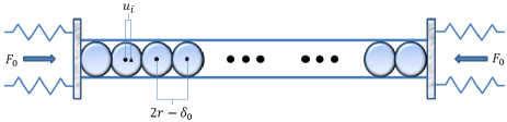
Figure 1: The bead-lattice system with precompression force $F_{0}$ delivered by springs connected to walls on both ends of the lattice. The small circular dots represent the location of the center of each bead at its equilibrium position. Notice that, because of the initial displacement due to precompression, the equilibrium distance between two beads is $2r-\delta_{0}$. The triangle represents the position of the center of the $i$th bead after displacement $u_{i}$.

To ensure that the beads remain in contact, we consider a horizontal lattice that is precompressed on both ends with a force $F_{0}$ resulting in a static bead displacement $\delta_{0}$ (see Fig. 1). The existence of the precompression also serves to ensure that a linear spectrum of excitations exists in the lattice (see details below). With these considerations, based on the Hertzian law of spherical point contacts, a system comprised of $N$ identical beads can be described by the following Newtonian equation Nesterenko2001 :

$$m\ddot{u}_{i}=A[\delta_{0}+u_{i-1}-u_{i}]_{+}^{\frac{3}{2}}-A[\delta_{0}+u_{i}-u_{i+1}]_{+}^{\frac{3}{2}}$$ (1)

where $[Y]_{+}={\rm max}\left\{0,Y\right\}$, $m$ is the bead mass, $u_{i}$ is the displacement of the center of the $i$th bead from its equilibrium position, and $A$ is the Hertzian constant calculated as

$$A\equiv\frac{2E\sqrt{r}}{3\sqrt{2}(1-\nu^{2})},$$ (2)

where $r$, $E$, $\nu$ are, respectively, the bead’s radius, Young’s elastic modulus, and Poisson’s ratio. The static displacement is $\delta_{0}=\left(\frac{F_{0}}{A}\right)^{\frac{2}{3}}$. In line with the experiments of Refs. Boechler2010 ; Boechler2012 , the parameter values listed in Table 1 were used.

Table 1: Default Parameters for Bead-Lattice System.

Parameter	Symbol	Default Value
Mass	$m$	28.84 g
Radius	$r$	9.53 mm
Poisson’s ratio	$\nu$	0.3
Young’s modulus	$E$	0.193 $\frac{g}{{\rm mm}\,\mu{\rm s}}$
Precompression force	$F_{0}$	5 N

As we will show later, a critical factor affecting the presence/type of DRT is the acoustic phonon band cutoff frequency. Plane wave solutions to the system follow the dispersion relation $\bar{\nu}(\alpha)^{2}={\frac{3}{2}A\sqrt{\delta_{0}}\sin^{2}(\pi\delta_{0}\alpha)}/({m\pi^{2}})$ Brillouin1946 , where $\alpha$ is the wave number and $\bar{\nu}$ is the temporal frequency. We see that this relationship is periodic (with period ${1}/{\delta_{0}}$) and that there is a cutoff frequency $\bar{\nu}_{c}$, above which plane wave solutions cannot propagate. The maximal frequency value occurs at the boundaries of the $-\frac{1}{2\delta_{0}}\leq\alpha\leq\frac{1}{2\delta_{0}}$ interval, which correspond to the smallest allowable wavelength. Substituting $\alpha=\pm\frac{1}{2\delta_{0}}$ into the dispersion relation yields the cutoff frequency,

$$\bar{\nu}_{c}=\frac{1}{\pi}\sqrt{\frac{\frac{3}{2}A\sqrt{\delta_{0}}}{m}}.$$ (3)

Therefore, $0<\bar{\nu}<\bar{\nu}_{c}$ defines the range of propagating frequencies, called the acoustic band. Frequencies $\bar{\nu}>\bar{\nu}_{c}$ lie within the band gap and cannot propagate through the lattice as plane waves. With the parameter values given in Table 1, we have $\bar{\nu}_{c}=6.42$ kHz. In terms of angular frequency, $\omega_{c}=2\pi\bar{\nu}_{c}=$ 40.31 ${\mathrm{rad}}/{\mathrm{ms}}$, which is the critical frequency used from this point forward. Notice that all the frequencies that will be mentioned hereafter will be measured in ${\mathrm{rad}}/{\mathrm{ms}}$.

III Biharmonic Forcing

Typically, DRT behavior is observed in the velocity of a single particle or in that of a coherent structure such as a solitary wave Rietmann2011 ; Flach2000 ; Reimann2002 ; Quintero2010 ; Jesus10 . In the case of the granular crystal though, DRT will be observed (and examined) throughout the system as a whole. Consider a lattice where each bead begins at its equilibrium position with no initial velocity. To introduce energy into the system, the $i^{*}$th bead, located at the center of the lattice, is controlled by the following biharmonic, periodic function

$$u_{i^{*}}(t)=a\left[\eta\sin(\omega(t+\phi))+(1-\eta)\sin(2\omega(t+\phi))\right],$$ (4)

where $t$ is time, $a$ is the amplitude, $\omega$ is the frequency, $\eta$ is the biharmonic weight, and $\phi$ is a phase. To maintain uniformity on each side of $i^{*}$th bead, we assume $N$ is odd. The motivation for choosing to control the displacement of the central bead is that we envisage the possibility of doing experimental DRT studies in the future where the position of the central bead will be controlled by an actuator. An essential characteristic of this functional form is that it has a zero-integral over one period, indicating that the function is not biased in any direction. In other words, the $i^{*}$th bead’s temporal center of mass, relative its equilibrium position, is zero. Consequently, any directed behavior observed must be attributed to DRT rather than a preferential direction for the input. It is relevant to note that the prescription of the motion of the $i^{*}$th bead is tantamount to introducing a force, with the same characteristics, into its nearest neighbors through the equations of motion (1).

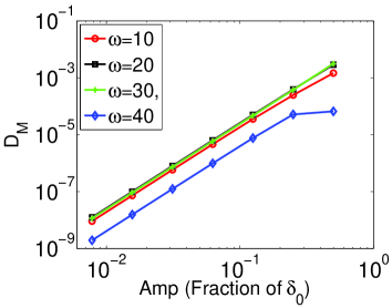
Figure 2: DRT magnitude vs. forcing amplitude $a$. The default parameters in Tables 1 are used with $\eta={4}/{9}$ and $\phi$ averaged over 16 values.

For $\eta=\{0,1\}$ each bead orbit on one side of the lattice corresponds directly to an orbit on the other side of the lattice traveling in the opposite direction, translated by a half-period delay. These orbits exactly cancel each other out and thus there is no DRT. However, when $\eta\in(0,1)$, the symmetry of $u_{i^{*}}(t)$ is broken and DRT can occur Quintero2010 .

The system is numerically solved using a fourth-order Runge-Kutta scheme. The conservation of total energy is used to determine an appropriate time step. The final integration time $\tau$ varies based on the frequency $\omega$, but is always selected so that it is an integer multiple of $T$, the period of $u_{i^{*}}(t)$. $N$ also varies with $\omega$, but is always sufficiently large so that energy from $i^{*}$th bead’s oscillation never reaches the 1st or $N$th bead.

We consider values of $\omega$ ranging from 10 to 40 and set $\eta$ equal to ${4}/{9}$. In Section IV, we demonstrate that these parameters result in DRT towards the right-hand side of the lattice. It is possible to change this direction by adding an additional phase mismatch between the two harmonics of the driver $u_{i^{*}}(t)$ (results not shown here). Figure 2 illustrates DRT magnitude (quantification is discussed in Section IV) for values of $a$ ranging from $\delta_{0}/128$ to $\delta_{0}/2$. These relatively small values of the forcing amplitude $a$ ensure that a (relatively) small amount of energy is introduced into the system so the beads always remain in contact with each other. The relationship between $a$ and the DRT magnitude is clearly nonlinear, as the average slope of the lines in the log-log plot in Fig. 2 is about 2.9725, which indicates an essentially cubic (gain) relationship. Based on these findings, the remaining simulations have $a\equiv\delta_{0}/4$ in order to exploit most of the nonlinear gain but also avoid losing contact between all beads for all times.

IV Force Profiles and Ratcheting

In order to quantify the DRT displayed by the bead chain, let us define the quantity $I_{i}(t)$ corresponding to the average of the Hertzian forces on either side of the $i$th bead integrated over time. This choice of DRT measure is inspired by the fact that a piezo embedded inside a bead precisely measures the average of the Hertzian forces felt by the adjacent beads. It is important to mention at this stage that DRT could be captured using many possible measures. In fact, we also used, instead of $I_{i}(t)$, the actual forces acting on each bead and other combinations thereof and the results are qualitatively similar (results not shown here). We should point out that it is essential to consider the entire space of possible phases $\phi$ in $u_{i^{*}}(t)$. This allows the full spectrum of the function to be sampled without biasing any direction based on the initial phase of the driver. To do this in our numerical experiments, we consider sixteen values of $\phi$, equally spaced throughout one period of $u_{i^{*}}(t)$ and define $\bar{I}_{i}(t)$ as the average of $I_{i}(t)$ over these phases.

To create profiles which will allow DRT behavior to be observed, we compare the normalized difference of $\bar{I}_{i}(t)$ for pairs of beads equidistant from the center bead, that is

$$D_{j}=\frac{\bar{I}_{i^{*}-j}-\bar{I}_{i^{*}+j}}{\bar{I}_{i^{*}+j}},$$ (5)

where $j\in(1,\frac{N+1}{2}$). By monitoring $D_{j}$ over time, a DRT profile is constructed (see Fig. 3).

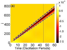
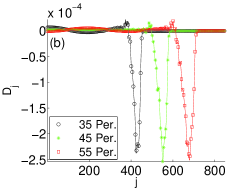
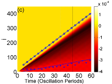
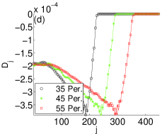
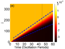
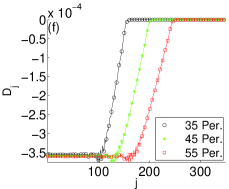
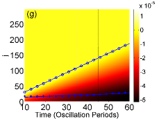
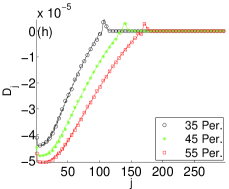
Figure 3: Spatio-temporal evolution of the asymmetry indicator ($D_{j}$, see Eq. (5)) [left panels] and its spatial dependence for particular times [right panels]. (a),(b): $\omega=10$, (c),(d): $\omega=20$; (e),(f): $\omega=30$, (g),(h): $\omega=40$. The outer-cone horizon was calculated by identifying the first value for $j$, where the wave had not yet reached and is denoted by circles. The crosses indicate the inner-cone horizon. For $\omega=\{10,20,30\}$, the location was determined by identifying the first value of $j$ to the left of the minimum of $D_{j}$ where the derivative between beads is approximately zero. For $\omega=40$, the minimum value of $D_{j}$ identifies the inner-cone horizon. To improve clarity, only every third period is shown. A linear least-squares best fit line is depicted for these locations; the slope of the line is the cone velocity. The vertical dashed lines indicate the particular times for which the spatial asymmetry profile is illustrated on the right panels. To improve clarity in the right panels, only every fifth value of $j$ is shown. The same parameters as Fig. 2 were used.

In Fig. 3, for each value of $\omega=\{10,20,30,40\}$, a contour plot illustrating the DRT profile as a function of $j$ and $t$ is provided. Additionally, the right panels show the asymmetry indicator profile of Eq. (5)) at a set of particular times, written in terms of oscillations of the center bead. A non-zero value of $D_{j}$ indicates the preferential transport of force in one direction, that is, DRT. We see that, after transient behavior, all significant values of $D_{j}$ are negative, indicating the presence of DRT towards the right hand side of the lattice (see Eq. (5)).

Figures 3(a),(b), illustrate the DRT profiles for $\omega=10$, where both $\omega$ and $2\omega$ are below $\omega_{c}$. After a transient time interval, we observe a DRT “wave”, or cone, advancing as time progresses (and leaving no DRT behind it). For this reason we call this behavior temporal DRT. For a given time, let $O$ denote the value of $j$ at the outer edge of the cone (that effectively travels at the speed of sound within the medium), $\cal{I}$ denote the value of $j$ at the inner edge of the cone, and $M$ denote the value of $j$ for which $|D_{j}|$, and therefore DRT, is maximal. For $j>O$, we have $D_{j}=0$ since the energy from the forcing function has not yet reached beads offset this far from the center bead. For the region defined by $M\leq j\leq O$, there exists a positive, approximate-linear relationship (with respect to $j$) describing the magnitude of the DRT. Similarly, for $\cal{I}$ $\leq j\leq M$, there exists a negative approximate linear relationship describing DRT magnitude. The DRT wave has already moved through the region defined by $0<j<\cal{I}$. The characteristic property of this class of behavior, which we call Class I, is that for $0<j<\cal{I}$, $D_{j}\approx 0$, indicating DRT is no longer present shortly after the wave has left a region.

Class II behavior is observed by considering a forcing frequency of 20, as shown in Figs. 3(c),(d). Here, $\omega_{c}$ is greater than $\omega$ and slightly larger than $2\omega$. After allowing for transient time, the regions defined by $j>O$, $M\leq j\leq O$, and $\cal{I}$ $\leq j\leq M$, display the same qualitative behavior as the previous case. However, what clearly distinguishes this region is that for $j<\cal{I}$ we see a qualitatively different result, namely, for each $j$, $D_{j}$ is approximately equal to a nonzero constant. This is indicative of an equilibrium DRT state defined by the spatial extent of the region through which the ratcheting wave has already passed. This effect and the “kink”-like pattern that it leads to (rather than the pulse like structure of Class I) in the context of the asymmetry indicator $D_{j}$ is hereafter referred to as spatial DRT. This fundamental distinction of regimes of temporal and spatial DRT is, arguably, one of the most interesting traits observed herein, and to our knowledge, has not been reported before, although we believe that it should be more general than the particular realization considered herein.

In Figs. 3(e),(f), $\omega$ = 30 and thus $\omega<\omega_{c}$ and $2\omega>\omega_{c}$. As a result, a different behavior that will be characterized hereafter as belonging to Class IIIA is observed. The features are similar to Class II, but now the magnitude of the spatial DRT is approximately equal to $|D_{M}|$, the maximal temporal DRT magnitude. Otherwise said, the tail of the kink associated with the asymmetric deformation of the lattice, rather than having the linear profile of Class II, it is essentially flat. As shown in Figs. 3(g),(h), where $\omega=40$, as $\omega$ approaches $\omega_{c}$, the DRT profile remains qualitatively the same, but the slope of the (approximately) linear relationship for $M\leq j\leq O$ decreases. In our kink-based visualization of the corresponding $D_{j}$’s, this regime is associated not with the translation of the structure over the lattice which roughly preserves its shape, as in Class IIIA. Instead, it appears associated predominantly with the widening of the relevant spatial structure in this regime that we will refer to as Class IIIB.

For $\omega>\omega_{c}$, neither of the plane waves comprising $u_{i^{*}}(t)$ can propagate. As a result, the spatial and temporal DRT behavior breaks down. This can be discerned in Figs. 4, and 5 where the DRT magnitude and velocity (that we will now proceed to define more precisely) approach zero as $\omega$ approaches $\omega_{c}$.

To explore the effects of parameter variation on the magnitude of the DRT, we now establish an additional ratcheting metric. For each of the DRT profiles under consideration, $D_{M}$ represents the maximal amount of temporal ratcheting at any given time. We use this value as the temporal DRT metric. On the other hand, when spatial ratcheting is present, it is first observed by comparing beads adjacent to the $i^{*}$th bead, that is at $j=1$. As time progresses, the behavior spreads out from the center bead and is also observed for larger values of $j$. We observe that $D_{j}$ is approximately the same for each $j$ exhibiting spatial DRT behavior; therefore the magnitude of spatial ratcheting can be quantified by means of $D_{1}$. Both $D_{M}$ and $D_{1}$ vary slightly over time. Nevertheless, we have verified that this variation is small and, therefore, choose to measure $D_{1}$ and $D_{M}$ at the final integration time $t_{f}$.

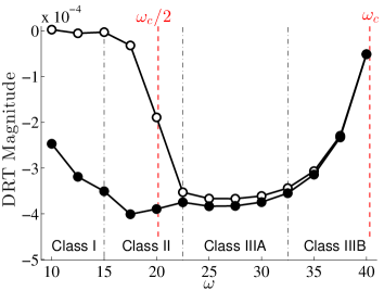
Figure 4: The magnitude of spatial and temporal DRT as a function of $\omega$. The open dots represent the magnitude of spatial DRT (as measured by $D_{1}$) while the filled dots are the magnitude of temporal DRT (as measured by $D_{M}$; see also the text). The same parameter values and conditions as Fig. 5 were used.

Figure 4 illustrates the magnitude of spatial and temporal DRT, based on the above diagnostic, for a wide range of representative frequencies. For Class I ($10<\omega<15$), the magnitude of temporal DRT slowly increases with the frequency. This regime corresponds to both input frequencies of the forcing ($\omega$ and $2\omega$) being below the cutoff frequency $\omega_{c}=40.31$. As it can be noticed in Fig. 4, the spatial DRT starts appearing once the second harmonic ($2\omega$) of the driver gets closer to the cutoff frequency (see left vertical dashed line). This seems to be an effect of the nonlinear response of the system that “widens” the region of the cutoff frequency. In fact, Class II corresponds to the region of frequencies where the second harmonic of the driver transitions from being transmitted to completely being stopped due to the cutoff frequency. It is interesting that for Class II and IIIA, defined by $15<\omega<32.5$ corresponding to $\omega<\omega_{c}$ but $2\omega$ close to (under or over) $\omega_{c}$, the temporal DRT magnitude is approximately constant. However, as the first harmonic ($\omega$) starts getting close to the cutoff frequency (see right vertical dashed line), naturally, both spatial and temporal DRT start to disappear and eventually vanish, as expected, once both, first and second, driver harmonics are inside the forbidden gap. The effect of the first harmonic starting to approach the cutoff frequency begins at, approximately, $\omega=32.5$, corresponding to the onset of Class IIIB behavior, the magnitude of temporal DRT begins to sharply decrease as $\omega$ approaches $\omega_{c}$. This lack of DRT for higher frequencies is consistent with the DRT breaking down for $\omega>\omega_{c}$. On the other hand, spatial DRT significantly increases as we move from Class I to Class II and subsequently IIIA, and it also, in turn, sharply decreases in the case of Class IIIB.

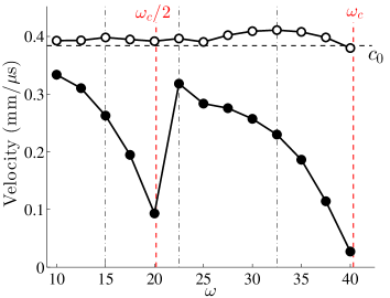
Figure 5: Outer- and inner-cone velocities as a function of $\omega$. The open dots represent the inner-cone velocities while the filled dots are the outer-cone velocities. The horizontal dotted line corresponds to the sound velocity of the system, $c_{0}$. The default parameters in Tables 1 are used with $a=\delta_{0}/100$, $\eta={4}/{9}$, and $\phi$ is averaged over 16 values. The number of center bead oscillations varies with $\omega$, but is chosen such that the associated velocity converges. $N$ and $t_{f}$ also vary with $\omega$ and are chosen such that no perturbation reaches the boundaries. The different regime classes are distinguished as indicated in the text.

We define the outer-cone horizon as the location of the onset of temporal DRT and the inner-cone horizon as the location of the onset of spatial DRT. The velocities of the outer and inner horizon are calculated numerically for values of $\omega$ ranging from 10 to 40. For each frequency, the velocity of the outer-cone horizon approximately corresponds to the sound velocity of the system, $c_{0}^{2}\equiv 6A\delta_{0}^{\frac{1}{2}}r^{2}/m$ (see filled dots in Fig. 5). This is a consequence of the nonlinearity of the system that “mixes” the frequencies introduced by the forcing and thus excites all modes. In contrast to the behavior observed by the outer-cone velocity, as shown in Fig. 5 (see open dots), the inner-cone velocity strongly depends on the forcing frequency. For small values of $\omega$, where both $\omega$ and $2\omega$ are smaller than $\omega_{c}$, there is essentially no spatial DRT, as the two cones propagate with essentially the same speed forming the “pulse” observed in the asymmetry indicator $D_{j}$. As the frequency increases through Class I and toward Class II, the velocity of the inner-cone horizon decreases significantly until the threshold $2\omega>\omega_{c}$ is crossed. At that point the inner-cone velocity approaches zero. Within Class II, the continuously decreasing velocity of the inner-cone forms the tail of the kink discussed in connection to Fig. 3. Past the point of $\omega=\omega_{c}/2$, the inner-cone velocity abruptly increases to a value similar to that for the lower frequencies. Subsequently, in Class IIIA, the velocity decreases as the case where both $\omega$ and $2\omega$ are larger than $\omega_{c}$ is approached. Class IIIB corresponds to a larger rate of decreasing velocity. Interestingly, the spatio-temporal wave velocities are independent of the choice of $\eta$.

It is interesting to point out at this stage that the presence of DRT in our system is a direct consequence of the symmetry breaking provided by the external forcing when $\eta\not=0$ [see Eq. (4)]. However, it is also important to note that nonlinearity is also a key ingredient for the presence of DRT. In fact, if the Hertzian forces in Eq. (1) are replaced by linear (Hooke) springs, DRT is no longer present. The absence of DRT for the linear force case is a consequence of the fact that the DRT corresponding to a phase $\phi$ is the negative of the one for phase $\phi+T/2$, where $T$ is the period of the driver, and thus providing a cancellation when DRT is averaged through all possible phases of the driver. Finally, it is also important to stress that, as discussed earlier and depicted in Fig. 2, the magnitude of DRT is, approximately, proportional to the cube of the forcing amplitude. Therefore, nonlinearity in the system is not only necessary for observing DRT, but it also provides a nonlinear enhancement of the DRT magnitude with respect to the input amplitude.

$\begin{array}[]{c}\includegraphics[width=156.49014pt]{Fig6a.eps}\\ \includegraphics[width=156.49014pt]{Fig6b.eps}\end{array}$

Figure 6: Magnitude of spatial and temporal DRT as a function of $\eta$. In the top panel, $\omega=17.5$ while in the bottom $\omega=30$. The open dots represent the magnitude of spatial DRT, the filled dots are the magnitude of temporal DRT, and the dashed lines correspond to the theoretical ratchet velocity function. The same parameter values and conditions as in Fig. 5 were used.

In Ref. Chacon2007 , it was shown that when considering the forcing function $u_{i^{*}}(t)$, the magnitude of DRT behavior is due to two competing effects: the increase in the degree of symmetry breaking and the decrease in the transmitted impulse over a half-period, which is denoted as effective symmetry breaking. It was shown that the DRT behavior is optimally enhanced for $\eta={2}/{3}$. We now demonstrate that this result holds for the granular crystal case under consideration. We consider forcing frequencies of $\omega$ = 17.5 and 30. Figure 6 illustrates the spatio-temporal DRT magnitude as a function of $\eta$. As is expected, for $\eta=0$, the single harmonic does not induce DRT behavior. As $\eta$ increases, the magnitude of DRT increases until a maximum value for ratcheting is reached at $\eta={2}/{3}$ (in our case since DRT is towards the left, the maximum ratcheting effect corresponds to a minimum for DRT), with the exception of spatial DRT for $\omega$ = 17.5. The magnitude then decreases until DRT is again not present at $\eta=1$. To further explore and quantitatively appreciate this result, consider a generic biharmonic forcing function $f(t)=\epsilon_{1}\sin(q\omega t+\phi_{1})+\epsilon_{2}\sin(p\omega t+\phi_{2})$, where $\epsilon_{1,2}$ are amplitudes, $\phi_{1,2}$ are phases, $\omega$ is the frequency and $p$ and $q$ are coprimes. It can be shown that the ratchet velocity $\bar{v}=\beta\left(\epsilon_{1}^{p}\epsilon_{2}^{q}\right)$ where $\beta$ is a system-dependent constant Quintero2010 . With the parameters in $u_{i^{*}}(t)$, we have $\bar{v}(\eta)=\beta\left(\eta^{2}-\eta^{3}\right)$. Observe that this function has a minimum (for $\beta<0$) at $\eta={2}/{3}$, which is consistent with the numerical simulations. By setting $\bar{v}({2}/{3})$ equal to the numerically-calculated DRT magnitude at $\eta={2}/{3}$, we can solve for the free parameter $\beta$. These curves are shown in Fig. 6. There is a striking agreement between the calculated numerical DRT magnitudes and theoretical curves. We see less of a correspondence for spatial DRT for $\omega=17.5$. In general, for other frequencies considered, the temporal DRT matched the theoretical curves more consistently than spatial DRT, particularly for $\omega$ near $\omega_{c}/2$ and $\omega_{c}$.

As a side note, it is possible to draw physical intuition for the optimal biharmonic weight being at 2/3 if one considers the ideal ratcheting forcing: a sawtooth function. Expanding a sawtooth function in Fourier series and keeping only the first two harmonics it is straightforward to show that their ratio is 2. In our case, when $\eta=2/3$, we precisely get a ratio between the two harmonics of $\eta/(1-\eta)=2$. In other words, the optimal ratcheting forcing, i.e. $\eta=2/3$, is the best possible approximation to a sawtooth function when using two harmonics.

V The Dissipative Bead-lattice

To more closely represent physical reality, dissipation is introduced into the uniform granular crystal by augmenting Eq. (1):

$$m\ddot{u}_{i}=A[\delta_{0}+u_{i-1}-u_{i}]_{+}^{\frac{3}{2}}-A[\delta_{0}+u_{i}-u_{i+1}]_{+}^{\frac{3}{2}}-\frac{m}{\tau}\dot{u}_{i},$$ (6)

where $\tau$ is a dissipation constant set equal to $1750\mu s$. This value was chosen to match the dissipation constant used in the experiments of Ref. Boechler2011 . To investigate the effects of friction, we numerically integrate the four representative frequency cases presented earlier and illustrate the corresponding results in Fig. 7. In order to allow sufficient time for transient behavior, $t_{f}$, the final integration time, and $N$ were considerably larger than for the non-friction simulations.

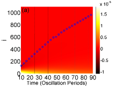
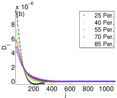
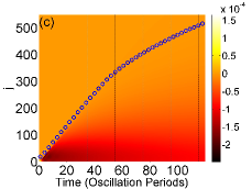
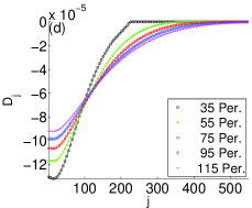
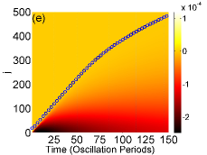
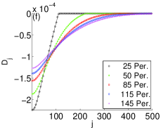
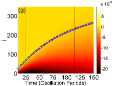
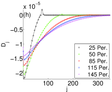
Figure 7: Asymmetry indicator contour plots and temporal cross sections in the presence of dissipation with $\tau=1750\mu s$. The layout, parameters, and conditions are identical to Fig. 3.

When friction is present, we observe that all cases exhibit qualitatively similar behavior. Namely, unlike the frictionless case, the velocity of the temporal DRT is not set by the sound velocity of the system, but instead decreases as time progresses. Furthermore, in all dissipative cases, we have observed that spatial DRT is weakened by the presence of dissipation and that all cases present a similar spatial structure which seems to involve a progressively widening (i.e., dispersing) kink state.

It is worth noticing that for $\omega=20$, the DRT profile is slightly different than for the other cases. The maximal temporal DRT value, $D_{M}$ now occurs at $M\approx 20$. Furthermore, as time increases, $D_{j}\rightarrow D_{M}$ for $j<M$. This is indicative of a small amount of spatial DRT. In fact, the behavior is similar to Class IIIB for the frictionless system. For $\omega=10$, the presence of friction radically changes the characteristics of the DRT profiles. Temporal DRT is present, but for $t\gtrsim 30$ periods, all non-zero values of $D_{j}$ are now positive, indicating that the DRT direction has reversed and now favors left propagation. For $t\lesssim 30$, the minimum of $D_{j}$ is less than zero illustrating the remnants of rightward DRT.

In each of the DRT profiles provided in Fig. 7, we observe two regimes of DRT propagation. Initially, the temporal DRT “wave” travels at the sound velocity of the system. However, as time progresses, the dissipation tend to slow down the propagation of this wave. Similarly, dissipation is also responsible for progressively damping out the DRT magnitude. Eventually, a steady state solution is reached where the energy being pumped into the system by the forcing is balanced by dissipation.

Finally, it is worth mentioning that, despite taking the optimal value for the forcing amplitude to exploit maximum DRT gain, the DRT magnitude is on the order of $10^{-5}$–$10^{-4}$ which amounts to a $10^{-3}$–$10^{-2}\%$ of biased transport between left and right propagation. Although these values are relatively small, DRT should be possible to measure in current experimental setups.

VI Conclusions

In this work, a one-dimensional granular chain (crystal) was considered where the position of the center bead was prescribed by a biharmonic forcing function. This functional form is known to induce ratcheting. Yet, in our case, a distinguishing characteristic was the system-wide emergence (i.e. in space-time) of directed ratchet transport (DRT) in the force profiles. The regimes where temporal (transient) ratcheting and spatial (i.e., with a permanent spatial “imprint” over the lattice) ratcheting were identified as a function of the system’s frequency. The relationship between the frequencies $\omega$ and $2\omega$ of the forcing function and the cutoff frequency $\omega_{c}$ of the system determined the characteristics of the observed DRT and its separation into different classes. In the class I pertaining to temporal ratcheting, a DRT “wave” traveled away from the center bead at the sound velocity of the system. Once the temporal DRT wave moved through a region, a steady-state was induced in this region, wherein all bead pairs exhibited similar DRT magnitude. If this value was non-zero, it corresponded to Class II and the so-called spatial DRT. The modification of the form of spatial ratcheting past the regime where $\omega=\omega_{c}/2$ gave rise to yet another regime that was referred to as Class III.

The frequency, $\omega$, and biharmonic weight, $\eta$ of the forcing function were varied so that the response of the magnitude of DRT and the velocity of the DRT “waves” could be determined. While the wave velocity was independent of the biharmonic weight, $\eta={2}/{3}$ maximized the magnitude of spatio-temporal DRT, in accordance with the expectations of Refs. Chacon2007 ; Quintero2010 .

Friction was subsequently introduced into the system, leading to weakening of the ratcheting effect and a rather uniform spatial form of its profile in classes II and III. Yet, it was class I that was most significantly affected by the inclusion of friction within the system, which resulted in DRT switching directionality from right to left.

Having paved the way for the consideration of ratchet effects in granular crystals, there are numerous directions along which the present study can be extended. It is certainly of interest to attempt to expand the range of considered materials and parameters (as well as that of heterogeneous systems such as dimers, trimers mason1 ; mason2 ; vakakis ) and of a wider range of forcing frequencies and displacement parameters. A key aspect of such a broader parametric effort is to try to maximize the relevant DRT, so as to render it more accessible to potential experiments. Another important direction of particular interest is to attempt to expand the present considerations to the realm of higher dimensional granular crystals. Recent efforts have made these gradually more accessible to experimental investigations andrea1 ; andrea2 and hence such ratcheting efforts would be extremely timely and relevant to consider.

- (1) L. Trujillo, F. Peniche, and X. Jia. In R. Pico Vila, editor, Waves in Fluids and Solids. InTech, 2011, Chap. V, pp. 127–152.
- (2) H.M. Jaeger, S.R. Nagel, and R.P. Behringer. Rev. Mod. Phys., 68 (1996) 1259.
- (3) S. Luding, Nature, 435 (2005) 159.
- (4) V.F. Nesterenko. Dynamics of Heterogeneous Materials. Springer-Verlag, New York, 2001.
- (5) S. Sen, J. Hong, J. Bang, E. Avalos, and R. Doney, Phys. Rep., 462 (2008) 21.
- (6) P.G. Kevrekidis, Nonlinear waves in lattices: past, present, future, IMA J. Appl. Math., 76 (2011) 389.
- (7) C. Daraio, V. F. Nesterenko, E. B. Herbold, and S. Jin, Phys. Rev. Lett., 96 (2006) 058002.
- (8) J. Hong, Phys. Rev. Lett., 94 (2005) 108001.
- (9) F. Fraternali, M. A. Porter, and C. Daraio, Mech. Adv. Mat. Struct., 17 (2010) 1.
- (10) R. Doney and S. Sen, Phys. Rev. Lett., 97 (2006) 155502.
- (11) D. Khatri, C. Daraio, and P. Rizzo, SPIE, 6934 (2008) 69340U.
- (12) A. Spadoni, C. Daraio, Proc. of the Nat. Acad. of Sci., 107 (2010) 7230.
- (13) C. Daraio, V.F. Nesterenko, E.B. Herbold, and S. Jin, Phys. Rev. E, 72 (2005) 016603.
- (14) V.F. Nesterenko, C. Daraio, E.B. Herbold, and S. Jin, Phys. Rev. Lett., 95 (2005) 158702.
- (15) N. Boechler, G. Theocharis, C. Daraio, Nature Materials, 10 (2011) 665.
- (16) P. Hänggi and F. Marchesoni, Rev. Mod. Phys., 81 (2009) 387.
- (17) M. Rietmann, R. Carretero-González, and R. Chacón. Phys. Rev. A, 83 (2011) 053617.
- (18) H.J. Carlin and Y.K. Pozhela. Proceedings of the IEEE, 53, 11 (1965) 1788.
- (19) F. Falo, P.J. Martínez, J.J. Mazo, and S. Cilla, Europhys. Lett., 45 (1999) 700.
- (20) F. Falo, P.J. Martínez, J.J. Mazo, T.P. Orlando, K. Segal, and E. Trías, Appl. Phys. A, 75 (2002) 263.
- (21) A.V. Ustinov, C. Coqui, A. Kemp, Y. Zolotaryuk, and M. Salerno. Phys. Rev. Lett., 93 (2004) 087001.
- (22) D. Poletti, T.J. Alexander, E.A. Ostrovskaya, B. Li, and Yu.S. Kivshar. Phys. Rev. Lett., 101 (2008) 150403.
- (23) M. Schiavoni, L. Sánchez-Palencia, F. Renzoni, and G. Grynberg, Phys. Rev. Lett., 90 (2003) 094101.
- (24) R. Gommers, S. Bergamini, and F. Renzoni, Phys. Rev. Lett., 95 (2005) 073003.
- (25) F. Jülicher, A. Ajdari, and J. Prost. Rev. Mod. Phys., 69 (1997) 1269.
- (26) S. Flach, O. Yevtushenko, and Y. Zolotaryuk. Phys. Rev. Lett., 84 (2000) 2358.
- (27) P. Reimann. Phys. Rep., 361 (2002) 57.
- (28) D.C. Rapaport Comp. Phys. Comm., 147 (2002) 141.
- (29) N. Boechler, G. Theocharis, S. Job, P.G. Kevrekidis, M.A. Porter, and C. Daraio. Phys. Rev. Lett., 104 (2010) 244302.
- (30) Y. Man, N. Boechler, G. Theocharis, P.G. Kevrekidis, and C. Daraio. Phys. Rev. E, 85 (2012) 037601.
- (31) N.R. Quintero, J.A. Cuesta, and R. Alvarez-Nodarse. Phys. Rev. E, 81 (2010) 030102.
- (32) L. Brillouin, Wave propagation in periodic structures; electric filters and crystal lattices, McGraw-Hill Book Company, (New York, 1946).
- (33) J. Cuevas, B. Sánchez-Rey, and M. Salerno, Phys. Rev. E, 82 (2010) 016604.
- (34) R. Chacon. J. Phys. A, 40 (2007) F413.
- (35) N. Boechler, G. Theocharis, and C. Daraio. Nature Materials, 10 (2011) 665.
- (36) M.A. Porter, C. Daraio, E.B. Herbold, I. Szelengowicz, and P.G. Kevrekidis, Phys. Rev. E, 77 (2008) 015601.
- (37) M.A. Porter, C. Daraio, I. Szelengowicz, E.B. Herbold, and P.G. Kevrekidis, Physica D, 238 (2009) (2009).
- (38) K.R. Jayaprakash, Y. Starosvetsky, and A.F. Vakakis Phys. Rev. E, 83 (2011) 036606.
- (39) A. Leonard, F. Fraternali, and C. Daraio. Experimental Mechanics, 53 (2011) 327.
- (40) A. Leonard and C. Daraio, Phys. Rev. Lett., 108 (2012) 214301.