Causal Inference in Observational Studies with Non-Binary Treatments

Abstract

Propensity score methods have become a part of the standard toolkit for applied researchers who wish to ascertain causal effects from observational data. While they were originally developed for binary treatments, several researchers have proposed generalizations of the propensity score methodology for non-binary treatment regimes. Such extensions have widened the applicability of propensity score methods and are indeed becoming increasingly popular themselves. In this article, we closely examine the two main generalizations of propensity score methods, namely, the propensity function (p-function) of Imai and van Dyk (2004) and the generalized propensity score (gps) of Hirano and Imbens (2004), along with recent extensions of the gps that aim to improve its robustness. We compare the assumptions, theoretical properties, and empirical performance of these alternative methodologies. On a theoretical level, the gps and its extensions are advantageous in that they can be used to estimate the full dose response function rather than the simple average treatment effect that is typically estimated with the p-function. Unfortunately, our analysis shows that in practice response models often used with the original gps are less flexible than those typically used with propensity score methods and are prone to misspecification. We compare new and existing methods that improve the robustness of the gps and propose methods that use the p-function to estimate the dose response function. We illustrate our findings and proposals through simulation studies, including one based on an empirical application.

Keywords: covariate adjustment, generalized propensity score, model diagnostics, propensity function, propensity score, smooth coefficient model, subclassification, nonparametric models

1 Introduction

Adjusting for observed confounding variables is one of the most common strategies used across numerous scientific disciplines when making causal infererence in observational studies. Researchers find that the results based on regression adjustments can be sensitive to model specification when applied to the data where the treatment and control groups differ substantially in terms of their pre-treatment covariates. The propensity score methods of Rosenbaum and Rubin (1983), hereafter RR, aim to address this fundamental problem by reducing the covariate imbalance between the two groups. RR showed that under the assumption of no unmeasured confounding, adjusting for propensity score, rather than potentially high-dimensional covariates, is sufficient for unbiased estimation of causal effects and this can be done by simple nonparametric methods such as matching and subclassification.

Despite their popularity, one limitation of the original propensity score methods is that they are only applicable to a binary treatment. About a decade ago, several researchers proposed generalization of the propensity score methodology for non-binary treatment regimes (Imbens, 2000; Hirano and Imbens, 2004; Imai and van Dyk, 2004). Such extensions have widened the applicability of propensity score methods and are indeed becoming increasingly popular themselves, Google Scholar citation counts of the aforementioned papers are 776, 227, and 310, respectively, as of August 8, 2013). Particularly novel applications appear in Ertefaie and Stephens (2010) and Moodie and Stephens (2012).

All of these methods, however, require users to overcome the challenges of first correctly modeling a treatment variable as a function of a possibly large number of pre-treatment covariates and second modeling the response variable. These represent significant difficulties in practice. Standard diagnostics based on the comparison of the covariate distributions between the treatment and control groups are not directly applicable to non-binary treatment regimes and the final inference can be quite sensitive to the choice of response model. Flores, Flores-Lagunes, Gonzalez, and Neumann (2012), hereafter FFGN, propose two extensions to the method of Hirano and Imbens that aim to provide more robust estimation through a move flexible response model.

In this paper, we closely examine the two main generalization of propensity score methods, namely, the propensity function (p-function) of Imai and van Dyk (2004), hereafter IvD, and the generalized propensity score (gps) of Hirano and Imbens (2004), hereafter HI, along with the FFGN extensions. We compare the assumptions and theoretical properties of these two alternative methodologies and examine their empirical performance in practice. In Section 2, we review the theoretical properties of the original propensity score methodology and its generalizations. The HI method has a theoretical advantage over the IvD method in that the former can be used to estimate the full dose response function (drf) rather than the simple average treatment effect, which is often estimated with IvD’s method. In Section 3, we compare the method of IvD, HI, and FFGN both theoretically and empirically, using a pair of simple simulation studies. We demonstrate that the response model used by HI is less flexible than those typically used with propensity score methods and that the methods proposed by FFGN to address this can exhibit undesirable properties. In Section 4, we compare these methods with a new proposal and show how the method of IvD can be extended for robust estimation of the full drf. The efficacy of the proposed methodology is illustrated through the aforementioned simulation studies in Section 4 and an empirically-based study in Section 5. Section 6 offers concluding remarks and an Appendix introduces a robust variant of HI’s method.

2 Methods

Suppose we have a simple random sample of size $n$ with each unit consisting of a $p$-dimensional column vector of pretreatment covariates, ${\bm{X}}_{i}$, the observed univariate treatment, $T_{i}$, and the outcome variable, $Y_{i}$. Although IvD’s method can be applied to multivariate treatments, here we assume the treatment is univariate to facilitate comparison with HI’s method. We omit the subscript when referring to generic values of ${\bm{X}}_{i}$, $T_{i}$, and $Y_{i}$.

We denote the potential outcomes by $\mathcal{Y}=\{Y_{i}(t),t\in\mathcal{T}$ for $i=1,\ldots,n\}$, where $\mathcal{T}$ is a set of possible treatment values and $Y_{i}(t)$ is a function that maps a particular treatment level of unit $i$, to its outcome. This setup implies the stable unit treatment value assumption (Rubin, 1990) that the potential outcome of each unit is not a function of treatment level of other units and that the same version of treatment is applied to all units. In addition, we assume strong ignorability of treamtent assignment, i.e., $Y(t)\ \mbox{$\perp\!\!\!\perp$}\ T\mid{\bm{X}}$ and $p(T=t\mid{\bm{X}})>0$ for all $t\in\mathcal{T}$, which implies no unmeasured confounding (RR).

2.1 The propensity score with a binary treatment

RR considered the case of treatment variables that take on only two values, ${\mathcal{T}}=\{0,1\}$, where $T_{i}=1$ ($T_{i}=0$) implies that unit $i$ receives (does not receive) the treatment and defined the propensity score to be the conditional probability of assignment to treatment given the observed covariates, i.e., $e({\bm{X}})=p(T=1\mid{\bm{X}})$. In practice, $e({\bm{X}})$ is typically estimated using a parametric treatment assignment model $p_{\psi}(T=1\mid{\bm{X}})$ where $\psi$ is a vector of unknown parameters. The appropriateness of the fitted model can be assessed via the celebrated balancing property of $e({\bm{X}})$, namely, that covariates should be independent of the treatment conditional on the propensity score, ${\bm{X}}\ \mbox{$\perp\!\!\!\perp$}\ T\ |\ e({\bm{X}})$. In particular, the fitted model, ${\hat{e}}({\bm{X}})=p_{\hat{\psi}}(T=1|{\bm{X}})$ should not be accepted unless adjusting for $\hat{e}({\bm{X}})$ results in adequate balance.

In order to estimate causal quantities, we must properly adjust for ${\hat{e}}({\bm{X}})$. RR propose three techniques: matching, subclassification, and covariance adjustment. Here we focus on subclassification and covariance adjustment because they are more closely related to the generalization of IvD and HI. The key advantage of propensity scores when applying these methods is the dimension reduction, requiring that we only adjust for a scalar variable ${\hat{e}}({\bm{X}})$, rather than the entire covariate vector, which is often of high dimension.

With subclassification (RR), we adjust for ${\hat{e}}({\bm{X}})$ by dividing the observations into several subclasses based on ${\hat{e}}({\bm{X}})$. Individual response models are then fitted within each subclass, adjusting for ${\hat{e}}({\bm{X}})$ and sometimes ${\bm{X}}$ along with $T$. The overall causal effect is then computed as the weighted average of the within-class coefficients of $T$, with weights proportional to the size of subclass. The standard error of the causal effect is computed typically by treating the within-subclass estimates as independent of one another.

With covariance adjustment (RR), we regress the response variable on ${\hat{e}}({\bm{X}})$ separately for the treatment and control groups. Specifically, we divide the data into the treatment and control groups and fit the regression model, ${\rm E}(Y\mid{\bm{X}},T=t)=\alpha_{t}+\beta_{t}\cdot{\hat{e}}({\bm{X}})$, seperately for $t=0,1$. The average causal effect is then estimated as

$$(\hat{\alpha}_{1}-\hat{\alpha}_{0})+(\hat{\beta}_{1}-\hat{\beta}_{0})\cdot\overline{\hat{e}({\bm{X}})}$$ (1)

where $\overline{\hat{e}({\bm{X}})}$ is the sample mean of the estimated propensity score.

In addition to the techniques in RR, inverse propensity score weighting can be used to estimate causal quantities (e.g., Rosenbaum, 1987; Robins, 1998; Robins et al., 2000; Imbens, 2000). Because the following equalities

$${\rm E}\bigg{\{}\frac{TY}{e({\bm{X}})}\bigg{\}}={\rm E}\{Y(1)\}\quad{\rm and}\quad{\rm E}\bigg{\{}\frac{(1-T)Y}{1-e({\bm{X}})}\bigg{\}}={\rm E}\{Y(0)\},$$

hold and the inverse weighting estimate,

$$\sum\limits_{i=1}^{N}\bigg{(}\ \frac{T_{i}Y_{i}}{\hat{e}({\bm{X}}_{i})}-\frac{(1-T_{i})Y_{i}}{1-\hat{e}({\bm{X}_{i}})}\ \bigg{)}$$

is an unbiased estimate of the average causal effect. Covariance adjustment and inverse weighting must be used cautiously as the scalar estimated propensity score replaces the full set of the covariates (Rubin, 2004). In particular, inverse weighting can be quite unstable in practice (see e.g., Kang and Schafer, 2007, as well as Sections 3.1 and 3.2).

Matching, subclassification, covariance adjustment, and inverse weighting all aim to provide robust flexible adjustment for $\hat{e}({\bm{X}})$ in the response model. As we shall see below, the flexibility of the response model is important especially for non-binary treatment regimes. This is because unlike the treatment assignment model which has an effective diagnostic tool based on the balancing property of propensity score, the response model lacks such diagnostics.

2.2 Generalizations of propensity score: the GPS and the P-FUNCTION

Suppose now that $\mathcal{T}$ is a more general set of treatment values, perhaps categorical or continuous. It is in this setting that IvD introduced the p-function and that HI introduced the gps (IvD also allow for multi-variate treatments, which we do not discuss in this paper). In what follows, we review and compare these generalizations of propensity score methods. In particular, we consider the following aspects of propensity score adjustment with binary treatments that both IvD and HI generalize:

1. Treatment assignment model: Model the distribution of the treatment assignment given covariates to estimate the propensity score, i.e., $\hat{e}({\bm{X}})$

2. Diagnostics: Validate ${\hat{e}}({\bm{X}})$, by checking for covariate balance, i.e., $T\mbox{$\perp\!\!\!\perp$}{\bm{X}}\mid\hat{e}({\bm{X}})$

3. Response model: Model the distribution of the response given the treatment, adjusting for ${\hat{e}}({\bm{X}})$ via matching, subclassification, covariance adjustment, or inverse weighting

4. Causal quantities of interest: Estimate the causal quantities of interest and their standard error based on the fitted response model

Treatment assignment model. As in the case of the binary treatment, we begin by modeling the distribution of the observed treatment assignment given the covariates using a parametric model, $p_{\psi}(T\mid\bm{X})$, where $\psi$ is the parameter. Common choices of $p_{\psi}(T|{\bm{X}})$ include the Gaussian or multinomial regression models when the treatment variable is continuous or categorical, respectively. HI define the gps as $R=r(T,{\bm{X}})=p_{\psi}(T\mid\bm{X})$. That is, the gps is equal to the treatment assignment model density evaluated at the observed treatment variable and covariate for a particular individual. This is analogous to the propensity score for the binary treatment, which can be written as $e({\bm{X}})=r(1,{\bm{X}})=p_{\psi}(T=1\mid{\bm{X}})$.

IvD, on the other hand, define the p-function to be the entire conditional probability density (or mass) function of the treatment, namely $e_{\psi}(\cdot\mid{\bm{X}})=p_{\psi}(\cdot\mid{\bm{X}})$. This is also analogous to the propensity score for the binary treatment case because $e_{\psi}(\cdot\mid{\bm{X}})$ is completely determined by $e({\bm{X}})=p_{\psi}(T=1\mid{\bm{X}})$. In order to summarize the p-function, IvD introduce the uniquely parameterized propensity function assumption which states that for every value of ${\bm{X}}$, there exists a unique finite-dimensional parameter, ${\bm{\theta}}\in\Theta$, such that $e_{\psi}(\cdot\mid{\bm{X}})$ depends on ${\bm{X}}$ only through ${\bm{\theta}}_{\psi}({\bm{X}})$. In other words, ${\bm{\theta}}$ uniquely represents $e\{\cdot\mid{\bm{\theta}}_{\psi}({\bm{X})\}}$, which we may therefore write as $e(\cdot|{\bm{\theta}})$ or simply ${\bm{\theta}}={\bm{\theta}}_{\psi}({\bm{X}_{i}})$. For example, if we use a normal linear model for the treatment, $T_{i}\sim{\cal N}({\bm{X}}_{i}^{\top}{\bm{\beta}},\sigma^{2})$ with $\psi=({\bm{\beta}},\sigma^{2})$, then $e_{\psi}(\cdot\mid{\bm{X}_{i}})$ is uniquely represented by the scalar ${\bm{\theta}_{i}}={\bm{X}}_{i}^{\top}{\bm{\beta}}$. In practice, $\psi$, $\bm{\theta}_{i}$, $R_{i}$, and $r_{i}$ are estimated by $\hat{\psi}$, $\bm{\hat{\theta}}_{i}$, $\hat{R}_{i}$, and $\hat{r}_{i}$

Diagnostics. Diagnostics for the treatment assignment model rely on balancing propereties of the p-function and gps. In particular, IvD shows that the p-function is a balancing score, i.e., $T\ \mbox{$\perp\!\!\!\perp$}\ \bm{X}\mid e(\cdot\mid{\bm{\theta}})$. IvD suggest checking balance by regressing each covariate on $T$ and $\hat{\bm{\theta}}$, e.g., using Gaussian and/or logistic regression and comparing the distribution of the $t$-statistics for each of the resulting regression coefficients of $T$ with the standard normal distribution via a normal quantile plot. Improvement in balance can be assessed by constructing the plot again in the same manner except that $\hat{\bm{\theta}}$ is left out of each regression. Although not typical performed, this diagnostic is equally applicable in the binary treatment case, but with $\hat{\bm{\theta}}$ replaced by $\hat{e}(\bm{X})$.

HI, on the other hand, show that $\bm{1}\{T=t\}$ is independent of ${\bm{X}}$ given $r(t,{\bm{X}})$, where $\bm{1}\{\cdot\}$ is an indicator function and the gps is evaluated at $t\in\mathcal{T}$. Following the covariate balancing property for the binary propensity score, HI construct a series of binary treatments by coarsening the original treatment $T$ in the form $\{t_{j}<T\leq t_{j+1}\}$ for some $t_{1},t_{2},\dots,t_{J}$. Covariate balance is then checked for these binary treatment variables by first subclassifying units on $\hat{r}(\widetilde{T}_{j},{\bm{X}})$, where $\widetilde{T}_{j}$ is the median of the treatment variable among units with $\bm{1}\{t_{j}<T\leq t_{j+1}\}=1$. Then, two-sample $t$-tests are performed within each subclass to compare the mean of each covariate among units with $\bm{1}\{t_{j}<T\leq t_{j+1}\}=0$ against that among units with $\bm{1}\{t_{j}<T\leq t_{j+1}\}=1$. Finally the within-subclass differences in means and the variances of these differences are combined to compute a single t-statistic for each covariate. HI suggest this diagnostics be repeated for several choices of $\{t_{1},\dots,t_{J}\}$ that cover the range of observed treatment assignment variable $T$.

In both cases, we note that the failure to reject the null hypothesis of perfect balance does not necessarily imply the lack of balance and hence these diagnostics need to be interpreted with great care. In fact, it may be the case that covariate balance is not desirable but a smaller sample size limits the ability to detect imbalance (Imai et al., 2008).

Response model. The response models proposed by IvD and HI are quite different, with HI relying more heavily on parametric assumptions. IvD propose two response models. The first is completely analogous to the subclassification technique proposed by RR. Individual response models are fitted within each subclass, adjusting for $\hat{\bm{\theta}}$ and typically ${\bm{X}}$ along with $T$. The second is a smooth coefficient model (scm), which allows the intercept and slope to vary smoothly as a function of the p-function

$$E(Y\mid T,\hat{\bm{\theta}})\ =\ f({\hat{\bm{\theta}}})+g({\hat{\bm{\theta}}})\cdot T,$$ (2)

where $f(\cdot)$ and $g(\cdot)$ are unknown but smooth continuous functions. In our numerical illustrations, we fit this model using the R package mgcv developed by Simon Wood, in which smooth functions are represented as a weighted sum of known basis functions; and the likelihood is maximized with an added smoothness penalization term. We use penalized cubic regression splines as the basis functions, with dimension equal to five.

In contrast, HI propose to estimate the conditional expectation of the response as a function of the observed treatment, $T$, and the gps, $\hat{R}$. They recommend using a flexible parametric function of the two arguments and give the following Gaussian quadratic regression model,

$$E(Y\mid T,\hat{R})\ =\ \alpha_{0}+\alpha_{1}\cdot T+\alpha_{2}\cdot T^{2}+\alpha_{3}\cdot\hat{R}+\alpha_{4}\cdot{\hat{R}}^{2}+\alpha_{5}\cdot T\cdot\hat{R}.$$ (3)

This can be viewed as a generalization of RR’s covariance adjustment technique, which in the binary treatment case involves regressing $Y$ on ${\hat{e}}({\bm{X}})$ separately for the treatment and control groups. HI, on the other hand, parametrically estimate the average outcome for all possible treatment levels simultaneously via the quadratic regression on $T$ given in (3).

Estimating causal quantities of interest. IvD and HI aim to estimate different causal quantities, IvD the average causal effect and HI the drf. Computing the average causal effect under the scm, involves averaging $g({\hat{\bm{\theta}_{i}}})$ across all units. Bootstrap standard errors are computed by resampling the data and refitting both the treatment assignment and response models. With subclassification, computing the estimated average causal effect proceeds exactly as in the binary case. Because a response model is fit conditional on $T$ within each subclass, we can in principle average these fitted models and estimate the drf. While we illustrate this possibility in our simulations, we advocate a flexible non-parametric approach in Section 4.1.

In contrast, to estimate the drf, HI computes the average potential outcome on a grid of treatment values. In particular, at treatment level $t$, they compute

$${\hat{E}}\{Y(t)\}\ =\ \frac{1}{n}\sum\limits_{i=1}^{n}\Big{(}\hat{\alpha}_{0}+\hat{\alpha}_{1}\cdot t+\hat{\alpha}_{2}\cdot t^{2}+\hat{\alpha}_{3}\cdot\hat{r}(t,{\bm{X}_{i}})+\hat{\alpha}_{4}\cdot\hat{r}(t,{\bm{X}_{i}})^{2}+\hat{\alpha}_{5}\cdot t\cdot\hat{r}(t,{\bm{X}_{i}})\Big{)}.$$ (4)

Standard errors can be calculated using the bootstrap, taking into account the estimation of both the gps and model parameters. In practice, we are often interested in the relative drf, $E\{Y(t)-Y(0)\}$, which compares the average outcome under each treatment level with that under the control, i.e., $t=0$. Of course, in some studies there is no control per se and we revert to $E\{Y(t)\}$. In our simulation studies we report the relative drf while in our applied example we report the drf which is more appropriate in its particular context.

The FFGN extensions to the method of HI. Unfortunately, the quadratic regression in (3) is less flexible than either subclassification or a scm (see Section 3.4). Bia et al. (2011) and FFGN  point out that misspecification of (3) can result in biased causal quantites and FFGN proposes two alternatives. The first generalizes (3) with,

$$E(Y\mid T,\hat{R})\ =\ \beta(T,\hat{R})$$ (5)

where $\beta(T,\hat{R})$ is a flexible nonparametric model; in our numerical studies we use a SCM. The drf, $\hat{E}\{Y(t)\}$, and its standard errors are computed as in (4), but with

$$\hat{E}\{Y(t)\}\ =\ \frac{1}{n}\sum\limits_{i=1}^{n}\hat{\beta}[t,\hat{r}(t,{\bm{X}}_{i})]$$ (6)

Because the scm is a function of the gps, we refer to this as the scm(gps) method.

The second method involves inverse weighting (iw) and estimates the drf with

$$\hat{E}\{Y(t)\}\ =\ \frac{\sum\limits_{i=1}^{N}{\tilde{K}_{h,X}}(T_{i}-t)\cdot Y_{i}}{\sum\limits_{i=1}^{N}{\tilde{K}_{h,X}}(T_{i}-t)},$$ (7)

where ${\tilde{K}_{h,X}}(T_{i}-t)=K_{h}(T_{i}-t)/\hat{r}(t,\bm{X}_{i})$, $K(\cdot)$ is a kernel function with the usual properties, $h$ is a bandwidth satisfying $h\rightarrow 0$ and $Nh\rightarrow\infty$ as $N\rightarrow\infty$, and $K_{h}(\cdot)=h^{-1}K(\cdot/h)$. This is the local constant regression (Nadaraya-Watson) estimator but now with each individual’s kernel weight being divided by its gps at $t$. To avoid boundary bias and to simplify derivative estimation, the iw approach estimates $E\{Y(t)\}$ using a local linear regression of $Y$ on $T$ with a weighted kernel function $\tilde{K}_{h,X}(T_{i}-t)$, i.e.,

$$\hat{E}\{Y(t)\}\ =\ \frac{D_{0}(t)S_{2}(t)-D_{1}(t)S_{1}(t)}{S_{0}(t)S_{2}(t)-S_{1}^{2}(t)},$$ (8)

where $S_{j}(t)=\sum\limits_{i=1}^{N}{\tilde{K}_{h,X}}(T_{i}-t)(T_{i}-t)^{j}$ and $D_{j}(t)=\sum\limits_{i=1}^{N}{\tilde{K}_{h,X}}(T_{i}-t)(T_{i}-t)^{j}Y_{i}$. The global bandwidth can be chosen following the procedure of Fan and Gijbels (1996). We use (8) as the iw estimator in our numerical studies.

3 Comparing the GPS and the P-FUNCTION

In this section, we examine the differences between the method of IvD, HI, and FFGN using both simulation studies and theoretical comparisons. The key differences lie in how each method summarizes $p(T\mid{\bm{X}})$: the gps evaluates this density at the observed covariate, whereas the p-function uniquely parameterizes it. As we show below, this difference leads to alternative choices for the response model, which can yield markedly divergent results.

3.1 Simulation study I

In our first simulation study, we have $2,000$ observations, each of which comes with a single continuous covariate, $X$, a continuous univariate treatment, $T$, and a response variable, $Y$. We simulate $X_{i}\stackrel{{\scriptstyle\rm ind}}{{\sim}}{\cal N}(0.5,0.25)$ and $T_{i}\mid X_{i}\stackrel{{\scriptstyle\rm ind}}{{\sim}}{\cal N}(X_{i},0.25)$ and assume that the potential outcome has the following distribution, $Y_{i}(t)\mid T_{i},X_{i}\stackrel{{\scriptstyle\rm ind}}{{\sim}}{\cal N}(10X_{i},1)$ for all $t\in\mathcal{T}$. In this simulation study the true treatment effect is zero and the true drf is five for all $t$. We deliberately choose this simple setting where any reasonable method should perform well. Fitting a simple linear regression of $Y$ on $T$ yields a statistically significant treatment effect estimate of roughly five. However, adjusting for $X$ in the regression model is sufficient to yield an estimate that is much closer to and is not statistically different from the true effect of zero.

Using the correctly specified treatment assignment model, $T_{i}\mid X_{i}\stackrel{{\scriptstyle\rm ind}}{{\sim}}{\cal N}(X_{i},0.25)$, we implement the HI, IvD, scm(gps), and iw methods. For the response models, we use the quadratic regression given in (3) with the method of HI, regress $Y$ on $T$ within each of $S$ subclasses with the method of IvD, and use the default models for scm(gps) and iw. For the purposes of illustration, we do not adjust for $\hat{\bm{\theta}}$ within each subclass when using IvD’s method. Owing to the linear structure of the generative model, doing so would dramatically reduce bias even with a small number of subclasses. Here we illustrate, instead, how bias can be reduced by increasing the number of subclass; we implement IvD with $S=5,10$, and $50$ subclasses. For the HI, scm(gps), and iw methods, we use a grid of ten equally spaced points between $-0.5$ and $1.5$, $t_{1},\ldots,t_{D}$ with $D=10$, to compute the relative drf and its derivative. Standard errors are computed using 1,000 bootstrap replications.

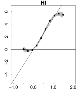
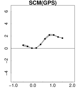
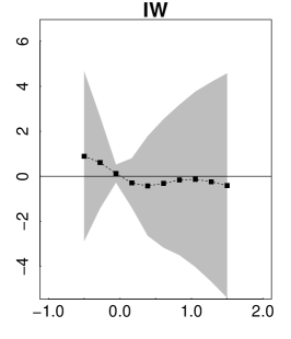
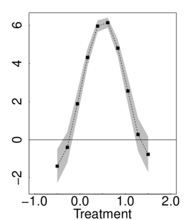
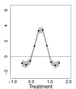
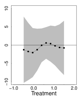
Figure 1: The Results of Simulation Study I. The first row plots the estimated relative drf where the horizontal solid black line represents the true relative drf. For IvD, we use $S=5,10,50$ subclasses. The solid black diagonal line for the method of HI is the unadjusted regression of $Y$ on $T$. The second row plots the estimated derivatives of the dose response function (drf) where the solid black line represents the truth. In both rows, the grey shaded areas represent 95% confidence intervals. The estimated derivative for iw is plotted on a different scale as its standard error is significantly larger than that of the other methods.

Figure 1 presents the results. In the first row, we plot the estimated relative drf while the second row plots the estimated derivative of the drf. For HI, scm(gps), and iw, the derivative is computed as

$${1\over 2}\left[{\hat{E}\{Y(t_{d+1})\}-\hat{E}\{Y(t_{d})\}\over t_{d+1}-t_{d}}+{\hat{E}\{Y(t_{d})\}-\hat{E}\{Y(t_{d-1})\}\over t_{d}-t_{d-1}}\right]$$ (9)

for $d=2,\ldots D-1$. For $d=1$, we simply use the first term in (9) and for $d=10$ we use the second term in (9). For IvD, the derivative is the weighted average of the within subclass linear regression coefficient; 95% point-wise confidence intervals are shaded gray.

Figure 1 shows that even in this simple simulation, all methods except IW miss the true relative drf and its derivative, albeit to differing degrees. The behavior of IvD’s estimate improves with more subclasses, a luxury we can afford here because of the large sample size. IvD makes the general recommendation that the within subclass models be adjusted for ${\bm{X}}$ or at least for $\hat{\bm{\theta}}$. Because of the simple structure of this simulation, doing so would result in a correctly specified model even with a single subclass, eliminating bias in the estimated average treatment effect. We do not recommend estimating the drf by averaging the unadjusted within subclass models, but do so here to facilitate comparisons between the methods. We propose a new estimate of the drf using the p-function in Section 4.1.

The performance of the HI method is particularly poor; It differs only slightly from the unadjusted regression. Although scm(gps) offers limited improvement, it also introduces a cyclic artifact into the fit. We will see this pattern again. The iw method, on the other hand, results in an unstable fit that is characterized by very large standard erros. The performance of these methods are especially troubling both because the gps was expressly designed to estimate the drf and because the current simulation setup is so simple. Given their performance here, it is difficult to think that these methods can succeed in more realistic settings. The primary goal of this paper is to explain why the gps-based methods can fail and to provide a more robust estimate of the drf.

One reason that gps-based methods can perform poorly is that their response model are based on overly strong parametric assumptions, especially (3). This is illustrated in Figure 2 which compares the fitted mean potential outcome as a function of the gps and $T$ under the HI model (left panel) and under scm(gps) (middle panel). The fitted potential outcomes differs substantially and are considerably more constrained under the quadratic model of HI. Although scm(gps) is more flexible than HI, it still exhibits considerable constraints. To see this we subclassified the data into 10 subclasses based on $T$, and fit a quadratic regression for $Y$ as a function of the gps seperately within each of the subclasses. Five out of the 10 within subclass fit are plotted in the right most plot in Figure 2. The results differs substantially from HI and reveals the considerable constraint of the quadratic response model. Subclassifying on $T$ in this way leads to a new response model and a corresponding new gps-based estimate of the drf; this method is discussed in Appendix A.

Figure 2: The Varying Flexibility of the Response Models. The plots show the mean potential outcome as a function of the gps and $T$ under HI’s quadratic response model (left panel), fitted scm(gps) (middle panel), and covariance adjustment gps (right panel). Covariance adjustment gps fits a quadratic regression ($Y\sim R+R^{2}$) in each of several subclasses based on $T$. See Appendix A for details. Here we use 10 subclasses; Only five are shown for ease of plotting. Judging from the plots, subclassification is by far the most flexible of the three response models.

3.2 Simulation study II

In Simulation I, although its response model is misspecified in terms of its adjustment for $X$, the IvD method may benefit from its assumption that the drf is linear in $T$. We address this in the second simulation that compares the performance of the methods under two generative models. We also explore the frequency properties of the methods.

Suppose we have a simple random sample of $2,000$ observations that consist of a univariate covariate $X$, the assigned treatment $T$, and the response $Y$, respectively. We assume that $X\stackrel{{\scriptstyle\rm ind}}{{\sim}}{\mathcal{N}}(0,1)$ and that $T$ depends on $X$ through $T\mid X\stackrel{{\scriptstyle\rm ind}}{{\sim}}{\mathcal{N}}(X+X^{2},1)$. We simulate the potential outcome $Y(t)$ using two different response models:

Linear drf:

$Y(t)\mid t,X\ \stackrel{{\scriptstyle\rm ind}}{{\sim}}\ {\cal N}(X+t,9)$

Quadratic drf:

$Y(t)\mid t,X\ \stackrel{{\scriptstyle\rm ind}}{{\sim}}\ {\cal N}((X+t)^{2},9)$

To isolate the difference between the methods, we correctly specify the treatment model for all methods. For the response model under HI and IvD’s methods, we consider Gaussian regression models that are linear and quadratic in $T$. In particular for the method of IvD we fit (i) $Y\sim T$ and (ii) $Y\sim T+T^{2}$ within each of 10 equally sized subclasses, and for the method of HI we fit (i) $Y\sim T+R+R^{2}+R\cdot T$ and (ii) $Y\sim T+T^{2}+R+R^{2}+R\cdot T$. With IvD, the relative drf is computed by averaging the coefficients of the within subclass models. The default response models are used for scm(gps) and iw. For the gps-based methods, the relative drf is evaluated at ten equally spaced values of $t$ between $-1.5$ to $5.5$. The entire procedure was repeated for all methods on each of 1000 data sets simulated from each generative model. Notice that all of the response models are misspecified in their adjustment for $X$ and/or $T$, as we expect in practice. Thus, this simulation study investigates the robustness of the methods to typical misspecification of the response model.

Generative Dose Response Function: Linear
 Generative Dose Response Function: Quadratic

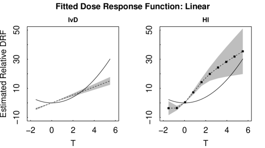
Figure 3: Estimated Relative drfs in Simulation Study II Using the Methods of IvD and HI. The solid lines plot the true relative drfs, the dashed lines plot the means of the fitted relative drfs across 1000 simulations, and the gray shaded regions correspond to two standard deviation pointwise intervals across the 1000 fitted relative drfs. The evenly-spaced grid of evaluation points used with HI are also plotted as solid circles. The method of HI shows appreciable bias with all four combinations of generative and fitted response models. The method of IvD, on the other hand, is biased only when the fitted model is of a lower order than the generative model.

Generative Dose Response Function: Linear

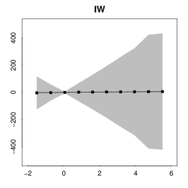
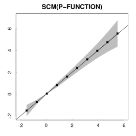
Generative Dose Response Function: Quadratic

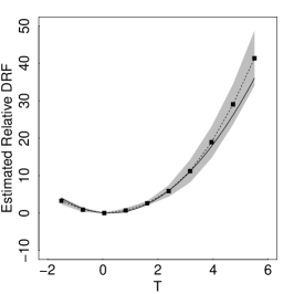
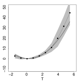
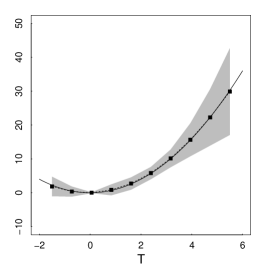
Figure 4: Estimated Relative drfs in Simulation Study II for the scm(gps), iw, and scm(p-function) Methods. Solid lines represent the true relative drf and dashed lines the average of the fitted relative drfs across 1000 simulations. Points represent the evenly-spaced grid points. Pointwise intervals containing 95% of the 1000 fitted relative drfsare shaded grey. Note that the scale of the y-axis for the iw method under linear generative drf is different from others as it has a siginificantly larger standard deviation. The scm(p-function) method is discussed in Section 4.1.

Figures 3 and 4 report the average of the estimated relative drfs across the simulations (dashed lines) along with their two standard deviation intervals (shaded regions). The true relative drf functions are plotted as solid lines. The first and second rows correspond to the true drf being linear and quadratic, respectively. The left pair of columns in Figure 3 give results when the fitted model is linear under the IvD method (column 1) and the HI method (column 2). The right pair of columns in Figure 3 give results when the fitted model is quadratic under the methods of IvD (column 3) and HI (column 4).

The IvD method performs reasonably well when the generative model is linear (row 1). In this case, the estimated drf is close to the truth. When the quadratic model is fitted (column 3), the drf is estimated with little bias though the estimate has higher variability. As shown in the lower left quadrant of the figure, the IvD method exhibits significant bias only when the true drf is of higher order (i.e., quadratic) than the fitted drf (i.e., linear). The HI method, on the other hand exhibits appreciable bias even when the response model matches the true model in its functional dependence on $t$. Like the IvD method, the bias is most acute when the fitted model is of lower order than the true model. Unlike with IvD, however, the 95% frequency intervals of HI either skirt or miss the true value completely across a wide range of treatment values.

The first two columns of Figure 4 give result for the scm(gps) and iw methods. Both methods show improvement over HI when the generative model is quadratic, although the variances are larger. For the linear generative model, scm(gps) is comparable to HI while iw exhibits enormous variance; note the change in scale of the y-axis. Using the bandwidth suggested by FFGN led to numerical instability for iw in 50 of the 1000 datasets under the linear model. Reported results are for the remaining 950 datasets.

3.3 Simulation study III

Although the scm(gps) estimate of the drf is biased in Simulation II, the cyclic bias that it exhibits in Simulation I does not appear in Figure 4. To see if the cyclic bias exists in more complex settings, we extend the well-known simulation study of Kang and Schafer (2007) to a continuous treatment. This study has a design similar to Simulation II but with a more realistic set of covariates. In particular, we independently simulate $Z_{ij}\sim N(0,1)$ for $i=1,\ldots,2000$ and $j=1,\ldots,4$. We then use the following generative models for the treatment and outcome variables,

$$T_{i}=-Z_{i1}+0.5Z_{i2}-0.25Z_{i3}-0.1Z_{i4}+\sigma_{i},$$

where $\sigma_{i}\sim N(0,1)$, and

$$Y_{i}=210+27.4Z_{i1}+13.7Z_{i2}+13.7Z_{i3}+13.7Z_{i4}+T_{i}+\epsilon_{i}$$

where $\epsilon_{i}\sim N(0,1)$. We estimate the relative drf using the methods of HI, scm(gps), and iw, on each of 1000 replicated data sets. In all cases, the treatment model is correctly specified. Figure 5 shows that the cyclic bias remains a problem for scm(gps) and that large variances continue to plague iw.

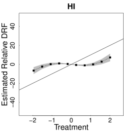
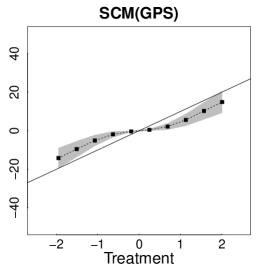
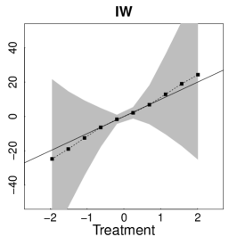
Figure 5: Estimated Relative drf in Simulation III. Solid lines, dashed lines and gray regions represent the true relative drfs  the means of the 1000 fitted relative drfs  and 95% pointwise intervals. The evaluation points are identical for all plots. scm(gps) exhibits a cyclic artifact and iw is quite unstable. The scm(p-function) method proposed in Section 4.1 again ourperforms the other methods.

3.4 Theoretical considerations and methodological implications

To understand the simulation results, we consider the tradeoff in assumptions required by the gps and p-function. In particular, while IvD make a stronger theoretical assumption of a uniquely parameterized propensity function, HI effectively make the same theoretical assumption through their choice of a parametric treatment model.

To flesh this out, we return to the observation that both the p-function and the gps can be viewed as generalizations of the p-score of RR. In the binary case, $p(T\mid{\bm{X}})$ is uniquely determined by $e({\bm{X}})=p(T=1\mid X)$. IvD focus on uniquely determining the full conditional distribution of $T$ given ${\bm{X}}$, and assume this conditional distribution is parameterized in such a way that it can be uniquely represented by $\bm{\theta}$. HI, on the other hand, do not constrain the treatment assignment model in this way and instead focus on the binary p-score as the evaluation of $p(T\mid{\bm{X}})$ at a particular value of $T$. It is important to note that the gps does not uniquely determine $p(T\mid{\bm{X}})$. There may be multiple distributions that when evaluated at a particular $T$ are equal. The assumption of a uniquely parameterized propensity function constrains the choice of treatment assignment model that can be used for a p-function. In practice, however, the same treatment assignment models are typically used by both methods.

The assumption of IvD allows a stronger form of strong ignorability of the treatment assignment given the propensity function. In particular, Result 2 of IvD states

Ignorability of IvD:

$p\{Y(t)\mid T,e(\cdot\mid{\bm{\theta}})\}=p\{Y(t)\mid e(\cdot\mid{\bm{\theta}})\}$,

Whereas, in their Theorem 2.1., HI show

Ignorability of HI:

$p_{T}\{t\mid r(t,{\bm{X}}),Y(t)\}=p_{T}\{t\mid r(t,{\bm{X}})\}$ for every $t$.

In the case where $T$ is categorical, HI’s ignorablity implies that $\mathbf{1}\{T=t\}$ and $Y(t)$ are independent given $r(t,{\bm{X}})$, where the gps is evaluated at the particular value of $t$ in the indicator function. Although achieving conditional independence of $Y(t)$ and $T$ would require conditioning on a family of gps, HI provide an insightful moment calculation to show how the response model described in Section 2.2 can be used to compute the drf. Nonetheless conditioning on either $R$ or $r(t,{\bm{X}})$, for any particular value of $t$ does not guarantee that $T$ will be uncorrelated with the potential outcomes. This restricts the response models that can be used. Subclassification, for example, is not feasible unless the classifying variable is low dimensional. The advantage of IvD is that independence between $Y(t)$ and $T$ is achieved by conditioning on a low-dimensional p-function, as parameterized by ${\bm{\theta}}$, enabling the use of a wide-range of response models.

3.5 Simulation study IV: The potential cyclic bias of SCM(GPS)

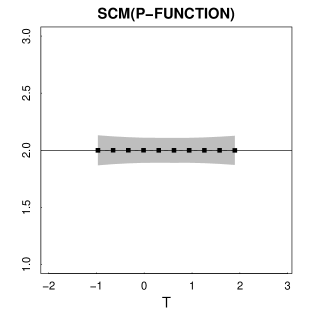
Figure 6: Estimated DRF for Simulation IV. The left plot correspond to the scm(gps) method and the right plot to a new method, scm(p-function), that is introduced in Section 4. Solid lines, dashed lines and gray regions represent the true relative drfs  the means of the 1000 fitted relative drfs  and 95% pointwise intervals. The evaluation points are identical for both plots. The scm(p-function) method does not exhibit the cyclic bias of scm(gps).

The drf fitted with scm(gps) in Simulations I and III exhibits a cyclic artifact that does not exist in the underlying drf. Here we present a simulation study that investigates the origin of this cyclic bias. In particular, we independently generate $Z_{i}\sim\rm{Bernoulli}(0.5)$, $X_{i}\sim{\cal N}(Z_{i},0.01)$, $T_{i}\sim{\cal N}(X_{i},1)$, and $Y_{i}\sim{\cal N}(4Z_{i},1)$, for $i=1,\ldots,2000$. Using the correct treatment model, we estimate the drf using scm(gps) at ten evenly spaced theoretical percentiles of $T$. We repeat the entire fitting procedure on each of 1000 replicated data sets and plot the average of the estimated drf and their pointwise two standard deviation intervals in Figure 6. The cyclic bias of the fit is evident.

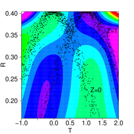
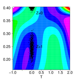
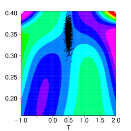
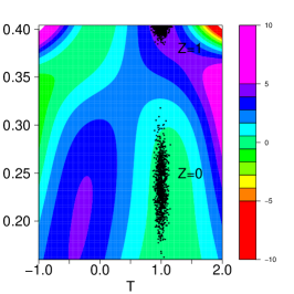
Figure 7: The scatter plot of $T$ and gps on top of the heat map of the fitted response model in Simulation IV. Left most column plots the scatter plot of ($T$,$R$). The rest three columns plots the scatter plot of ($t_{i}$,$r(t_{i},{\bm{X}}_{i}$) ), with $t_{i}$ equal to 0, 0.5, and 1. (We generate some random noise in the $T$ direction for ease of plotting.) The heat map is based on the fitted response model $\hat{f}(T,R)$.

To see the source of the cyclic bias, we plot the fitted response model given in (5) as a heat map in the leftmost panel of Figure 14. The two bell-shaped curves that appear in the plotted values of ($T_{i},\hat{R}_{i}$) stem from the definition of the gps – it is the value of the fitted density function of $T$. By the simulation design, $X$ clusters around the two values of $Z$; these two clusters correspond to the two bell-shaped curves. Generally speaking, the overlapping bell-shaped curves induce a cyclic patter in the fitted response model. To estimate the drf at $t$, the fitted response model is evaluated and averaged over each $\hat{r}(t,{\bm{X}}_{i})$. As $t$ increases, the cyclic patter in the fitted response model leads to a corresponding pattern in the fitted DRF (see Figure 6).

The patterned behavior of the gps means that the response model is particularly difficult to accurately represent, even with a flexible non-parametric model. The resulting complexity of the response model means that extrapolation is especially dangerous. Unfortunately, this is inevitable: when estimating the DRF we must evaluate the fitted response model at each value of $\hat{r}(t,{\bm{X}}_{i})$, including at unobserved combinations of $t$ and ${\bm{X}}_{i}$, see (5) and (6). This is a difficulty with the underlying response model, regardless of the choice of fitted response model. Although Simulation IV uses a simple setting to clearly explain the cyclic bias of scm(gps), problems persist in more complex settings (see Figures 1, 5, and 10).

4 Estimating the DRF Using the P-FUNCTION

In this section, we propose a new method for robust estimation of the drf using the p-function. Appendix A discusses another new robust gps-based method.

4.1 Using the P-FUNCTION in a SCM to estimate the DRF

IvD developed the p-function to estimate the average treatment effect, rather than the full drf. Nonetheless we use the framework of IvD to compute the drf in Simulation studies I and II (see Figures 1 and 3). The method we employ, however, is constrained by its dependence on the parametric form of the within subclass model. Practitioners would generally prefer a robust and flexible drf, and here we propose a procedure that allows such estimation. We view this estimate as the best available for non-binary treatments in an observational study.

We begin by writing the drf as

$$E[Y(t)]=\int E[Y(t)\mid{\bm{\theta}}]\ p({\bm{\theta}})d{\bm{\theta}}=\int E[Y(T)\mid{\bm{\theta}},T=t]\ p({\bm{\theta}})d{\bm{\theta}}$$ (10)

where the first equality follows from the law of iterated expectation and the second from the strong ignorability of the treatment assignment given the p-function. We estimate the drf using the right-most expression in (10) which we flexibly model using a scm,

$$E[Y(T)\mid{\bm{\theta}},T=t]\ =\ f({\bm{\theta}},T),$$ (11)

where $f(\cdot)$ is a smooth function of ${\bm{\theta}}$ and $T$. In practice we replace $\bm{\theta}$ by $\hat{\bm{\theta}}$ from the fitted treatment model. We approximate the integral in (10) by averaging over the empirical distribution of $\hat{\bm{\theta}}$, to obtain an estimate of the drf using a scm of the p-function,

$$\hat{E}[Y(t)]\ =\ {1\over n}\sum^{n}_{i=1}\hat{f}({\hat{\bm{\theta}_{i}}},t),$$ (12)

where $\hat{f}(\cdot)$ is the fitted scm. We refer to this method of estimating the drf as the scm(p-function) method and typically evaluate (12) on a grid of values of $t_{1},\ldots,t_{D}$ evenly spaced in range of the observed treatments, as suggested by HI. Bootstrap standard errors are computed on the same grid.

Comparing (5)–(6) with (11)–(12), scm(gps) and scm(p-function) are algorithmically very similar. The primary difference is the choice between the p-function and gps in the response model. As we shall see, this change has a siginificant effect on the statistical properties of the estimates. Simpy put, ${\bm{\theta}}$ is a much better behaved predictor variable than is $R$. When using Gaussian linear regression for the treatment model, for example, $\bm{\theta}={\bm{X}}_{i}^{\top}\beta$, whereas $R$ is the Gaussian density evaluated at $T$. As illustrated in Section 3.5, the dependence of the gps on $t$ and the non-monotonicity of this dependence both complicate the response model and pose challenges to robust estimation.

Computing $\hat{E}[Y(t_{0})]$ with (12) for some particular $t_{0}$ involves evaluating $\hat{f}(\cdot,t_{0})$ at every observed value of $\hat{\theta}_{i}$. Invariably, the range of $\hat{\theta}$ observed among units with $T$ near $t_{0}$ is smaller than the total range of $\hat{\theta}$, at least for some values of $t_{0}$. Thus, evaluating (12) involves some degree of extrapolation, at least for some values of $t$. Luckily, this problem is relatively easy to diagnose with a scatter plot of the observed values of $(T_{i},\hat{\theta}_{i})$. The estimate in (12) may be biased for values of the treatment where the range of observed $\hat{\theta}_{i}$ is relatively small. As we illustrate in our simulation studies, however, (12) appears quite robust and this bias is small relative to the biases of other available methods.

4.2 Simulation studies I–IV revisited

We now revisit the simulation studies from Section 3, which illustrate the potentially misleading results or high variance of existing gps-based methods. Here, we compare these results with those of scm(p-function). In all cases, scm(p-function) was fitted using the same (correct) treatment assignment model and with the same equally-spaced grid points. When fitting the scm, we continue to use the penalized cubic regression spline basis for both parameters ($R$ and $T$) and a tensor product to construct a smooth fit of the continuous function $f(\theta,T)$ (see mgcv R-package documentation). Figure 8 and the right panel of Figure 6 show the fitted (relative) drf for scm(p-function) in Simulations I and IV, respectively. The performance of scm(p-function) is a dramatic improvement over that of the gps-based methods (see Figures 1 and 6).

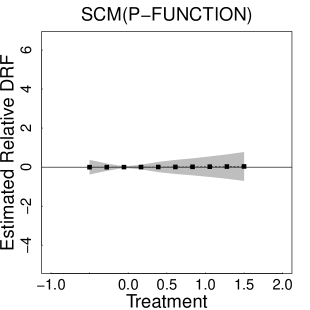
Figure 8: Estimated Relative DRF Using the scm(p-function) Method in Simulation Study I. The solid (dashed) lines represent the true (fitted) relative drf, the 95% confidence bands are plotted in grey, and the grid points are identical to those in Figure 1. The fitted relative drfs are much improved compared with those of HI, scm(gps), and iw but without the linear assumptions of IvD (see Figure 1).

Figure 4 presents the results of the scm(p-function) method in Simulation study II. Comparing Figure 4 with Figure 3 again illustrates the advantages of the proposed method. The fits in Figure 3 are quite dependent on the parametric choice of the response model, whereas the non-parametric fits illustrated in Figure 4 do not require a parametric form. Among the non-parametric methods, the advantage of scm(p-function) is clear. It essentially eliminates bias with only a small increase in variance in this simulation.

Finally, the rightmost panel of Figure 5 shows that scm(p-function) performs very well in Simulation III with no noticable bias and small variance. Overall, scm(p-function) appears to provide more robust estimates of a drf in an observational study than do any other available methods.

5 Example: The effect of smoking on medical expenditures

5.1 Background

We now illustrate our proposed methods by estimating the drf of smoking on annual medical expenditures. The data we use were extracted from the 1987 National Medical Expenditure Survey (NMES) by Johnson et al. (2003). Its detailed information about frequency and duration of smoking allows us to continuously distinguish among smokers and estimate the effects of smoking as a function of how much they smoke. The response variable, medical costs, is verified by multiple interviews and additional data from clinicians and hospitals. IvD used the propensity function to estimate the average effect of smoking on medical expenditures. We extend their analysis and study estimation of the full drf. Like IvD, we adjust for the following subject-level covariates: age at the times of the survey, age when the individual started smoking, gender, race (white, black, other), marriage status (married, widowed, divorced, separated, never married), educational level (college graduate, some college, high school graduate, other), census region (Northeast, Midwest, South, West), poverty status (poor, near poor, low income, middle income, high income), and seat belt usage (rarely, sometimes, always/almost always).

To measure the cumulative exposure to smoking based on the self-reported smoking frequency and duration, Johnson et al. (2003) proposed using the variable of packyear, which is defined as

$${\tt packyear}=\frac{\rm{number~{}of~{}cigarettes~{}per~{}day}}{20}\times\rm{number~{}of~{}years~{}smoked}.$$ (13)

We use ${\rm log}({\tt packyear})$ as our treatment variable. We follow Johnson et al. (2003) and IvD and discard all individuals with missing values and conduct a complete-case analysis, yielding a sample of 9,073 smokers. Although in general complete-case propensity-score-based analyses produce biased causal inference unless the data are missing completely at random (D’Agostino and Rubin, 2000), Johnson et al. (2003) showed that accounting for the missing data using multiple imputation did not significantly affect their results.

Because the observed response variable, self-reported medical expenditure, denoted $Y$, is semicontinuous, we use the two-part model of Duan et al. (1983). This involves first modeling the probability of spending some money on medical care, ${\rm Pr}(Y>0\mid T,\bm{X})$, where $T={\rm log}({\tt packyear})$, and $\bm{X}$ represents the covariates; and then modeling the conditional distribution of $Y$ given $T$ and $\bm{X}$ for those who reported positive medical expenditure. To illustrate and compare methods for computing the drf, we concentrate on the second part of this model. Because the distribution of $Y$ is skewed, we consider the model $p({\rm log}(Y)\mid Y>0,T,{\bm{X}})$.

For our treatment assignment model, we use a Gaussian linear regression adjusted for all available covariates and the second order terms of two age covariates. The model was fitted using sampling weights provided with the original data. This is the same treatment assignment model used by IvD who demonstrate that it achieves adequate balance.

5.2 Simulation study based on the smoking data

Figure 9: Diagnostic for the scm(p-function) method. Because the range of the $\hat{\theta}_{i}$ when $T_{i}>3$ is less than the overall range of $\hat{\theta}_{i}$ estimating the drf for $t>3$ involves extrapolation under the scm and thus possible bias. The single individual with $T_{i}$ slightly larger than three and $\hat{\theta}_{i}$ less than one is circled. To a certain extent this datapoint should mitigate bias for $t$ near three. Nonetheless, the fitted drf for $t>3$ may be seriously biased.

This simulation study aims to mimic the characteristics of the actual data with the goal of comparing the statistical properties of the proposed methods in as realistic a setting as possible. In particular, we do not alter the observed covariates or treatment and use the same fitted treatment model used by IvD. Figure 9 presents a scatter plot of the observed treatment variable, $T_{i}=\log({\tt packyear})$, and the values of the p-function from the fitted treatment assignment model, $\hat{\theta}_{i}$. As discussed in Section 4.1, this plot can be used as a diagnostic for scm(p-function). Recall that this estimate requires that we fit a scm to predict the response variable as a function of $T_{i}$ and $\hat{\theta}_{i}$. To estimate the drf at $t$ we must evaluated the fitted scm at $(t,\hat{\theta}_{i})$ using each observed $\hat{\theta}_{i}$ in the data set. This involves extrapolation and thus possible bias if the range of $\theta_{i}$ at a particular value of $t$ is less than the overall range of $\theta_{i}$. Judging from Figure 9, this is a concern for $t$ greater than about three. There is a solitary individual with $T_{i}$ slightly above three and $\hat{\theta}_{1}<1$ that is circled in Figure 9. Even this single point can guard against significant extrapolation bias for $t$ less than three, but the concern remains for $t$ in the range of 4 to 5. We emphasize that this diagnostic is preformed before the response model is fit.

To explore the robustness of the methods to different drfs, we simulate the response variable under three known drfs and attempt to reconstruct them using the HI, scm(gps), iw, covariance adjustment gps, and scm(p-function) methods. In particular, we assume $\log(Y_{i}(t))\sim{\cal N}({\rm E}[\log(Y_{i}(t))],0.5^{2})$ where $t=\log({\tt packyear})$ and consider three functional forms for ${\rm E}[\log(Y_{i}(t))]$:

$${\rm Quadratic\ DRF:} E[\log(Y_{i}(t))]\ =\ \frac{4}{25}\cdot t^{2}+[\log({\tt age}_{i})]^{2}$$

$${\rm Piecewise-Linear\ DRF:} E[\log(Y_{i}(t))]\ =\ \begin{cases}-4-0.5\cdot t+[\log({\tt age}_{i})]^{2},&t\leq 2\cr-5-2.3\cdot(t-2)+[\log({\tt age}_{i})]^{2},&t>2,\end{cases}$$

$${\rm Hockey-Stick\ DRF:} E[\log(Y_{i}(t))]\ =\ \begin{cases}-8.1+[\log({\tt age}_{i})]^{2},&t\leq 3\cr-8.1+1.5\cdot(t-3)^{2}+[\log({\tt age}_{i})]^{2},&t>3,\end{cases}$$

where age is the age at the time of the survey. We include age because it is the covariate most correlated with $\log({\tt packyear})$ and thus most able to bias a naive analysis. Each of the response models was fitted using the sampling weights.

Each of the four methods was fitted to one data set generated under each of the three drfs. We evaluate the drf at ten points equally spaced between the 5% and 95% quantiles of ${\rm log}({\tt packyear})$. The results appear in Figure 10 where rows correspond to the three generative models and columns represent the method used to fit the drf. In all plots, the true drf is plotted as a solid line and a directly fitted scm of ${\rm log}(Y)$ on $T$ as a dashed line. This scm fit is a simple bench mark; it does not account for covariates in any way, in particular it does not adjust for any summary of the treatment assignment model. Dotted lines represent the fitted drf using each of the four methods; bullets indicate the grid where the estimates are evaluated. The shaded regions around the fits represent 95% point-wise bootstrap confidence intervals. The diagnostic described in Figure 9 indicates possible bias in the scm(p-function) method for $t>3$. Thus, we plot the fit in this region in light grey to emphasize its potential unreliability.

The fit under the HI method misses the true drf under all three generative models, even the quadratic drf which coincides with the parametric dependence of ${\rm log}(Y)$ on $T$ under HI’s response model. Instead, HI’s fitted drf tends to follow the unadjusted scm fit of ${\rm log}(Y)$ on $T$. Although scm(gps) exhibits improvement over the HI method, it still exhibits a cyclic pattern; notice its cubic-like fits in the first and third rows. Unfortunately, iw again exhibits instability, although in this case it takes the form of bias rather than variance. Finally, scm(p-function) closely matches the true drf under all three generative models, at least for $t<3$. As discussed above, we suspect bias for $t>3$ and see that the fitted drf reverts to the unadjusted scm in this range. The quality of the fit can be improved still further by increasing the dimension of the basis used in the scm. We do not purse this strategy, however, for fear of over fitting. Overall, the scm(p-function) estimate appears to be the most reliable, especially considering the diagnostic that alerts us the ranges of $t$ where there is the potential for bias.

Generative Model: Quadratic

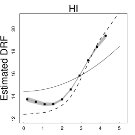
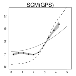
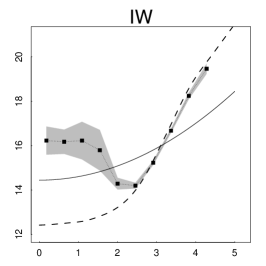
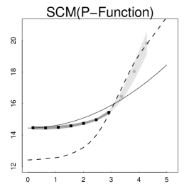
Generative Model: Piecewise Linear

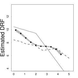
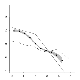
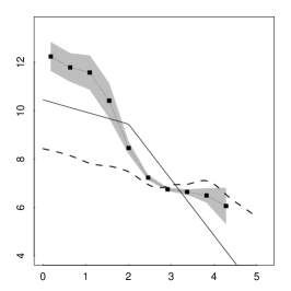
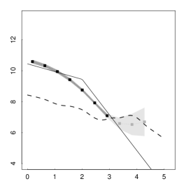
Generative Model: Hockey-stick

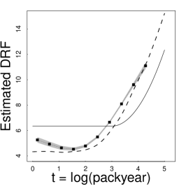
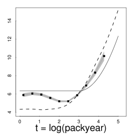
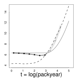
Figure 10: Estimated drfs for the Simulation Based on Smoking Data. The four columns correspond to the method of HI, scm(gps), iw, and scm(p-function) respectively. In all plots the dotted lines with bullets correspond to the fitted drf. The true drf is plotted as solid lines while dashed lines represent the fitted scm of $\log(Y)$ on $T$, unadjusted for the covariates. The evaluation points are evenly-spaced in $t$. The 95% asymptotic confidence bands plotted in grey are based on 1000 bootstrap replications. A lighter shade of grey is used in the right-most column for $t>3$ because the estimate is less reliable in this region. The performance of the scm(p-function) clearly dominates the other methods, especially for $t<3$.

6 Concluding Remarks

Propensity score methods have gained wide popularity among applied researchers in a number of disciplines. Although propensity score methods were originally designed exclusively for binary treatment regimes, the fact that treatment variables of interest are not binary in many scientific research settings has led to recent proposals for generalized propensity score methods. These methods are applicable to a variety of non-binary treatment regimes, and their applications are becoming increasingly common.

In this article, we identify and address limitations of the two most frquently used generalized propensity score methods, the gps of Hirano and Imbens (2004) and p-function of Imai and van Dyk (2004), as well as the two gps-based methods of FFGN. First, we show that the suggested implementation of the HI method is sensitive to misspecification of the response model. Second, we show that while scm(gps) exhibits substantial improvement over HI’s method, it remains biased and/or can exhibit a cyclic artifact in some situations. Third, while the IvD method provides a relatively robust method for average causal effect, its main limitation is its inability to estimate the drf. We show how to obtain an estimate of the drf based on the p-function and empirically compare its performance to that of the gps-based estimates. We also give an explanation as to why the scm(p-function) method outperforms the scm(gps) method.

There are several important challenges that must still be addressed. We have assumed throughout the paper that the gps and p-function can be correctly estimated. This is an optimistic assumption given that modeling a multi-valued or continuous treatment in a high-dimensional covariate space is much more difficult than doing so for a binary treatment (see e.g., Imai and Ratkovic, 2013, for a method that addresses this issue). Diagnostic tools developed for the binary treatment case are also not directly applicable to general treatment regimes. Even more challenging is diagnosing misspecification in the response model. As we have illustrated, this can lead to significant bias in the estimated drf. Our proposals rely on implementing more flexible response models in more natural spaces, but principled diagnostics for the response model remain elusive. Diagnosing and correcting for inbalance in either the p-function or the gps is another difficulty. Since the subpopulation that has propensity for treatment varies with the dose, the estimated dose response function is in effect the treatment effect on a varying subpopulation. Future research must develop methods for estimating the gps and p-function in the presence of possible misspecification of the treatment assignment model and the drf in the presence of possible misspecification of the response model, as well as diagnostics for both models.

ONLINE SUPPLEMENTAL MATERIALS

Appendix A Appendix: Covariance Adjustment GPS

A.1 Covariance adjustment for catagorical treatments

One of the response models suggested by RR for a binary treatment in an observational study involves covariance adjustment. With this method, the response variable is regressed on the fitted p-score separately for the treatment and control groups. Suppose we use the gps in place of the p-score in the context of a binary treatment. Specifically, for units in the treatment group, we use the ordinary p-score, $R_{i}=r(1,{\mathbf{X}}_{i})=p_{\psi}(T=1\mid{\mathbf{X}}_{i})$, but for units assigned to the control group, we use the probability of control rather than the probability of treatment, $R_{i}=r(0,{\mathbf{X}}_{i})=p_{\psi}(T=0\mid{\mathbf{X}}_{i})$. Because the gps is equal to the p-score for treatment units and is equal to one minus the p-score for control units (Imbens, 2000), it is easy to see that the usual covariance adjustment is equivalent to fitting the following regression model,

$$Y_{i}\ \sim\ \alpha_{t}+\beta_{t}\hat{R}_{i},$$ (14)

separately for the treatment and control units, i.e., $t=0$ and $1$. The linear transformation of the predictor variable does not effect the predicted value of the response for the control group.

After fitting the model given in equation (14), the average of the two potential outcomes can be estimated by averaging the fitted values over all units in the sample. That is, we compute

$$\hat{E}\{Y(t)\}\ =\ {1\over n}\sum_{i=1}^{n}\left\{\hat{\alpha}_{t}+\hat{\beta}_{t}\ \hat{r}(t,{\mathbf{X}}_{i})\right\},$$ (15)

for $t=0,1$. The estimated average causal effect is simply the difference $\hat{E}\{Y(1)\}-\hat{E}\{Y(0)\}$, which is equivalent to the estimate reported in equation (1). Thus, with a binary treatment, the method of HI is equivalent to RR’s covariate adjustment, except that HI propose a quadratic rather than a linear response model.

Suppose now that the treatment variable is categorical with more than two levels. In principle, exactly the same procedure can be applied. Namely, the regression model given in equation (14) can be fitted separately for units in each treatment group and the average potential outcome can be computed using the formula of equation (15) for each level of the treatment. We refer to this procedure as covariate adjustment gps for categorical treatments. The relative drf can be estimated as $\hat{E}\{Y(t)\}-\hat{E}\{Y(0)\}$ for each level of $t$. The validity of this procedure follows directly from the theory of RR because we only consider two treatments at a time.

If the categorical treatment variable is ordinal with a meaningful numerical scale, we can use the quadratic regression model of equation (3) suggested by HI. However, such a model is restrictive because the slope for gps in the model changes in a particular way across the treatment levels. Figure 2 shows that this assumption may be too strong to justify in practice.

The usefulness of the covariance adjustment gps for categorical variables is limited by our ability to fit multiple regression models with limited data. When the treatment takes a large number of values, the method may be infeasible. This problem is even more acute for continuous treatments where it is simply impossible to fit a separate regression model for each observed treatment level. We now discuss the covariate adjustment for continuous treatments.

A.2 Covariance adjustment GPS for continuous treatments

To use covariance adjustment with a continuous treatment variable, we propose to subclassify the data on the treatment variable rather than on the gps or the p-function. To facilitate the computation of standard errors via bootstrap (see below), we form the subclasses using the theoretical quantiles of the fitted treatment assignment model. This is typically easy to accomplish via Monte Carlo. We draw a large sample from the fitted treatment assignment model with parameters fixed at their fitted values and covariates sampled from their observed values and estimate the theoretical quantiles based on this sample. We also compute the theoretical median, or its Monte Carlo approximation, within each subclass and denote it as $t_{s}$ for $s=1,\dots,S$ with $S$ the number of subclasses.

With the subclassifed data in hand, we fit the model defined in equation (14) separately for each subclass. Alternatively, we can use a more flexible model. Here, we consider both quadratic regression, i.e., $Y_{i}\sim\alpha_{t}+\beta_{t}\hat{R}_{i}+\gamma_{t}\hat{R}_{i}^{2}$, and the scm given in equation (2) with $T$ replaced by $\hat{R}$. We then compute the gps for each unit at the median treatment value within each subclass, i.e., $\hat{r}(t_{s},{\mathbf{X}}_{i})$ for $i=1,\ldots,n$ and $s=1,\ldots,S$. Finally, we estimate the drf by computing $\hat{E}\{Y(t_{s})\}$ for each $t_{s}$ using equation (15) or an appropriate generalization of it if a different response model is used. The derivative of the drf at $t_{s}$ can be estimated as in (9). Notice that the grid values at which we compute the drf are different than those advocated by HI. Ours are based on percentiles of the fitted treatment assignment model, whereas theirs are equally spaced in the range of observed treatments.

The standard bias-variance tradeoff arises when selecting the number of subclasses, $S$. We generally defer to Cochran’s advice and use about five (Cochran, 1968). Sensitivity to the choice of $S$ can be quantified by repeating the entire procedure with $S$ equal to approximately three and ten. One source of bias in this procedure results from using units with a range of treatment values to fit the model given in equation (14) (or a more flexible version of it). This bias will be especially acute in subclasses with a relatively wide range of the treatment value. If the distribution of the treatment has tails in either direction this correspond to extreme evaluation points of the drf, $t_{1}$ and $t_{S}$. Thus, in some cases, we might want to increase the number of subclasses, especially when the extremities of the drf are of interest. This point is illustrated in Sections A.3.

We approximate the standard errors of the estimated drf and its estimated derivative via bootstrap resampling. We resample the data, fit the treatment model, subclassify, and compute the drf and its derivative for each resampled data as described above. We use the same evaluation points, $t_{1},\ldots,t_{S}$ for each resampled data set. Because both the treatment assignment model and the response model are fitted to each bootstrap sample, this procedure accounts for both sources of uncertainty.

A.3 The numerical performance of Covariance Adjustment GPS

We now examine the performance of covariance adjustment gps in Simulations I and II, as well as in the estimation of the drf of smoking on annual medical expenditures. In Simulation I, we again use the the correct treatment assignment model, $S=10$ subclasses with grid points at the $5\%,15\%,\ldots,$ and $95\%$ quantiles of $T$, (Using $S=5$ or 15 gives similar results.), and three within subclass response models: (i) $Y\sim R$, (ii) $Y\sim R+R^{2}$, and (iii) $Y\sim f(R)$, where $f(\cdot)$ is a scm. The results are shown in Figure 11. The three response models are labelled linear, quadratic, and SCM fit within subclasses, respectively. The response models are conditional on $R$, rather than on $T$ as in Section 3.1 because covariance adjustment gps subclassifies on $T$. As mentioned in Section A.2, the fitted relative drf exhibit bias in extreme subclasses owing to the relatively large range of treatment levels in these classes. Because the three within subclass models used with covariance adjustment gps lead to very similar fits, we only present results for the quadratic model in the rest of this article.

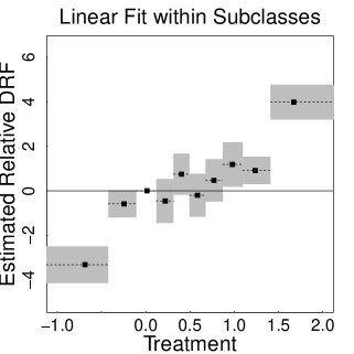
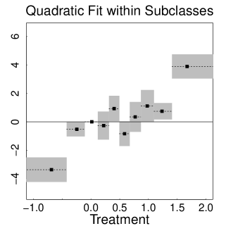
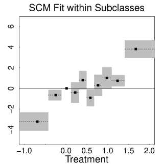
Figure 11: Estimated Relative drfs in Simulation Study I for the Covariance Adjustment gps Method. The three plots correspond to the three within subclass models. In all plots the solid (dashed) lines represent the true (fitted) relative drf and 95% confidence bands based on 1000 bootstrap replications are plotted in grey.

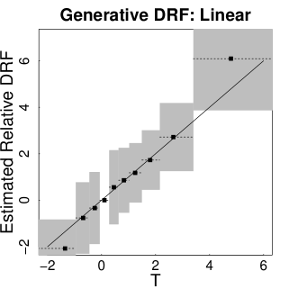
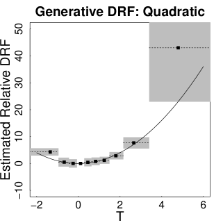
Figure 12: Estimated Relative drfs in Simulation Study II for the Covariance Adjustment gps Method. Solid lines represent the true relative drf and dashed lines the average of the fitted relative drfs across 1000 simulations. Points represent the theoretical quantiles of $T$ used to construct the subclasses. The grey shaded regions represent pointwise intervals containing 95% of the 1000 fitted relative drfs. Except in the extreme subclasses, the estimated drf appears to be essentially unbiased.

In simulation II, we use the correct treatment assignment model and a quadratic model within each of $S=10$ subclasses as the response model. (Using $S=7$ or 13 and/or the other two within subclass models yields similar results.) Results are shown in Figure 12. Except in the two most extreme subclasses, the estimated drf appears to be essentially unbiased. As in Simulation study I, the fitted relative drf deteriorates in the extreme, more heterogeneous treatment subclasses. Because the distribution of treatment is right skewed, this is less of a problem for the left-most than for the right-most subclass. This along with the blocky nature of the fitted drf may lead many users to prefer the smooth fitted relative drf obtained with scm(p-function).

Figure 13 shows the estimated drf for the simulation based on the applied-example in Section 5. We used $S=7,10,$ and $13$ subclasses using linear, quadratic, and SCM fits of $\log(Y)$ on $\hat{R}$ within each subclass. The results are all similar and we only present those with $S=10$ using a quadratic model within subclass fit. For this fit, the drf is evaluated at the midpoint of each subclass, corresponding to the theoretical 5%, 15%, …, 95% quantiles of $\log({\tt packyear})$. The covariance adjustment gps method exhibits a marked improvement over the HI method, especially for subclasses that do not contain the extreme values of $t$. The general shape of the estimated drfs is very similar to those estimated with scm(gps), see Figure 10.

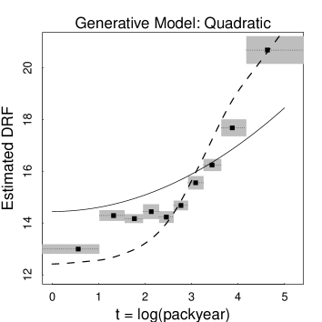
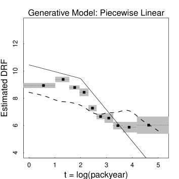
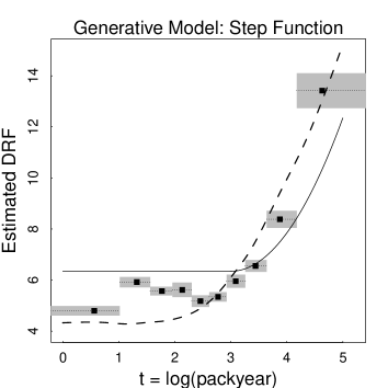
Figure 13: Estimated drf for the Simulation Based on Smoking Data Using the Covariance Adjustment gps Method. The three columns correspond to the quadratic, piecewise linear, and step function generative model. In all plots the dotted lines with bullets correspond to the fitted drf. The true drf is plotted as solid lines while dashed lines represent the fitted scm of $\log(Y)$ on $T$, unadjusted for the covariates. Evaluation points are based on the theoretical quantiles of $\log({\tt packyear})$. The 95% asymptotic confidence bands plotted in grey are based on 1000 bootstrap replications.

References

- Bia et al. (2011) Bia, M., Flores, A. C., and Mattei, A. (2011). Nonparametric estimators of dose-response functions. CEPS/INSTEAD .
- Cochran (1968) Cochran, W. G. (1968). The effectiveness of adjustment by subclassification in removing bias in observational studies. Biometrics 24, 295–313.
- D’Agostino and Rubin (2000) D’Agostino, Ralph B., J. and Rubin, D. B. (2000). Estimating and using propensity scores with partially missing data. Journal of the American Statistical Association 95, 451, 749–759.
- Duan et al. (1983) Duan, N., Manning, W. G., Morris, C. N., and Newhouse, J. P. (1983). A comparison of alternative models for the demand for medical care. Journal of Business & Economics Statistics 1, 2, 115–126.
- Ertefaie and Stephens (2010) Ertefaie, A. and Stephens, D. A. (2010). Comparing approaches to causal inference for longitudinal data: Inverse probability weighting versus propensity scores. The International Journal of Biostatistics 6.
- Fan and Gijbels (1996) Fan, J. and Gijbels, I. (1996). Local Polynomial Modelling and its Applications. Chapman and Hall, London.
- Flores et al. (2012) Flores, C. A., Flores-Lagunes, A., Gonzalez, A., and Neumann, T. C. (2012). Estimating the effects of length of exposure to instruction in a training program: The case of job corps. The Review of Economics and Statistics 94, 1, 153–171.
- Hirano and Imbens (2004) Hirano, K. and Imbens, G. W. (2004). The propensity score with continuous treatments. In Applied Bayesian Modeling and Causal Inference from Incomplete-Data Perspectives: An Essential Journey with Donald Rubin’s Statistical Family, chap. 7. Wiley.
- Imai et al. (2008) Imai, K., King, G., and Stuart, E. A. (2008). Misunderstandings among experimentalists and observationalists about causal inference. Journal of the Royal Statistical Society, Series A (Statistics in Society) 171, 2, 481–502.
- Imai and Ratkovic (2013) Imai, K. and Ratkovic, M. (2013). Covariate balancing propensity score. Journal of the Royal Statistical Society, Series B (Statistical Methodology) Forthcoming.
- Imai and van Dyk (2004) Imai, K. and van Dyk, D. A. (2004). Casual inference with general treatment regimes: Generalizing the propensity score. Journal of the American Statistical Association 99, 854–866.
- Imbens (2000) Imbens, G. W. (2000). The role of the propensity score in estimating dose-response functions. Biometrika 87, 3, 706–710.
- Johnson et al. (2003) Johnson, E., Dominici, F., Griswold, M., and Zeger, S. L. (2003). Disease cases and their medical costs attributable to smoking: An analysis of the national medical expenditure survey. Journal of Econometrics 112, 135–151.
- Kang and Schafer (2007) Kang, J. D. Y. and Schafer, J. L. (2007). Demystifying double robustness: A comparison of alternative strategies for estimating a population mean from incomplete data. Statistical Science 22, 4, 523–539.
- Moodie and Stephens (2012) Moodie, E. E. and Stephens, D. A. (2012). Estimation of dose-response functions for longitudinal data using the generalised propensity score. Statistical Methods in Medical Research 21, 2, 149–166.
- Robins (1998) Robins, J. M. (1998). Marginal structural models. 1997 Proceedings of the American Statistical Association, Section on Bayesian Statistical Science 1–10.
- Robins et al. (2000) Robins, J. M., Hernn, M. A., and Brumback, B. (2000). Marginal structural models and causal inference in epidemiology. Epidemiology 11, 550–560.
- Rosenbaum (1987) Rosenbaum, P. R. (1987). Model-based direct adjustment. Journal of the American Statistical Association 82, 398, 387–394.
- Rosenbaum and Rubin (1983) Rosenbaum, P. R. and Rubin, D. B. (1983). The central role of the propensity score in observational studies for causal effects. Biometrika 70, 41–55.
- Rubin (1990) Rubin, D. B. (1990). Comments on “on the application of probability theory to agricultural experiments. essay on principles. section 9,” by j. splawa-neyman, translated from the polish and edited by d. m. dabrowska and t. p. speed. Statistical Science 5, 472–480.
- Rubin (2004) Rubin, D. B. (2004). On principles for modeling propensity scores in medical research. Pharmacoepidemiology And Drug Safety 13, 855–857.