An Expectation-Maximization Algorithm for the Matrix Normal Distribution

Abstract.

Dramatic increases in the size and dimensionality of many recent data sets make crucial the need for sophisticated methods that can exploit inherent structure and handle missing values. In this article we derive an expectation-maximization (EM) algorithm for the matrix normal distribution, a distribution well-suited for naturally structured data such as spatio-temporal data. We review previously established maximum likelihood matrix normal estimates, and then consider the situation involving missing data. We apply our EM method in a simulation study exploring errors across different dimensions and proportions of missing data. We compare these errors and computational running times to those from two alternative methods. Finally, we implement the proposed EM method on a satellite image dataset to investigate land-cover classification separability.

1. Introduction

Technological advances in recent decades have ushered in a new era in data management and analysis. The dimension of data sets continues to grow alongside the number of observations. Consequently, the estimation of parameters or characteristics of these data remains a significant challenge. Specifically, the covariance matrix of such high dimensional data can be extremely difficult to estimate and handle. An increasingly common simplification is the assumption that this covariance has a kronecker product structure.

Not only does this structure ease the estimation procedure, it naturally fits many situations in a more physical way. Multivariate repeated measures data, for example, provides this type of framework (Boik, 1991; Naik and Rao, 2001; Roy and Khattree, 2005; Roy A., 2005). That is, the response variables and time are two separate dimensions of the data that can be characterized independently. Thus, a straightforward way to model the full covariance is via the kronecker product of a covariance of the responses and a covariance of time.

Similarly, multivariate time series of other types such as longitudinal data (Chaganty and Naik, 2002; Galecki, 1994) and spatio-temporal data (Shitan and Brockwell, 1995; Fuentes, 2004) lend themselves to this kind of covariance decomposition. To this end, classic work has been done on estimates for the matrix normal distribution:

(1) $$X\sim MN(\mu,\Sigma_{s},\Sigma_{c}),$$

where $X$ and $\mu$ are $p\times q$ matrices, $\Sigma_{s}$ is a $p\times p$ matrix and $\Sigma_{c}$ is a $q\times q$ matrix (Dawid, 1981; Dutilleul, 1999; Srivastava and Khatri, 1979; Srivastava et al, 2008). The matrix normal distribution is synonymous with this kronecker covariance structure since if $X$ has the above matrix normal distribution, then

$${\mbox{\rm vec}}(X)\sim N({\mbox{\rm vec}}(\mu),\Sigma_{c}\otimes\Sigma_{s}),$$

where $\Sigma_{c}\otimes\Sigma_{s}$ denotes the kronecker product of $\Sigma_{c}$ and $\Sigma_{s}$ and ${\mbox{\rm vec}}(X_{i})$ denotes the vectorization of $X_{i}$. While maximum likelihood estimates have been derived along with tests of whether a covariance matrix has this structure, the issue of missing data in this context has not been addressed. In this article we derive an expectation-maximization (EM) algorithm (Dempster et al, 1977) for estimating the parameters of the matrix normal distribution when missing data exists. With expressions for the estimates in hand, we conduct a simulation study and apply the method to remotely sensed data collected from the Moderate Resolution Imaging Spectroradiometer (MODIS) sensor aboard the AQUA and TERRA satellite platforms (Friedl et al, 2009).

2. Methods

We begin with $N$ independent observations from a matrix normal distribution,

$$X_{i}\stackrel{{\scriptstyle\text{\tiny iid}}}{{\sim}}MN(\mu,\Sigma_{s},\Sigma_{c}),\quad i=1,\dots,N,$$

where $X_{i}$ and $\mu$ are $p\times q$ matrices, $\Sigma_{s}$ is $p\times p$ and $\Sigma_{c}$ is $q\times q$. The use of this structure reduces the number of parameters by explicitly describing the covariance between the rows and the covariance between the columns as opposed to an individual covariance in each cell of the upper triangle of the full, $pq\times pq$, covariance matrix. Besides this simplification, the partitioning of the covariance follows naturally from a setup involving two physical, or separable, dimensions such as space and time.

2.1. Parameter Estimation with Complete Data

It is straightforward to estimate the parameters of a matrix normal distribution using maximum likelihood when there is no missing data. If $X_{i}\stackrel{{\scriptstyle\text{\tiny iid}}}{{\sim}}MN(\mu,\Sigma_{s},\Sigma_{c})$ then, equivalently,

$${\mbox{\rm vec}}(X_{i})\stackrel{{\scriptstyle\text{\tiny iid}}}{{\sim}}N({\mbox{\rm vec}}(\mu),\Sigma_{c}\otimes\Sigma_{s})$$

and so

$${\mathbb{P}}(X_{i};\mu,\Sigma_{c},\Sigma_{s})=(2\pi)^{-\frac{pq}{2}}|(\Sigma_{c}\otimes\Sigma_{s})^{-1}|^{\frac{1}{2}}\\ \exp\Bigg{\{}-\frac{1}{2}{\mbox{\rm vec}}(X_{i}-\mu)^{\top}(\Sigma_{c}\otimes\Sigma_{s})^{-1}{\mbox{\rm vec}}(X_{i}-\mu)\Bigg{\}}.$$

As usual in multivariate normal densities, in the exponential term we have the Mahalanobis distance $D_{\Sigma}(X_{i},\mu)$, with $\Sigma:=\Sigma_{c}\otimes\Sigma_{s}$, between $X_{i}$ and $\mu$,

$$D_{\Sigma}(X_{i},\mu)\doteq{\mbox{\rm vec}}(X_{i}-\mu)^{\top}(\Sigma_{c}\otimes\Sigma_{s})^{-1}{\mbox{\rm vec}}(X_{i}-\mu).$$

This distance can be worked through known identities of the vec operator and kronecker product to yield a simpler expression for the matrix normal density:

$$\begin{split}D_{\Sigma}(X_{i},\mu)&={\mbox{\rm vec}}(X_{i}-\mu)^{\top}(\Sigma_{c}\otimes\Sigma_{s})^{-1}{\mbox{\rm vec}}(X_{i}-\mu)\\ &\stackrel{{\scriptstyle\text{\tiny(i)}}}{{=}}{\mbox{\rm vec}}(X_{i}-\mu)^{\top}(\Sigma_{c}^{-1}\otimes\Sigma_{s}^{-1}){\mbox{\rm vec}}(X_{i}-\mu)\\ &\stackrel{{\scriptstyle\text{\tiny(ii)}}}{{=}}{\mbox{\rm vec}}(X_{i}-\mu)^{\top}{\mbox{\rm vec}}[\Sigma_{s}^{-1}(X_{i}-\mu)\Sigma_{c}^{-1}]\\ &\stackrel{{\scriptstyle\text{\tiny(iii)}}}{{=}}{\mbox{\rm tr}}\Big{[}(X_{i}-\mu)^{\top}\Sigma_{s}^{-1}(X_{i}-\mu)\Sigma_{c}^{-1}\Big{]}\\ &={\mbox{\rm tr}}\Big{[}\Sigma_{c}^{-1}(X_{i}-\mu)\Sigma_{s}^{-1}(X_{i}-\mu)^{\top}\Big{]}\end{split}$$

where (i), (ii), and (iii) are applications of identities (488), (496), and (497) in (Petersen and Pedersen, 2008), respectively. Furthermore, since

$$|(\Sigma_{c}\otimes\Sigma_{s})^{-1}|=|\Sigma_{c}^{-1}|^{p}|\Sigma_{s}^{-1}|^{q}$$

by identity (492) in (Petersen and Pedersen, 2008), we recover the characterization of Srivastava and Khatri (1979): $X_{i}\sim MN(\mu,\Sigma_{s},\Sigma_{c})$ if and only if the density of $X_{i}$ is given by

(2) $${\mathbb{P}}(X_{i};\mu,\Sigma_{c},\Sigma_{s})=(2\pi)^{-\frac{pq}{2}}|\Sigma_{s}|^{-\frac{q}{2}}|\Sigma_{c}|^{-\frac{p}{2}}\\ \exp\Bigg{\{}-\frac{1}{2}{\mbox{\rm tr}}\Big{\{}\Sigma_{c}^{-1}(X_{i}-\mu)\Sigma_{s}^{-1}(X_{i}-\mu)^{\top}\Big{\}}\Bigg{\}}.$$

The log likelihood of the parameters $\Theta=(\mu,\Sigma_{s},\Sigma_{c})$ is then

(3) $$\log{\mathbb{P}}(X_{1},\ldots,X_{n};\Theta)=\sum_{i}\log{\mathbb{P}}(X_{i};\Theta)\\ \qquad=\frac{pN}{2}\log|\Sigma_{c}^{-1}|+\frac{qN}{2}\log|\Sigma_{s}^{-1}|-\frac{N}{2}\log\sigma^{2}\\ -\frac{1}{2\sigma^{2}}\sum_{i}D_{\Sigma}(X_{i},\mu)$$

up to a normalizing constant. The form in (2) simplifies the matrix derivatives of (3) considerably leaving us with the following maximum likelihood estimates (MLEs):

(4) $$\begin{split}\widehat{\mu}&=\frac{1}{N}\sum_{i=1}^{N}X_{i}\\ \widehat{\Sigma}_{c}&=\frac{1}{pN}\sum_{i=1}^{N}(X_{i}-\widehat{\mu})^{\top}\widehat{\Sigma}_{s}^{-1}(X_{i}-\widehat{\mu})\\ \widehat{\Sigma}_{s}&=\frac{1}{qN}\sum_{i=1}^{N}(X_{i}-\widehat{\mu})\widehat{\Sigma}_{c}^{-1}(X_{i}-\widehat{\mu})^{\top}\end{split}$$

The two covariance estimates depend on each other and thus their estimates must be computed in an iterative fashion until convergence.

Handling non-identifiability

If for any $\kappa\neq 0$ we define $\tilde{\Sigma}_{c}:=\kappa\Sigma_{c}$ and $\tilde{\Sigma}_{s}:=\Sigma_{s}/\kappa$ then $\tilde{\Sigma}_{c}\otimes\tilde{\Sigma}_{s}=\Sigma_{c}\otimes\Sigma_{s}$, and so both estimates yield the same overall covariance matrix. To resolve this non-identifiability issue we propose the following amendment to the model:

(5) $${\mbox{\rm vec}}(X_{i})\sim N({\mbox{\rm vec}}(\mu),\sigma^{2}\Sigma_{c}\otimes\Sigma_{s})$$

and require that $(\Sigma_{c})_{11}=1$ and $(\Sigma_{s})_{11}=1$ (the choice of the top-left entry is arbitrary.) In this way we fix the scale of $\Sigma_{c}$ and $\Sigma_{s}$, and estimate the scale of the overall covariance in $\sigma^{2}$.

The MLE of $\sigma^{2}$ is

$$\widehat{\sigma}^{2}=\frac{1}{pqN}\sum_{i=1}^{N}(X_{i}-\widehat{\mu})^{\top}(\widehat{\Sigma}_{c}\otimes\widehat{\Sigma}_{s})^{-1}(X_{i}-\widehat{\mu})$$

and depends on the other estimates. The MLE for $\mu$ is clearly the same as in (4) since we only changed the variance of the model. However, since the variance scale is now captured by $\sigma^{2}$ we need to scale the MLEs for $\Sigma_{c}$ and $\Sigma_{s}$ by their top-left entry at each iteration: if $\widehat{\Sigma}^{*}_{c}$ and $\widehat{\Sigma}^{*}_{s}$ are the estimates from (4) for $\Sigma_{c}$ and $\Sigma_{s}$, then the respective MLEs for (5) are $\widehat{\Sigma}_{c}=\widehat{\Sigma}^{*}_{c}/(\widehat{\Sigma}^{*}_{c})_{11}$ and $\widehat{\Sigma}_{s}=\widehat{\Sigma}^{*}_{s}/(\widehat{\Sigma}^{*}_{s})_{11}$.

Finally, we remark that, according to Srivastava et al (2008, Theorem 3.1), if $N>\max(p,q)$ then the maximum likelihood estimates are unique.

2.2. Parameter Estimation with Missing Data

Missing data presents a difficult, albeit well-studied challenge in parameter estimation. Traditional methods, such as the EM algorithm, can usually handle missing data in a straightforward way. As the dimensionality increases, as in our case, the method can become quite computationally expensive. Naturally, we aim to assess different ways of achieving accurate parameter estimates with an eye towards reducing computation time.

The first approach (which we label “$MM$”) applies a maximization in two ways: 1) “imputation” of missing values and 2) maximum likelihood parameter estimation. In particular, the missing values get replaced by the most recent estimate of the mean. The next iteration of mean and covariance estimates come from the same maximum likelihood expressions in (4), with the addition of $\widehat{\sigma}^{2}$, based on the fully imputed data. The ease and simplicity of this method make it a natural first step in handling missing data, but also hinder its robustness and ability to capture all of the uncertainty associated with missing data.

The second approach (“$GEM$”) applies the EM algorithm to the most general version of the model. As opposed to estimating the parameters of (5), the EM algorithm provides parameter estimates for the following model:

(6) $${\mbox{\rm vec}}(X_{i})\sim N({\mbox{\rm vec}}(\mu),\Sigma).$$

These multivariate normal EM estimates have the same form of those found in McLachlan and Krishnan (1997). This approach does not simplify the original problem since it requires more parameters to be estimated by not assuming the kronecker structure. The simple form of (6) attracts much attention, but its complexity far exceeds that of (5). Where sources of variation in the data can be naturally partitioned, such as in space or time, the kronecker structure surpasses (6) in both interpretability and computational efficiency. The remainder of this article explains an EM procedure for (5) and its superiority in situations involving these types of structured data.

EM Algorithm for Matrix Normal Distribution

In the situation where missing data exists the EM algorithm is a convenient way to estimate the parameters $\Theta=(\mu,\Sigma_{c},\Sigma_{s},\sigma^{2})$ in (5). The rest of this section details the third approach (“$EM$”) to parameter estimation with missing data. Let us denote $X=(Y,Z)$ where $Z$ is the missing portion of $X$ and $Y$ is the observed portion of $X$. For the E-step, we need:

$$Q(\Theta;\Theta^{(t)})\doteq{\mathbb{E}}_{Z{\,|\,}Y;\Theta^{(t)}}[\log{\mathbb{P}}(X_{1},\ldots,X_{n};\Theta)]\\ \qquad=\frac{pN}{2}\log|\Sigma_{c}^{-1}|+\frac{qN}{2}\log|\Sigma_{s}^{-1}|-\frac{N}{2}\log\sigma^{2}\\ -\frac{1}{2\sigma^{2}}\sum_{i}{\mathbb{E}}_{Z{\,|\,}Y;\Theta^{(t)}}[D_{\Sigma}(X_{i},\mu)],$$

while the M-step updates $\Theta$ by maximizing $Q$,

$$\Theta^{(t+1)}\doteq\mathop{\rm arg\,max}\limits_{\Theta}Q(\Theta;\Theta^{(t)}),$$

via matrix differentiation in our case.

The Mahalanobis distance obeys a Pythagorean relationship: if $\tilde{\mu}_{i}^{(t)}:={\mathbb{E}}_{Z{\,|\,}Y;\Theta^{(t)}}[X_{i}]$, then

$${\mathbb{E}}_{Z{\,|\,}Y;\Theta^{(t)}}[D_{\Sigma}(X_{i},\mu)]={\mathbb{E}}_{Z{\,|\,}Y;\Theta^{(t)}}[D_{\Sigma}(X_{i},\mu_{i}^{(t)})]+D_{\Sigma}(\mu_{i}^{(t)},\mu).$$

From here the update for $\mu$ follows from $\partial Q/\partial\mu=0$:

$$\widehat{\mu}^{(t+1)}=\frac{1}{N}\sum_{i=1}^{N}\tilde{\mu}_{i}^{(t)},$$

similarly to the plain MLE case in (4).

Updating $\Sigma_{c}$, $\Sigma_{s}$ and $\sigma^{2}$ requires a bit more work. To this end we focus, first, on the following term:

$$R_{i}(\Theta;\Theta^{(t)})\doteq{\mathbb{E}}_{Z{\,|\,}Y;\Theta^{(t)}}[D_{\Sigma}(X_{i},\mu_{i}^{(t)})]\\ ={\mathbb{E}}\Big{[}{\mbox{\rm tr}}[(\Sigma_{c}\otimes\Sigma_{s})^{-1}{\mbox{\rm vec}}(X_{i}-\tilde{\mu}_{i}^{(t)}){\mbox{\rm vec}}(X_{i}-\tilde{\mu}_{i}^{(t)})^{\top}]\Big{]}\\ ={\mbox{\rm tr}}\Big{[}(\Sigma^{-1}_{c}\otimes\Sigma^{-1}_{s})\underbrace{{\mathbb{E}}[{\mbox{\rm vec}}(X_{i}-\tilde{\mu}^{(t)}_{i}){\mbox{\rm vec}}(X_{i}-\tilde{\mu}^{(t)}_{i})^{\top}]}_{V_{i}^{(t)}}\Big{]}.$$

where we define the expected outer product

$$V_{i}^{(t)}\doteq{\mathbb{E}}_{Z{\,|\,}Y;\Theta^{(t)}}[{\mbox{\rm vec}}(X_{i}-\tilde{\mu}^{(t)}_{i}){\mbox{\rm vec}}(X_{i}-\tilde{\mu}^{(t)}_{i})^{\top}].$$

To get the partial derivatives of $Q$ with respect to $\Sigma_{c}$ we need

$$\begin{split}\frac{\partial R_{i}}{\partial(\Sigma_{c}^{-1})_{kl}}&={\mbox{\rm tr}}\left\{\frac{\partial}{\partial(\Sigma_{c}^{-1})_{kl}}[(\Sigma_{c}^{-1}\otimes\Sigma_{s}^{-1})V_{i}]\right\}\\ &={\mbox{\rm tr}}\left\{\left(\underbrace{\frac{\partial\Sigma_{c}^{-1}}{\partial(\Sigma_{c}^{-1})_{kl}}}_{S_{kl}}\otimes\Sigma_{s}^{-1}\right)V_{i}\right\}\end{split}$$

where $S_{kl}$ is the structure matrix (Petersen and Pedersen, 2008) of a symmetric matrix, that is, $S_{kl}=[\delta_{ik}\cdot\delta_{jl}+\delta_{il}\cdot\delta_{jk}]_{ij}$. Thus, $(S_{kl}\otimes\Sigma_{s}^{-1})$ is a block matrix.

We can now look at $V_{i}$ as a $q\times q$ block matrix where each element is a $p\times p$ matrix in the following way, for example:

(7) $$\hskip 57.81621pt\begin{matrix}&b&\\ V_{i,kl}=&\begin{bmatrix}\circ&\circ&\circ&\circ&\circ&\circ&\circ\\ \circ&\bullet&\circ&\bullet&\circ&\bullet&\circ\\ \circ&\circ&\circ&\circ&\circ&\circ&\circ\\ \circ&\bullet&\circ&\bullet&\circ&\bullet&\circ\\ \circ&\circ&\circ&\circ&\circ&\circ&\circ\end{bmatrix}&\begin{matrix}\\ b^{\prime}\\ \\ \\ \\ \end{matrix}\end{matrix}$$

So the matrix $V_{i}$ being a block matrix leads to $V_{i,kl}$ being a symmetric $p\times p$ matrix with zeros at the empty circles in (7) and ${\mbox{\rm Cov}}_{Z_{i}{\,|\,}Y_{i}}(Z_{kb},Z_{lb^{\prime}})$ at the filled circles. Thus,

$$\frac{\partial R_{i}}{\partial(\Sigma_{c}^{-1})_{kl}}={\mbox{\rm tr}}[\Sigma_{s}^{-1}(V_{i,kl}+V_{i,kl}^{\top})]\\ =\sum_{b,b^{\prime}\in\text{\sf miss}(k,l)}(\Sigma_{s}^{-1})_{b,b^{\prime}}{\mbox{\rm Cov}}_{Z_{i}{\,|\,}Y_{i},\Theta^{(t)}}[Z_{kb},Z_{lb^{\prime}}].$$

Here miss$(k,l)$ are the row-column pairs for which there are missing entries in $V_{i}$, and $V_{i,kl}$ is the $p\times p$ block submatrix of $V_{i}$ from rows $(k-1)p+1$ to $kp$ and columns $(l-1)p+1$ to $lp$. Note that $\partial R_{i}/\partial(\Sigma_{c}^{-1})_{k,l}$ does not depend on $Z_{i}$. Moreover, the conditional covariances in ${\mbox{\rm Var}}_{Z_{i}{\,|\,}Y_{i},\Theta^{(t)}}[Z_{i}]$ above can be obtained by applying the SWEEP operator (Goodnight, 1979) to the rows of $\Sigma_{c}^{-1}\otimes\Sigma_{s}^{-1}$ that correspond to missing values.

Thus, from solving $\partial Q/\partial(\Sigma_{c}^{-1})=0$, we have

(8) $$\widehat{\Sigma}_{c}^{(t+1)}=\frac{1}{\widehat{\sigma}^{2^{(t)}}pN}\sum_{i}\Bigg{(}\frac{\partial R_{i}}{\partial\Sigma_{c}^{-1}}+(\tilde{\mu}^{(t)}_{i}-\mu^{(t)})^{\top}\Sigma_{s}^{-1^{(t)}}(\tilde{\mu}^{(t)}_{i}-\mu^{(t)})\Bigg{)}.$$

Similarly, for $\widehat{\Sigma}_{s}$,

(9) $$\widehat{\Sigma}_{s}^{(t+1)}=\frac{1}{\widehat{\sigma}^{2^{(t)}}qN}\sum_{i}\Bigg{(}\frac{\partial R_{i}}{\partial\Sigma_{s}^{-1}}\\ +(\tilde{\mu}^{(t)}_{i}-\mu^{(t)})\Sigma_{c}^{-1^{(t)}}(\tilde{\mu}^{(t)}_{i}-\mu^{(t)})^{\top}\Bigg{)}.$$

Finally, for $\sigma^{2}$,

(10) $$\widehat{\sigma}^{2^{(t+1)}}=\frac{1}{pqN}\sum_{i}R_{i}\\ +{\mbox{\rm vec}}(\tilde{\mu}^{(t)}_{i}-\widehat{\mu}^{(t)})^{\top}(\widehat{\Sigma}^{(t)}_{c}\otimes\widehat{\Sigma}^{(t)}_{s})^{-1}{\mbox{\rm vec}}(\tilde{\mu}^{(t)}_{i}-\widehat{\mu}^{(t)}).$$

Just as in the last section, we normalize these covariance estimates by their upper-left entry; i.e. $(\widehat{\Sigma}_{c})_{11}$ and $(\widehat{\Sigma}_{s})_{11}$. Detailed information regarding the implementation of this EM method can be found in the Appendix, with R code included in the supplementary material.

3. Case Studies

3.1. Simulation Study

To empirically assess the model and algorithm we simulated data from a matrix normal distribution with randomly chosen parameters of dimensions: $p=3$ and $q=5$, and $p=3$ and $q=7$. Three sample sizes were used: 250, 500, and 1000. Four different proportions of missing data were used: 5%, 10%, 15% and 20%. Data was simulated 100 times at each combination of sample size and proportion of missing data to evaluate how the accuracy of the estimates vary. The three different algorithms described in Section 2.2 were run in each of these combinations to provide a richer comparison. In order to compare these methods, the covariance errors were always measured with respect to the full (kronecker product) covariance matrix.

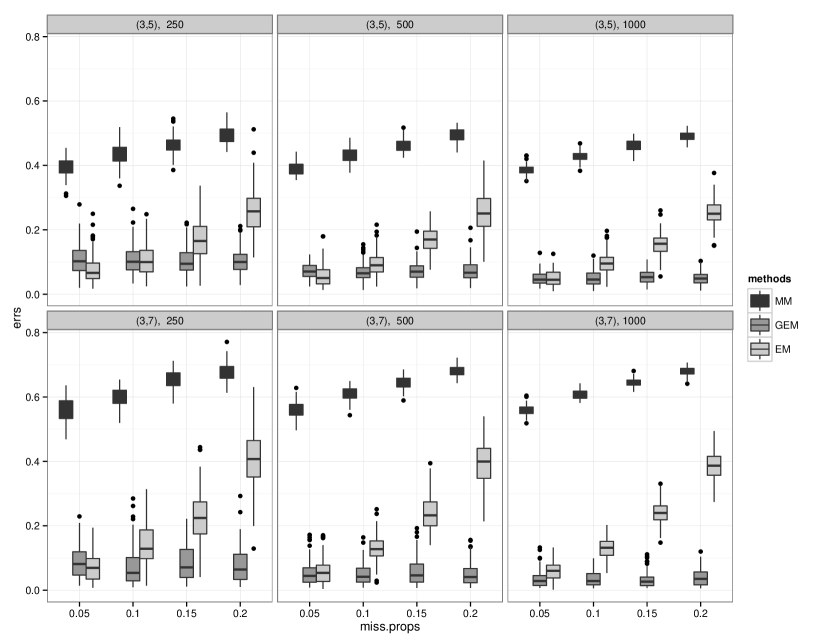
Figure 1. Boxplots of the relative errors in the estimates of $\Sigma$, in order of $MM$, $GEM$, and $EM$.

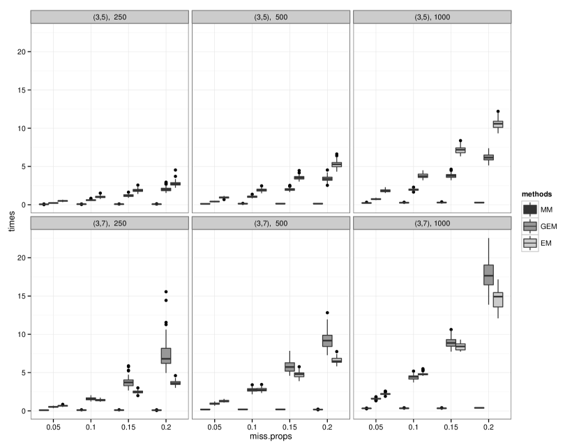
Figure 2. Boxplots of the run times (in seconds), in order of $MM$, $GEM$, and $EM$.

The relative errors of the mean estimates across the three methods and the four different proportions of missing data were consistently low. The methods differ very little when it comes to the estimate of the mean, and so we focus on the variance estimates. Indeed, the models and estimation procedure vary most when dealing with the covariance matrix.

Figure 1 tells a rich story about how these three methods differ most. Since the $MM$ method essentially treats the imputed values as actual data and fails to account for all of the uncertainty present, the errors for this method top all of those from the $GEM$ and $EM$. As the sample size increases the estimates appear to improve slightly, but the most interesting feature lies in the difference between the $GEM$ and $EM$ methods. Since (6) contains more parameters to be estimated, this model can achieve better resolution and accuracy than (5), albeit needing more samples to identify parameters. The significant cost lies in the computation time, making the kronecker structure a worthwhile consideration since it noticeably reduces the complexity of the model and still achieves accurate parameter estimates.

Figure 2 introduces the computational differences between the methods. The $MM$ method, while still requiring some iterating, takes very little time in all scenarios. Interestingly, the $EM$ method requires the most time for lower dimensions such as the $p=3$, $q=5$ situation simulated here. When the dimensions increase, we begin to see the gains in the kronecker model. Naturally, as the discrepancy in the number of parameters being estimated by $GEM$ and $EM$ increases, the computational advantages become more significant. Additionally, the difference in sample sizes necessary to estimate the covariance grows, with $GEM$ requiring more.

Of course, this presumes the choice between the two models. In a situation where the physical dimensions of the data imply a kronecker structure, we can take comfort in the above results. One such example is the following application to Remote Sensing.

3.2. Land Cover Classification using MODIS Satellite Image Data

One of the biggest tasks in Remote Sensing is land-cover classification. In other words, taking remotely sensed images composed of millions of pixels and assigning to each pixel a particular land cover class. Many of the richest datasets are both multispectral and multitemporal. For satellite image data from the MODIS device we observe data in 7 different spectral bands at each of 46 time points (comprising a multivariate annual profile). The analysis we present here is an application of the proposed EM algorithm to these multivariate time series data. We adopt the following model:

(11) $${\mbox{\rm vec}}(X_{v}){\,|\,}\theta_{v}=c\sim N({\mbox{\rm vec}}(\mu_{c}),\sigma^{2}_{c}\Sigma_{c}\otimes\Sigma_{s}),$$

where $X_{v}$ and $\theta_{v}$ are the data and land cover class for pixel $v$, respectively. In this geographical context the kronecker structure naturally models the covariance in the spectral bands ($\Sigma_{s}$) and the covariance in time for each class ($\Sigma_{c}$). That is, the full covariance is partitioned into spectral and temporal components. Note that in (11) we allow for a different mean, temporal covariance and scale ($\sigma^{2}$) for each class.

For geographical reasons we focus our attention on the middle of the year (the middle 28 time points). Thus $X$ and $\mu_{c}$ are $7\times 28$ matrices, $\Sigma_{c}$ is a $28\times 28$ matrix and $\Sigma_{s}$ is a $7\times 7$ matrix. For the analysis that follows we used a subset of the MODIS Land Cover Training site database that includes 204 sites located over the conterminous United States. These sites include 2,245 MODIS pixels and encompass most major biomes and land cover types in the lower 48 United States (Schaaf et al, 2002).

Land cover classification has been approached in many different ways for quite some time. The high dimensionality of the data presents an increasingly significant challenge. Traditionally, principal components analysis (PCA) has been used to reduce the dimensionality of the data. However, usually all 196 ($7\cdot 28$) features are considered distinct features. Consequently, spectral and temporal variation cannot be isolated from an eigen-decomposition of the full ($196\times 196$) covariance matrix, as required from PCA.

To preserve the raw temporal information and still reduce the dimensionality of the data, we propose targeting $\Sigma_{s}$ with the principal components analysis as opposed to $\Sigma_{c}\otimes\Sigma_{s}$. About 5% of the data is missing, making the kronecker structure and our proposed EM algorithm even more ideal, from a purely computational standpoint, as evidenced by the simulation study above. Using the proposed EM algorithm we estimate the parameters of (11) and perform PCA on our estimate of $\Sigma_{s}$. To, again, provide a comparison which confirms the quality of our $EM$ we compare the PCA results just described to those computed using the $MM$ method.

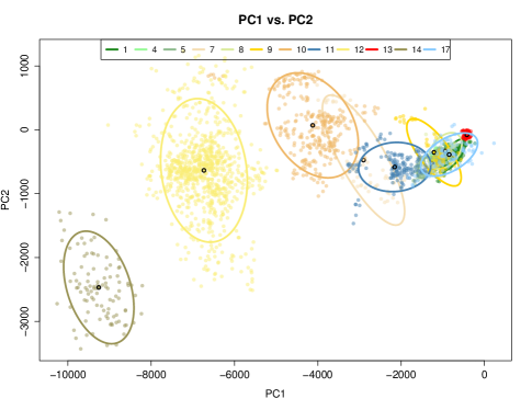
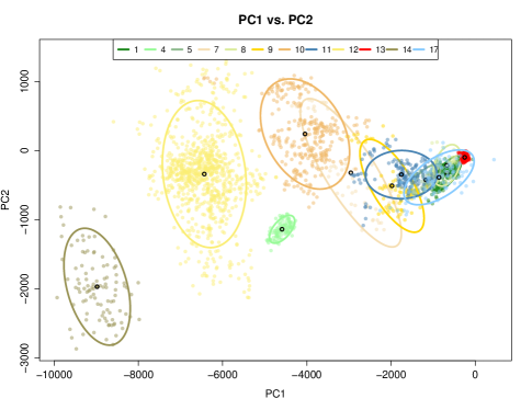
Figure 3. Left: the data projected into the space of the first two principal components, colored by their respective land color classes; right: hierarchical clustering of classes. Top and bottom panels: results using MM and EM, respectively.

Figure 3 shows the data projected into the space of the first two principal components using the $MM$ and $EM$ methods. The class separability seems reasonable and the different amounts of variation in each class are certainly identified. A closer inspection reveals that the $EM$ method achieves better separability of the land-cover classes. This can be seen in the PC1 versus PC2 plots as well as their neighboring dendrograms. These dendrograms resulted from a hierarchical clustering of the classes using the following distance metric, $d_{ij}$:

$$d_{ij}=(\mu_{i}-\bar{\mu}_{ij})^{\top}\Sigma_{i}^{-1}(\mu_{i}-\bar{\mu}_{ij})+(\mu_{j}-\bar{\mu}_{ij})^{\top}\Sigma_{j}^{-1}(\mu_{j}-\bar{\mu}_{ij}).$$

where the $\bar{\mu}_{ij}$ are “in-between” centers for clusters $i$ and $j$,

$$\bar{\mu}_{ij}=\Sigma_{i}^{-1}(\Sigma_{i}^{-1}+\Sigma_{j}^{-1})^{-1}\mu_{i}+\Sigma_{j}^{-1}(\Sigma_{i}^{-1}+\Sigma_{j}^{-1})^{-1}\mu_{j}.$$

The log distances are plotted above along with an overall log distance, $D=\sum_{i<j}d_{ij}$. As a measure of the overall separability of the classes in the space of the first two principal components, the greater value of $\log(D)$ achieved by the $EM$ confirms that this method helped to better distinguish land-cover classes.

In particular, using the $EM$, the first two principal components capture 76.1% of the variation in the spectral bands. For the purposes of land-cover classification we chose to use the first three principal components since they capture 92.3% of the variation in the spectral bands.

A simple MLE classification for each pixel based on these PCs yielded an accuracy of 66.9%. Though 66.9% might be considered low and significant overlap of the classes appears to exist in the bottom panel of Figure 3, this accuracy and overlap are expected to some degree due to the nature of the data and ambiguity in some of the class definitions. So, these results are pleasing.

4. Conclusion

The matrix normal distribution is a natural candidate for situations involving some sort of structure or separability in the dimensions of the data. In this article we derived an expectation-maximization algorithm for the matrix normal distribution. A simulation study exploring different sample sizes and proportions of missing data showed the usefulness and shortcomings of this method when compared to a full, unconstrained multivariate normal distribution. An example of this type of scenario, in the field of Remote Sensing, produced physically useful and interpretable results. As data becomes more abundant and higher in dimension the challenge of extracting information continues to grow in difficulty and importance. The kronecker covariance structure can provide both a richer physical interpretation of the parameters as well as help the estimating procedure. Now, even with missing data, accurate estimates of these parameters are obtainable.

Appendix A EM Algorithm for Matrix Normal

Here we give a more detailed implementation of the proposed EM method in Algorithm 1. In what follows, the operator ${\textbf{e}}(\cdot)$ produces a mask matrix according to the corresponding row and column indices. Take the following example:

$$X_{i}=\left[\begin{array}[]{ccccccc}1&4&7&10&?&16&?\\ ?&5&8&11&14&17&20\\ ?&6&?&12&15&?&21\end{array}\right].$$

There are six missing values that correspond to $m_{s}(i)=[2\,3\,3\,1\,3\,1]$ and $m_{c}(i)=[1\,1\,3\,5\,6\,7]$. In this case, ${\textbf{e}}(m_{c}(i))$ is $6\times 7$ (the number of missing values by the number of columns of $X$) and ${\textbf{e}}(m_{s}(i))$ is $6\times 3$ (the number of missing values by the number of rows of $X$):

$${\textbf{e}}(m_{c}(i))=\left[\begin{array}[]{ccccccc}1&0&0&0&0&0&0\\ 1&0&0&0&0&0&0\\ 0&0&1&0&0&0&0\\ 0&0&0&0&1&0&0\\ 0&0&0&0&0&1&0\\ 0&0&0&0&0&0&1\end{array}\right]\quad\text{and}\quad{\textbf{e}}(m_{s}(i))=\left[\begin{array}[]{ccc}0&1&0\\ 0&0&1\\ 0&0&1\\ 1&0&0\\ 0&0&1\\ 1&0&0\end{array}\right].$$

In this way, there is an “indicator” row for each index in $m_{c}(i)$ and $m_{s}(i)$, respectively.

In Algorithm 1 we denote by $\circ$ the Hadamard (element-wise) product. We further denote by $A[m_{s}(i)]$ the rows of $A$ indexed by $m_{s}(i)$, and by $A[-m_{s}(i)]$ the rows of $A$ there are not in $m_{s}(i)$. A similar notation is used to subset columns based on index sets.

Initialize: $\mu^{(1)}\leftarrow 0_{p\times q}$; $\Sigma_{c}^{(1)}\leftarrow I_{q}$; $\Sigma_{s}^{(1)}\leftarrow I_{p}$;

for $t\leftarrow 1,\ldots$ (until convergence) do

       $\mu^{(t+1)}\leftarrow 0_{p\times q}$; $\Sigma_{c}^{(t+1)}\leftarrow 0_{q}$; $\Sigma_{s}^{(t+1)}\leftarrow 0_{p}$;

      

      for $i\leftarrow 1,\ldots,n$ do

             // Initialize missing entry indices and conditional covariance:

             Set miss$(i)$ as the indices of missing entries in the $i$-th observation;

            

            Set $m_{s}(i)$ and $m_{c}(i)$ as the row and column indices of the entries in miss$(i)$;

            

            SWEEP the miss$(i)$ rows of $R=\Sigma_{c}^{-1^{(t)}}\otimes\Sigma_{s}^{-1^{(t)}}$ ;

              // Compute ${\mbox{\rm Var}}_{Z_{i}{\,|\,}Y_{i}}[X_{i}]$

            

            

            // Set auxiliary variables:

             $X_{m}\leftarrow\left[\begin{array}[]{c}Y_{i}\\ \mu^{(t)}[\text{\sf miss}(i)]+R[-\text{\sf miss}(i),\text{\sf miss}(i)]^{\top}(Y_{i}-\mu^{(t)}[-\text{\sf miss}(i)])\end{array}\right]$ ;

              // ${\mathbb{E}}_{Z_{i}{\,|\,}Y_{i}}[X_{i}]$

            

            $R_{m}\leftarrow R[\text{\sf miss}(i),\text{\sf miss}(i)]$;

            

            $S_{s,m}\leftarrow\Sigma_{s}^{-1^{(t)}}[m_{s}(i),m_{s}(i)]$;

            

            $S_{c,m}\leftarrow\Sigma_{c}^{-1^{(t)}}[m_{c}(i),m_{c}(i)]$;

            

            

            // Update:

             $\mu^{(t+1)}\leftarrow\mu^{(t+1)}+X_{m}$;

            

            $\Sigma_{c}^{-1^{(t+1)}}\leftarrow\Sigma_{c}^{-1^{(t+1)}}+{\textbf{e}}(m_{c}(i))^{\top}\cdot(R_{m}\,\circ\,S_{c,m})\cdot{\textbf{e}}(m_{c}(i))+(X_{m}-\mu^{(t)})^{\top}\Sigma_{s}^{-1^{(t)}}(X_{m}-\mu^{(t)})$;

            

            $\Sigma_{s}^{-1^{(t+1)}}\leftarrow\Sigma_{s}^{-1^{(t+1)}}+{\textbf{e}}(m_{s}(i))^{\top}\cdot(R_{m}\,\circ\,S_{s,m})\cdot{\textbf{e}}(m_{s}(i))+(X_{m}-\mu^{(t)})\Sigma_{c}^{-1^{(t)}}(X_{m}-\mu^{(t)})^{\top}$;

            

            $\sigma^{2^{(t+1)}}\leftarrow\sigma^{2^{(t+1)}}+\sum_{j}{\mbox{\rm vec}}{(R_{m}\,\circ\,S_{c,m}\,\circ\,S_{s,m})}+{\mbox{\rm tr}}({\mbox{\rm vec}}{(X_{m}-\mu^{(t)})^{\top}}(\Sigma_{c}^{-1^{(t)}}\otimes\Sigma_{s}^{-1^{(t)}}){\mbox{\rm vec}}{(X_{m}-\mu^{(t)})})$;

            

       end for

      

      

      // Scale:

       $\mu^{(t+1)}\leftarrow\mu^{(t+1)}/n$;

       $\Sigma_{c}^{(t+1)}\leftarrow\Sigma_{c}^{(t+1)}/\Sigma_{c,11}^{(t+1)}$;

       $\Sigma_{s}^{(t+1)}\leftarrow\Sigma_{s}^{(t+1)}/\Sigma_{s,11}^{(t+1)}$;

       $\sigma^{2^{(t+1)}}\leftarrow\sigma^{2^{(t+1)}}/(nBT)$;

      

end for

Algorithm 1 Matrix Normal Expectation-Maximization

References

- Boik (1991) Boik JB (1991) Scheffe’s mixed model for multivariate repeated measures: A relative efficiency evaluation. Communications in Statistics - Theory and Methods 20:1233–1255
- Chaganty and Naik (2002) Chaganty NR, Naik DN (2002) Analysis of multivariate longitudinal data using quasi-least squares. Journal of Statistical Planning and Inference 103:421–436
- Dawid (1981) Dawid AP (1981) Some matrix-variate distribution theory: Notational considerations and a bayesian application. Biometricka 68(1):265–274
- Dempster et al (1977) Dempster A, Laird N, Rubin D (1977) Maximum likelihood from incomplete data via the em algorithm. Journal of the Royal Statistical Society 39:1–38
- Dutilleul (1999) Dutilleul P (1999) The MLE algorithm for the matrix normal distribution. Journal of Statistical Computation and Simulation 64(2):105–123
- Friedl et al (2009) Friedl MA, et al (2009) Modis collection 5 global land cover: Algorithm refinements characterization of new datasets. Remote Sensing of Environment 114:168–182
- Fuentes (2004) Fuentes M (2004) Testing for separability of spatial-temporal covariance functions. Journal of Statistical Planning and Inference 136:447–466
- Galecki (1994) Galecki AT (1994) General class of covariance structures for two or more repeated factors in longitudinal data analysis. Communications in Statistics - Theory and Methods 23(11):3105–3119
- Goodnight (1979) Goodnight JH (1979) A tutorial on the SWEEP operator. The American Statistician 33(3):149–158
- McLachlan and Krishnan (1997) McLachlan GJ, Krishnan T (1997) The EM Algorithm and Extensions. Wiley Series in Probability and Statistics
- Naik and Rao (2001) Naik DN, Rao S (2001) Analysis of multivariate repeated measures data with a kronecker product structured covariance matrix. Journal of Applied Statistics 28:91–105
- Petersen and Pedersen (2008) Petersen KB, Pedersen MS (2008) The matrix cookbook
- Roy and Khattree (2005) Roy A, Khattree R (2005) On discrimination and classification with multivariate repeated measures data. Journal of Statistical Planning and Inference 134(2):462–485
- Roy A. (2005) Roy A KR (2005) Testing the hypothesis of a kroneckar product covariance matrix in multivariate repeated measures data. Statistical Methodology 2
- Schaaf et al (2002) Schaaf C, et al (2002) First operational brdf, albedo nadir reflectance products from modis. Remote Sensing of Environment 83(1):135–148
- Shitan and Brockwell (1995) Shitan M, Brockwell PJ (1995) An asymptotic test for separability of a spatial autoregressive model. Communications in Statistics - Theory and Methods 24(8):2027–2040
- Srivastava and Khatri (1979) Srivastava M, Khatri C (1979) An Introduction to Multivariate Statistics. North Holland, New York, USA
- Srivastava et al (2008) Srivastava M, Nahtman T, von Rosen D (2008) Models with a Kronecker product covariance structure: Estimation and testing. Mathematical Methods of Statistics 17(4):357–370