Reconstructing primordial power spectrum using Planck and SDSS-III measurements

Abstract

We develop an accurate and efficient Bayesian method to reconstruct the primordial power spectrum in a model-independent way, and apply it to the latest cosmic microwave background measurement from Planck mission, and the large scale structure observation of SDSS-III BOSS (CMASS) sample, combined with the type Ia supernovae sample (SNLS 3-year) and the measurements of baryon acoustic oscillations from SDSS-II, 6dF, and WiggleZ survey. We confirm that the scale-invariant primordial power spectrum is strongly disfavored, and a model with suppressed power on horizon scales is supported by current data. We also find that a modulation on scales $5\times 10^{-4}~{}\textrm{Mpc}^{-1}\lesssim k\lesssim 0.01~{}\textrm{Mpc}^{-1}$ is mildly preferred at $2\sigma$ confidence level, whose origin needs further investigation.

The reconstruction of the primordial power spectral amplitude $A_{s}(k)$ directly from cosmological observations provides the key to understanding the physics of the early universe. A scale-dependent $A_{s}(k)$, if confirmed, clearly supports the inflation paradigm, and thus various inflationary models can be differentiated by the specific scale-dependence, e.g., the large-scale modulations and the small-scale features. This theoretical significance has motivated many efforts in the literature to reconstruct $A_{s}(k)$ either parametrically (more often using a power-law parametrization), or non-parametrically.

Non-parametric reconstruction of $A_{s}(k)$ is receiving more and more attention since the result can be largely immune to theoretical bias because no ad hoc functional form of $A_{s}(k)$ needs to be assumed, which is inevitable in parametric approaches. However, accurate and efficient non-parametric methods are in general difficult to design and implement because it needs to satisfy some requirements. For instance, (I) it should allow a sufficient number of degrees of freedom (d.o.f.’s) to find significant large- and small-scale features in $A_{s}(k)$, if there are any, (II) it must not over-fit data, i.e., avoidance of fitting noise, (III) it should include reconstruction error analysis, favorably in Bayesian nature, (IV) other cosmological parameters can be varied simultaneously to account for parameter degeneracies and (V) it should be applicable to any kinds of data, including geometrical indicators, e.g., baryon acoustic oscillations (BAO), type Ia supernovae (SNIa).

A lot of methods have been proposed in the spirit of binning binning , i.e., fitting constant values of $A_{s}(k)$ in several $k$ bins to data. These methods can in principle satisfy (III) and (IV), but it is difficult to have sufficient number of bins due to parameter degeneracies. Direct inversion methods cosmic_inversion can solve this problem, but they in general do not satisfy (III-V). Fitting principle components is less affected by parameter degeneracies Leach:2005av , but zeroing the poorly-constrained high frequency modes, which is practically necessary when employing the Markov Chain Monte Carlo (MCMC) method, can bias the reconstruction result in a non-trivial way Huterer:2002hy . The multi-resolution methods, including the direct wavelet expansion wavelet , are promising in feature detection, yet it is difficult to avoid under- or over-fitting data. The methods with a penalty term in likelihood calculation are designed to avoid data over-fitting, but using a few fitting nodes with interpolation Sealfon:2005em might artificially smooth out signals, hence violates (I), while the method developed in Gauthier:2012aq and applied in planck:inflation can hardly satisfy (IV) and (V).

In this work, we employ the correlated prior method recently developed for dark energy equation of state reconstruction cpz1 ; cpz2 ; cpz3 to reconstruct the primordial power spectrum using mainly Planck 2013 planck:cosmology and SDSS-III BOSS measurements boss . This non-parametric Bayesian reconstruction technique satisfies rigorously all the requirements (I-V).

Suppose $A_{s}(k)$ is a Gaussian random field with a covariance described by a correlation function,

$$\xi(|\kappa-\kappa^{\prime}|)\equiv\left\langle[A_{s}(\kappa)-A_{s}^{\rm fid}(\kappa)][A_{s}(\kappa^{\prime})-A_{s}^{\rm fid}(\kappa^{\prime})]\right\rangle$$ (1)

where $\kappa\equiv\ {\rm ln}\ k$. Discretizing $A_{s}(\kappa)$ into $N_{\kappa}$ bins in the range of $[\kappa_{\rm min},\kappa_{\rm max}]$, one can calculate the $\{i,j\}$ component of the covariance matrix for the correlated prior,

$$C_{ij}=\frac{1}{\Delta^{2}}\int_{\kappa_{i}}^{\kappa_{i}+\Delta}{\rm d}\kappa\int_{\kappa_{j}}^{\kappa_{j}+\Delta}{\rm d}\kappa^{\prime}~{}\xi(|\kappa-\kappa^{\prime}|)$$ (2)

where $\Delta$ is the bin width. We adopt the CPZ form for the correlation function due to its relatively simple behavior and transparent dependence on its parameters cpz2 , i.e., $\xi(\delta\kappa)=\xi(0)/[1+(\delta\kappa/\kappa_{c})^{2}]$, where $\kappa_{c}$ determines the correlation length and the amplitude $\xi(0)$ sets the strength of the prior. The variance of the mean $A_{s}$ over all the bins simply follows from Eq. (2) when taking $i=j$ and $\Delta$ to be the entire $\kappa$ interval, and in the limit of $\kappa_{c}\ll\kappa_{\rm max}-\kappa_{\rm min}$, this variance can be calculated as,

$$\sigma^{2}_{\bar{P}}=\int_{\kappa_{\rm min}}^{\kappa_{\rm max}}\int_{\kappa_{\rm min}}^{\kappa_{\rm max}}\frac{{\rm d}\kappa{\rm d}\kappa^{\prime}~{}\xi(\kappa-\kappa^{\prime})}{(\kappa_{\rm max}-\kappa_{\rm min})^{2}}\simeq\frac{\pi\xi(0){\kappa_{c}}}{\kappa_{\rm max}-\kappa_{\rm min}}$$ (3)

A strong prior (large $\kappa_{c}$, small $\sigma^{2}_{\bar{P}}$, hence small $\xi(0)$) results in small variance of the reconstruction, but may bias the reconstructed model when the true model is in tension with the peak of the prior. Using a much weaker prior can avoid biasing the result, but it inevitably leads to a very noisy reconstruction, in other words, over-fit data. To find reasonable values for the prior, we perform tests on an ensemble of inflationary models with different potentials, and we find that taking $\sigma^{2}_{\bar{P}}=0.072,\kappa_{c}=0.6$ yields accurate reconstruction with negligible bias. We take this prior to be the ‘standard’ prior. To be conservative, we also consider a ‘weak’ prior with $\sigma^{2}_{\bar{P}}=0.144,\kappa_{c}=0.6$ in case that the true $A_{s}$ is not covered by the suite of models we use for the bias test.

The correlated prior for the model is then

$$\mathcal{P}_{{\rm prior}}\propto{\rm exp}\left[-\left(\mathbf{A_{s}}-\mathbf{A_{s}^{{\rm fid}}}\right)^{T}\mathbf{C}^{-1}\left(\mathbf{A_{s}}-\mathbf{A_{s}^{{\rm fid}}}\right)/2\right]$$ (4)

To incorporate this prior with MCMC, we minimize the total posterior $\chi^{2}\equiv\chi_{\rm data}^{2}+\chi_{{\rm prior}}^{2}$ where $\chi_{{\rm prior}}^{2}=-2\ {\rm ln}\ \mathcal{P}_{{\rm prior}}$. As discussed in cpz2 , the correlated prior can effectively gauge the flat directions in parameter space, which enables MCMC calculations to converge even for a large number of bins. This allows for a high-resolution reconstruction of $A_{s}(\kappa)$ without over-fitting data since the correlated prior penalizes the high-frequency modes in such a fashion that the oscillatory modes with low significance are effectively washed out, while the features with high significance, including those sharp ones, are not affected by the prior.

To avoid biasing the result by assuming any fiducial model $A_{s}^{\rm fid}$ in Eq. (4), we marginalize over it following cpz2 ; cpz3 to take local average of the neighboring trial bins within a range of $\Delta\kappa=\kappa_{c}=0.6$. We have checked our result by adopting another marginalization method of panelizing ${\rm d}A_{s}/{\rm d\kappa}$ instead cpz3 , and found a consistent result.

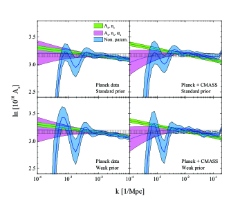
Figure 1: The best fit (solid curves) and 68% CL error (shaded bands) of the reconstructed primordial power spectrum using the power law parametrization (green and purple shaded) and free-form with correlated priors (blue shaded). Different datasets and priors are employed as illustrated in the legends. The horizontal bands with patterns show the 68% CL constraint on the HZ model.

In practice, we fit ln$A_{s}(\kappa)$ to data since it is closer to Gaussian distribution. We approximate ln$A_{s}(\kappa)$ using 40 bins $\mathcal{A_{S}}\supset\{{\rm ln}A_{s}({\kappa_{i}}),\ i=1,...,40\}$, spaced uniformly in $\kappa$ in the range of $[{\rm ln}10^{-4},{\rm ln}0.3]$, to cover the range of observables we use. The bin width is sufficiently small compared to the correlation length, thus the prior largely wipes out the dependence on the choice of binning. For comparison, we also fit the usual power law model to data, namely,

$${\rm ln}A_{s}(k)={\rm ln}A_{s}+(n_{s}-1)~{}{\rm ln}(k/k_{0})+\frac{\alpha_{s}}{2}~{}{\rm ln}(k/k_{0})^{2}$$ (5)

where $A_{s},n_{s}$ and $\alpha_{s}$ are constants and $k_{0}$ is the pivot scale of $0.05$ Mpc^-1. So in this case $\mathcal{A_{S}}\supset\{{\rm ln}A_{s},n_{s},\alpha_{s}\}$.

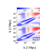
Figure 2: (A1): The correlation matrix among the $\kappa$ bins obtained in MCMC using Planck data, subtracted off that of the weak correlated prior; (A2): same as (A1) but for Planck+CMASS data; (B): selected eigen-modes of the covariance matrix obtained using Planck+CMASS data with a weak correlated prior; (C): The eigen-values of the covariance matrix obtained using Planck, Planck+CMASS data with a weak correlated prior, and that of the weak correlated prior itself; (D1,2): The improved ln$L$ of the binned model with a weak correlated prior (black dashed); The logarithmic fractional volume ln$V$ of the sampled parameter space (red dash-dot); The logarithmic evidence (blue solid). All three curves are for the residue with respect to that of the constant $A_{s}$ model as a function of the diagonal prior $\sigma_{\rm bin}$. See text for more details. (D1) and (D2) are for Planck and Planck+CMASS data respectively.

We apply our method to a joint dataset of the latest cosmological observations. The cosmic microwave background (CMB) and galaxy power spectrum have direct information for $A_{s}(\kappa)$ and therefore we use the first year CMB measurement from Planck satelliteplanck:cosmology and the 3D galaxy power spectrum of SDSS-III BOSS DR9, the CMASS sample boss . We model the galaxy bias and the redshift space distortion using the approach developed in Cole:2005sx and applied to CMASS in Zhao:2012xw . We also include other measurements to constrain the background cosmology to break parameter degeneracies. We use the BAO measurements from SDSS-II sdss2 , 6dF 6df and WiggleZ survey wigglez , and the SNIa sample of SNLS 3-year Conley:2011ku . Note that we didn’t combine the $H_{0}$ measurement in Riess:2011yx because of its tension with Planck data. Given this joint dataset, we use MCMC Lewis:2002ah to sample the parameter space ${\bf P}\equiv(\omega_{b},\omega_{c},\Theta_{s},\tau,\mathcal{A_{S}},\mathcal{N})$ where $\omega_{b}$ and $\omega_{c}$ are the baryon and cold dark matter densities, $\Theta_{s}$ is the ratio of the sound horizon to the angular diameter distance at decoupling, and $\tau$ is the optical depth. We also include and marginalize over $\mathcal{N}$, which represents the 14 nuisance parameters involved with the Planck CMB likelihood and another 2 accounting for the calibration uncertainty in measuring the intrinsic SN luminosity. A modified version of CAMB CAMB is used to calculate the observables. Note all the above parameters are simultaneously varied in our reconstruction.

The reconstruction result is shown in Fig. 1. The blue shaded regions on top layers in four panels illustrate the 68% confidence level (CL) uncertainties of our reconstruction, while the solid curves inside the bands show the best fit $\mathcal{A_{S}}$ models. The reconstructions using different correlated priors (standard and weak) and diverse data combinations (Planck and Planck+CMASS) are displayed separately. Here the datasets of SNIa and BAO are always utilized throughout our analysis. In all cases, we can identify a significant signal of the lack of power on large scales ($k\lesssim 5\times 10^{-4}$ Mpc^-1), which is also apparent in the Planck CMB data. Interestingly, we find a sign of modulation on scales $5\times 10^{-4}~{}\textrm{Mpc}^{-1}\lesssim k\lesssim 0.01~{}\textrm{Mpc}^{-1}$. Adding the CMASS sample makes the modulation slightly less significant, but still obvious. For a comparison, we also show the reconstructions assuming the usual power-law parametrization, i.e., Eq. (5). The purple or green shaded bands represent the cases in which the running $\alpha_{s}$ is fixed to 0 or allowed to vary respectively, with the corresponding best fit models plotted within their bands. We also did another fit for the Harrison-Zel’dovich (HZ) model, i.e., $n_{s}=1,~{}\alpha_{s}=0$ (shown in horizontal bands with patterns). In all cases, we can see that the power-law reconstructions are in agreement with the free-form ones on scales of $5\times 10^{-3}~{}\textrm{Mpc}^{-1}\lesssim k\lesssim 0.1~{}\textrm{Mpc}^{-1}$. On larger scales $k\lesssim 5\times 10^{-3}$ Mpc^-1, the power law reconstructions fail to capture the suppression of power, and the modulation. This is expected due to the lack of d.o.f.’s in the power-law form. Interestingly, from Table I we see that the inclusion of CMASS data changes mean values of the tilt $n_{s}$ from 0.9653 to 0.9500 ($\alpha_{s}$ fixed to 0) and from 0.9620 to 0.9477 ($\alpha_{s}$ float) respectively. Moreover, Planck+CMASS data mildly favors a non-zero running at about $2.3\sigma$. The origin of this inconsistency between two datasets is unclear, and asks for further investigation.

	Data Combinations
	Planck	Planck+CMASS
ln$(10^{10}\ A_{s})$	$3.137\pm 0.031$	$3.181\pm 0.033$
ln$(10^{10}\ A_{s})$	$3.091\pm 0.026$	$3.098\pm 0.024$
$n_{s}$	$0.9653\pm 0.0057$	$0.9500\pm 0.0053$
ln$(10^{10}\ A_{s})$	$3.110\pm 0.032$	$3.139\pm 0.031$
$n_{s}$	$0.9620\pm 0.0063$	$0.9477\pm 0.0059$
$\alpha_{s}$	$-0.0128\pm 0.0090$	$-0.0205\pm 0.0088$

Table 1: The mean and 68% CL error of the power-law parameters when they vary.

To quantify the goodness of fit using different parametrisations, we list the $\chi^{2}$ for the corresponding best fit models relative to that for the HZ model in Table II. We can see that the HZ model is strongly disfavored in all cases, with the significance ranging from $5.6\sigma$ (Planck, $n_{s}$ float, $\alpha_{s}$ fixed) to $9.6\sigma$ (Planck+CMASS, weak prior). For the power law scenario with Planck+CMASS, $\chi^{2}$ can be reduced by $12.5$ if $\alpha_{s}$ is allowed to vary, which is consistent with what we see in Table I: a non-zero running is unambiguously preferred by this data combination. If we allow additional d.o.f.’s, i.e., adopting the free-form parametrization, $\chi^{2}$ can be drastically reduced. For example, with Planck+CMASS, $\chi^{2}$ for the weak prior case is lower than the power law case with free running by $16.1$, which is a $4\sigma$ significance.

	Power Law		Free-Form
	$n_{s}$	$n_{s},~{}\alpha_{s}$	Standard Prior	Weak Prior
Planck	$-31.5$	$-32.4$	$-47.6$	$-51.7$
Planck+CMASS	$-64.1$	$-76.6$	$-83.7$	$-92.7$

Table 2: The improved $\chi^{2}$ of the power law and free-form models with respect to the Harrison-Zel’dovich model ($n_{s}=1$) using two datasets (Planck and Planck+CMASS).

To understand this result and confirm that we are not over-fitting data, we perform a principle component analysis and calculate the Bayes factor explicitly. We diagonalise the covariance matrix for the $\mathcal{A_{S}}$ bins, which is obtained from the posterior distribution, in order to find the uncorrelated linear combinations of the bins with all other cosmological parameters marginalized over. Panels (A1, A2) in Fig. 2 show the correlation matrix (the normalized covariance matrix so that all the diagonal terms are $1$) among the bins subtracted off the weak prior correlation matrix for Planck and Planck+CMASS data respectively. Note that if data are absent, the correlated prior provides a positive correlation among bins within the correlation length, so the prior correlation matrix is block diagonal with positive entries in the off-diagonal terms. When data are added in, this correlation pattern can be changed significantly where data are strong, or not affected much where data are weak. From (A1, A2) we can recognize that data require negative correlation among bins on scales $k\lesssim 0.01$ Mpc^-1, meaning that a large variation of amplitudes on these scales is favored. This is consistent with what we see in Fig. 1. On smaller scales, the correlation is positive, suggesting that amplitudes on these scales behave more coherently, and this is the reason that there is no apparent features seen on these scales in our reconstruction. The inclusion of CMASS data slightly changes the correlation pattern, e.g., the correlation on quasi-nonlinear scales ($0.1~{}\textrm{Mpc}^{-1}\lesssim k\lesssim 0.2~{}\textrm{Mpc}^{-1}$) is more negative, implying a feature on such scales, which is seen in Fig. 1. However, this feature is likely due to systematics, e.g., issues of nonlinearity rather than being physical.

Panels (B, C) show the eigen-vectors and eigen-values of the covariance matrix. From panel (B), we see that the well constrained modes modulate on scales where we see features in the reconstruction, and panel (C) quantitatively shows that Planck and Planck+CMASS can constrain 8 and 10 such modes respectively.

Our free-form reconstructions apparently fit data better than the HZ or the power-law models, but the key issue is whether this is ascribed to an over-fit of the data, in other words, whether this fitting improvement can compensate for the increased volume of parameter space. This can be quantified by computing the Bayes factor $E$ within a family of models interpolating smoothly between the weak prior free-form model and the HZ model. We follow cpz3 and implement this via adding a larger and larger diagonal term to the inverse prior matrix which effectively reduces the variance in each bin. This essentially shifts all the eigen-values by a constant. The Bayes factor $E$ can be estimated as,

$$E\propto VL;~{}V=\sqrt{\frac{\det{{\cal C}_{\rm post}}}{\det{{\cal C}_{\rm prior}}}};~{}L=e^{-\chi_{\rm b.f.}^{2}/2},$$ (6)

where ${\bf{\cal{C}}}_{\rm prior}$ and ${\bf{\cal{C}}}_{\rm post}$ denote the prior and posterior covariance matrices respectively, and $\chi_{\rm b.f.}^{2}$ is the $\chi^{2}$ for the best fit model given the combination of data and prior. Note that $V$ quantifies the fraction of the parameter space corresponding to the initial prior consistent with data, while $L$ indicates how well the model is capable of fitting the data. Panels (D1, D2) in Fig. 2 show ${\rm ln}L,~{}{\rm ln}V$ and ${\rm ln}E$ with respect to those in the HZ model as a function of $\sigma_{\rm bin}$ calculated using Planck and Planck+CMASS data respectively. As we see, $\Delta{\rm ln}E$ is non-negative for all $\sigma_{\rm bin}$, inferring the necessity of free-form reconstructions of $A_{s}(k)$. Especially when $\sigma_{\rm bin}$ approaches 20, which corresponds to the weak prior model, $\Delta{\rm ln}E$ is $16.1$ and $26.4$ for Planck and Planck+CMASS respectively.

In this letter, we develop a new and robust Bayesian method to reconstruct the primordial power spectrum in a non-parametric way using latest cosmological observations including Planck and SDSS-III measurements. We find that the scale-invariant spectrum is strongly disfavored, while a model with suppressed power on large scales ($k\lesssim 5\times 10^{-4}$ Mpc^-1) is supported by data. A sign of modulation on scales $5\times 10^{-4}~{}\textrm{Mpc}^{-1}\lesssim k\lesssim 0.01~{}\textrm{Mpc}^{-1}$ is also evidenced by current CMB and large scale structure data. Whether it stems from new physics in the early universe Feng:2003zua or some unaccounted systematics can be shed light upon with the upcoming polarization data from Planck and future large redshift surveys.

- (1) S. L. Bridle, A. M. Lewis, J. Weller and G. Efstathiou, Mon. Not. Roy. Astron. Soc. 342, L72 (2003); M. Bridges, A. N. Lasenby and M. P. Hobson, Mon. Not. Roy. Astron. Soc. 381, 68 (2007); R. Hlozek et al., Astrophys. J. 749, 90 (2012).
- (2) M. Matsumiya, M. Sasaki and J. ’i. Yokoyama, Phys. Rev. D 65, 083007 (2002); M. Matsumiya, M. Sasaki and J. ’i. Yokoyama, JCAP 0302, 003 (2003); N. Kogo, M. Matsumiya, M. Sasaki and J. ’i. Yokoyama, Astrophys. J. 607, 32 (2004). A. Shafieloo and T. Souradeep, Phys. Rev. D 70, 043523 (2004); A. Shafieloo and T. Souradeep, Phys. Rev. D 78, 023511 (2008); D. Tocchini-Valentini, M. Douspis and J. Silk, Mon. Not. Roy. Astron. Soc. 359, 31 (2005); P. Hunt and S. Sarkar, JCAP 01, 025 (2014).
- (3) S. M. Leach, Mon. Not. Roy. Astron. Soc. 372, 646 (2006).
- (4) D. Huterer and G. Starkman, Phys. Rev. Lett. 90, 031301 (2003).
- (5) P. Mukherjee and Y. Wang, Astrophys. J. 599, 1 (2003); P. Mukherjee and Y. Wang, JCAP 0512, 007 (2005).
- (6) B. A. Reid, W. J. Percival, D. J. Eisenstein, L. Verde, D. N. Spergel, R. A. Skibba, N. A. Bahcall and T. Budavari et al., Mon. Not. Roy. Astron. Soc. 404, 60 (2010).
- (7) C. Sealfon, L. Verde and R. Jimenez, Phys. Rev. D 72, 103520 (2005); H. V. Peiris and L. Verde, Phys. Rev. D 81, 021302 (2010).
- (8) C. Gauthier and M. Bucher, JCAP 1210, 050 (2012).
- (9) P. A. R. Ade et al. [Planck Collaboration], arXiv:1303.5082 [astro-ph.CO].
- (10) G. -B. Zhao, R. G. Crittenden, L. Pogosian and X. Zhang, Phys. Rev. Lett. 109, 171301 (2012).
- (11) R. G. Crittenden, L. Pogosian and G. B. Zhao, JCAP 0912 (2009) 025.
- (12) R. G. Crittenden, G. B. Zhao, L. Pogosian, L. Samushia and X. Zhang, JCAP 1202 (2012) 048.
- (13) P. A. R. Ade et al. [Planck Collaboration], arXiv:1303.5076 [astro-ph.CO].
- (14) C. P. Ahn et al. [SDSS Collaboration], Astrophys. J. Suppl. 203, 21 (2012).
- (15) S. Cole et al. [2dFGRS Collaboration], Mon. Not. Roy. Astron. Soc. 362, 505 (2005).
- (16) G. -B. Zhao, S. Saito, W. J. Percivalet al., arXiv:1211.3741 [astro-ph.CO].
- (17) B. A. Reid et al., Mon. Not. Roy. Astron. Soc. 426, 2719 (2012).
- (18) F. Beutler et al., Mon. Not. Roy. Astron. Soc. 423, 3430 (2012).
- (19) C. Blake et al., Mon. Not. Roy. Astron. Soc. 418, 1707 (2011).
- (20) A. Conley et al., Astrophys. J. Suppl. 192, 1 (2011).
- (21) A. G. Riess, et al., Astrophys. J. 730, 119 (2011) [Erratum-ibid. 732, 129 (2011)].
- (22) A. Lewis and S. Bridle, Phys. Rev. D 66 (2002) 103511.
- (23) A. Lewis, A. Challinor and A. Lasenby, Astrophys. J. 538, 473 (2000). Available at http://camb.info
- (24) B. Feng and X. Zhang, Phys. Lett. B 570, 145 (2003); Y. -S. Piao, B. Feng and X. -m. Zhang, Phys. Rev. D 69, 103520 (2004).