A Unified Filter for Simultaneous Input and State Estimation of Linear Discrete-time Stochastic Systems

Abstract

In this paper, we present a unified optimal and exponentially stable filter for linear discrete-time stochastic systems that simultaneously estimates the states and unknown inputs in an unbiased minimum-variance sense, without making any assumptions on the direct feedthrough matrix. We also derive input and state observability/detectability conditions, and analyze their connection to the convergence and stability of the estimator. We discuss two variations of the filter and their optimality and stability properties, and show that filters in the literature, including the Kalman filter, are special cases of the filter derived in this paper. Finally, illustrative examples are given to demonstrate the performance of the unified unbiased minimum-variance filter.

1 Introduction

The term filter or estimator is commonly used to refer to systems that extract information about a quantity of interest from measured data corrupted by noise. Kalman filtering provides the tool needed for obtaining that reliable estimate when the system is linear and when the disturbance inputs or the unknown parameters are well modeled by a zero-mean, Gaussian white noise. However, in many instances, the exogenous input cannot be modeled as a Gaussian stochastic process rendering the estimates unreliable.

For example, consider the problem of estimating the state and inferring the intent of another vehicle at an intersection, for instance, for ensuring the safety of autonomous or semi-autonomous vehicles Verma.2011 . In this case, the input of the other vehicle is inaccessible/unmeasurable, and is not well modeled by a zero-mean Gaussian white noise process. Thus, the standard Kalman filter does not yield an optimal estimate. Nonetheless, we want to be able to estimate the states and inputs of the other vehicle based on noisy measurements for purposes of collision avoidance, route planning, etc.

Similar problems can be found across a wide range of disciplines, from the real-time estimation of mean areal precipitation during a storm Kitanidis.1987 to fault detection and diagnosis Patton.1989 to input estimation in physiological systems DeNicolao.1997 . Thus, this filtering problem in the presence of unknown inputs has steadily made it to the forefront in the recent decades.

Literature review. Much of the research focus has been on state estimation of systems with unknown inputs without actually estimating the inputs. An optimal filter that estimates a minimum-variance unbiased (MVU) state estimate for a system with unknown inputs is first developed for linear systems without direct feedthrough in Kitanidis.1987 . This design was extended to a more general parameterized solution by Darouach.1997 , and eventually to state estimation of systems with direct feedthrough in Hou.1998 ; Darouach.2003 ; Cheng.2009 . Similarly, while $H_{\infty}$ filters (e.g., Simon.2006 ; Wang.et.al.2008 ; Wang.et.al.2013 ; Li.Gao.2013 ) can deal with non-Gaussian disturbance inputs in minimizing the worst-case state estimation error, the unknown input is not estimated. However, the problem of estimating the unknown input itself is often as important as state information, and should also be considered.

Palanthandalam-Madapusi and Bernstein Palanthandalam.2007 proposed an approach to reconstruct the unknown inputs, in a process that is decoupled from state estimation with an emphasis on unbiasedness, but neglecting the optimality of the estimate. On the other hand, Hsieh Hsieh.2000 and Gillijns and De Moor Gillijns.2007 developed simultaneous input and state filters that are optimal in the minimum-variance unbiased sense, for systems without direct feedthrough. Extensions to systems with a full rank direct feedthrough matrix were proposed by Gillijns and De Moor Gillijns.2007b , Fang et al. Fang.2011 and Yong et al. Yong.Zhu.Frazzoli.2013 . In an attempt to deal with systems with a rank deficient direct feedthrough matrix, Hsieh Hsieh.2009 allowed the input estimate to be biased. Thus, the problem of finding a simultaneous state and input filter for systems with rank deficient direct feedthrough matrix that is both unbiased and has minimum variance remains open. Moreover, a unified MVU filter that works for all cases remains elusive.

Another set of relevant literature pertains to the stability of the state and input filters, since optimality does not imply stability and vice versa. However, to the best of our knowledge, the literature on this subject is limited to linear time-invariant systems Cheng.2009 ; Fang.2011 ; Fang.2011b . Yet another related literature is on state and input observability and detectability conditions, also known as strong or perfect observability and detectability, as this will be shown to be related to the stability of the filter dynamics for both linear time-varying and time-invariant systems with unknown inputs. Some conditions for state and input observability were derived in Palanthandalam.2007 ; Hautus.1983 ; suda.Mutsuyoshi.1978 .

Contributions. We introduce a unified filter for simultaneously estimating both state and unknown input such that the estimates are unbiased and have minimum variance with no restrictions on the direct feedthrough matrix of the linear discrete-time stochastic system. Within this framework, we propose two variants of the MVU state and input estimator, which are generalizations of the estimators in the literature, specifically of Gillijns.2007 ; Gillijns.2007b ; Yong.Zhu.Frazzoli.2013 , and the Kalman filter. Furthermore, we derive sufficient conditions for the filter stability of linear time-varying systems with unknown inputs, an important problem that has been previously unexplored; while for linear time-invariant systems, necessary and sufficient conditions for convergence of the filter gains to a steady-state solution are provided. The key insight we gained is that the exponential stability of the filter is directly related to the strong detectability of the time-varying system, without which unbiased state and input estimates cannot be obtained even in the absence of stochastic noise. We shall also show that one of the filter variants we propose is globally optimal (i.e., optimal over the class of all linear state and input estimators as in Kerwin.Prince.2000 ).

In connection to the existing literature, this paper presents a combination of several ideas from Cheng.2009 ; Gillijns.2007 ; Gillijns.2007b and our recent work Yong.Zhu.Frazzoli.2013 into a unified filter in a manner that provably preserves and extends the nice properties of these filters. However, there are a number of distinctions between our filter and the above referenced filters. In particular, we show that the state-only filter in Cheng.2009 implicitly estimates the unknown inputs in a suboptimal manner and so does the approach for input estimation in Gillijns.2007b (employed in one of the two variants of our filter). In contrast, our optimal filter variant uses the approaches of our previous work in Yong.Zhu.Frazzoli.2013 and of generalized least squares estimation, which lead to the desired optimality of the input estimates. In addition, we gave sufficient conditions for filter stability for linear time-varying systems, which clearly cannot be carried over from the existing literature (including Cheng.2009 ; Gillijns.2007 ; Gillijns.2007b ) for linear time-invariant systems.

Notation. We first summarize the notation used throughout the paper. $\mathbb{R}^{n}$ denotes the $n$-dimensional Euclidean space, $\mathbb{C}$ the field of complex numbers and $\mathbb{N}$ nonnegative integers. For a vector of random variables, $v\in\mathbb{R}^{n}$, the expectation is denoted by $\mathbb{E}[v]$. Given a matrix $M\in\mathbb{R}^{p\times q}$, its transpose, inverse, Moore-Penrose pseudoinverse, range, trace and rank are given by $M^{\top}$, $M^{-1}$, $M^{\dagger}$, ${\rm Ra}(M)$, ${\rm tr}(M)$ and ${\rm rk}(M)$. For a symmetric matrix $S$, $S\succ 0$ and $S\succeq 0$ indicates that $S$ is positive definite and positive semidefinite, respectively.

2 Problem Statement

$$\mathcal{Z}_{r} :=\begin{bmatrix}\mathcal{Z}_{1,r}\\ \mathcal{Z}_{2,r}\end{bmatrix},\ \mathcal{Z}_{q,r}:=\begin{bmatrix}z_{q,0}^{\top}&z_{q,1}^{\top}&\ldots&z_{q,r}^{\top}\end{bmatrix}^{\top}\,\forall\,q=\{1,2\},\ \mathcal{Z}_{1,r}\in\mathbb{R}^{\sum^{r}_{k=0}p_{H_{k}}},\ \mathcal{Z}_{2,r}\in\mathbb{R}^{(r+1)l-\sum^{r}_{k=0}p_{H_{k}}},$$

$$\mathcal{D}_{r} :=\begin{bmatrix}\mathcal{D}_{1,r}\\ \mathcal{D}_{2,r}\end{bmatrix},\ \mathcal{D}_{1,r}:=\begin{bmatrix}d_{1,0}^{\top}&d_{1,1}^{\top}&\ldots&d_{1,r}^{\top}\end{bmatrix}^{\top}\in\mathbb{R}^{{\sum^{r}_{k=0}p_{H_{k}}}},\mathcal{D}_{2,r}:=\begin{bmatrix}d_{2,0}^{\top}&d_{2,1}^{\top}&\ldots&d_{2,r-1}^{\top}\end{bmatrix}^{\top}\in\mathbb{R}^{rp-{\sum^{r-1}_{k=0}p_{H_{k}}}},$$

$$p_{H_{k}} ={\rm rk}(H_{k})\;\forall\,0\leq k\leq r,\ \Phi_{(i,i)}:=\hat{A}_{i}:=A_{i}-G_{1,i}\Sigma_{i}^{-1}C_{1,i},\;\Phi_{(i,j>i)}:=\hat{A}_{j}\ldots\hat{A}_{i},\;\makebox{and }\;\forall\,q=\{1,2\},s=\{1,2\},$$

$$\mathcal{O}_{q,r} :=\begin{bmatrix}C_{q,0}\\ C_{q,1}\hat{A}_{0}\\ C_{q,2}\Phi_{(0,1)}\\ \vdots\\ C_{q,r-1}\Phi_{(0,r-2)}\\ C_{q,r}\Phi_{(0,r-1)}\end{bmatrix},\,\mathcal{I}_{(q,s),r}:=\begin{bmatrix}0&0&\ldots&0&0\\ C_{q,1}G_{s,0}&0&\ldots&0&0\\ C_{q,2}\hat{A}_{1}G_{s,0}&C_{q,2}G_{s,1}&\ldots&0&0\\ \vdots&\vdots&\ddots&\vdots&\vdots\\ C_{q,r-1}\Phi_{(1,r-2)}G_{s,0}&C_{q,r-1}\Phi_{(2,r-2)}G_{s,1}&\ldots&C_{q,r-1}G_{s,r-2}&0\\ C_{q,r}\Phi_{(1,r-1)}G_{s,0}&C_{q,r}\Phi_{(2,r-1)}G_{s,1}&\ldots&C_{q,r}\hat{A}_{r-1}G_{s,r-2}&C_{q,r}G_{s,r-1}\end{bmatrix} \star$$ ()

Consider the linear time-varying discrete-time system

$$\begin{array}[]{ll}x_{k+1}&=A_{k}x_{k}+B_{k}u_{k}+G_{k}d_{k}+w_{k}\\ y_{k}&=C_{k}x_{k}+D_{k}u_{k}+H_{k}d_{k}+v_{k}\end{array}$$ (3)

where $x_{k}\in\mathbb{R}^{n}$ is the state vector at time $k$, $u_{k}\in\mathbb{R}^{m}$ is a known input vector, $d_{k}\in\mathbb{R}^{p}$ is an unknown input vector, and $y_{k}\in\mathbb{R}^{l}$ is the measurement vector. The process noise $w_{k}\in\mathbb{R}^{n}$ and the measurement noise $v_{k}\in\mathbb{R}^{l}$ are assumed to be mutually uncorrelated, zero-mean, white random signals with known covariance matrices, $Q_{k}=\mathbb{E}[w_{k}w_{k}^{\top}]\succeq 0$ and $R_{k}=\mathbb{E}[v_{k}v_{k}^{\top}]\succ 0$, respectively. Without loss of generality, we assume throughout the paper that $n\geq l\geq 1$, $l\geq p\geq 0$ and $m\geq 0$, and that the current time variable $r$ is strictly nonnegative. $x_{0}$ is also assumed to be independent of $v_{k}$ and $w_{k}$ for all $k$.

The matrices $A_{k}$, $B_{k}$, $C_{k}$, $D_{k}$, $G_{k}$ and $H_{k}$ are known and bounded. Note that no assumption is made on $H_{k}$ to be either the zero matrix (no direct feedthrough), or to have full column rank when there is direct feedthrough. Without loss of generality, we assume ${\rm max}_{k}({\rm rk}[G_{k}^{\top}\;H_{k}^{\top}])=p$. (Otherwise, we can retain the linearly independent columns and the “remaining” inputs still affect the system in the same way.)

The estimator design problem, addressed in this paper, can be stated as follows:
Given a linear discrete-time stochastic system with unknown inputs (3), design a globally optimal and stable filter that simultaneously estimates system states and unknown inputs in an unbiased minimum-variance manner.

3 Preliminary Material

3.1 System Transformation

We first carry out a transformation of the system to decouple the output equation into two components, one with a full rank direct feedthrough matrix and the other without direct feedthrough. In this form, the filter can be designed leveraging existing approaches for both cases (e.g., Gillijns.2007 ; Yong.Zhu.Frazzoli.2013 ).

Let $p_{H_{k}}:={\rm rk}(H_{k})$. Using singular value decomposition, we rewrite the direct feedthrough matrix $H_{k}$ as

$$H_{k}=\begin{bmatrix}U_{1,k}&U_{2,k}\end{bmatrix}\begin{bmatrix}\Sigma_{k}&0\\ 0&0\end{bmatrix}\begin{bmatrix}V_{1,k}^{\,\top}\\ V_{2,k}^{\,\top}\end{bmatrix}$$ (4)

where $\Sigma_{k}\in\mathbb{R}^{p_{H_{k}}\times p_{H_{k}}}$ is a diagonal matrix of full rank, $U_{1,k}\in\mathbb{R}^{l\times p_{H_{k}}}$, $U_{2,k}\in\mathbb{R}^{l\times(l-p_{H_{k}})}$, $V_{1,k}\in\mathbb{R}^{p\times p_{H_{k}}}$, $V_{2,k}\in\mathbb{R}^{p\times(p-p_{H_{k}})}$, and $U_{k}:=\begin{bmatrix}U_{1,k}&U_{2,k}\end{bmatrix}$ and $V_{k}:=\begin{bmatrix}V_{1,k}&V_{2,k}\end{bmatrix}$ are unitary matrices. Note that in the case with no direct feedthrough, $\Sigma_{k}$, $U_{1,k}$ and $V_{1,k}$ are empty matrices, and $U_{2,k}$ and $V_{2,k}$ are arbitrary unitary matrices.

Then, as suggested in Cheng.2009 , we define two orthogonal components of the unknown input given by

$$d_{1,k}=V_{1,k}^{\top}d_{k},\quad d_{2,k}=V_{2,k}^{\top}d_{k}.$$ (5)

Since $V_{k}$ is unitary, $d_{k}=V_{1,k}d_{1,k}+V_{2,k}d_{2,k}$ and the system (3) can be rewritten as

$$x_{k+1} =A_{k}x_{k}+B_{k}u_{k}+G_{k}V_{1,k}d_{1,k}+G_{k}V_{2,k}d_{2,k}+w_{k}$$

$$=A_{k}x_{k}+B_{k}u_{k}+G_{1,k}d_{1,k}+G_{2,k}d_{2,k}+w_{k}\quad\;$$ (6)

$$y_{k} =C_{k}x_{k}+D_{k}u_{k}+H_{k}V_{1,k}d_{1,k}+H_{k}V_{2,k}d_{2,k}+v_{k}$$

$$=C_{k}x_{k}+D_{k}u_{k}+H_{1,k}d_{1,k}+v_{k},$$ (7)

where $G_{1,k}:=G_{k}V_{1,k}$, $G_{2,k}:=G_{k}V_{2,k}$ and $H_{1,k}:=H_{k}V_{1,k}=U_{1,k}\Sigma_{k}$. Next, as aforesaid, we decouple the output $y_{k}$ using a nonsingular transformation

$$T_{k} =\begin{bmatrix}T_{1,k}\\ T_{2,k}\end{bmatrix}$$

$$=\begin{bmatrix}I_{p_{H_{k}}}&-U_{1,k}^{\top}R_{k}U_{2,k}(U_{2,k}^{\top}R_{k}U_{2,k})^{-1}\\ 0&I_{(l-p_{H_{k}})}\end{bmatrix}\begin{bmatrix}U_{1,k}^{\top}\\ U_{2,k}^{\top}\end{bmatrix}$$ (8)

to obtain $z_{1,k}\in\mathbb{R}^{p_{H_{k}}}$ and $z_{2,k}\in\mathbb{R}^{l-p_{H_{k}}}$ given by

$$\begin{array}[]{lll}z_{1,k}&=T_{1,k}y_{k}&=C_{1,k}x_{k}+D_{1,k}u_{k}+\Sigma_{k}d_{1,k}+v_{1,k}\\ z_{2,k}&=T_{2,k}y_{k}&=C_{2,k}x_{k}+D_{2,k}u_{k}+v_{2,k}\end{array}$$ (11)

where $C_{1,k}:=T_{1,k}C_{k}$, $C_{2,k}:=T_{2,k}C_{k}=U_{2,k}^{\top}C_{k}$, $D_{1,k}:=T_{1,k}D_{k}$, $D_{2,k}:=T_{2,k}D_{k}=U_{2,k}^{\top}D_{k}$, $v_{1,k}:=T_{1,k}v_{k}$ and $v_{2,k}:=T_{2,k}v_{k}=U_{2,k}^{\top}v_{k}$. This transform is also chosen such that the measurement noise terms for the decoupled outputs are uncorrelated. The covariances of $v_{1,k}$ and $v_{2,k}$ can then be found as follows:

$$R_{1,k} :=\mathbb{E}[v_{1,k}v_{1,k}^{\top}]=T_{1,k}R_{k}T_{1,k}^{\top}\succ 0$$

$$R_{2,k} :=\mathbb{E}[v_{2,k}v_{2,k}^{\top}]=T_{2,k}R_{k}T_{2,k}^{\top}=U_{2,k}^{\top}R_{k}U_{2,k}\succ 0$$

$$R_{12,(k,i)} :=\mathbb{E}[v_{1,k}v_{2,i}^{\top}]=T_{1,k}R_{k}T_{2,k}^{\top}=U_{1,k}^{\top}R_{k}U_{2,k}^{\top}$$ (12)

$$-U_{1,k}^{\top}R_{k}U_{2,k}(U_{2,k}^{\top}R_{k}U_{2,k})^{-1}U_{2,k}^{\top}R_{k}U_{2,k}=0,\;\forall k,i\in\mathbb{N}$$

Since the initial state, process and measurement noise, are assumed to be uncorrelated, the covariances of $v_{1,k}$ and $v_{2,k}$ with the initial state and process noise are

$$\mathbb{E}[v_{1,k}w_{i}^{\top}] =T_{1,k}\mathbb{E}[v_{k}w_{i}^{\top}]=0$$

$$\mathbb{E}[v_{2,k}w_{i}^{\top}] =T_{2,k}\mathbb{E}[v_{k}w_{i}^{\top}]=0$$

$$\mathbb{E}[v_{1,k}v_{1,i}^{\top}] =T_{1,k}\mathbb{E}[v_{k}v_{i}^{\top}]T_{1,i}^{\top}=0,\;\forall k\neq i$$ (13)

$$\mathbb{E}[v_{2,k}v_{2,i}^{\top}] =T_{2,k}\mathbb{E}[v_{k}v_{i}^{\top}]T_{2,i}^{\top}=0,\;\forall k\neq i$$

$$\mathbb{E}[v_{1,k}x_{0}^{\top}] =T_{1,k}\mathbb{E}[v_{k}x_{0}^{\top}]=0$$

$$\mathbb{E}[v_{2,k}x_{0}^{\top}] =T_{2,k}\mathbb{E}[v_{k}x_{0}^{\top}]=0.$$

3.2 Input and State Observability and Detectability

Similar to the analysis of the convergence of the Kalman filter, we will show in Section 5 that the convergence of the unified filter is directly related to the notion of input and state observability and detectability (with $w_{k}=v_{k}=0$, and without loss of generality, we assume that $B_{k}=D_{k}=0$), also known as strong or perfect observability and detectability (e.g., see (Hautus.1983 ; suda.Mutsuyoshi.1978 ; Silverman.1976 ), defined as follows:

Definition 1 (Strong observability).

The linear system (3) is strongly observable, or equivalently state and input observable or perfectly observable, if the initial condition $x_{0}$ and the unknown input sequence up to time $r-1$, $\{d_{i}\}^{r-1}_{i=0}$, and specifically $\mathcal{D}_{r}\in\mathbb{R}^{rp+p_{H_{r}}}$, can be uniquely determined from the measured output sequence $\{y_{i}\}^{r}_{i=0}$, or equivalently $\mathcal{Z}_{r}\in\mathbb{R}^{(r+1)l}$, for a large enough number of observations, i.e., $r\geq r_{0}$ for some $r_{0}\in\mathbb{N}$, where $\mathcal{D}_{r}$ and $\mathcal{Z}_{r}$ are given in (2).

Next, we present the conditions for strong observability for the time-varying and time-invariant cases.

Theorem 2 (Strong observability (time-varying)).

A linear time-varying discrete-time system is input and state observable if and only if

$$\textstyle{\rm rk}(\begin{bmatrix}\mathcal{O}_{2,r}&\mathcal{I}_{(2,2),r}\end{bmatrix})=n+rp-{\sum^{r-1}_{k=0}p_{H_{k}}}$$ (14)

where $p_{H_{k}}$, as well as the observability and invertibility matrices, $\mathcal{O}_{2,r}\in\mathbb{R}^{((r+1)l-{\sum^{r}_{k=0}p_{H_{k}}})\times n}$ and $\mathcal{I}_{(2,2),r}\in\mathbb{R}^{((r+1)l-{\sum^{r}_{k=0}p_{H_{k}}})\times(rp-{\sum^{r-1}_{k=0}p_{H_{k}}})}$, are given in (2).

Necessary conditions for (14) to hold are

1. $r\geq r_{0,r}$ and $l\geq p+1$, or $l=p=n$ and $p_{H_{r}}=0$,

2. 1. ${\rm rk}(\mathcal{O}_{2,r})=n$,

   2. ${\rm rk}(\mathcal{I}_{(2,2),r}^{k})=p-p_{H_{k-1}}$, $\forall\,0\leq k\leq r$,

where $r_{0,r}:=\lceil\frac{n-l-p_{H_{r}}}{l-p}\rceil$, $\lceil a\rceil$ is the smallest integer not less than $a$ and $\mathcal{I}_{(2,2),r}^{k}$ is the $k$-th column of $\mathcal{I}_{(2,2),r}$.

Proof 3.1.

The system transformation given by (3.1) transforms the output equations such that the $d_{1,k}$ component of can be determined from only the current output measurement and previous state and input estimates. Specifically, from (6) and (11), and ignoring the known input and noise terms, we find $\mathcal{D}_{1,r}=-\breve{\Sigma}\begin{bmatrix}\mathcal{O}_{1,r}&\mathcal{I}_{(1,2),r}\end{bmatrix}\begin{bmatrix}x_{0}\\ \mathcal{D}_{2,r}\end{bmatrix}+(I_{\sum^{r}_{k=0}p_{H_{k}}}-\mathcal{I}_{(1,1),r})\breve{\Sigma}\mathcal{Z}_{1,r}$ where $\breve{\Sigma}=\begin{bmatrix}\Sigma_{0}^{-1}&\ldots&\Sigma_{r}^{-1}\end{bmatrix}$. Substituting this in the output equation $z_{2,k}$ in (6), we observe that the initial state $x_{0}$ and unknown input $\mathcal{D}_{2,r}$ (and consequently $\mathcal{D}_{1,r}$ from the previous equation) can be obtained from $\begin{bmatrix}\mathcal{O}_{2,r}&\mathcal{I}_{(2,2),r}\end{bmatrix}\begin{bmatrix}x_{0}\\ \mathcal{D}_{2,r}\end{bmatrix}=\mathcal{Z}_{2,r}-\mathcal{I}_{(2,1),r}\begin{bmatrix}G_{1,0}\Sigma_{0}^{-1}&\ldots&G_{1,r-1}\Sigma_{r-1}^{-1}\end{bmatrix}\mathcal{Z}_{1,r-1}$. Thus, the linear system has a unique solution if and only if (14) holds:

1. The linear system is not underdetermined, i.e., $(r+1)l-{\sum^{r}_{k=0}p_{H_{k}}}\geq n+rp-{\sum^{r-1}_{k=0}p_{H_{k}}}\Rightarrow(r+1)l\geq n+rp+p_{H_{r}}$. Thus, (I) holds.

2. The matrix $\begin{bmatrix}\mathcal{O}_{2,r}&\mathcal{I}_{(2,2),r}\end{bmatrix}$ has full column rank. For this to hold, the following are necessary:

   1. $\mathcal{O}_{2,r}$ has full column rank.

   2. $\mathcal{I}^{k}_{(2,2),r}$ has full column rank, $\forall\,1\leq k\leq r$.

Theorem 3 (Strong observability(time-invariant)).

A linear time-invariant discrete-time system is input and state observable if and only if

$${\rm rk}(\begin{bmatrix}\mathcal{O}_{2,\tilde{n}}&\mathcal{I}_{(2,2),\tilde{n}}\end{bmatrix})=n+\tilde{n}(p-p_{H})$$ (15)

for some $0\leq\tilde{n}\leq n$ where $p_{H}={\rm rk}(H)$. Moreover, if $l\neq p$, then $r_{0}\leq\tilde{n}\leq n$, where $r_{0}:=\lceil\frac{n-l-p_{H}}{l-p}\rceil$; otherwise, $l=p=n$ and $p_{H}=0$ must hold. Necessary conditions for (15) to hold when $\tilde{n}=n$ are

1. $r\geq r_{0}$ and $l\geq p+1$, or $l=p=n$ and $p_{H}=0$,

2. 1. ${\rm rk}(\mathcal{O}_{2,n-1})=n$; thus, $(\hat{A},C)$ is observable,

   2. ${\rm rk}(C_{2}G_{2})=p-p_{H}$; thus, ${\rm rk}(CG)\geq p-p_{H}$,

where $\hat{A}=A-G_{1}\Sigma^{-1}C_{1}$.

Proof 3.2.

By applying the Cayley-Hamilton theorem, we can show that the observable subspace spanned by $\mathcal{O}_{2,n-1}$ is $\hat{A}$-invariant (i.e., ${\rm Ra}(\mathcal{O}_{2,n-1}\hat{A})\subset{\rm Ra}(\mathcal{O}_{2,n-1})$), which implies that ${\rm rk}(\mathcal{O}_{2,r})={\rm rk}(\mathcal{O}_{2,n-1})$ for all $r\geq n$. Then, to prove the conditions given in the theorem, we will show that (i) if $\begin{bmatrix}\mathcal{O}_{2,n}&\mathcal{I}_{(2,2),n}\end{bmatrix}$ is rank deficient, then $\begin{bmatrix}\mathcal{O}_{2,r}&\mathcal{I}_{(2,2),r}\end{bmatrix}$ for all $r>n$ is also rank deficient, and (ii) if $\begin{bmatrix}\mathcal{O}_{2,n}&\mathcal{I}_{(2,2),n}\end{bmatrix}$ has full rank, then $\begin{bmatrix}\mathcal{O}_{2,r}&\mathcal{I}_{(2,2),r}\end{bmatrix}$ for all $r>n$ also has full rank.

1. Suppose $\begin{bmatrix}\mathcal{O}_{2,n}&\mathcal{I}_{(2,2),n}\end{bmatrix}$ is rank deficient. This implies one of three cases. In the first, $\mathcal{O}_{2,n}$ is rank deficient. This then implies that $\mathcal{O}_{2,r}$ for all $r>n$ is also rank deficient since ${\rm rk}(\mathcal{O}_{2,r})={\rm rk}(\mathcal{O}_{2,n})$. In the second case, one of the matrices $\{\mathcal{I}^{d}_{(2,2),n}\}^{n}_{d=1}$ ($d$-th column matrix of $\mathcal{I}_{(2,2),n}$ each of dimensions $r(l-p_{H})\times p-p_{H}$) is rank deficient, which implies that $\mathcal{I}_{(2,2),r}^{d+r-n}=\begin{bmatrix}0^{\top}_{(l-p_{H})(r-n)\times(p-p_{H})}&\mathcal{I}_{(2,2),n}^{d\top}\end{bmatrix}^{\top}$ is rank deficient for all $r>n$. And in the third case, some columns of some matrix pair between $\mathcal{O}_{(2,2),n}$ and $\{\mathcal{I}^{d}_{(2,2),n}\}^{n}_{d=1}$ are linearly dependent, which by virtue of the lower triangular structure of $\begin{bmatrix}\mathcal{O}_{2,n}&\mathcal{I}_{(2,2),n}\end{bmatrix}$ is only possible if some columns of either $C_{2}$ or $C_{2}G_{2}$ are zero vectors. However, this implies that $C_{2}G_{2}$ and hence $\mathcal{I}^{r}_{(2,2),r}=\begin{bmatrix}0^{T}_{r(l-p_{H})\times(p-p_{H})}&(C_{2}G_{2})^{\top}\end{bmatrix}^{\top}$ is rank deficient for all $r>n$. Therefore, in all cases, $\begin{bmatrix}\mathcal{O}_{2,r}&\mathcal{I}_{(2,2),r}\end{bmatrix}$ for all $r>n$ is rank deficient.

2. Suppose now that $\begin{bmatrix}\mathcal{O}_{2,n}&\mathcal{I}_{(2,2),n}\end{bmatrix}$ has full rank. This implies that $\mathcal{O}_{2,n}$ and $\{\mathcal{I}^{d}_{(2,2),n}\}^{n}_{d=1}$ have full rank, which in turn implies that for all $r>n$, $\mathcal{O}_{2,r}$ is full rank since ${\rm rk}(\mathcal{O}_{2,r})={\rm rk}(\mathcal{O}_{2,n})$ and $C_{2}G_{2}$ is also full rank, which can be inferred from $\mathcal{I}_{(2,2),n}^{n}$ being full rank. Hence, since the matrices $\{\mathcal{I}^{d}_{(2,2),r}\}^{r}_{d=1}$ have the form $\begin{bmatrix}0&(C_{2}G_{2})^{\top}&(*)\end{bmatrix}^{\top}$ with $0$ and $(*)$ of appropriate entries and dimensions, each of these matrices $\{\mathcal{I}^{d}_{(2,2),r}\}^{r}_{d=1}$ have full rank. Finally, since the assumption also implies that $C_{2}$ and $C_{2}G_{2}$ cannot have zero columns and the matrix $\begin{bmatrix}\mathcal{O}_{2,r}&\mathcal{I}_{(2,2),r}\end{bmatrix}$ has a lower triangular structure, then this matrix must also have full rank.

Note that an alternative proof can be found in Silverman.1976 . Furthermore, since $\mathcal{O}_{2,n-1}=U_{2}^{\top}\mathcal{\hat{O}}$, where $\mathcal{\hat{O}}=\begin{bmatrix}C^{\top}&(C\hat{A})^{\top}&\ldots&(C\hat{A}^{n-1})^{\top}\end{bmatrix}^{\top}$ and $C_{2}G_{2}=U_{2}^{\top}CGV_{2}$, then ${\rm rk}(\mathcal{O}_{2,n})={\rm rk}(\mathcal{O}_{2,n-1})\leq{\rm min}({\rm rk}(U_{2}^{\top}),{\rm rk}(\mathcal{O}))$ and ${\rm rk}(C_{2}G_{2})\leq{\rm min}({\rm rk}(U_{2}^{\top}),{\rm rk}(CG),{\rm rk}(V_{2}))$. Thus, it follows that ${\rm rk}(\mathcal{\hat{O}})=n$ (i.e., $(\hat{A},C)$ is observable) and ${\rm rk}(CG)\geq p-p_{H}$ are necessary.

Corollary 4.

For the time-invariant case, the following statements are equivalent:

1. ${\rm rk}(\begin{bmatrix}\mathcal{O}_{2,n}&\mathcal{I}_{(2,2),n}\end{bmatrix})=n+n(p-p_{H})$,

2. ${\rm rk}\begin{bmatrix}zI-A&-G\\ C&H\end{bmatrix}=n+p$ for all $z\in\mathbb{C}$,

3. ${\rm rk}\left(\begin{bmatrix}zI-\hat{A}&-G_{2}\\ C_{2}&0\end{bmatrix}\right)=n+p-p_{H}$ for all $z\in\mathbb{C}$.

Moreover, the observability of $(A,C)$ is a necessary condition.

Proof 3.3.

The proof of the equivalence of (i) and (ii) is fairly involved, and the reader is referred to suda.Mutsuyoshi.1978 ; Silverman.1976 for details. To relate (ii) and (iii), we use the following

$$n+p={\rm rk}\begin{bmatrix}zI-A&-G\\ C&H\end{bmatrix}={\rm rk}\begin{bmatrix}zI-A&-G\\ C&U\begin{bmatrix}\Sigma&0\\ 0&0\end{bmatrix}V^{\top}\end{bmatrix}$$

$$={\rm rk}\begin{bmatrix}I&0\\ 0&T\end{bmatrix}\begin{bmatrix}zI-A&-G\\ C&U\begin{bmatrix}\Sigma&0\\ 0&0\end{bmatrix}V^{\top}\end{bmatrix}\begin{bmatrix}I&0\\ 0&V\end{bmatrix}$$

$$={\rm rk}\begin{bmatrix}zI-A&-GV\\ TC&TU\begin{bmatrix}\Sigma&0\\ 0&0\end{bmatrix}\end{bmatrix}={\rm rk}\begin{bmatrix}zI-A&-G_{1}&-G_{2}\\ C_{1}&\Sigma&0\\ C_{2}&0&0\end{bmatrix}$$

$$={\rm rk}\begin{bmatrix}I&G_{1}\Sigma^{-1}&0\\ 0&I&0\\ 0&0&I\end{bmatrix}\begin{bmatrix}zI-A&-G_{1}&-G_{2}\\ C_{1}&\Sigma&0\\ C_{2}&0&0\end{bmatrix}$$

$$={\rm rk}\begin{bmatrix}zI-\hat{A}&0&-G_{2}\\ C_{1}&\Sigma&0\\ C_{2}&0&0\end{bmatrix}={\rm rk}\begin{bmatrix}zI-\hat{A}&-G_{2}\\ C_{2}&0\end{bmatrix}+p_{H}$$

for all $z\in\mathbb{C}$, where the final equality holds because $\Sigma$ is square and has full rank $p_{H}$. The necessity of observability of the pair $(A,C)$ follows directly from (ii).

Remark 5.

Note that if ${\rm rk}(H_{r})=p$, then $d_{2,r}$ is empty and $\mathcal{D}_{r}$ contains unknown inputs up to time $r$.

A weaker condition than the strong observability is given in the following definition and theorem.

Definition 6 (Strong detectability).

The linear system (3) is strongly detectable if

$$y_{k}=0\ \forall\,k\geq 0\quad\textrm{implies}\quad x_{k}\to 0\ \textrm{as}\ k\to\infty$$

for all input sequences and initial states.

Theorem 7 (Strong detectability(time-invariant)).

A linear time-invariant discrete-time system is strongly detectable if and only if either of the following holds:

1. ${\rm rk}\begin{bmatrix}zI-A&-G\\ C&H\end{bmatrix}=n+p$, $\forall z\in\mathbb{C},|z|\geq 1$,

2. ${\rm rk}\begin{bmatrix}zI-\hat{A}&-G_{2}\\ C_{2}&0\end{bmatrix}=n+p-p_{H}$, $\forall z\in\mathbb{C},|z|\geq 1$.

The above conditions are equivalent to the property that the system is minimum-phase (i.e., the invariant zeros of the system matrices in Corollary 4-(ii),(iii) are stable).

Proof 3.4.

This theorem is a simple generalization of Corollary 4 for the case that $\mathsf{P}(z):=\begin{bmatrix}zI-A&-G\\ C&H\end{bmatrix}$ is rank deficient for some $z\in Z_{0}\subset\mathbb{C}$ but $|z|<1$. For each such $z$, there exists $\begin{bmatrix}-x_{z}^{\top}&u_{z}^{\top}\end{bmatrix}^{\top}$ in the null space of $\mathsf{P}(z)$. It can be verified that the input sequence $u_{k}=z^{k}u_{z}$ and the initial state $x_{z}$ leads to the output is $y_{k}=0$ for all $k\geq 0$ but $x_{k}=z^{k}x_{z}$, where with a slight abuse of notation, $z^{k}$ represents the product of any permutations of $k$ numbers from $Z_{0}$. Since $|z|<1$ by assumption, $x_{k}\rightarrow 0$ as $k\rightarrow\infty$, which coincides with Definition 6.

4 Algorithms for Minimum-variance Unbiased Filter for Simultaneous Input and State Estimation

For the filter design, we consider a recursive three-step filter as proposed in Gillijns.2007b ; Yong.Zhu.Frazzoli.2013 , composed of an unknown input estimation step which uses the current measurement and state estimate to estimate the unknown inputs in the best linear unbiased sense, a time update step which propagates the state estimate based on the system dynamics, and a measurement update step which updates the state estimate using the current measurement. Since this presents various options in terms of the order of execution of each step and the simulations in Yong.Zhu.Frazzoli.2013 appear to indicate the existence of two possible optimal structures, we propose two variants of a recursive three-step filter for the system described by (6),(7),(11) to study both of these structures:

1. Updated Linear Input & State Estimator (ULISE), which predicts $d_{1,k}$ using updated state estimate denoted by $\hat{x}_{k|k}$ (16a) as in Yong.Zhu.Frazzoli.2013 ,

2. Propagated Linear Input & State Estimator(PLISE), that uses propagated state estimate denoted by $\hat{x}^{\star}_{k|k}$ to predict $d_{1,k}$ (16b) as in Gillijns.2007b .

Given measurements up to time $k-1$, the three-step recursive filter can be summarized as follows:

Unknown Input Estimation:

$$\hat{d}_{1,k}^{\rm\,I} =M_{1,k}(z_{1,k}-C_{1,k}\hat{x}_{k|k}-D_{1,k}u_{k})$$ (16a)

$$\hat{d}_{1,k}^{\rm\,II} =M_{1,k}(z_{1,k}-C_{1,k}\hat{x}^{\star}_{k|k}-D_{1,k}u_{k})\quad\qquad\;$$ (16b)

$$\hat{d}_{2,k-1} =M_{2,k}(z_{2,k}-C_{2,k}\hat{x}_{k|k-1}-D_{2,k}u_{k})$$ (17)

$$\hat{d}_{k-1} =V_{1,k-1}\hat{d}_{1,k-1}+V_{2,k-1}\hat{d}_{2,k-1}$$ (18)

Time Update:

$$\hat{x}_{k|k-1} =A_{k-1}\hat{x}_{k-1|k-1}+B_{k-1}u_{k-1}+G_{1,k-1}\hat{d}_{1,k-1}$$ (19)

$$\hat{x}^{\star}_{k|k} =\hat{x}_{k|k-1}+G_{2,k-1}\hat{d}_{2,k-1}$$ (20)

Measurement Update:

$$\hat{x}_{k|k} =\hat{x}^{\star}_{k|k}+L_{k}(y_{k}-C_{k}\hat{x}^{\star}_{k|k}-D_{k}u_{k})$$

$$=\hat{x}^{\star}_{k|k}+\tilde{L}_{k}(z_{2,k}-C_{2,k}\hat{x}^{\star}_{k|k}-D_{2,k}u_{k})\quad\quad$$ (21)

where $\hat{x}_{k-1|k-1}$, $\hat{d}_{1,k-1}$, $\hat{d}_{2,k-1}$ and $\hat{d}_{k-1}$ denote the optimal estimates of $x_{k-1}$, $d_{1,k-1}$, ${d}_{2,k-1}$ and $d_{k-1}$; $L_{k}\in\mathbb{R}^{n\times l}$, $\tilde{L}_{k}:=L_{k}U_{2,k}\in\mathbb{R}^{n\times(l-p_{H_{k}})}$, $M_{1,k}\in\mathbb{R}^{p_{H_{k}}\times p_{H_{k}}}$ and $M_{2,k}\in\mathbb{R}^{(p-p_{H_{k}})\times(l-p_{H_{k}})}$ are filter gain matrices that are chosen to minimize the state and input error covariances. Note that we applied $L_{k}=L_{k}U_{2,k}U_{2,k}^{\top}$ in (21), which we will justify in Lemma 14.

The above recursive three-step filter represents a unified filter for simultaneously estimating unknown input and state for systems with an arbitrary direct feedthrough matrix, thus relaxing the assumptions on the direct feedthrough matrix in Gillijns.2007 ; Gillijns.2007b ; Yong.Zhu.Frazzoli.2013 . By a suitable system transformation given in (3.1), the unknown input is decomposed into two components, $d_{1,k}$ and $d_{2,k}$; and similarly, the output equation into two orthogonal projections, $z_{1,k}$ and $z_{2,k}$, one with no direct feedthrough and the other with a full-rank feedthrough matrix. Hence, in a nutshell, the $d_{1,k}$ component of the unknown input can be estimated in the best linear unbiased sense by choosing $M_{1,k}$ as in Yong.Zhu.Frazzoli.2013 ; Gillijns.2007b and the $d_{2,k}$ component by choosing $M_{2,k}$ as in Gillijns.2007 . On the other hand, the gain matrix $L_{k}$ is chosen to minimize the state estimate error covariance in an update similar to the Kalman filter. In fact, the proposed filter can be shown to be a generalization of the Kalman filter to systems with unknown inputs (see Section 6.3).

Algorithm 1 ULISE algorithm

1:Initialize: $\hat{x}_{0|0}=\mathbb{E}[x_{0}]$; $P^{x}_{0|0}=\mathcal{P}^{x}_{0}$ ; $\hat{A}_{0}=A_{0}-G_{1,0}\Sigma_{0}^{-1}C_{1,0}$; $\hat{Q}_{0}=G_{1,0}\Sigma_{0}^{-1}R_{1,0}\Sigma_{0}^{-1}G_{1,0}^{\top}+Q_{0}$; $\hat{d}_{1,0}=\Sigma_{0}^{-1}(z_{1,0}-C_{1,0}\hat{x}_{0|0}-D_{1,0}u_{0})$; $P^{d}_{1,0}=\Sigma_{0}^{-1}(C_{1,0}P^{x}_{0|0}C_{1,0}^{\top}+R_{1,0})\Sigma_{0}^{-1}$;

2:for $k=1$ to $N$ do

3:$\triangleright$ Estimation of $d_{2,k-1}$ and $d_{k-1}$

4:    $\tilde{P}_{k}=\hat{A}_{k-1}P^{x}_{k-1|k-1}\hat{A}_{k-1}^{\top}+\hat{Q}_{k-1}$;

5:    $\tilde{R}_{2,k}=C_{2,k}\tilde{P}_{k}C_{2,k}^{\top}+R_{2,k}$;

6:    $P^{d}_{2,k-1}=(G_{2,k-1}^{\top}C_{2,k}^{\top}\tilde{R}_{2,k}^{-1}C_{2,k}G_{2,k-1})^{-1}$;

7:    $M_{2,k}=P^{d}_{2,k-1}G_{2,k-1}^{\top}C_{2,k}^{\top}\tilde{R}^{-1}_{2,k}$;

8:    $\hat{x}_{k|k-1}=A_{k-1}\hat{x}_{k-1|k-1}+B_{k-1}u_{k-1}+G_{1,k-1}\hat{d}_{1,k-1}$;

9:    $\hat{d}_{2,k-1}=M_{2,k}(z_{2,k}-C_{2,k}\hat{x}_{k|k-1}-D_{2,k}u_{k})$;

10:    $\hat{d}_{k-1}=V_{1,k-1}\hat{d}_{1,k-1}+V_{2,k-1}\hat{d}_{2,k-1}$;

11:    $P^{d}_{12,k-1}=M_{1,k-1}C_{1,k-1}P^{x}_{k-1|k-1}A_{k-1}^{\top}C_{2,k}^{\top}M_{2,k}^{\top}$

12:                $-P^{d}_{1,k-1}G_{1,k-1}^{\top}C_{2,k}^{\top}M_{2,k}^{\top}$;

13:    $P^{d}_{k-1}=V_{k-1}\begin{bmatrix}P^{d}_{1,k-1}&P^{d}_{12,k-1}\\ P^{d\top}_{12,k-1}&P^{d}_{2,k-1}\end{bmatrix}V_{k-1}^{\top}$;

14:$\triangleright$ Time update

15:    $\hat{x}^{\star}_{k|k}=\hat{x}_{k|k-1}+G_{2,k-1}\hat{d}_{2,k-1}$;

16:    $P^{\star x}_{k|k}=G_{2,k-1}M_{2,k}R_{2,k}M_{2,k}^{\top}G_{2,k}^{\top}$

17:           $+(I-G_{2,k-1}M_{2,k}C_{2,k})\tilde{P}_{k}(I-G_{2,k-1}M_{2,k}C_{2,k})^{\top}$;

18:    $\tilde{R}^{\star}_{k}=C_{k}P^{\star x}_{k|k}C_{k}^{\top}+R_{k}-C_{k}G_{2,k-1}M_{2,k}U_{2,k}^{\top}R_{k}$

19:                $-R_{k}U_{2,k}M_{2,k}^{\top}G_{2,k-1}^{\top}C_{k}$;

20:$\triangleright$ Measurement update

21:    $K_{k}=P^{\star x}_{k|k}C_{k}^{\top}-G_{2,k-1}M_{2,k}U_{2,k}^{\top}R_{k}$;

22:    $M^{\star}_{1,k}:=\Sigma_{k}^{-1}(U_{1,k}^{\top}\tilde{R}^{\star\dagger}_{k}U_{1,k})^{-1}U_{1,k}^{\top}\tilde{R}^{\star\dagger}_{k}$;

23:    $L_{k}=K_{k}(I_{l}-U_{1,k}\Sigma_{k}M_{1,k}^{\star})^{\top}\tilde{R}^{\star\dagger}_{k}$;

24:    $\hat{x}_{k|k}=\hat{x}^{\star}_{k|k}+L_{k}(y_{k}-C_{k}\hat{x}^{\star}_{k|k}-D_{k}u_{k})$;

25:    $P^{x}_{k|k}=(I-L_{k}C_{k})G_{2,k-1}M_{2,k}U_{2,k}^{\top}R_{k}L_{k}^{\top}$

26:                $+L_{k}R_{k}U_{2,k}M_{2,k}^{\top}G_{2,k-1}^{\top}(I-L_{k}C_{k})^{\top}$

27:                $+(I-L_{k}C_{k})P^{\star x}_{k|k}(I-L_{k}C_{k})^{\top}+L_{k}R_{k}L_{k}^{\top}$;

28:$\triangleright$ Estimation of $d_{1,k}$

29:    $\tilde{R}_{1,k}=C_{1,k}P^{x}_{k|k}C_{1,k}^{\top}+R_{1,k}$;

30:    $M_{1,k}=\Sigma_{k}^{-1}$;

31:    $P^{d}_{1,k}=M_{1,k}\tilde{R}_{1,k}M_{1,k}$;

32:    $\hat{d}_{1,k}=M_{1,k}(z_{1,k}-C_{1,k}\hat{x}_{k|k}-D_{1,k}u_{k})$;

33:    $\hat{A}_{k}=A_{k}-G_{1,k}M_{1,k}C_{1,k}$;

34:    $\hat{Q}_{k}=G_{1,k}M_{1,k}R_{1,k}M_{1,k}^{\top}G_{1,k}^{\top}+Q_{k}$;

35:end for

Algorithm 2 PLISE algorithm

1:Initialize: $\hat{x}_{0|0}=\mathbb{E}[x_{0}]$; $\hat{x}^{\star}_{0|0}=\mathbb{E}[x_{0}]$; $P^{x}_{0|0}=\mathcal{P}^{x}_{0}$ ; $P^{\star x}_{0|0}=\mathcal{P}^{x}_{0}$ ; $\hat{A}_{0}=A_{0}-G_{1,0}\Sigma_{0}^{-1}C_{1,0}$; $\hat{Q}_{0}=G_{1,0}\Sigma_{0}^{-1}R_{1,0}\Sigma_{0}^{-1}G_{1,0}^{\top}+Q_{0}$; $\hat{d}_{1,0}=\Sigma_{0}^{-1}(z_{1,0}-C_{1,0}\hat{x}^{\star}_{0|0}-D_{1,0}u_{0})$; $P^{d}_{1,0}=\Sigma_{0}^{-1}(C_{1,0}P^{\star x}_{0|0}C_{1,0}^{\top}+R_{1,0})\Sigma_{0}^{-1}$; $P^{xd}_{1,0}=-P^{\star x}_{0|0}C_{1,0}^{\top}\Sigma_{0}^{-1}$;

2:for $k=1$ to $N$ do

3:$\triangleright$ Estimation of $d_{2,k-1}$ and $d_{k-1}$

4:    $\tilde{P}_{k}=\hat{A}_{k-1}P^{x}_{k-1|k-1}\hat{A}_{k-1}^{\top}+\hat{Q}_{k-1}$;

5:    $\tilde{R}_{2,k}=C_{2,k}\tilde{P}_{k}C_{2,k}^{\top}+R_{2,k}$;

6:    $P^{d}_{2,k-1}=(G_{2,k-1}^{\top}C_{2,k}^{\top}\tilde{R}_{2,k}^{-1}C_{2,k}G_{2,k-1})^{-1}$;

7:    $M_{2,k}=P^{d}_{2,k-1}G_{2,k-1}^{\top}C_{2,k}^{\top}\tilde{R}^{-1}_{2,k}$;

8:    $\hat{x}_{k|k-1}=A_{k-1}\hat{x}_{k-1|k-1}+B_{k-1}u_{k-1}+G_{1,k-1}\hat{d}_{1,k-1}$;

9:    $\hat{d}_{2,k-1}=M_{2,k}(z_{2,k}-C_{2,k}\hat{x}_{k|k-1}-D_{2,k}u_{k})$;

10:    $P^{xd}_{2,k-1}=-P^{x}_{k-1|k-1}A_{k-1}^{\top}C_{2,k}^{\top}M_{2,k}^{\top}$

11:                $-P^{xd}_{1,k-1}G_{1,k-1}^{\top}C_{2,k}^{\top}M_{2,k}^{\top}$;

12:    $P^{d}_{12,k-1}=-P^{xd\;\top}_{1,k-1}A_{k-1}^{\top}C_{2,k}^{\top}M_{2,k}^{\top}$

13:                $-P^{d}_{1,k-1}G_{1,k-1}^{\top}C_{2,k}^{\top}M_{2,k}^{\top}$;

14:    $\hat{d}_{k-1}=V_{1,k-1}\hat{d}_{1,k-1}+V_{2,k-1}\hat{d}_{2,k-1}$;

15:    $P^{d}_{k-1}=V_{k-1}\begin{bmatrix}P^{d}_{1,k-1}&P^{d}_{12,k-1}\\ P^{d\top}_{12,k-1}&P^{d}_{2,k-1}\end{bmatrix}V_{k-1}^{\top}$;

16:$\triangleright$ Time update

17:    $\hat{x}^{\star}_{k|k}=\hat{x}_{k|k-1}+G_{2,k-1}\hat{d}_{2,k-1}$;

18:    $P^{\star x}_{k|k}=\begin{bmatrix}A_{k-1}&G_{1,k-1}&G_{2,k-1}\end{bmatrix}$

19:             $\begin{bmatrix}P^{x}_{k-1|k-1}&P^{xd}_{1,k-1}&P^{xd}_{2,k-1}\\ P^{xd\;\top}_{1,k-1}&P^{d}_{1,k-1}&P^{d}_{12,k-1}\\ P^{xd\;\top}_{2,k-1}&P^{d\;\top}_{12,k-1}&P^{d}_{2,k-1}\end{bmatrix}\begin{bmatrix}A_{k-1}^{\top}\\ G_{1,k-1}^{\top}\\ G_{2,k-1}^{\top}\end{bmatrix}+Q_{k-1}$

20:                $-G_{2,k-1}M_{2,k}C_{2,k}Q_{k-1}-Q_{k-1}C_{2,k}^{\top}M_{2,k}^{\top}G_{2,k}^{\top}$;

21:    $\tilde{R}^{\star}_{k}=C_{k}P^{\star x}_{k|k}C_{k}^{\top}+R_{k}-C_{k}G_{2,k-1}M_{2,k}U_{2,k}^{\top}R_{k}$

22:                $-R_{k}U_{2,k}M_{2,k}^{\top}G_{2,k-1}^{\top}C_{k}^{\top}$;

23:$\triangleright$ Estimation of $d_{1,k}$

24:    $\tilde{R}_{1,k}=C_{1,k}P^{\star\,x}_{k|k}C_{1,k}^{\top}+R_{1,k}$;

25:    $M_{1,k}=\Sigma_{k}^{-1}$;

26:    $P^{d}_{1,k}=M_{1,k}\tilde{R}_{1,k}M_{1,k}$;

27:    $\hat{d}_{1,k}=M_{1,k}(z_{1,k}-C_{1,k}\hat{x}^{\star}_{k|k}-D_{1,k}u_{k})$;

28:    $\hat{A}_{k}=A_{k}-G_{1,k}M_{1,k}C_{1,k}$;

29:    $\hat{Q}_{k}=G_{1,k}M_{1,k}R_{1,k}M_{1,k}^{\top}G_{1,k}^{\top}+Q_{k}$;

30:$\triangleright$ Measurement update

31:    $K_{k}=P^{\star x}_{k|k}C_{k}^{\top}-G_{2,k-1}M_{2,k}U_{2,k}^{\top}R_{k}$;

32:    $M^{\star}_{1,k}:=\Sigma_{k}^{-1}(U_{1,k}^{\top}\tilde{R}^{\star\dagger}_{k}U_{1,k})^{-1}U_{1,k}^{\top}\tilde{R}^{\star\dagger}_{k}$;

33:    $L_{k}=K_{k}(I-U_{1,k}\Sigma_{k}M_{1,k}^{\star})U_{2,k}^{\top}$;

34:    $\hat{x}_{k|k}=\hat{x}^{\star}_{k|k}+L_{k}(y_{k}-C_{k}\hat{x}^{\star}_{k|k}-D_{k}u_{k})$;

35:    $P^{x}_{k|k}=L_{k}R_{k}L_{k}^{\top}+(I-L_{k}C_{k})G_{2,k-1}M_{2,k}U_{2,k}^{\top}R_{k}L_{k}^{\top}$

36:                $+L_{k}R_{k}U_{2,k}M_{2,k}^{\top}G_{2,k-1}^{\top}(I-L_{k}C_{k})^{\top}$

37:                $+(I-L_{k}C_{k})P^{\star x}_{k|k}(I-L_{k}C_{k})^{\top}$;

38:    $P^{xd}_{1,k}=-(I-L_{k}C_{k})P^{\star x}_{k|k}C_{1,k}^{\top}M_{1,k}^{\top}$

39:                $-L_{k}R_{k}T_{2,k}^{\top}M_{2,k}^{\top}G_{2,k-1}^{\top}C_{1,k}^{\top}M_{1,k}^{\top}$;

40:end for

Note that the three steps are not given in the order of execution. In ULISE (see Algorithm 1), the estimation of $d_{2,k-1}$ is carried out before the time update, followed by the measurement update and finally, the estimation of $d_{1,k}$; while PLISE (see Algorithm 2) first computes $\hat{d}_{2,k-1}$, followed by the time update, the estimation of $d_{1,k}$ and the measurement update. Note also that Algorithms 1 and 2 for ULISE and PLISE are given with significant simplifications and a particular choice of $\Gamma_{k}$ that will be further expounded in Section 5.

For both structures of the three-step filter variants, Algorithms 1 and 2 provide the ‘best’ estimates of the states and unknown inputs in the minimum squared error sense, as given in the following lemma and will be proven in Section 5.

Lemma 8.

Let the initial state estimate $\hat{x}_{0|0}$ be unbiased. If ${\rm rk}(C_{2,k}G_{2,k-1})=p-p_{H_{k-1}}$, then the ULISE and PLISE algorithms given in Algorithms 1 and 2 provide the unbiased, best linear estimate (BLUE) of the unknown input and the minimum-variance unbiased estimate of system states.

In particular, we can show that ULISE is globally optimal over the class of linear state and input estimators. In other words, the structure of ULISE is optimal. Moreover, the initial biases in the state and input estimates of ULISE decay exponentially if some conditions of uniform stabilizability and detectability are satisfied. Specifically for the time-invariant systems, conditions for the convergence of the error covariance matrix, $P^{x}_{k|k}$, as well as the filter gains, $L_{k}$, $M_{1,k}$ and $M_{2,k}$, to steady-state are provided. To state these claims, which will be proven in Sections 5.4 and 5.5, we first define: $\tilde{M}_{2,k}:=(C_{2,k}G_{2,k-1})^{\dagger}$, $\hat{Q}_{k}=Q_{k}+G_{1,k}\Sigma_{k}^{-1}R_{1,k}\Sigma_{k}^{-1\top}G_{1,k}^{\top}$, $\hat{A}_{k}=A_{k}-G_{1,k}M_{1,k}C_{1,k}$, $\tilde{A}_{k}:=(I-G_{2,k-1}\tilde{M}_{2,k}C_{2,k})\hat{A}_{k}+G_{2,k-1}\tilde{M}_{2,k}C_{2,k}$ and $\tilde{Q}_{k}=(I-G_{2,k-1}\tilde{M}_{2,k}C_{2,k})\hat{Q}_{k-1}(I-G_{2,k-1}\tilde{M}_{2,k}C_{2,k})^{\top}$.

Theorem 9 (Global Optimality of ULISE).

Let ${\rm rk}(C_{2,k}G_{2,k-1})=p-p_{H_{k-1}}$ and the initial state estimate $\hat{x}_{0|0}$ be unbiased. Then, the ULISE algorithm is globally optimal (over the class of all linear state and input estimators).

Theorem 10 (Stability of ULISE).

Suppose that ${\rm rk}(C_{2,k}G_{2,k-1})=p-p_{H_{k-1}}$. Then, that $(\tilde{A}_{k},C_{2,k})$ is uniformly detectable is sufficient for the boundedness of the error covariance of the ULISE algorithm. Furthermore, if $(\tilde{A}_{k},\tilde{Q}_{k}^{\frac{1}{2}})$ is uniformly stabilizable, ULISE is exponentially stable (i.e., its expected estimate errors decay exponentially).

Theorem 11 (Convergence of ULISE to Steady-state).

Let ${\rm rk}(C_{2,k}G_{2,k-1})=p-p_{H_{k-1}}$. Then, in the time-invariant case with $P^{x}_{0|0}\succ 0$, the filter gains of ULISE (exponentially) converge to a unique stationary solution if and only if

1. The linear time-invariant discrete-time system is strongly detectable, i.e Theorem 7 holds, and

2. ${\rm rk}\begin{bmatrix}\hat{A}-e^{j\omega}I&G_{2}&\hat{Q}^{\frac{1}{2}}&0\\ e^{j\omega}C_{2}&0&0&R_{2}^{\frac{1}{2}}\end{bmatrix}=n+l-p_{H}$,
   $\forall\omega\in[0,2\pi]$

where $\hat{Q}:=G_{1}M_{1}R_{1}M_{1}^{\top}G_{1}^{\top}$ $+Q$.

On the other hand, although the structure of PLISE is suboptimal (as evidenced by the simulation examples in Section 7), PLISE does also possess stability guarantees in the time-invariant case, as stated in the following theorem and will be proven in Section 5.6.

Theorem 12 (Stability of PLISE (time-invariant)).

Let ${\rm rk}(C_{2,k}G_{2,k-1})=p-p_{H_{k-1}}$. Then, in the time-invariant case with $P^{x}_{0|0}\succ 0$, the estimate errors and error covariances of PLISE remain bounded if

1. The linear time-invariant discrete-time system is strongly detectable, i.e Theorem 7 holds, and

2. ${\rm rk}\begin{bmatrix}e^{j\omega}I-F^{s}&Q^{s\frac{1}{2}}\end{bmatrix}=n$, $\forall\omega\in[0,2\pi]$

where $F^{s}:=\hat{N}\hat{A}-\hat{S}\Theta^{-1}C_{2}$, $Q^{s}:=G_{2}\tilde{M}_{2}R_{2}\tilde{M}^{\top}_{2}G_{2}^{\top}+\hat{N}\hat{Q}\hat{N}^{\top}-\hat{S}\Theta^{-1}\hat{S}^{\top}$, $\hat{N}:=I-G_{2}\tilde{M}_{2}C_{2}$, $\tilde{M}_{2}:=(C_{2}G_{2})^{\dagger}$, $\hat{S}:=-\hat{N}\hat{A}G_{2}\tilde{M}_{2}R_{2}$, and assuming that $\Theta:=R_{2}-C_{2}G_{2}\tilde{M}_{2}R_{2}-R_{2}\tilde{M}_{2}^{\top}G_{2}^{\top}C_{2}^{\top}$ is invertible.

Furthermore, these ULISE and PLISE algorithms reduce to filters in existing literature, as shown in Section 6.

Remark 13.

The stability (and convergence to steady-state in the time-invariant case) of both variants of the unified state and input estimator is closely related to the strong detectability of the system. In the time-varying case, the sufficient condition of uniform detectability of ULISE implies strong detectability (cf. Definition 6 and (Anderson.Moore.1981, , Lemma 2.2)) whereas in the time-invariant case, the strong detectability condition appears explicitly for the stability of both ULISE and PLISE. On the other hand, uniform stabilizability of Theorem 10 parallels the sufficient condition for the Kalman filter and Condition (ii) of Theorems 11 and 12 corresponds to the controllability of the filter dynamics on the unit circle, akin to the system controllability on the unit circle for the Kalman filter. Conversely, if the system is not strongly detectable, then it is not possible to obtain unbiased estimates of the states and unknown inputs even for the case with no noise.

5 Filter Description and Analysis

For the analysis of the proposed filter, let $\tilde{x}_{k|k}:=x_{k}-\hat{x}_{k|k}$, $\tilde{x}^{\star}_{k|k}:=x_{k}-\hat{x}^{\star}_{k|k}$, $\tilde{d}_{1,k}:=d_{1,k}-\hat{d}_{1,k}$, $\tilde{d}_{2,k}:=d_{2,k}-\hat{d}_{2,k}$, $\tilde{d}_{k}:=d_{k}-\hat{d}_{k}$, $P^{x}_{k|k}:=\mathbb{E}[\tilde{x}_{k|k}\tilde{x}_{k|k}^{\top}]$, $P^{\star x}_{k|k}:=\mathbb{E}[\tilde{x}^{\star}_{k|k}\tilde{x}_{k|k}^{\star\top}]$, $P^{d}_{1,k}:=\mathbb{E}[\tilde{d}_{1,k}\tilde{d}_{1,k}^{\top}]$, $P^{d}_{2,k}:=\mathbb{E}[\tilde{d}_{2,k}\tilde{d}_{2,k}^{\top}]$, $P^{d}_{12,k}=(P^{d}_{21,k})^{\top}:=\mathbb{E}[\tilde{d}_{1,k}\tilde{d}_{2,k}^{\top}]$, $P^{xd}_{1,k}=(P^{xd}_{1,k})^{\top}:=\mathbb{E}[\tilde{x}_{k|k}\tilde{d}_{1,k}^{\top}]$, $P^{xd}_{2,k}=(P^{xd}_{2,k})^{\top}:=\mathbb{E}[\tilde{x}_{k|k}\tilde{d}_{2,k}^{\top}]$ and $P^{d}_{k}:=\mathbb{E}[\tilde{d}_{k}\tilde{d}_{k}^{\top}]$. We initially assume that the initial state estimate is unbiased, i.e., $\mathbb{E}[\hat{x}_{0|0}]=\mathbb{E}[\hat{x}^{\star}_{0|0}]=\mathbb{E}[x_{0}]$ and present a lemma that summarizes the unbiasedness of the state and unknown input estimates for all time steps that is one piece of the claim in Lemma 8.

Lemma 14.

Let $\hat{x}_{0|0}=\hat{x}^{\star}_{0|0}$ be unbiased, then the input and state estimates, $\hat{d}_{k-1}$, $\hat{x}^{\star}_{k|k}$ and $\hat{x}_{k|k}$, are unbiased for all $k$, if and only if $M_{1,k}\Sigma_{k}=I$, $M_{2,k}C_{2,k}G_{2,k-1}=I$ and $L_{k}U_{1,k}=0$. Consequently, ${\rm rk}(C_{2,k}G_{2,k-1})=p-p_{H_{k-1}}$ and $L_{k}=L_{k}U_{2,k}U_{2,k}^{\top}$.

Proof 5.1.

We observe from (11), (16a), (16b) and (17) that

$$\hat{d}_{1,k}^{\rm\,I} =M_{1,k}(C_{1,k}\tilde{x}_{k|k}+\Sigma_{k}d_{1,k}+v_{1,k})$$ (22a)

$$\hat{d}_{1,k}^{\rm\,II} =M_{1,k}(C_{1,k}\tilde{x}^{\star}_{k|k}+\Sigma_{k}d_{1,k}+v_{1,k})\;$$ (22b)

$$\hat{d}_{2,k-1}= M_{2,k}(C_{2,k}(A_{k-1}\tilde{x}_{k-1|k-1}+G_{1,k-1}\tilde{d}_{1,k-1})$$

$$+w_{k-1}+v_{2,k}+C_{2,k}G_{2,k-1}d_{2,k-1}).$$ (23)

On the other hand, from (19) and (20), the error in the propagated state estimate can be obtained as:

$$\tilde{x}^{\star}_{k|k}= A_{k-1}\tilde{x}_{k-1|k-1}+G_{1,k-1}\tilde{d}_{1,k-1}+G_{2,k-1}\tilde{d}_{2,k-1}$$

$$+w_{k-1}.$$ (24)

Moreover, from (7) and (21), the updated state estimate error is

$$\tilde{x}_{k|k}=(I-L_{k}C_{k})\tilde{x}^{\star}_{k|k}-L_{k}U_{1,k}\Sigma_{k}d_{1,k}-L_{k}v_{k}.$$ (25)

We show by induction that the estimates $\hat{d}_{k}$, $\hat{x}_{k|k}$ and $\hat{x}^{\star}_{k|k}$ are unbiased. For the base case, since $\hat{x}_{0|0}$ and $\hat{x}^{\star}_{0|0}$ are unbiased and the process and measurement noise are assumed to have zero mean, $\mathbb{E}[w_{0}]=0$, $\mathbb{E}[v_{0}]=0$, from (22) and (5.1), $\mathbb{E}[\hat{d}_{1,0}]=d_{1,0}$ and $\mathbb{E}[\hat{d}_{2,0}]=d_{2,0}$, i.e., $\hat{d}_{1,0}$ and $\hat{d}_{2,0}$ are unbiased, if and only if $M_{1,0}\Sigma_{0}=I$, and $M_{2,1}C_{2,1}G_{2,0}=I$. Hence, $\hat{d}_{0}$ is unbiased. In the inductive step, we assume that $\mathbb{E}[\tilde{x}_{k-1|k-1}]=\mathbb{E}[\tilde{x}^{\star}_{k-1|k-1}]=0$. Then, the input estimates are unbiased, i.e., $\mathbb{E}[\tilde{d}_{k-1}]=\mathbb{E}[\tilde{d}_{1,k-1}]=\mathbb{E}[\tilde{d}_{2,k-1}]=0$, if and only if $M_{1,k-1}\Sigma_{k-1}=I$, and $M_{2,k}C_{2,k}G_{2,k-1}=I$. Since the process noise has zero mean, by (24), $\mathbb{E}[\tilde{x}^{\star}_{k|k}]=0$. Similarly, from (25) with a zero-mean measurement noise, we impose the constraint $L_{k}U_{1,k}=0$ such that we obtain $\mathbb{E}[\tilde{x}_{k|k}]=0$. Therefore, by induction, $\mathbb{E}[\tilde{x}^{\star}_{k|k}]=0$ and $\mathbb{E}[\tilde{x}_{k|k}]=0$ for all $k$. Since we require $M_{2,k}C_{2,k}G_{2,k-1}=I$ for all $k$ for the existence of an unbiased input estimate, it follows that ${\rm rk}(C_{2,k}G_{2,k-1})=p-p_{H_{k}-1}$ is a necessary and sufficient condition. Furthermore, $L_{k}=L_{k}U_{k}U_{k}^{\top}=L_{k}U_{2,k}U_{2,k}^{\top}$ since $L_{k}U_{1,k}=0$.

Remark 15.

The assumption of an unbiased initial state is common in existing filters, including the Kalman filter, although this is not critical because the resulting state error dynamics is a stable linear system and the effect of an initial state error decays exponentially.

Next, we continue the proof of Lemma 8 in three subsections, one for each step of the three-step recursive filter. Then, the subsequent two subsections present the proof of Theorems 9, 11, and 12.

5.1 Unknown Input Estimation

To obtain an optimal estimate of $\hat{d}_{k-1}$ using (18), we estimate both components of the unknown input as the best linear unbiased estimates (BLUE). This means that the expected input estimate is unbiased, i.e., $\mathbb{E}[\hat{d}_{1,k}]=d_{1,k}$, $\mathbb{E}[\hat{d}_{2,k}]=d_{2,k}$ and $\mathbb{E}[\hat{d}_{k}]=d_{k}$, as was shown in Lemma 14, and that the mean squared error of the estimate is the lowest possible, shown next in Theorem 16.

Theorem 16.

Suppose $\hat{x}_{0|0}=\hat{x}^{\star}_{0|0}$ are unbiased. Then (16a), (16b) and (17) provide the best linear input estimate (BLUE) with $M_{1,k}$ and $M_{2,k}$ given by

$$M_{1,k} =\Sigma_{k}^{-1}$$ (26)

$$M_{2,k} =(G_{2,k-1}^{\top}C_{2,k}^{\top}\tilde{R}_{2,k}^{-1}C_{2,k}G_{2,k-1})^{-1}G_{2,k-1}^{\top}C_{2,k}^{\top}\tilde{R}_{2,k}^{-1}$$ (27)

while the covariance matrices of the optimal input error estimates are

$$P^{d}_{1,k} =\Sigma_{k}^{-1}\tilde{R}_{1,k}\Sigma^{-1}_{k}$$ (28)

$$P^{d}_{2,k-1} =(G_{2,k-1}^{\top}C_{2,k}^{\top}\tilde{R}_{2,k}^{-1}C_{2,k}G_{2,k-1})^{-1}$$ (29)

$$\tilde{R}_{1,k}^{\rm\,I}:= \mathbb{E}[e^{\rm\,I}_{1,k}e^{\rm\,I\,\top}_{1,k}]=C_{1,k}P^{x}_{k|k}C_{1,k}^{\top}+R_{1,k}$$

$$\quad-C_{1,k}L_{k}R_{k}T_{1,k}^{\top}-T_{1,k}R_{k}L_{k}^{\top}C_{1,k}^{\top}$$ (30a)

$$\tilde{R}_{1,k}^{\rm\,II}:= \mathbb{E}[e^{\rm\,II}_{1,k}e^{\rm\,II\,\top}_{1,k}]=C_{1,k}P^{\star\,x}_{k|k}C_{1,k}^{\top}+R_{1,k}$$ (30b)

$$\tilde{R}_{2,k}:= \mathbb{E}[e_{2,k}e_{2,k}^{\top}]=C_{2,k}\tilde{P}_{k}C_{2,k}^{\top}+R_{2,k}$$ (31)

where $\tilde{P}_{k}:=\hat{A}_{k-1}P^{x}_{k-1|k-1}\hat{A}_{k-1}^{\top}+\hat{Q}_{k-1}$, $\hat{A}_{k}:=A_{k}-G_{1,k}M_{1,k}C_{1,k}$ and $\hat{Q}_{k}:=Q_{k}+G_{1,k}M_{1,k}R_{1,k}M_{1,k}^{\top}G_{1,k}^{\top}$.

Proof 5.2.

Let $\tilde{z}^{\rm\,I}_{1,k}:=z_{1,k}-C_{1,k}\hat{x}_{k|k}-D_{1,k}u_{k}$, $\tilde{z}^{\rm\,II}_{1,k}:=z_{1,k}-C_{1,k}\hat{x}^{\star}_{k|k}-D_{1,k}u_{k}$ and $\tilde{z}_{2,k}:=z_{2,k}-C_{2,k}\hat{x}_{k|k-1}-D_{2,k}u_{k}$. Then, we have

$$\tilde{z}^{\rm\,I}_{1,k} =\Sigma_{k}d_{1,k}+e^{\rm\,I}_{1,k},$$ (32a)

$$\tilde{z}^{\rm\,II}_{1,k} =\Sigma_{k}d_{1,k}+e^{\rm\,II}_{1,k},$$ (32b)

$$\tilde{z}_{2,k} =C_{2,k}G_{2,k-1}d_{2,k-1}+e_{2,k},$$ (33)

where $e^{\rm\,I}_{1,k}:=C_{1,k}\tilde{x}_{k|k}+v_{1,k}$, $e^{\rm\,II}_{1,k}:=C_{1,k}\tilde{x}^{\star}_{k|k}+v_{1,k}$ and $e_{2,k}:=C_{2,k}(A_{k-1}\tilde{x}_{k-1|k-1}+G_{1,k-1}\tilde{d}_{1,k-1}+w_{k-1})+v_{2,k}$. From the unbiasedness of the state and input estimates (Lemma 14), $\mathbb{E}[e^{\rm\,I}_{1,k}]=0$, $\mathbb{E}[e^{\rm\,II}_{1,k}]=0$ and $\mathbb{E}[e_{2,k}]=0$. Their covariance matrices are given by

$$\tilde{R}^{\rm\,I}_{1,k}:= \mathbb{E}[e^{\rm\,I}_{1,k}e^{\rm\,I\top}_{1,k}]=C_{1,k}P^{x}_{k|k}C_{1,k}^{\top}+R_{1,k}$$ (34a)

$$\tilde{R}^{\rm\,II}_{1,k}:= \mathbb{E}[e^{\rm\,II}_{1,k}e^{\rm\,II\top}_{1,k}]=C_{1,k}P^{\star\,x}_{k|k}C_{1,k}^{\top}+R_{1,k}$$ (34b)

$$\tilde{R}_{2,k}:= \mathbb{E}[e_{2,k}e_{2,k}^{\top}]=C_{2,k}\tilde{P}_{k}C_{2,k}^{\top}+R_{2,k}$$ (35)

where the simplified expressions above is obtained by applying $\mathbb{E}[\tilde{x}_{k|k}v_{1,k}^{\top}]=(\mathbb{E}[v_{1,k}\tilde{x}_{k|k}^{\top}])^{\top}=0$, $\mathbb{E}[\tilde{x}_{k|k}w_{k}^{\top}]=0$, $\mathbb{E}[\tilde{d}_{1,k}w_{k}^{\top}]=0$, $\mathbb{E}[\tilde{x}_{k-1|k-1}v_{2,k}^{\top}]=0$, $\mathbb{E}[\tilde{d}_{1,k-1}v_{2,k}^{\top}]=0$ and $\mathbb{E}[{w}_{k-1}v_{2,k}^{\top}]=0$, as well as $L_{k}=L_{k}U_{2,k}U_{2,k}^{\top}$ from Lemma 14 and (3.1) to obtain $L_{k}R_{k}T_{1,k}^{\top}=L_{k}U_{2,k}U_{2,k}^{\top}R_{k}T_{1,k}^{\top}=L_{k}U_{2,k}R_{21,k}=0$. Next, we obtain the estimates for $\hat{d}_{1,k}$ and $\hat{d}_{2,k}$ given by (16a), (17), (26) and (27) by applying the well known generalized least squares (GLS) estimate (see, e.g., (Sayed.2003, , Theorem 3.1.1)), which are linear minimum-variance unbiased estimates, a.k.a. as best linear unbiased estimates (BLUE). Note that since $\Sigma_{k}$ is invertible, there is one unique unbiased estimate of $\hat{d}_{1,k}$. Since $M_{1,k}\Sigma_{k}=I$ and $M_{2,k}C_{2,k}G_{2,k-1}=I$, the input estimate errors, and their covariance matrices are as follows

$$\tilde{d}_{1,k}^{\rm\,I} =-M_{1,k}e_{1,k}^{\rm\,I},\tilde{d}_{1,k}^{\rm\,II}=-M_{1,k}e_{1,k}^{\rm\,II},$$

$$\tilde{d}_{2,k-1} =-M_{2,k}e_{2,k}$$

$$P_{1,k}^{d} =\mathbb{E}[\tilde{d}_{1,k}\tilde{d}_{1,k}^{\top}]=M_{1,k}\mathbb{E}[e_{1,k}e_{1,k}^{\top}]M_{1,k}^{\top}$$

$$=\Sigma_{k}^{-1}\tilde{R}_{1,k}\Sigma_{k}^{-1}$$ (36)

$$P_{2,k-1}^{d} =\mathbb{E}[\tilde{d}_{2,k-1}\tilde{d}_{2,k-1}^{\top}]=M_{2,k}\mathbb{E}[e_{2,k}e_{2,k}^{\top}]M_{2,k}^{\top}$$

$$=(G_{2,k-1}^{\top}C_{2,k}^{\top}\tilde{R}_{2,k}^{-1}C_{2,k}G_{2,k-1})^{-1}$$

Finally, we note the following equality:

$${\rm tr}(\mathbb{E}[\tilde{d}_{k}\tilde{d}_{k}^{\top}])={\rm tr}(\mathbb{E}[V_{k}\begin{bmatrix}\tilde{d}_{1,k}\\ \tilde{d}_{2,k}\end{bmatrix}\begin{bmatrix}\tilde{d}_{1,k}&\tilde{d}_{2,k}\end{bmatrix}V_{k}^{\top}])$$ (37)

$$={\rm tr}(V_{k}^{\top}V_{k}\mathbb{E}[\begin{bmatrix}\tilde{d}_{1,k}\\ \tilde{d}_{2,k}\end{bmatrix}\begin{bmatrix}\tilde{d}_{1,k}&\tilde{d}_{2,k}\end{bmatrix}])={\rm tr}(P^{d}_{1,k})+{\rm tr}(P^{d}_{2,k}).$$

Since the unbiased estimate of $\hat{d}_{1,k}$ is unique, we have $\min{\rm tr}(\mathbb{E}[\tilde{d}_{k}\tilde{d}_{k}^{\top}])={\rm tr}(\mathbb{E}[\tilde{d}_{1,k}\tilde{d}_{1,k}^{\top}])+\min{\rm tr}(\mathbb{E}[\tilde{d}_{2,k}\tilde{d}_{2,k}^{\top}])$, from which it can be observed that the unbiased estimate $\hat{d}_{k}$ has minimum variance when $\hat{d}_{1,k}$ and $\hat{d}_{2,k}$ have minimum variances.

Remark 17.

Moreover, if $w_{i,k}$ and $v_{i,k}$ for $i=\{1,2\}$ are white Gaussian noises, which lead to $e_{i,k}$ being white and Gaussian, then (16a), (16b), (17) and (18) also provide the minimum variance unbiased (MVU) input estimate.

5.2 Time Update

The time update is given by (19) and (20), and the error in the propagated state estimate by (24) and its covariance matrix are given by

$$P^{\star x}_{k|k}= \begin{bmatrix}A_{k-1}^{\top}\\ G_{1,k-1}^{\top}\\ G_{2,k-1}^{\top}\end{bmatrix}^{\top}\begin{bmatrix}P^{x}_{k-1|k-1}&P^{xd}_{1,k-1}&P^{xd}_{2,k-1}\\ P^{xd\;\top}_{1,k-1}&P^{d}_{1,k-1}&P^{d}_{12,k-1}\\ P^{xd\;\top}_{2,k-1}&P^{d\;\top}_{12,k-1}&P^{d}_{2,k-1}\end{bmatrix}\begin{bmatrix}A_{k-1}^{\top}\\ G_{1,k-1}^{\top}\\ G_{2,k-1}^{\top}\end{bmatrix}$$

$$+Q_{k-1}-G_{2,k-1}M_{2,k}C_{2,k}Q_{k-1}-Q_{k-1}C_{2,k}^{\top}M_{2,k}^{\top}G_{2,k-1}^{\top}.$$ (38)

Using (5.2), (26) and (27), (38) can be rewritten as

$$P^{\star x}_{k|k}= (I-G_{2,k-1}M_{2,k}C_{2,k})\mathring{P}_{k}(I-G_{2,k-1}M_{2,k}C_{2,k})^{\top}$$

$$+G_{2,k-1}M_{2,k}R_{2,k}M_{2,k}^{\top}G_{2,k-1}^{\top}$$ (39)

where we applied $L_{k}=L_{k}U_{2,k}U_{2,k}^{\top}$ from Lemma 14 and $T_{1,k}R_{k}T_{2,k}^{\top}=0$ from (3.1), and defined $\mathring{A}_{k}:=\hat{A}_{k}-A_{k}L_{k}C_{k}$, $\mathring{G}_{k}:=G_{1,k}M_{1,k}T_{1,k}+A_{k}L_{k}$, and $\mathring{P}_{k}$ as follows:

$$\mathring{P}^{{\rm\,I}}_{k}:= \tilde{P}_{k}$$ (40)

$$\hskip 5.69046pt\mathring{P}^{{\rm\,II}}_{k}:= \mathring{A}_{k-1}P^{\star x}_{k-1|k-1}\mathring{A}_{k-1}^{\top}+{Q}_{k-1}+\mathring{G}_{k-1}R_{k-1}\mathring{G}_{k-1}^{\top}$$

$$+\mathring{A}_{k-1}G_{2,k-2}M_{2,k-1}U_{2,k-1}^{\top}R_{k-1}L_{k-1}^{\top}A_{k-1}^{\top}$$

$$+A_{k-1}L_{k-1}R_{k-1}U_{2,k-1}M_{2,k-1}^{\top}G_{2,k-2}^{\top}\mathring{A}_{k-1}^{\top}.$$

5.3 Measurement Update

In the measurement update step, the measurement $y_{k}$ is used to update the propagated estimate of $\hat{x}^{\star}_{k|k}$ and $P^{\star x}_{k|k}$. From (7) and (21), the updated state estimate error is given by (25) where the constraint $L_{k}U_{1,k}=0$ (Lemma 14) must be imposed for all $k$ such that the state estimate is unbiased ($\mathbb{E}[\tilde{x}_{k|k}]=0$) for all possible $d_{1,k}$, since $\Sigma_{k}$ has full rank. Note that the residual/innovations term in the measurement update step given in (21) appears to not contain an $H_{k}\hat{d}_{k}$ term as would be expected. This term is actually present, but has been nullified by the unbiasedness constraint (Lemma 14), since $L_{k}H_{k}=L_{k}U_{1,k}\Sigma_{k}V_{1,k}^{\top}=0$. This is also in line with the practical reason that the unknown input estimate is not yet available. Next, the covariance matrix of the state error is computed as

$$P^{x}_{k|k}= (I-L_{k}C_{k})P^{\star x}_{k|k}(I-L_{k}C_{k})^{\top}+L_{k}R_{k}L_{k}^{\top}$$

$$+(I-L_{k}C_{k})G_{2,k-1}M_{2,k}U_{2,k}^{\top}R_{k}L_{k}^{\top}$$

$$+L_{k}R_{k}U_{2,k}M_{2,k}^{\top}G_{2,k-1}^{\top}(I-L_{k}C_{k})^{\top}$$

$$:= P^{\star x}_{k|k}+{L}_{k}\tilde{R}^{\star}_{k}{L}_{k}-{L}_{k}{S}_{k}^{\top}-{S}_{k}{L}_{k}^{\top}$$ (41)

where $\mathbb{E}[\tilde{x}^{\star}_{k|k}v_{k}^{\top}]=-G_{2,k-1}M_{2,k}U_{2,k}^{\top}R_{k}$, and we defined $\tilde{R}^{\star}_{k}:=C_{k}P^{\star x}_{k|k}C_{k}^{\top}+R_{k}-C_{k}G_{2,k-1}M_{2,k}U_{2,k}^{\top}R_{k}-R_{k}U_{2,k}M_{2,k}^{\top}G_{2,k-1}^{\top}C_{k}^{\top}$ and ${S}_{k}:=-G_{2,k-1}M_{2,k}U_{2,k}^{\top}R_{k}+P^{\star x}_{k|k}C_{k}^{\top}$. Using (39), we can rewrite the expression $\tilde{R}^{\star}_{k}=N_{k}\hat{R}_{k}N_{k}^{\top}$ where $\hat{R}_{k}:=C_{k}\mathring{P}_{k}C_{k}^{\top}+R_{k}$, $N_{k}:=I-C_{k}G_{2,k-1}M_{2,k}U_{2,k}^{\top}$ and $\mathring{P}_{k}$ as defined in (40).

To obtain an unbiased minimum variance estimator, we then proceed to derive the optimal gain matrix $L_{k}$, by minimizing the trace of (41), since the trace represents the sum of the estimation error variances of the states, subject to the constraint $L_{k}U_{1,k}=0$. However, the next lemma shows that $\tilde{R}^{\star}_{k}=N_{k}\hat{R}_{k}N_{k}^{\top}$ is singular because $N_{k}$ is rank deficient, except when $p=p_{H}$, i.e., ${H_{k}}$ has full rank.

Lemma 18.

Consider $M_{2,k}$ that satisfies (27), then $N_{k}$ has rank $p_{R}=l-p+p_{H_{k-1}}$ and $p_{H_{k-1}}\leq p_{R}\leq l$.

Proof 5.3.

Since $M_{2,k}$ satisfies (27), $N_{k}$ is an idempotent matrix, i.e., $N_{k}N_{k}=N_{k}$. From (Bernstein.2009, , Fact 3.12.9 and Proposition 2.6.3) and ${\rm rk}(C_{2,k}G_{2,k-1})=p-p_{H_{k-1}}$, we obtain $p_{R}:={\rm rk}(I_{l}-C_{k}G_{2,k-1}M_{2,k}U_{2,k})=l-{\rm rk}(C_{k}G_{2,k-1}M_{2,k}U_{2,k})=l-p+p_{H_{k-1}}\leq l$. Since we assumed $l\geq p$, we have $p_{H_{k-1}}\leq p_{R}\leq l$.

Hence, the optimal gain matrix $L_{k}$ is in general not unique. Similar to Gillijns.2007 , we propose a gain matrix $L_{k}$ of the form $L_{k}=\overline{L}_{k}\Gamma_{k}$ where $\Gamma_{k}\in\mathbb{R}^{p_{R}\times l}$ is an arbitrary matrix which has to be chosen such that $\Gamma_{k}\tilde{R}^{\star}_{k}\Gamma_{k}^{\top}$ has full rank. With this, we compute the optimal gain $\overline{L}_{k}$ and thus $L_{k}$ in the following theorem.

Theorem 19.

Suppose $\hat{x}_{0|0}=\hat{x}^{\star}_{0|0}$ are unbiased, and let $\Gamma_{k}\in\mathbb{R}^{p_{R}\times l}$ be chosen such that $\Gamma_{k}\tilde{R}^{\star}_{k}\Gamma_{k}^{\top}$ has full rank. Then, the minimum-variance unbiased state estimator is obtained with the gain matrix $L_{k}$ given by

$$L_{k}=K_{k}\check{R}_{k}(I_{l}-H_{1,k}M_{1,k}^{\star})=K_{k}(I_{l}-H_{1,k}M_{1,k}^{\star})^{\top}\check{R}_{k}$$ (42)

where $H_{1,k}=U_{1,k}\Sigma_{k}$, $M^{\star}_{1,k}:=\Sigma_{k}^{-1}(U_{1,k}^{\top}\check{R}_{k}U_{1,k})^{-1}U_{1,k}^{\top}\check{R}_{k}$, $\check{R}_{k}:=\Gamma_{k}^{\top}(\Gamma_{k}\tilde{R}_{k}^{\star}\Gamma_{k}^{\top})^{-1}\Gamma_{k}$, and

$$K_{k}:= (P^{\star x}_{k|k}C_{k}^{\top}-G_{2,k-1}M_{2,k}U_{2,k}^{\top}R_{k})$$

$$= (\mathring{P}_{k}C_{k}^{\top}-G_{2,k-1}M_{2,k}U_{2,k}^{\top}\hat{R}_{k})N_{k}^{\top},$$

with $M_{2,k}$ and $\tilde{P}_{k}$ as defined in the Theorem 16, and $\hat{R}_{k}$ and $\tilde{R}^{\star}_{k}$ as defined in the text following (41).

Proof 5.4.

By Lemma 14, the state estimates are unbiased. Next, we employ the optimization approach with Lagrange multipliers ($\Lambda_{k}\in\mathbb{R}^{n\times p_{H}}$) in Kitanidis.1987 ; Gillijns.2007b ; Yong.Zhu.Frazzoli.2013 , to find the particular gain $L_{k}$ that minimizes the trace of of the covariance matrix $P^{x}_{k|k}$, while being subjected to the constraint $L_{k}U_{1,k}=0$ which is a necessary condition for obtaining an unbiased estimate. This constrained optimization problem can be solved using differential calculus with the Lagrangian given by

$$\mathcal{L}(\overline{L}_{k},\Lambda_{k}):={\rm tr}(P^{x}_{k|k})-2\;{\rm tr}(\overline{L}_{k}\Gamma_{k}U_{1,k}\Lambda_{k}^{\top})$$

with a filter gain of the form $L_{k}=\overline{L}_{k}\Gamma_{k}$. Differentiating the Lagrangian with respect to $\overline{L}_{k}$ and $\Lambda_{k}$, and setting it to zero, we obtain

$$\frac{\partial{\mathcal{L}}}{\partial\overline{L}_{k}} =2(\Gamma_{k}\tilde{R}^{\star}_{k}\Gamma_{k}^{\top}\overline{L}_{k}^{\top}-\Gamma_{k}U_{1,k}\Sigma_{k}\Lambda_{k}^{\top}$$

$$\quad-\Gamma_{k}(C_{k}P^{\star x}_{k|k}-R_{k}U_{2,k}M_{2,k}^{\top}G_{2,k-1}^{\top})) =0$$

$$\frac{\partial{\mathcal{L}}}{\partial\Lambda_{k}} =-2\overline{L}_{k}\Gamma_{k}U_{1,k} =0$$

Solving the above linear system of equations and simplifying, we obtain the optimal gain matrix (42).

One choice of $\Gamma_{k}$ (first proposed in Darouach.1997 using the singular value decomposition of $\hat{R}^{-\frac{1}{2}}_{k}C_{k}G_{2,k-1}=\tilde{U}_{k}\tilde{\Sigma}_{k}\tilde{V}_{k}^{\top}$) such that $\Gamma_{k}\tilde{R}^{\star}_{k}\Gamma_{k}^{\top}$ has full rank, is given by

$$\Gamma_{k}=\begin{bmatrix}0&I_{p_{R}}\end{bmatrix}\tilde{U}_{k}^{\top}\hat{R}_{k}^{-\frac{1}{2}},$$ (43)

where $\hat{R}_{k}$ and $\tilde{R}^{\star}_{k}$ are defined in the text following (41), and $p_{R}=l-p-p_{H_{k-1}}$. With this choice of $\Gamma_{k}$, we obtain $\Gamma_{k}\tilde{R}^{\star}_{k}\Gamma_{k}^{\top}=I_{p_{R}}$ which is invertible. Following the procedure in (Darouach.1997, , Appendix), it can be shown that (42) reduces to

$$L_{k}=K_{k}(I_{l}-H_{1,k}M_{1,k}^{\star})^{\top}\hat{R}_{k}^{-1}.$$ (44)

with $M^{\star}_{1,k}:=\Sigma_{k}^{-1}(U_{1,k}^{\top}\hat{R}_{k}^{-1}N_{k}U_{1,k})^{-1}U_{1,k}^{\top}\hat{R}_{k}N_{k}$, which is independent of $\tilde{U}_{k}$ and as such, the “expensive” singular value decomposition step can be bypassed. Another choice would be to use the Moore-Penrose pseudoinverse (^†) such that $\check{R}_{k}=(\tilde{R}^{\star}_{k})^{\dagger}$. Equivalently, we have $L_{k}=L_{k}\begin{bmatrix}U_{1,k}&U_{2,k}\end{bmatrix}\begin{bmatrix}U_{1,k}^{\top}\\ U_{2,k}^{\top}\end{bmatrix}=\tilde{L}_{k}U_{2,k}^{\top}$ where we defined

$$\tilde{L}_{k}:=L_{k}U_{2,k}=K_{k}(I_{l}-H_{1,k}M_{1,k}^{\star})^{\top}\hat{R}_{k}^{-1}U_{2,k}.$$ (45)

In addition, we can compute the (cross-)covariances as

$$P^{xd{\rm\,I}}_{1,k} =(P^{dx{\rm\,I}}_{1,k})^{\top}=-P^{x}_{k|k}C_{1,k}^{\top}M_{1,k}^{\top}+L_{k}R_{k}T_{1,k}^{\top}M_{1,k}^{\top}\hskip 8.5359pt$$

$$\qquad\qquad\ \ \ =-P^{x}_{k|k}C_{1,k}^{\top}M_{1,k}^{\top}$$ (46a)

$$P^{xd{\rm\,II}}_{1,k} =(P^{dx{\rm\,II}}_{1,k})^{\top}=L_{k}R_{k}T_{1,k}^{\top}M_{1,k}^{\top}$$

$$\qquad-L_{k}R_{k}T_{2,k}^{\top}M_{2,k}^{\top}G_{2,k-1}^{\top}C_{1,k}^{\top}M_{1,k}^{\top}$$

$$\qquad-(I-L_{k}C_{k})P^{\star x}_{k|k}C_{1,k}^{\top}M_{1,k}^{\top}$$ (46b)

$$P^{xd}_{2,k-1} =(P^{dx}_{2,k-1})^{\top}=-P^{x}_{k-1|k-1}A_{k-1}^{\top}C_{2,k}^{\top}M_{2,k}^{\top}$$ (47)

$$\qquad\qquad\qquad\quad-P^{xd}_{1,k-1}G_{1,k-1}^{\top}C_{2,k}^{\top}M_{2,k}^{\top}$$

$$P^{d}_{12,k-1} =(P^{d}_{21,k-1})^{\top}=-P^{dx}_{1,k-1}A_{k-1}^{\top}C_{2,k}^{\top}M_{2,k}^{\top}$$ (48)

$$\qquad\qquad\qquad\quad-P^{d}_{1,k-1}G_{1,k-1}^{\top}C_{2,k}^{\top}M_{2,k}^{\top}$$

$$P^{d}_{k}: =\begin{bmatrix}V_{1,k}&V_{2,k}\end{bmatrix}\begin{bmatrix}P^{d}_{1,k}&P^{d}_{12,k}\\ P^{d}_{21,k}&P^{d}_{2,k}\end{bmatrix}\begin{bmatrix}V_{1,k}^{\,\top}\\ V_{2,k}^{\,\top}\end{bmatrix}$$ (49)

where we can apply $L_{k}=L_{k}U_{2,k}U_{2,k}^{\top}$ from Lemma 14 and (3.1) such that $L_{k}R_{k}T_{1,k}^{\top}M_{1,k}^{\top}=0$ which resulted in the simplification of (46) shown above.

5.4 Global optimality of ULISE

In the following, we relax the recursivity assumption of ULISE for both the state and input estimates and consider $\hat{x}_{k|k}$ and $\hat{d}_{k}$ to be the most general linear combination of the unbiased initial state estimate $\hat{x}_{0|0}$ and $\mathcal{Z}_{k}$ given in (2). We first prove that the state update of ULISE has the same optimal form as the filter proposed in (Cheng.2009, , Remark 3), through which the claim of global optimality of the state estimate over the class of all linear estimators follows from Kerwin.Prince.2000 . Then, we prove that the input estimate is also globally optimal, which completes the proof of Theorem 9.

Proof 5.5 (Proof of Theorem 9).

To this end, we rearrange the latter form of (21) of state estimation for ULISE with unknown inputs estimated with (16a) and (17), to obtain

$$\hat{x}_{k|k}= \hat{A}_{k-1}\hat{x}_{k-1|k-1}+B_{k-1}u_{k-1}+G_{1,k-1}M_{1,k-1}z_{1,k-1}$$

$$+\overline{K}_{k}(z_{2,k}-C_{2,k}(\hat{A}_{k-1}\hat{x}_{k-1|k-1}+B_{k-1}u_{k-1}$$

$$+G_{1,k-1}M_{1,k-1}z_{1,k-1}))$$ (50)

$$\overline{K}_{k}= G_{2,k-1}M_{2,k}+\tilde{L}_{k}(I-C_{2,k}G_{2,k-1}M_{2,k})$$ (51)

where $\hat{A}_{k-1}=A_{k-1}-G_{1,k-1}M_{1,k-1}C_{1,k-1}$, as previously defined. Repeating the procedure in Section 5.3, $\tilde{L}_{k}=(\tilde{P}_{k}C_{2,k}^{\top}-G_{2,k-1}M_{2,k}\tilde{R}_{2,k})\overline{N}_{k}^{\top}(\overline{N}_{k}\tilde{R}_{2,k}\overline{N}_{k}^{\top})^{-1}\overline{\Gamma}_{k}$ and

$$P^{x}_{k|k} =(I-\overline{K}_{k}C_{2,k})\tilde{P}_{k}(I-\overline{K}_{k}C_{2,k})^{\top}+\overline{K}_{k}R_{2,k}\overline{K}_{k}^{\top}$$ (52)

where $\overline{N}_{k}:=\overline{\Gamma}_{k}(I-C_{2,k}G_{2,k-1}M_{2,k})$, $\tilde{R}_{2,k}:=C_{2,k}\tilde{P}_{k}C_{2,k}^{\top}+R_{2,k}$ and $\overline{\Gamma}_{k}$ is an arbitrary matrix such that $\overline{N}_{k}\tilde{R}_{2,k}\overline{N}_{k}^{\top}$ has full rank. Thus, the ULISE’s state and state covariance update is almost identical to the one considered in Cheng.2009 , in which only state estimation is considered. The only difference is in the choice of $M_{2,k}$, where $M_{2,k}$ is replaced by $\tilde{M}_{2,k}:=(C_{2,k}G_{2,k-1})^{\dagger}$ in Cheng.2009 . More importantly, the state update law is of the optimal form (Cheng.2009, , Remark 3) from which the global optimality of the state estimate over the linear class of estimators according to Kerwin.Prince.2000 .

To show that the input estimate is also globally optimal, we consider the input estimate $\hat{d}^{g}_{k-1}$ to be the most general linear combination of the unbiased initial state estimate $\hat{x}_{0|0}$, as well as $\mathcal{Z}_{1,k}$ and $\mathcal{Z}_{2,k}$ given in (2). Since $\tilde{z}_{1,i}$ and $\tilde{z}_{2,i}$ as defined for (32) and (33) are linear combinations of $\hat{x}_{0|0}$, $\mathcal{Z}_{1,i}$ and $\mathcal{Z}_{2,i}$, and of $\hat{x}_{0|0}$, $\mathcal{Z}_{1,i-1}$ and $\mathcal{Z}_{2,i}$, respectively, $\hat{d}^{g}_{k-1}$ can be expressed as

$$\hat{d}^{g}_{k-1}=\chi_{0}(k)\hat{x}_{0|0}+\sum_{i=1}^{k}\chi_{1,i}(k)\tilde{z}_{1,i}+\sum_{i=1}^{k}\chi_{2,i}(k)\tilde{z}_{2,i}.$$ (53)

Clearly, if $\chi_{1,k-1}(k)=V_{1,k-1}M_{1,k-1}$ and $\chi_{2,k}(k)=V_{2,k-1}M_{2,k}$ where $M_{1,k-1}$ and $M_{2,k}$ are as in (26) and (27), and if $\chi_{0}(k)$, $\chi_{1,k}(k)$, $\{\chi_{1,i}(k)\}_{i=0}^{k-2}$ and $\{\chi_{2,i}(k)\}_{i=0}^{k-1}$ are zero, then $\hat{d}^{g}_{k-1}$ is unbiased. To show the converse, we suppose that $\hat{d}^{g}_{k-1}$ is unbiased, i.e., $\mathbb{E}[\hat{d}^{g}_{k-1}]=V_{1,k-1}d_{1,k-1}+V_{2,k-1}d_{2,k-1}$. Since $d_{k}$ can take on any arbitrary value and $z_{1,k}$ is a function of $d_{1,k}$, $\chi_{1,k}(k)=0$ such that $\hat{d}^{g}_{k-1}$ remains unbiased. Moreover, the first measurements containing $d_{1,k-1}$ and $d_{2,k-1}$ are $z_{1,k-1}$ and $z_{2,k}$, then $\mathbb{E}[\chi_{1,k-1}(k)\tilde{z}_{1,k-1}]=V_{1,k-1}d_{1,k-1}$ and $\mathbb{E}[\chi_{2,k}(k)\tilde{z}_{2,k}]=V_{2,k-1}d_{2,k-1}$. Consequently, $\chi_{1,k-1}(k)=V_{1,k-1}M_{1,k-1}$ and $\chi_{2,k}(k)=V_{2,k-1}M_{2,k}$. Moreover, for $\hat{d}^{g}_{k-1}$ to be unbiased, $\chi_{0}(k)=0$, $\{\chi_{1,i}(k)\}_{i=0}^{k-2}=0$ and $\{\chi_{2,i}(k)C_{2,i}G_{2,i-1}\}_{i=0}^{k-1}=0$ must hold. Finally, we prove that the mean squared error $\mathbb{E}[\|d_{k-1}-d^{g}_{k-1}\|_{2}^{2}]$ is minimized when $\{\chi_{2,i}(k)\}_{i=0}^{k-1}=0$. From the unbiasedness conditions of $\hat{d}^{g}_{k-1}$ and from (53), we have $d_{k-1}-d_{k-1}^{g}=\tilde{d}_{k-1}-\sum^{k-1}_{i=0}\chi_{2,i}(k)\tilde{z}_{2,i}$ where $\tilde{d}_{k}$ is as defined above Lemma 14. Since it is straightforward to verify (as in (Kerwin.Prince.2000, , Lemmas 1 and 2)) that $\mathbb{E}[\tilde{d}_{k}(\chi_{2,i}(k)\tilde{z}_{2,i})^{\top}]=0$ for all $i\leq k$, it follows that

$$\mathbb{E}[\|d_{k-1}-d^{g}_{k-1}\|_{2}^{2}]$$

$$={\rm tr}\{\mathbb{E}[(\tilde{d}_{k-1}-\sum^{k-1}_{i=0}\chi_{2,i}(k)\tilde{z}_{2,i})(\tilde{d}_{k-1}-\sum^{k-1}_{i=0}\chi_{2,i}(k)\tilde{z}_{2,i})^{\top}]\}$$

$$={\rm tr}\{\mathbb{E}[\tilde{d}_{k-1}\tilde{d}_{k-1}^{\top}]\}+\mathbb{E}[\|\sum^{k-1}_{i=0}\chi_{2,i}(k)\tilde{z}_{2,i}\|_{2}^{2}]\$$

where the first term is minimized by ULISE as is shown in (37) and Theorem 16, while the latter term is minimized when $\sum^{k-1}_{i=0}\chi_{2,i}(k)\tilde{z}_{2,i}=0$, which occurs when $\{\chi_{2,i}(k)\}^{k-1}_{i=0}=0$, as desired. Thus, Theorem 9 holds.

Remark 20.

We also conclude that the state estimator in Cheng.2009 implicitly estimates the unknown input, i.e., with (16a) and (17), although the replacement of $M_{2,k}$ by $\tilde{M}_{2,k}$ in (17) is tantamount to using an ordinary least squares (OLS) estimate instead of the generalized least squares (GLS) estimate, resulting in the same expected estimate but the estimate does not have minimum variance (see discussion in (Draper.Smith.1998, , pp. 223-224)). Furthermore, ULISE provides a family of optimal state estimators parameterized by $\Gamma_{k}$, whereas the filter in Cheng.2009 provides a specific solution by choosing $\overline{N}_{k}$ as the left null matrix of $C_{2,k}G_{2,k}$, i.e., $\overline{N}_{k}={\rm Null}((C_{2,k}G_{2,k})^{\top})^{\top}$. More importantly, we have shown that the decorrelation constraint assumed in Cheng.2009 , such that only $z_{2,k}$ can be used in the state update to avoid obtaining a suboptimal estimator, is justified as a direct consequence of the unbiasedness constraint in Lemma 14, i.e., $L_{k}U_{1,k}=0$. By extension, ULISE is also less restrictive than the filter in Darouach.2003 . In addition, the unknown input estimates are BLUE, thus, ULISE is globally optimal over the class of all linear unbiased state and input estimates for systems with unknown inputs. However, the same cannot be said of PLISE, as can be seen in the examples of Section 7.

5.5 Stability of ULISE

In this section, we prove the stability of the ULISE filter by first reducing the linear time-varying system with unknown inputs to an equivalent system without unknown inputs. Then, we use existing results on the stability of the Kalman filter (Anderson.Moore.1981, , Section 5) to obtain the sufficient conditions for the stability of the original system.

Proof 5.6 (Proof of Theorem 10).

We begin by reducing the system with unknown inputs to one without unknown inputs. From (21) and (11), we obtain $\tilde{x}_{k|k}=\tilde{x}^{\star}_{k|k}-\tilde{L}_{k}(C_{2,k}\tilde{x}^{\star}_{k|k}+v_{2,k})$. Then, substituting (5.2) into (24) and the above equation, and rearranging, we obtain

$$\tilde{x}_{k|k} =\overline{A}_{k-1}\tilde{x}_{k-1|k-1}+\overline{w}_{k-1}-\tilde{L}_{k}(C_{2,k}\overline{A}_{k-1}\tilde{x}_{k-1|k-1}$$

$$\quad+C_{2,k}\overline{w}_{k}+v_{2,k}),$$ (54)

where $\overline{A}_{k-1}=(I-G_{2,k-1}{M}_{2,k}C_{2,k})\hat{A}_{k-1}$ and $\overline{w}_{k}=-(I-G_{2,k-1}{M}_{2,k}C_{2,k})(G_{1,k-1}M_{1,k-1}v_{1,k-1}-w_{k-1}-G_{2,k-1}{M}_{2,k}v_{2,k}$. As it turns out, the state estimate error dynamics above is the same for a Kalman filter KalmanF.1960 for a linear system without unknown inputs: $x^{e}_{k+1}=\overline{A}_{k}x^{e}_{k}+\overline{w}_{k};\ y^{e}_{k}=C_{2,k}x^{e}_{k}+v_{2,k}.$ Since the objective for both systems is the same, i.e., to obtain an unbiased minimum-variance filter, they are equivalent systems from the perspective of optimal filtering. However, the noise terms of this equivalent system are correlated, i.e., $\mathbb{E}[\overline{w}_{k}v_{2,k}^{\top}]=-G_{2,k-1}{M}_{2,k}R_{2,k}$. To transform the system further into one without correlated noise, we employ a common trick of adding a zero term since $y^{e}_{k}-C_{2,k}x^{e}_{k}-v_{2,k}=0$ to obtain

$$x^{e}_{k+1} =\overline{A}_{k}x^{e}_{k}+\overline{w}_{k}-G_{2,k-1}{M}_{2,k}(y^{e}_{k}-C_{2,k}x^{e}_{k}-v_{2,k})$$

$$=\bar{\bar{A}}_{k}x^{e}_{k}+\bar{\bar{u}}_{k}+\bar{\bar{w}}_{k}$$

$$y^{e}_{k} =C_{2,k}x^{e}_{k}+v_{2,k}$$

where $\bar{\bar{A}}_{k}=\overline{A}_{k}+G_{2,k-1}{M}_{2,k}C_{2,k}$, $\bar{\bar{u}}_{k}=-G_{2,k-1}{M}_{2,k}y^{e}_{k}$ is a known input and $\bar{\bar{w}}_{k}=\overline{w}_{k}+G_{2,k-1}{M}_{2,k}v_{2,k}$. The noise terms $\bar{\bar{w}}_{k}$ and $v_{2,k}$ are uncorrelated with covariances $\bar{\bar{Q}}_{k}:=\mathbb{E}[\bar{\bar{w}}_{k}\bar{\bar{w}}^{\top}_{k}]=(I-G_{2,k-1}{M}_{2,k}C_{2,k})\hat{Q}_{k-1}(I-G_{2,k-1}{M}_{2,k}C_{2,k})^{\top}$, $R_{2,k}$ and $\mathbb{E}[\bar{\bar{w}}_{k}v_{2,k}^{\top}]=0$, where $M_{2,k}$ and $\hat{Q}_{k-1}$ are as defined in Theorem 16.

Ideally, if we can compute $\bar{\bar{A}}$ and $\bar{\bar{Q}}$ prior to applying the ULISE algorithm, then the uniform detectability and stabilizability conditions of (Anderson.Moore.1981, , Section 5) can be directly applied to obtain the desired stability property. However, this is not the case as these matrices depend on $P^{x}_{k-1|k-1}$ which is not available a priori. Thus, we substitute $M_{2,k}$ in (17) with $\tilde{M}_{2,k}:=(C_{2,k}G_{2,k-1})^{\dagger}$ to obtain $\tilde{A}_{k}:=(I-G_{2,k-1}\tilde{M}_{2,k}C_{2,k})\hat{A}_{k-1}+G_{2,k-1}\tilde{M}_{2,k}C_{2,k}$ and $\tilde{Q}_{k}:=(I-G_{2,k-1}\tilde{M}_{2,k}C_{2,k})\hat{Q}_{k-1}(I-G_{2,k-1}\tilde{M}_{2,k}C_{2,k})^{\top}$. This removes the dependence on $P^{x}_{k-1|k-1}$ from the uniform detectability and stabilizability tests in Theorem 10.

From (Anderson.Moore.1981, , Lemma 5.1 & Corollary 5.2), if $(\tilde{A}_{k},C_{2,k})$ is uniformly detectable, then the corresponding filter error covariance $P^{x,sub}_{k|k}$ is bounded. By the optimality of the ULISE algorithm, it follows that the ULISE error covariance $P^{x}_{k|k}$ and $\tilde{L}_{k}$ are bounded. Next, by (Anderson.Moore.1981, , Theorems 4.3 & 5.3), the uniform stability of $(\tilde{A}_{k},\tilde{Q}_{k}^{\frac{1}{2}})$ and the boundedness of $\tilde{L}_{k}$ implies that the filter (with $\tilde{L}_{k}$ but with $\tilde{M}_{2,k}$ in the input estimate) is exponentially stable. Finally, using the fact that the ordinary and generalized least squares input estimates have the same expected value (see, e.g., (Draper.Smith.1998, , pp. 223-224)), it can be verified from (54) that $\mathbb{E}[\tilde{x}_{k|k}]=(I-\tilde{L}_{k}C_{2,k})\overline{A}_{k-1}\mathbb{E}[\tilde{x}_{k-1|k-1}]=(I-\tilde{L}_{k}C_{2,k})\tilde{A}_{k-1}\mathbb{E}[\tilde{x}_{k-1|k-1}]$, from which it follows that the uniform stability of $(\tilde{A}_{k},\tilde{Q}_{k}^{\frac{1}{2}})$ and the boundedness of $\tilde{L}_{k}$ also implies that ULISE is exponentially stable.

Next, we consider the time-invariant case, for which uniform detectability and uniform stabilizability reduce to standard definitions of detectability and stabilizability Peters.Iglesias.1999 . Thus, the sufficient conditions of Theorem 11 follow directly. In addition, necessary and sufficient conditions can be obtained for the time-invariant case. Noting the similarity of ULISE to the state estimator in Cheng.2009 and the conditions given in Darouach.1997 is independent of the choice of $M_{2,k}$ or $\tilde{M}_{2,k}$, it can be shown that the convergence and stability conditions are as given in Theorem 11.

5.6 Stability of PLISE

Unfortunately, the ‘more complex’ structure of PLISE renders the proof approach in the previous section for the stability of ULISE for the time-varying case not applicable. Instead of taking this problem head-on, we choose to only consider the stability of the PLISE variant for the case of linear time invariant systems in Theorem 12, which will proven next.

Proof 5.7 (Proof of Theorem 12).

To proof the sufficiency of the conditions in Theorem 12 for the PLISE variant of the unified filter, we consider a suboptimal version of PLISE that utilized a non-BLUE $\hat{d}_{2}$ by assuming that $\tilde{R}_{2}=I$, and thus, $M_{2}$ becomes $\tilde{M}_{2}$ (similar to the assumption of Cheng.2009 ). Then, we rewrite (39) to obtain the associated algebraic Riccati equation as

$$\hat{P}^{\star x}=(F^{s}-K^{s}C_{2})\hat{P}^{\star x}(F^{s}-K^{s}C_{2})^{\top}+K^{s}\Theta K^{s\top}+Q^{s}$$

where $K^{s}=\hat{N}ALU_{2}-\hat{S}\Theta^{-1}$, while $F^{s}$, $Q^{s}$, $\hat{N}$, $\hat{S}$ and $\Theta$ are as defined in Theorem 12. Using the results in Chan.1984 ; deSouza.1986 , the error covariance matrix exponentially converges to a unique stabilizing solution of the algebraic Riccati equation if and only if $(F^{s},C_{2})$ is detectable and $(F^{s},Q^{s\frac{1}{2}})$ has no unreachable modes on the unit circle (Condition (ii)). To obtain Condition (i) from the detectability of $(F^{s},C_{2})$, we use the following identities:

$${\rm rk}\begin{bmatrix}zI-F^{s}\\ C_{2}\end{bmatrix} ={\rm rk}\begin{bmatrix}I&-s\Theta^{-1}\\ 0&I\end{bmatrix}\begin{bmatrix}zI-F^{s}\\ C_{2}\end{bmatrix}$$

$$=\begin{bmatrix}zI-\hat{N}\hat{A}\\ C_{2}\end{bmatrix}=n,\,\forall z\in\mathbb{C},|z|\geq 1$$

$${\rm rk}\begin{bmatrix}zI-\hat{A}&-G_{2}\\ C_{2}&0\end{bmatrix} ={\rm rk}\begin{bmatrix}zI-\hat{A}&-G_{2}\\ C_{2}&0\end{bmatrix}\begin{bmatrix}I&0\\ -\hat{N}C_{2}\hat{A}&I\end{bmatrix}$$

$$={\rm rk}\begin{bmatrix}zI-\hat{N}\hat{A}&-G_{2}\\ C_{2}&0\end{bmatrix}$$

$$={\rm rk}\begin{bmatrix}zI-\hat{N}\hat{A}\\ C_{2}\end{bmatrix}+p-p_{H}$$

$$=n+p-p_{H},\,\forall z\in\mathbb{C},|z|\geq 1,$$

the latter of which is equivalent to strong detectability of the system by Theorem 7. Since the suboptimal version of PLISE admits a bounded steady-state solution, the error covariance, and hence the estimate errors of PLISE remain bounded because by the optimality of PLISE, $P^{x}\leq(I-LC)\hat{P}^{\star x}(I-LC)^{\top}+LRL^{\top}+(I-LC)G_{2}\tilde{M}U_{2}^{\top}RL^{\top}+LRU_{2}\tilde{M}^{\top}G_{2}^{\top}(I-LC)^{\top}$ where $L=(P^{\star x}C^{\top}-G_{2}\tilde{M}_{2}U_{2}^{\top}R)\check{R}(I_{l}-H_{1}M_{1}^{\star})$, $H_{1}=U_{1}\Sigma$, $M^{\star}_{1}=\Sigma^{-1}(U_{1}^{\top}\check{R}U_{1})^{-1}U_{1}^{\top}\check{R}$, $\check{R}:=\Gamma^{\top}(\Gamma\tilde{R}^{\star}\Gamma^{\top})^{-1}\Gamma$, $\tilde{R}^{\star}=CP^{x\star}C^{\top}+R-CG_{2}\tilde{M}_{2}U_{2}^{\top}R-RU_{2}\tilde{M}_{2}^{\top}G_{2}^{\top}C^{\top}$ and $\Gamma$ is such that $\Gamma\tilde{R}^{\star}\Gamma^{\top}$ has full rank.

6 Connection to existing literature

In this section, we show that ULISE and PLISE reduce to estimators that are closely related to the estimators in existing literature in the following special cases.

6.1 Special Case 1: $H_{k}$ has full rank

In this special case, ${\rm rk}(H_{k})=p$ and the singular value decomposition of $H_{k}=\begin{bmatrix}U_{1,k}&U_{2,k}\end{bmatrix}\begin{bmatrix}\Sigma_{k}\\ 0\end{bmatrix}V_{1,k}^{\top}=U_{1,k}\Sigma_{k}V_{1,k}^{\top}$. Thus, $V_{2,k}$ is an empty matrix and correspondingly $G_{2,k}$, $d_{2,k}$, $M_{2,k}$ and $P^{d}_{2,k}$ are also empty matrices. From (20), (38) and (41), we have $\hat{x}^{\star}_{k|k}=\hat{x}_{k|k-1}$,

$$P^{x}_{k|k} =(I-L_{k}C_{k})P^{x}_{k|k-1}(I-L_{k}C_{k})^{\top}+L_{k}R_{k}L_{k}^{\top}$$ (55)

$$\tilde{R}_{k}^{\star} =\tilde{R}_{k}:=C_{k}P^{x}_{k|k-1}C_{k}^{\top}+R_{k}$$ (56)

$$P^{\star x}_{k|k} =P^{x}_{k|k-1}:=\mathbb{E}[(x_{k}-x_{k|k-1})(x_{k}-x_{k|k-1})^{\top}]$$

$$=A_{k-1}P^{x}_{k-1|k-1}A_{k-1}^{\top}+G_{k-1}P^{d}_{k}G_{k-1}^{\top}$$ (57)

$$+A_{k-1}P^{xd}_{k-1}G_{k-1}^{\top}+G_{k-1}P^{xd\top}_{k-1}A_{k-1}^{\top}+Q_{k-1}$$

$$P^{d}_{k} =V_{1,k}P^{d}_{1,k}V_{1,k}^{\top}$$

$$=(H_{k}^{\top}U_{1,k}(T_{1,k}\tilde{R}_{k}T_{1,k}^{\top})^{-1}U_{1,k}^{\top}H_{k})^{-1}$$ (58)

$$P^{xd{\rm\,I}}_{k} =P^{xd{\rm\,I}}_{1,k}V_{1,k}^{\top}=L_{k}R_{k}M_{k}^{\top}-P^{x}_{k|k}C_{k}^{\top}M_{k}^{\top}$$ (59a)

$$P^{xd{\rm\,II}}_{k} =P^{xd{\rm\,II}}_{1,k}V_{1,k}^{\top}=L_{k}\tilde{R}_{k}M_{k}^{\top}-P^{x}_{k|k-1}C_{k}^{\top}M_{k}^{\top}$$ (59b)

where we have defined

$$M_{k}:=V_{1,k}M_{1,k}T_{1,k}$$

$$=(H_{k}^{\top}U_{1,k}(T_{1,k}\tilde{R}_{k}T_{1,k}^{\top})^{-1}U_{1,k}^{\top}H_{k}^{\top})^{-1}$$

$$\qquad H_{k}^{\top}U_{1,k}(T_{1,k}\tilde{R}_{k}T_{1,k}^{\top})^{-1}T_{1,k}.$$ (60)

Since $\tilde{R}_{k}$ has full rank, $\Gamma_{k}$ can be chosen as the identity matrix and the state update and input estimates are

$$\hat{x}_{k|k-1} =A_{k-1}\hat{x}_{k-1|k-1}+B_{k-1}u_{k-1}+G_{k-1}\hat{d}_{k-1}$$ (61)

$$\hat{x}_{k|k} =\hat{x}_{k|k-1}+L_{k}(y_{k}-C_{k}\hat{x}_{k|k-1}-D_{k}u_{k})$$ (62)

$$\hat{d}_{k}^{\rm\,I} =M_{k}(y_{k}-C_{k}\hat{x}_{k|k}-D_{k}u_{k})$$ (63a)

$$\hat{d}_{k}^{\rm\,II} =M_{k}(y_{k}-C_{k}\hat{x}_{k|k-1}-D_{k}u_{k})$$ (63b)

with $L_{k}=P^{x}_{k|k-1}C_{k}^{\top}\tilde{R}_{k}^{-1}(I-H_{k}(H_{k}^{\top}\tilde{R}_{k}^{-1}H_{k})^{-1}H_{k}^{\top}\tilde{R}_{k}^{-1})$.

Comparing the above equations with the filters in Gillijns.2007b ; Yong.Zhu.Frazzoli.2013 , we note that ULISE variant is closely related to the filter proposed in Yong.Zhu.Frazzoli.2013 , with the main difference in (58) and (60), which would be equivalent if $T_{1,k}=U_{1,k}^{\top}$ and $U_{1,k}(T_{1,k}\tilde{R}_{k}T_{1,k}^{\top})^{-1}U_{1,k}^{\top}=\tilde{R}_{k}$, which is only true when $U_{2,k}$ is an empty matrix, i.e., when $H_{k}$ has full row rank.

On the other hand, the PLISE variant is closely related to the filter in Gillijns.2007b . Similarly, the only differences lie in (58), (59b) and (60), and the filters are equivalent when $H_{k}$ has full row rank, which also leads to $L_{k}\tilde{R}_{k}M_{k}^{\top}=0$.

6.2 Special Case 2: $H_{k}=0$

In this case, no transformation of the output equations and no decomposition of the unknown input vector is necessary. The $U_{1,k}$ and $V_{1,k}$ are empty matrices while $U_{2,k}$ and $V_{2,k}$ are identity. Thus, ULISE and PLISE reduce to the same state and covariance update equations given by

$$\hat{x}_{k|k-1} =A_{k-1}\hat{x}_{k-1|k-1}+B_{k-1}u_{k-1}$$ (64)

$$\hat{x}^{\star}_{k|k} =\hat{x}_{k|k-1}+G_{k-1}\hat{d}_{k-1}$$ (65)

$$\hat{x}_{k|k} =\hat{x}^{\star}_{k|k}+L_{k}(y_{k}-C_{k}\hat{x}^{\star}_{k|k}-D_{k}u_{k})$$ (66)

$$\hat{d}_{k-1} =M_{k}(y_{k}-C_{k}\hat{x}_{k|k-1}-D_{k}u_{k})$$ (67)

$$P^{x}_{k|k-1} =A_{k-1}P^{x}_{k-1|k-1}A_{k-1}^{\top}+Q_{k-1}$$ (68)

$$P^{\star x}_{k|k} =(I-G_{k-1}M_{k}C_{k})P^{x}_{k|k-1}(I-G_{k-1}M_{k}C_{k})^{\top}$$

$$\quad+G_{k-1}M_{k}R_{k}M_{k}^{\top}G_{k-1}^{\top}$$ (69)

$$P^{d}_{k} =(G_{k-1}^{\top}C_{k}^{\top}\tilde{R}_{k}^{-1}C_{k}G_{k-1})^{-1}$$ (70)

$$P^{xd}_{k} =-P^{x}_{k-1|k-1}A_{k-1}^{\top}C_{k}^{\top}M_{k}^{\top}$$ (71)

$$P^{x}_{k|k} =P^{\star x}_{k|k}+L_{k}\tilde{R}^{\star}_{k}L_{k}-L_{k}S_{k}^{\top}-S_{k}L_{k}^{\top}$$ (72)

where $\tilde{R}_{k}=C_{k}P^{x}_{k|k-1}C_{k}^{\top}+R_{k}$, $\tilde{R}_{k}^{\star}=C_{k}P^{\star x}_{k|k}C_{k}^{\top}+R_{k}-C_{k}G_{k-1}M_{k}R_{k}-R_{k}M_{k}^{\top}G_{k-1}^{\top}C_{k}^{\top}$, $S_{k}=-G_{k-1}M_{k}R_{k}+P^{\star x}_{k|k}C_{k}^{\top}$, $M_{k}=(G_{k-1}^{\top}C_{k}^{\top}\tilde{R}_{k}^{-1}C_{k}G_{k-1})^{-1}G_{k-1}^{\top}C_{k}^{\top}\tilde{R}_{k}^{-1}$ and $L_{k}=(P^{\star x}_{k|k}C_{k}^{\top}-G_{k-1}M_{k}R_{k})\check{R}_{k}$. The above equations are identical to the filter derived in Gillijns.2007 for systems without direct feedthrough, therefore, ULISE and PLISE are generalizations of the filter in Gillijns.2007 to systems with direct feedthrough, and by extension, of the filters in Kitanidis.1987 ; Darouach.1997 .

6.3 Special Case 3: $G_{k}=0$ and $H_{k}=0$

When $G_{k}=0$ and $H_{k}=0$, the filter gain $L_{k}$ reduces to the Kalman filter gain $L_{k}=P^{x}_{k|k-1}C_{k}^{\top}\tilde{R}_{k}^{-1}$ where $\tilde{R}_{k}=C_{k}P_{k|k-1}C_{k}^{\top}+R_{k}$, while the state and covariance update reduces to the Kalman filter equations:

$$\hat{x}_{k|k}=A_{k-1}\hat{x}_{k-1|k-1}+L_{k}(y_{k}-C_{k}A_{k-1}\hat{x}_{k-1|k-1})$$ (73)

$$P^{x}_{k|k-1}=A_{k-1}P^{x}_{k-1|k-1}A_{k-1}^{\top}+Q_{k-1}$$ (74)

$$P^{x}_{k|k}=(I-L_{k}C_{k})P^{x}_{k|k-1}(I-L_{k}C_{k})^{\top}+L_{k}R_{k}L_{k}^{\top}$$ (75)

7 Illustrative Examples

7.1 Fault Identification

In this example, we consider the state estimation and fault identification problem when the system dynamics is plagued by faults, $d_{k}$, that can either influence the system dynamics through the input matrix $G_{k}$ or the outputs through the feedthrough matrix $H_{k}$, as well as zero-mean Gaussian white noise. Thus, the objective is to estimate the states of the system for the sake of continued operation in spite of the faults, and to identify the faults that the system is experiencing for self-repair or maintenance purposes. Specifically, the linear discrete-time problems we consider are based on the system given in Cheng.2009 , which is similar to the failure detection problem first considered in Keller.1996 , with six different $H$ matrices to illustrate the effect of parameter changes on filter performance:

$$A =\begin{bmatrix}0.5&2&0&0&0\\ 0&0.2&1&0&1\\ 0&0&0.3&0&1\\ 0&0&0&0.7&1\\ 0&0&0&0&0.1\end{bmatrix};\begin{array}[]{ll}B&=0_{5\times 1};\\ C&=I_{5};\\ D&=0_{5\times 1};\end{array}\;G=\begin{bmatrix}1&0&-0.3\\ 1&0&0\\ 0&0&0\\ 0&0&0\\ 0&0&0\end{bmatrix};$$

$$\quad Q =10^{-4}\begin{bmatrix}1&0&0&0&0\\ 0&1&0.5&0&0\\ 0&0.5&1&0&0\\ 0&0&0&1&0\\ 0&0&0&0&1\end{bmatrix};\,R=10^{-2}\begin{bmatrix}1&0&0&0.5&0\\ 0&1&0&0&0.3\\ 0&0&1&0&0\\ 0.5&0&0&1&0\\ 0&0.3&0&0&1\end{bmatrix};$$

$$H^{1} =\begin{bmatrix}0&0&1\\ 0&0&0\\ 0&1&0\\ 0&0&0\\ 0&0&0\end{bmatrix};\quad H^{2}=\begin{bmatrix}0&0&1\\ 0&0&0\\ 0&1&0\\ 0&0&0\\ 1&0&0\end{bmatrix};\quad H^{3}=\begin{bmatrix}0&0&0\\ 0&0&0\\ 0&1&0\\ 0&0&0\\ 1&0&0\end{bmatrix},$$

$$H^{4} =\begin{bmatrix}0&0&0\\ 1&0&0\\ 0&1&0\\ 0&0&0\\ 0&0&0\end{bmatrix};\quad H^{5}=\begin{bmatrix}0&0&0\\ 0&0&0\\ 0&1&0\\ 0&0&1\\ 0&0&0\end{bmatrix};\quad H^{6}=\begin{bmatrix}0&0&0\\ 1&0&0\\ 0&1&0\\ 0&0&1\\ 0&0&0\end{bmatrix}.$$

With the above $H$ matrices, the invariant zeros of the matrix pencil $\begin{bmatrix}zI-\hat{A}&-G_{2}\\ C_{2}&0\end{bmatrix}$ are respectively $\{0.3,0.8\}$, $\{0.1,0.3,0.5,0.7,0.8\}$, $\emptyset$, $\{0.3,-0.8\}$, $\emptyset$ and $\{0.1,0.7,0.3,-0.8,0.35\}$. Thus, all six systems are strongly detectable. Moreover, the direct feedthrough matrices of the second and sixth systems, $H^{2}$ and $H^{6}$, have full rank.

The unknown inputs used in this example are

$$d_{k,1} =\left\{\begin{array}[]{c l}1,&\quad 500\leq k\leq 700\\ 0,&\quad{\rm otherwise}\end{array}\right.$$

$$d_{k,2} =\left\{\begin{array}[]{c l}\frac{1}{700}(k-100),&\quad 100\leq k\leq 800\\ 0,&\quad{\rm otherwise}\end{array}\right.$$

$$d_{k,3} =\left\{\begin{array}[]{c l}3,&500\leq k\leq 549,600\leq k\leq 649,700\leq k\leq 749\\ -3,&550\leq k\leq 599,650\leq k\leq 699,750\leq k\leq 799\\ 0,&{\rm otherwise}.\end{array}\right.$$

To illustrate the performance of the unified simultaneous input and state estimators, measured by the steady-state trace of the error covariance matrices, we compare the performance of the following filters: (i) Cheng et al. filter Cheng.2009 , augmented by estimates the unknown input in the BLUE sense, i.e., with (16a) and (17) (CYWZ), (ii) ULISE from Section 4, and (iii) PLISE from Section 4, as well as the filters for systems with full-rank $H$ matrix: (iv) Gillijns and De Moor filter (GDM) Gillijns.2007b , (iv) Fang et al. filter (FSY) Fang.2011 and (v) Yong et al. filter (YZF) Yong.Zhu.Frazzoli.2013 . The simulations were implemented in MATLAB on a 2.2 GHz Intel Core i7 CPU.

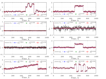
Figure 1: Actual states $x_{1}$, $x_{2}$, $x_{3}$, $x_{4}$, $x_{5}$ and its estimates, as well as unknown inputs $d_{1}$, $d_{2}$ and $d_{3}$ and its estimates.

Figure 2: Trace of estimate error covariance of states, tr($P^{x}$), and unknown inputs, tr($P^{d}$).

Figure 1 shows a comparison of the input and state estimation of the first three MVU estimators for the first system with $H^{1}$. In this case, these estimators were successful at estimating the states as well as the unknown inputs. It does appear from Figure 2 all three estimators produces the same steady-state error covariances. However, if we consider the results of all six systems in Table 1, we observe that PLISE is outperformed by CYWZ and ULISE. Note also that ULISE are consistently the best filters, which agrees with the claim in Section 5.4 of being globally optimal over the class of all linear unbiased state and input estimates for systems with unknown inputs, while CYWZ performs just as well, which shows that in this particular example, the replacement of the generalized least squares estimate of $d_{2,k}$ with the ordinary least squares estimate have little impact on the filter performance.

Table 1: Steady-state Performance of CYWZ, ULISE, PLISE, GDM, FSY and YZF.

		$P^{x}_{11}$	$P^{x}_{22}$	$P^{x}_{33}$	$P^{x}_{44}$	$P^{x}_{55}$	$P^{d}_{11}$	$P^{d}_{22}$	$P^{d}_{33}$
$H^{1}$	CYWZ	0.1843	0.0091	0.0002	0.0004	0.0001	0.0099	0.0102	0.1923
	ULISE	0.1843	0.0091	0.0002	0.0004	0.0001	0.0099	0.0102	0.1923
	PLISE	0.1843	0.0091	0.0002	0.0004	0.0001	0.0099	0.0102	0.1923
	GDM	N/A	N/A	N/A	N/A	N/A	N/A	N/A	N/A
	FSY	N/A	N/A	N/A	N/A	N/A	N/A	N/A	N/A
	YZF	N/A	N/A	N/A	N/A	N/A	N/A	N/A	N/A
$H^{2}$	CYWZ	0.1494	0.0052	0.0002	0.0004	0.0001	0.0097	0.0102	0.1574
	ULISE	0.1494	0.0052	0.0002	0.0004	0.0001	0.0097	0.0102	0.1574
	PLISE	0.1614	0.0053	0.0002	0.0004	0.0001	0.0102	0.0102	0.1889
	GDM	0.1494	0.0052	0.0002	0.0004	0.0001	0.0097	0.0102	0.1574
	FSY	0.1724	0.0108	0.0002	0.0004	0.0001	0.0097	0.0102	0.1648
	YZF	0.1494	0.0052	0.0002	0.0004	0.0001	0.0097	0.0102	0.1574
$H^{3}$	CYWZ	0.0076	0.0052	0.0002	0.0004	0.0001	0.0097	0.0102	0.3906
	ULISE	0.0076	0.0052	0.0002	0.0004	0.0001	0.0097	0.0102	0.3906
	PLISE	0.0076	0.0053	0.0002	0.0004	0.0001	0.0102	0.0102	0.3961
	GDM	N/A	N/A	N/A	N/A	N/A	N/A	N/A	N/A
	FSY	N/A	N/A	N/A	N/A	N/A	N/A	N/A	N/A
	YZF	N/A	N/A	N/A	N/A	N/A	N/A	N/A	N/A
$H^{4}$	CYWZ	0.0076	0.0257	0.0002	0.0004	0.0001	0.0348	0.0102	0.4925
	ULISE	0.0076	0.0257	0.0002	0.0004	0.0001	0.0348	0.0102	0.4925
	PLISE	0.0076	0.0258	0.0002	0.0004	0.0001	0.0349	0.0102	0.4925
	GDM	N/A	N/A	N/A	N/A	N/A	N/A	N/A	N/A
	FSY	N/A	N/A	N/A	N/A	N/A	N/A	N/A	N/A
	YZF	N/A	N/A	N/A	N/A	N/A	N/A	N/A	N/A
$H^{5}$	CYWZ	0.0079	0.0074	0.0002	0.0004	0.0001	0.0089	0.0102	0.0099
	ULISE	0.0079	0.0074	0.0002	0.0004	0.0001	0.0089	0.0102	0.0099
	PLISE	0.0079	0.0074	0.0002	0.0004	0.0001	0.0089	0.0102	0.0150
	GDM	N/A	N/A	N/A	N/A	N/A	N/A	N/A	N/A
	FSY	N/A	N/A	N/A	N/A	N/A	N/A	N/A	N/A
	YZF	N/A	N/A	N/A	N/A	N/A	N/A	N/A	N/A
$H^{6}$	CYWZ	0.0076	0.0218	0.0002	0.0004	0.0001	0.0309	0.0102	0.0097
	ULISE	0.0076	0.0218	0.0002	0.0004	0.0001	0.0309	0.0102	0.0097
	PLISE	0.0078	0.0257	0.0002	0.0004	0.0001	0.0368	0.0102	0.0165
	GDM	0.0076	0.0218	0.0002	0.0004	0.0001	0.0309	0.0102	0.0097
	FSY	0.0315	0.0232	0.0002	0.0004	0.0001	0.0310	0.0102	0.0100
	YZF	0.0076	0.0218	0.0002	0.0004	0.0001	0.0309	0.0102	0.0097

On the other hand, when the direct feedthrough matrix has full rank, as with $H^{2}$ and $H^{6}$, GDM and YZF performed just as well as CYWZ and ULISE, which is consistent with the claim of global optimality of GDM in Hsieh.2010 . In both examples, the intentionally suboptimal FSY filter performs better than PLISE at estimating the unknown inputs, but is worse than PLISE when estimating the system states.

7.2 Multi-vehicle Tracking

In this second example, we consider the problem of the position and velocity tracking of multiple vehicles, for e.g., at an intersection, with partial information about the decisions of the vehicles as well as faulty sensor readings. This can be particularly useful for the design of intelligent transportation systems. To simplify the problem, we consider the scenario with two vehicles, in which each vehicle only has access to its own control input, thus, the input of the other vehicle is unknown. Furthermore, the velocity measurement of the vehicle is corrupted by a time-varying bias, which is also unknown. Thus, we model the linear continuous-time model of the coupled system as:

$$\begin{bmatrix}\dot{p}\\ \ddot{p}\\ \dot{q}\\ \ddot{q}\end{bmatrix} =\begin{bmatrix}0&1&0&0\\ 0&-0.1&0&0\\ 0&0&0&1\\ 0&0&0&-0.1\end{bmatrix}\begin{bmatrix}p\\ \dot{p}\\ q\\ \dot{q}\end{bmatrix}+\begin{bmatrix}0\\ 0\\ 0\\ 1\end{bmatrix}u+\begin{bmatrix}0&0\\ 1&0\\ 0&0\\ 0&0\end{bmatrix}\begin{bmatrix}d_{1}\\ d_{2}\end{bmatrix}+\begin{bmatrix}0\\ w_{1}\\ 0\\ w_{2}\end{bmatrix}$$

$$y =\begin{bmatrix}1&0&0&0\\ 0&1&0&-1\\ 0&0&1&0\\ 0&0&0&1\end{bmatrix}\begin{bmatrix}p\\ \dot{p}\\ q\\ \dot{q}\end{bmatrix}+\begin{bmatrix}0&0\\ 0&0\\ 0&0\\ 0&1\end{bmatrix}\begin{bmatrix}d_{1}\\ d_{2}\end{bmatrix}+v$$

where $p$ and $\dot{p}$, and $q$ and $\dot{q}$, are the displacements and velocities of the uncontrolled and controlled vehicle, respectively. $d_{1}$ is the unknown input of the uncontrolled vehicle while $d_{2}$ represents the unknown time-varying bias. The intensities of the zero mean, white Gaussian noises, $w=\begin{bmatrix}0&w_{1}&0&w_{2}\end{bmatrix}^{\top}$ and $v$, are given by:

$$Q_{c} =10^{-4}\begin{bmatrix}0&0&0&0\\ 0&1.6&0&0\\ 0&0&0&0\\ 0&0&0&0.9\end{bmatrix};\ R_{c}=10^{-4}\begin{bmatrix}1&0&0&0\\ 0&0.16&0&0\\ 0&0&0.9&0\\ 0&0&0&2.5\end{bmatrix}.$$

Since the proposed filter is for discrete systems, we first convert the continuous dynamics to a discrete equivalent model with sample time $\triangle t=0.01s$, assuming zero-order hold for the known and unknown inputs, $u$ and $d$:

$$x_{k+1} =A_{d}x_{k}+B_{d}u_{k}+G_{d}d_{k}+w_{d,k}$$

$$y_{k} =C_{d}x_{k}+H_{d}d_{k}+v_{d,k}$$

where $x=\begin{bmatrix}p&\dot{p}&q&\dot{q}\end{bmatrix}^{\top}$, $k=0,1,2,\ldots$ and $t=k\triangle t$, while the system matrices as well as noise covariances can be computed, e.g., using conversion algorithms involving matrix exponentials as in DeCarlo.1989 ; VanLoan.1978 , to obtain:

$$A_{d} =\begin{bmatrix}1&0.01&0&0\\ 0&-0.999&0&0\\ 0&0&1&0.01\\ 0&0&0&0.999\end{bmatrix};\ B_{d}=\begin{bmatrix}0\\ 0\\ 0\\ 0.01\end{bmatrix};$$

$$C_{d} =\begin{bmatrix}1&0&0&0\\ 0&1&0&-1\\ 0&0&1&0\\ 0&0&0&1\end{bmatrix};\ G_{d}=\begin{bmatrix}0&0\\ 0.01&0\\ 0&0\\ 0&0\end{bmatrix};\quad H_{d}=\begin{bmatrix}0&0\\ 0&0\\ 0&0\\ 0&1\end{bmatrix};$$

$$Q_{d} =10^{-5}\begin{bmatrix}0.0000&0.0008&0&0\\ 0.0008&0.1598&0&0\\ 0&0&0.0000&0.0004\\ 0&0&0.0004&0.0899\end{bmatrix};\;R_{d}=R_{c},$$

with $d_{1,k}$ and $d_{2,k}$ as shown in Figure 3 (where $t=k\Delta t$).

From Figure 3, we observe that both variants of the filter proposed in this paper successfully estimate the system states and the unknown inputs, which consist of the input of the uncontrolled vehicle and the time-varying measurement bias. The slight difference between the two variants can be seen in Figure 4 where the rate of convergence of trace of the unknown input estimate error covariance of the PLISE variant is slightly slower.

Figure 3: Actual states $x_{1}$, $x_{2}$, $x_{3}$, $x_{4}$ and its estimates, as well as unknown inputs $d_{1}$, $d_{2}$, and its estimates.

Figure 4: Trace of estimate error covariance of states, tr($P^{x}$), and unknown inputs, tr($P^{d}$) for the first $0.25s$.

8 Conclusion

This paper presented a unified filter for simultaneously estimating the states and unknown inputs in an unbiased minimum-variance sense for linear discrete-time stochastic systems, without any restriction on the direct feedthrough matrix of the system. Two variants of the filter is proposed, one of which uses the propagated state estimate for unknown input estimation (PLISE), and the other with the updated state estimate (ULISE). We proved that ULISE is also globally optimal over the class of all linear unbiased state and input estimates for systems with unknown inputs and provided stability conditions for the filter, which are shown to be closely related to the strong detectability of the system. Simulation results have shown that ULISE was the best estimator in all the test trials, whereas PLISE, though is not globally optimal, performed reasonably well.

A possible future direction is the extension of the current unified filter to linear continuous-time systems, switched systems and nonlinear systems.

References

- [1] R. Verma and D. Del Vecchio. Semiautonomous multivehicle safety. IEEE Robotics Automation Magazine, 18(3):44–54, Sept. 2011.
- [2] P. K. Kitanidis. Unbiased minimum-variance linear state estimation. Automatica, 23(6):775–778, November 1987.
- [3] R. Patton, R. Clark, and P.M. Frank. Fault diagnosis in dynamic systems: theory and applications. Prentice-Hall international series in systems and control engineering. Prentice Hall, 1989.
- [4] G. De Nicolao, G. Sparacino, and C. Cobelli. Nonparametric input estimation in physiological systems: Problems, methods, and case studies. Automatica, 33(5):851 – 870, 1997.
- [5] M. Darouach and M. Zasadzinski. Unbiased minimum variance estimation for systems with unknown exogenous inputs. Automatica, 33(4):717–719, 1997.
- [6] M Hou and RJ Patton. Optimal filtering for systems with unknown inputs. IEEE Transactions on Automatic Control, 43(3):445–449, 1998.
- [7] M. Darouach, M. Zasadzinski, and M. Boutayeb. Extension of minimum variance estimation for systems with unknown inputs. Automatica, 39(5):867 – 876, 2003.
- [8] Y. Cheng, H. Ye, Y. Wang, and D. Zhou. Unbiased minimum-variance state estimation for linear systems with unknown input. Automatica, 45(2):485–491, 2009.
- [9] D. Simon. Optimal state estimation: Kalman, , and nonlinear approaches. John Wiley & Sons, 2006.
- [10] Z. Wang, Y. Liu, and X. Liu. filtering for uncertain stochastic time-delay systems with sector-bounded nonlinearities. Automatica, 44(5):1268 – 1277, 2008.
- [11] Z. Wang, H. Dong, B. Shen, and H. Gao. Finite-horizon filtering with missing measurements and quantization effects. IEEE Transactions on Automatic Control, 58(7):1707–1718, July 2013.
- [12] X. Li and H. Gao. Robust finite frequency filtering for uncertain 2-D systems: The FM model case. Automatica, 49(8):2446 – 2452, 2013.
- [13] H. J. Palanthandalam-Madapusi and D. S. Bernstein. Unbiased minimum-variance filtering for input reconstruction. In American Control Conference, pages 5712–5717, 2007.
- [14] C. Hsieh. Robust two-stage Kalman filters for systems with unknown inputs. IEEE Transactions on Automatic Control, 45(12):2374–2378, December 2000.
- [15] S. Gillijns and B. De Moor. Unbiased minimum-variance input and state estimation for linear discrete-time systems. Automatica, 43(1):111–116, January 2007.
- [16] S. Gillijns and B. De Moor. Unbiased minimum-variance input and state estimation for linear discrete-time systems with direct feedthrough. Automatica, 43(5):934 – 937, March 2007.
- [17] H. Fang, Y. Shi, and J. Yi. On stable simultaneous input and state estimation for discrete-time linear systems. International Journal of Adaptive Control and Signal Processing, 25(8):671–686, 2011.
- [18] S.Z. Yong, M. Zhu, and E. Frazzoli. Simultaneous input and state estimation for linear discrete-time stochastic systems with direct feedthrough. In IEEE Conference on Decision and Control, pages 7034–7039, Dec 2013.
- [19] C. Hsieh. Extension of unbiased minimum-variance input and state estimation for systems with unknown inputs. Automatica, 45(9):2149 – 2153, 2009.
- [20] H. Fang, Y. Shi, and J. Yi. On stable simultaneous input and state estimation for discrete-time linear systems. International Journal of Adaptive Control and Signal Processing, 25(8):671–686, 2011.
- [21] M.L.J. Hautus. Strong detectability and observers. Linear Algebra and its Applications, 50:353 – 368, 1983.
- [22] N Suda and E Mutsuyoshi. Invariant zeros and input-output structure of linear, time-invariant systems. International Journal of Control, 28(4):525–535, 1978.
- [23] W. S. Kerwin and J. L. Prince. On the optimality of recursive unbiased state estimation with unknown inputs. Automatica, 36(9):1381 – 1383, 2000.
- [24] L. M. Silverman. Discrete Riccati equations: Alternative algorithms, asymptotic properties, and system theory interpretations, volume 12 of Control and Dynamic Systems. Academic Press, 1976.
- [25] A.H. Sayed. Fundamentals of Adaptive Filtering. Wiley, 2003.
- [26] B.D.O. Anderson and John B. Moore. Detectability and stabilizability of time-varying discrete-time linear systems. SIAM Journal on Control and Optimization, 19(1):20–32, 1981.
- [27] M. A. Peters and P. A. Iglesias. A spectral test for observability and reachability of time-varying systems. SIAM Journal on Control Optimization, 37(5):1330–1345, August 1999.
- [28] D.S. Bernstein. Matrix Mathematics: Theory, Facts, and Formulas (Second Edition). Princeton reference. Princeton University Press, 2009.
- [29] N. R. Draper and H. Smith. Applied Regression Analysis (Wiley Series in Probability and Statistics). Wiley-Interscience, third edition, April 1998.
- [30] R.E. Kalman. A new approach to linear filtering and prediction problems. Transactions of the ASME–Journal of Basic Engineering, 82(Series D):35–45, 1960.
- [31] S. Chan, G. Goodwin, and K. Sin. Convergence properties of the Riccati difference equation in optimal filtering of nonstabilizable systems. Automatic Control, IEEE Transactions on, 29(2):110–118, February 1984.
- [32] C. de Souza, M. Gevers, and G. Goodwin. Riccati equations in optimal filtering of nonstabilizable systems having singular state transition matrices. IEEE Transactions on Automatic Control, 31(9):831–838, September 1986.
- [33] J.Y. Keller, L. Summerer, M. Boutayeb, and M. Darouach. Generalized likelihood ratio approach for fault detection in linear dynamic stochastic systems with unknown inputs. Intern. Journal of Systems Science, 27(12):1231–1241, 1996.
- [34] C. Hsieh. On the global optimality of unbiased minimum-variance state estimation for systems with unknown inputs. Automatica, 46(4):708 – 715, 2010.
- [35] R. A. DeCarlo. Linear systems: a state variable approach with numerical implementation. Prentice-Hall, Inc., Upper Saddle River, NJ, USA, 1989.
- [36] C. Van Loan. Computing integrals involving the matrix exponential. IEEE Transactions on Automatic Control, 23(3):395–404, 1978.