Quantized Faraday effect in (3+1)-dimensional and (2+1)-dimensional
systems
L. Cruz Rodríguez
lcruz@fisica.uh.cuDepartamento de Física General, Facultad de Física, Universidad de la Habana, San Lázaro y L, Vedado La Habana, 10400, Cuba
A. Pérez Martínez
aurora@icimaf.cuInstituto de Cibernética Matemática y Física (ICIMAF)
Calle E esq 15 No. 309 Vedado, La Habana, 10400, Cuba
H. Pérez Rojas
hugo@icimaf.cuInstituto de Cibernética Matemática y Física (ICIMAF)
Calle E esq 15 No. 309 Vedado, La Habana, 10400, Cuba
E. Rodríguez Querts
elizabeth@icimaf.cuInstituto de Cibernética Matemática y Física (ICIMAF)
Calle E esq 15 No. 309 Vedado, La Habana, 10400, Cuba
Abstract
We study Faraday rotation in the quantum relativistic
limit. Starting from the photon self-energy in the presence of a constant magnetic
field the rotation of the polarization vector of a plane electromagnetic wave which travel
along the fermion-antifermion gas is studied. The connection between Faraday Effect and Quantum Hall Effect
(QHE) is discussed.
The Faraday Effect is also investigated for a massless relativistic
(2D+1)-dimensional fermion system which is derived by using the
compactification along the dimension parallel to the magnetic field.
The Faraday angle shows a quantized behavior as Hall conductivity in
two and three dimensions.
I Introduction
Plane-polarized light penetrating in a magnetized transparent
charged medium and moving parallel to the magnetic field B
rotates its plane of polarization as a consequence of
birefringence: the incoming wave splits in two opposite circularly
polarized modes moving with different speeds (and frequencies), and
the polarization vector rotates. This is the Faraday effect
Faraday .
Faraday rotation (FR) is clearly manifest for photon propagation
parallel to the magnetic field. The symmetry properties behind
theFaraday effect are the following: the field B (which we
take along the axis), breaks the Lorentz symmetry group in two
subgroups, the translations along (leading to the
conservation of momentum component ), and the rotations around
(leading to the conservation of angular momentum ). The
generator of rotations around is the antisymmetric matrix
whose eigenvectors are
proportional to the complex unit vectors
,
where are related respectively to positive and
negative circular polarizations. If the system is invariant,
both opposite circular polarizations contribute symmetrically,
leading to equal speeds of light propagating along B. If
the system is noninvariant under , the speeds of light differ for
opposite circular polarizations. The resulting polarization vector
rotates describing a circumference (in general an ellipse), and the
Faraday effect arises.
For propagation perpendicular to B, two elliptically polarized modes arise, one of their semiaxes being along the propagation vector , the rotation being in the plane orthogonal to B containing k1 -Elizabeth .
The FR is indeed a particular case of the general problem of photon
propagation in a charged medium hugo1982 . In nonrelativistic
media, like the ionosphere and insulators it is a well-known
phenomena where the classical and semiclassical approaches can be
applied successfully Faraday .
However, FR effects have been also observed in electromagnetic waves
coming from astrophysical objects Olivo1-6 . Some of these
sources are compact objects which are characterized by high
densities and strong magnetic fields that can reach up to
G in magnetars Duncan:2000pj . Hence the physical process
involved in the case of compact objects requires an adequate
treatment from the point of view of a quantum-relativistic approach.
On the other hand, in quasiplanar condensed matter systems such as
graphene (a genuine monolayer of carbon atoms in a honeycomb array,
whose theoretical properties are essentially described by a
two-dimensional relativistic chiral fermion system
NovoselovNature2005 -aurora ), FR is observed when
light propagates perpendicular to the graphene layer in the presence
of a static magnetic field with and
the relation between the Faraday angle and the nonstatic
() Hall conductivity has been pointed out
japoneses -castro .
From the point of view of novel applications of graphene,
magneto-optical phenomena such as Faraday effect must be understood
from both the theoretical and experimental points of view.
Theoretical studies of the conductivity tensor in the static limit
aurora , Gusyin and nonstatic regime have been done
gusynin2009 -gusyninnewjournal . Recently, FR has been
detected in single-layer and multilayered epitaxial graphene
experimental . The measurements report a giant value of the
rotation angle which comes exclusively from the graphene system (the
substrate did not show any FR).
In spite of the differences in contexts, the description of the
Faraday effect in both, the astrophysical and graphene scenarios,
can be theoretically tackled by considering photon propagation
parallel to the constant magnetic field in quantum-relativistic
dense matter.
The scope of the present paper is to describe the FR effect and to
obtain the Faraday angle for (3+1)-dimensional (3D+1) and 2+1
dimensional (2D+1) systems, starting from the same formalism: the
relativistic conductivity tensor in 3D+1 for a massive fermion
system. Our goal will be to show the connection between Hall
conductivity and the Faraday effect and the quantization of the
Faraday angle Volkov .
In a previous paper aurora , the Hall conductivity for a
massless relativistic fermion system was studied by starting from
the quantum-relativistic photon self-energy tensor in the QED
framework using the approach of Ref. aurora90 to obtain the
static limit. Now, as we are interested in FR, this problem should
be generalized to the nonstatic limit ().
In Ref. hugo1982 a detailed study of the structure of the
photon self-energy in the presence of a magnetic field at finite
density and temperature was done. Photon self-energy satisfies
properties of gauge and Lorentz and CPT invariance. General
properties of the photon self-energy and the dispersion equations
for photons propagating in the medium were solved in two cases:
photon propagating parallel and perpendicular to the magnetic field
hugo1982 .
In this paper we focus on the propagation parallel to the magnetic
field which establishes a relation between the Hall and Faraday
effects, so we take advantage of these calculations. We have also
particularized the study to 2D+1 with the aim to describe
graphene-like systems.
Our calculations have been done in the imaginary-time formalism. For
and systems we have obtained the FR angle that
the light undergoes upon propagating in a dense fermion system where the
chemical potential is greater than temperature ().
The weak-field limit for light propagating in a magnetized plasma
was studied in Avjit , taking the dependence of the
self-energy with regard to B in a linear approximation. In
Ref. olivo a calculation of the photon self-energy is made
for strong and moderate fields but . In both papers the
Faraday effect is considered in some particular cases and the
semiclassical results have been reproduced. The real-time formalism
was used in Refs. Avjit -olivo .
Our findings are relevant for two main reasons: first, we have
extended them to the nonstatic limit from previous calculation
aurora90 -aurora of 3D+1 relativistic massive fermions
and 2D+1 relativistic massless Hall and Ohm conductivities. Second,
we have found the connection between FR angle and Hall conductivity
(the Faraday angle depends on the admittivity: complex conductivity,
but the leading term is proportional to the Hall conductivity). This
result for 3D+1 and 2D+1 systems shows that it is a consequence of
general properties of QED in external magnetic fields at finite
density. The angle as a function of the photon frequency
has branching points for 3D+1 relativistic dense massive fermion
systems as well as for 2D+1 massless systems a discrete set of
values. Hence, FR shows the effect of quantization of the
quantum Hall effect at nonzero frequency. Our results for 2D+1
massless system are in agreement with previous theoretical work
for FR in graphene reported in Refs. Tan -castro . The
2D+1 results have been obtained from 3D+1 results by dimensional
compactification.
Astrophysical applications of our findings on FR angle can be
expected in the context of radiation propagating through neutron
stars magnetospheres. This problem will be discussed in a
forthcoming presentation.
The paper is organized as follows: In Sec. II we start from
the one-loop approximation of the photon self-energy in the
presence of a constant and uniform magnetic field and obtain the
relativistic Hall and Ohm conductivities in the nonstatic
approximation by generalizing the results obtained in Ref.
aurora90 . In Sec. III the 3D+1 Faraday effect is
discussed and the Faraday angle is obtained to first order as half
of the Hall conductivity. Then, the 2D+1 massless QED limit is
obtained, and the expression for the Hall and Ohm conductivities are
written in Sec. IV. In Sec. V the Faraday effect
and angle are discussed in 2D+1 dimensions obtaining the same
dependence with regard to the Hall conductivity as the 3D+1 case in
the first-order approximation. Finally, in Sec. VI we state
the concluding remarks. Appendices show the calculations relevant to
our results.
II Photon self-energy in presence of magnetic field
The photon self-energy in quantum electrodynamics in an
external magnetic field was calculated at finite temperature and nonzero density in Ref. 1 .
The total electromagnetic field is written where refers to the
external magnetic field and to the radiation field. The photon self-energy (also called the
polarization operator), can also be interpreted as the linear-term coefficient of the functional expansion of the four-current in powers of the electromagnetic field . That is, .
The introduction of a chemical potential is associated with a non-neutral electron-positron charged medium.
The system is thus assumed as noninvariant, and total charge neutrality is guaranteed by the
assumption of a hadron background. This background, however, is not taken into account in any of the further calculations.
The generalized Furry’s theorem Fradkin establishes that odd
powers of will be associated with odd powers of through
antisymmetric tensor structures. That is, the self-energy contains antisymmetric odd-in- terms. Also,
as gauge invariance is satisfied, it implies that the self-energy tensor satisfies the four-dimensional gauge invariance condition
.
We have for the photon self-energy the expression111Unless specified otherwise, we use natural units .
(1)
For the calculation of the components of we take (1) in the
one loop approximation with the temperature Green’s functions being the solution
of the Dirac equation in a constant magnetic field B such that ,
directed along the -axis
(2)
where , and is the
chemical potential for the electron-positron gas. It is also
important to remark that Eq. (2) defines the fermion temperature-dependent Green’s
function for in the interval to ; .
In the one-loop approximation the Fourier transform of the
polarization tensor has the form
(3)
where and runs over integers from to
.
Substituting the expression of the Green function of fermions we obtain
the self-energy tensor as
(4)
where , , n and are the Landau numbers and in what follows we will use the notation and
Let us remark that the presence of the magnetic field in the
direction breaks the spatial symmetry, hence
in Eq. (4) only the integral over has survived. The integral over where
As mention earlier, in Ref. hugo1982 the structure of
self-energy of the photon (4) in presence of a
magnetic field at finite density and temperature was obtained by
considering the properties of gauge and Lorentz invariance and
invariance. Six independent transverse tensors can be built in
terms of the four vectors: the momentum of the photon , the
product of the external electromagnetic field tensor
and its square by , leading respectively as
and , and the
four-velocity of the medium (a summary of these properties
can be found in the appendix). As our goal is to study the Faraday
effect in connection to the conductivity tensor we will concentrate
on the case of a photon propagating parallel to the magnetic field
hugo1982 ; in that case only three scalars are
independent. As we will show in the next sections only two of them
are related to the conductivity and also to Faraday effect.
Relativistic Hall and Ohm conductivity in non-static limit ()
This section is devoted to studying the 3D+1 relativistic Hall and
Ohm conductivities in the nonstatic limit (). The
expression for the spatial part of the current density is linear in
terms of the perturbative magnetic field and is given in terms of
the photon self-energy of the medium by aurora90
(5)
where and , having in mind the transversality
condition given by , due to gauge invariance, Eq. (5) can be written as
(6)
where is the admittivity (complex conductivity tensor) and is
the electric field.
We will be especially interested in the real conductivity
. The contribution to the current
density in Eq. (6) due to
can be written as
(7)
where
and
is a pseudovector
associated with
. and are, respectively, the
antisymmetric and symmetric parts of the polarization tensor
aurora and aurora90 .
In the particular case where the electric field is the polarization
vector of a transverse wave propagating along the magnetic field B,
being , the conductivity tensor can be written in the following
way:
(8)
where is the antisymmetric unity tensor,
and
(9)
(10)
where the scalar quantities and depend on the
frequency- , the momentum and also the temperature,
chemical potential and magnetic field hugo1982 . From Eq.
(8) we can identify ,
with the Ohm and Hall conductivities respectively. The scalar
can be written as
(11)
and is the integral
(12)
(13)
for , ,
are the Fermi-Dirac distribution
for fermions and antifermions, respectively.
The scalar is
(14)
where and
(15)
and
Thus, we have the expressions for the scalars r and t in the one
loop approximation for the fermion-antifermion gas, with the
assumption of . Now, starting from them we can study
the Hall and Ohm conductivities in some particular limits which are
relevant for applications in astrophysics as well as in
graphene-like systems.
II.1 3D+1 Hall conductivity
The Hall and Ohm conductivities Eqs. (9) and (10)
are given as imaginary parts of the scalars and
respectively. At frequencies different from zero the integrals
(12) and (15) have singularities which come
from the zeros of the denominator . But the Hall conductivity is
the imaginary part of , thus the contribution to the Hall
conductivity comes from the real part of , which means to
consider the principal value of the integral [see the appendix,
first term of (102)]. The result is the following:
(16)
where
(17)
The denominator in (17) can be written as
, where are the
roots of the equation (see details in hugo1982 )
(18)
and
(19)
and we have for
(20)
In the degenerate limit where and are replaced by
a step functions , , after integration we obtain
(21)
where is the Fermi momentum.
As are given by Kronecker
expressions and taking the long wave limit we
have for the expression
(22)
where .
From Eq. (17) at zero frequency (static limit)
we recover the quantum Hall conductivity obtained in Ref.
aurora90 :222we have returned to the units and
for obtain this result.
(23)
The sum over Landau levels is up to the integer number
, .
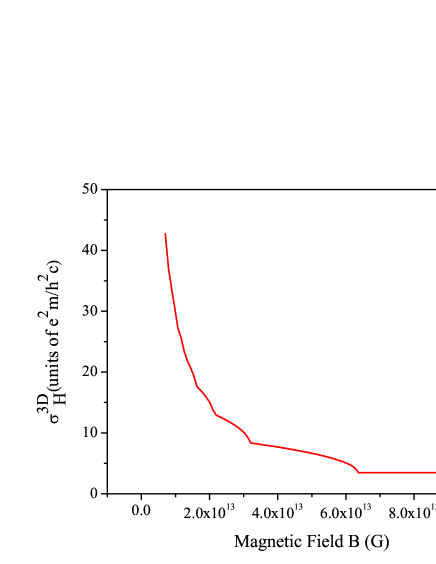
In Fig. 1, the three-dimensional (3D) nonstatic
Hall conductivity is plotted for constant chemical potential and
frequency as a function of the magnetic field. The curved step
behavior is illustrated; this behavior is also observed in the
static limit aurora90 .
Figure 1: (Color online)3D Hall conductivity as a function of the magnetic field,
where B runs between and G and MeV.
II.2 3D+1 Ohm conductivity
Our aim now is to calculate the Ohm conductivity given by Eq.
(9). A detailed calculation of can be found in
hugo1982 . It expression comes from the imaginary part of the
integral (15), which is related to the singularities
due to absorptive process, and it can be written in two different
cases, the first one, where , and absorption is
only due to excitation of particles, and a second one, where
and absorption is due to excitation and also
pair creation. In the present study we are going to use the
expression of in the region of because
we will take the long wavelength limit ().
Furthermore, only the region of real frequencies, which means,
is considered. To find the imaginary part
of the formulas (101)-(105) will be
used, after that we have the Ohm conductivity as
(24)
where
(25)
Equation (24) is written for ,
where and are the
values of the energy at the branching points for the excitation and
pair creation absorption processes respectively,
(26)
The step function over in Eq.
(24) defines the regions where excitation and pair
creation take place, where and
are the branching points located
at plane
(27)
Now, our attention is focused in the long wavelength and degenerate limit, in order to get a better
understanding of our results, we separate them for each region.
a) Region I: excitation case.
In this region absorption occurs due to only the excitation of particles to higher energy levels.
As , then .
The solution for the energy are: . In order to
have positive energies, which could be important in the degenerate limit, the sum is restricted to . Also, the condition , in this limit, implies .
Finally, considering the degenerate limit, the Ohm conductivity in I is given by
(28)
The sum over the integer goes to determined by the
restriction imposed by Eq. (27). The combination of
the degenerate functions tells us that the Ohm conductivity does not
vanish if
b)Region II: pair creation.
In this region absorption may be due to excitation and also to pair creation. The
corresponding solution for the energies are: .
In this case there is no restriction for the sum over n, and the
condition , implies . Then, the expression
for the Ohm conductivity in the degenerate limit in II is
(29)
and from the degenerate distribution, we obtained that the
Ohm conductivity does not vanish if
(30)
Let us remark that in the static limit, the Ohm
conductivity is zero as was checked in Ref. aurora90 .
III Quantum Faraday Effect for a relativistic fermion gas
Photons propagating in a relativistic fermion-antifermion
() medium at zero temperature and nonzero
particle density (chemical potential ) is of special interest
for astrophysics. The one-loop diagram describing the process
accounting for the photon self-energy interaction contains, in
addition to the virtual creation and annihilation of the pair, the
process of absorption and subsequent emission of one photon by the
fermions and/or antifermions.
The propagation of an electromagnetic wave in the medium can be
described by the Maxwell equations
(31)
which could be written in momentum space as
(32)
We will consider in what follows that the photon propagates parallel to the magnetic field.
As in Sec. II, is the self-energy of the
photon propagating in a magnetized dense medium, so it depends on
, , and magnetic field, apart from and .
To solve the dispersion relation (32) we need to diagonalize . The
general covariant structure of the photon self-energy leads to the following
expression:
(33)
where and are the
eigenvalues and the eigenvectors of , respectively,
which satisfies the secular equation
(34)
In the particular case of propagation along the magnetic field
there are three nonvanishing eigenvalues. The first
two are transverse modes hugo1982 -1 (see appendix for details).
(35)
with
(36)
which describe a circularly
polarized wave in the plane perpendicular to B with
different eigenvalues,
that is, opposite directions, which
is the key of the Faraday effect. Also, there is a third mode
corresponding to a longitudinal wave which propagates along the
magnetic field , and is the corresponding
eigenvalue.
Let us consider the propagation of an electromagnetic wave, which at
is linearly polarized along the axes. Note that,
because the system has rotational symmetry with regard to B
( ), we can choose the direction of the eigenvectors
arbitrarily orthogonal to B. We can then
set , and decompose
the wave into two circularly polarized waves
(39)
where are the solutions of the dispersion relations for the eigenmodes
(40)
In order to solve the dispersion relation, the complex functions and in (40) are considered in an approximation independent on (35).
The electric field associated with the wave is given by
(41)
where
are the polarization vectors of the left and right circularly
polarized waves, respectively. So, the superposition of both modes
leads to an elliptically polarized wave, whose principal axis
rotate.
The amount of the FR angle, after traveling a distance in the
medium, can be obtained from (see also Refs.
Avjit -olivo )
(42)
where are the refraction indices of the left- and right-circularly polarized waves, respectively, and can be defined as 1
(43)
Using , then the Faraday angle can be obtained directly from
Eqs. (41) and
(42):
(44)
where
(45)
If
we can roughly write
(46)
Furthermore, if also , in the
leading-order approximation
(47)
and, according to
the relation given in Ref. (44), we obtain for
the rotated Faraday angle per unit length 333We have returned
to the units and to obtain this result.
(48)
Equation (48) shows the relation between Faraday
angle and the Hall conductivity. Let us note that in general the
Faraday angle depends on the terms of the admittivity tensor but the
leading term comes from the Hall conductivity. This result obtained
for 3D+1 systems shows that it is a consequence of general
properties of QED in an external magnetic field at finite density.
In Sec. V we have obtained in 2D+1 limit. This result has been
obtained theoretically in 2D+1 systems Tan , rusos ,
japoneses1 .
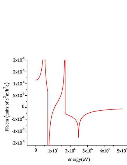
The Faraday angle in the degenerate limit( is given
by Eq. (22)) has been depicted in Fig.
2, for in a wide range of photon
energy. Because the Hall conductivity
(22) has two branching points for
, the curve has two peaks related to excitation
() and pair creation
(). Then a resonant behavior for the
Faraday angle is obtained, associated with both absorption processes
hugo1982 . Let us note that the Faraday angle should be a
finite value. The divergences are avoided if we use the solution of
the dispersion equation near the singular points.
The relativistic quantized medium makes the angle depend nonlinearly
on the magnetic field, contrary to the classical case of
interstellar medium where the relation with is linear and
depends on the electron density.
It is worthwhile to point out that Faraday effect is obtained as the
consequence of charge asymmetry of the system . When the
system has charge symmetry the scalar vanishes and the
Faraday effect is not manifested.
Figure 2: (Color online)Faraday angle per unit length as a function of energy, for MeV and G,
corresponding to . The curve was plotted in a wide range of the photon energy which includes the two branching points for the FR
IV Relativistic Hall and Ohm Conductivities in non-static limit (: 2D+1 system)
As is well known theoretically properties of
graphene are essentially described by Dirac massless fermions
(electrons) in two dimensions. This system is “relativistic” in the
sense that the spectra of electrons and holes can be mimicked as
two-dimensional relativistic chiral fermions where electrons and
holes move at velocities one hundredth the
speed of light NovoselovNature2005 . In this section with the
aim of studying a graphene like system we are going to obtain the 2D
Hall and Ohm conductivities in the nonstatic limit from the 3D
conductivities obtained in Sec. II. Two considerations can
be made: the first is to do a dimensional compactification
aurora ,aurora90 and the second one is to take the
limit aurora . To consider the first of our
assumptions, we assume that the fermion-antifermion gas is confined
to a box of length and the limit is
taken. Then the integral
over is replaced by a sum
over the integers .
Because and only the terms
remain in the sum. Then the 2D+1 limit is obtained taking
and and removing from all the expressions the
integrals . With this dimensional
reduction and the consideration of massless fermions in mind for
2D+1 Hall conductivity at
, we have ()
(49)
and
(50)
where . As in the earlier
section we consider the zero-temperature limit which means
substituting and zero
contribution of antifermions, since the gas is completely
degenerate. The Hall Conductivity has been written as
(51)
Let us remark that at we recover the expression of
quantum Hall Conductivity
.444we
have recovered the units and to write this result. The
Ohm conductivity should be obtained doing the dimensional reduction
in Eq. (15) considering massless fermions. In the
degenerate limit, we obtain
(52)
Let us note that in Eq. (52) the sum
over goes to .
Although our method of dimensional reduction described above is
valid for getting 2D+1 limits, it would be interesting to make a
full 2D+1 analysis of the problem by discussing the set of
independent tensor structures involved and their relation to the
obtained results. Reference Zeitlin is an early attempt to
deal with the 2D+1 case related to the Chern-Simons addition to the
Lagrangian.
To consider a graphene-like system in Eqs. (51) and
(52), additional considerations must
be taken into account. When the units and are recovered,
( is the Fermi velocity)aurora .
The expressions for the Hall and Ohm conductivities [Eqs.
51)-(52] must be multiplied
by two, to account for the sublattice-valley degeneracy in graphene.
The frequency must be substituted by where the imaginary part- is a
phenomenological parameter associated with system disorder
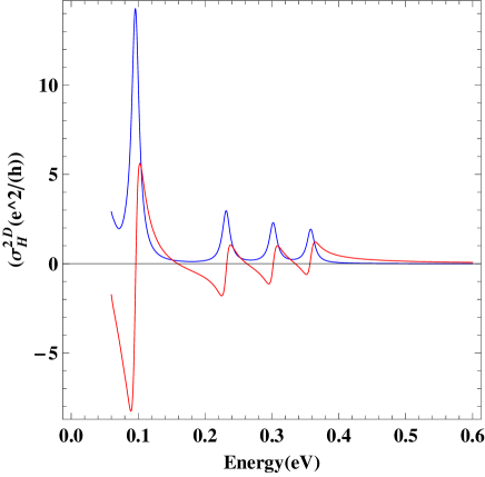
(rusos ,castro ). In Fig. 3 the 2D
Ohm conductivity is plotted as a function of energy for fixed
values of G, chemical potential MeV and
MeV, which are typical values for a graphene-like
system castro and rusos . The figure also shows the
imaginary part of the conductivity. Our results obtained with the
ansatz of a dimensional compactification are in
agreement with the theoretical studies of the Ohm conductivity in
graphene castro ,gusynin2009 .
Figure 3: (Color online)O
hm Conductivity (solid blue line) as a function of the photon energy for G, MeV and
MeV. We use cm/s. We also have plotted the imaginary part of the conductivity (dashed red line).
V 2D+1 system: Faraday effect and rotation Faraday angle
The purpose of this section is to study the Faraday
effect for a 2D+1 system (i.e., a graphene like system) starting
from the results obtained in Sec. III. Let us suppose that
the graphene plate is located at and the incoming
electromagnetic wave is linearly polarized along the
direction, and travels in the positive direction. Due to the
optical Faraday rotation of the polarization vector when the wave
crosses the graphene sheet, both the reflected and transmitted
component acquire a component along the direction
(rusos ,castro ,wallace ).
We can formally follow the procedure of by III by using the
solution of the dispersion relation for a photon in a stratified
medium, given by a 3D+1 relativistic electron-positron plasma,
situated between and , in vacuum.
To describe the propagation of an electromagnetic wave in the whole
space, let us start from the modified Maxwell Eq.
(31) as
(53)
where the -functions account for the inhomogeneity
in the Maxwell equation, which is only at . The boundary
conditions at the medium surfaces imply the continuity of the
electric field
(54)
and its
derivatives
(55)
If we consider an incident electromagnetic wave linearly polarized
along the direction,
(56)
the transmitted wave () can be written as
(57)
where are complex amplitudes and
correspond to the left- and right-polarized waves, respectively
Jackson . In order to express the amplitudes in
terms of the medium parameters and the amplitude of the incident
wave , we can follow the multiple-reflections method described
in Ref. MaxBorn . Let us define the complex total transmission
coefficients amplitudes
(58)
where the factors and come from the boundary
conditions (54) and
(55) and the exponentials
are related to the FR due to the propagation in the medium (as was
shown in detail in Sec. III). Because are complex
numbers, they can be written as , and using the definition given above for the Faraday angle [Eq.
44]
(59)
In the limit case , we can expand the exponentials
in (58) up to the linear term in , and obtain the approximate expressions
(60)
Finally, when ,
, where are the components of the 2D
complex conductivity tensor, obtained from the 3D
ones by the dimensional reduction prescription described in the previous
section. The Faraday angle in the 2D+1 limit is then given by
(61)
where and
(62)
It is easy to see from the last two equations that, in the leading
order approximation,
(63)
This relation between the Faraday angle and the Hall Conductivity
has been already obtained in graphene japoneses ,
rusos ,castro and here we have obtained it naturally
from the 3D result after a dimensional compactification.
It can be easily checked that our approach is equivalent to the one
followed in Ref. rusos by taking the limit
in Eq. (53).
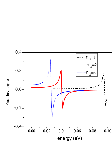
Figure 4: (Color online)
Faraday angle as a function of the energy for G, MeV and three different
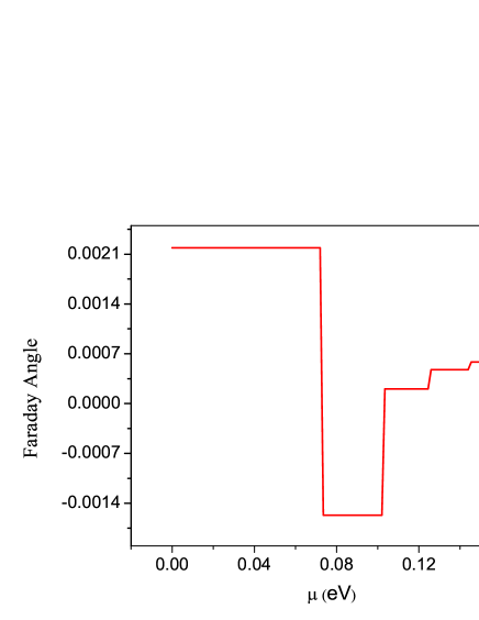
values of the chemical potential: MeVFigure 5: (Color online)
Faraday angle as a function of the chemical potential for G, MeV and
MeV. We use cm/s.
The Faraday angle is plotted in Figs.
(4) and (5) in
the degenerate limit [in which Hall conductivity is given by Eq.
(51)]. Figure (4) shows the
Faraday rotation angle versus for a fixed value of the
magnetic field G and maximum Landau numbers
, which corresponds to chemical potentials- MeV, respectively. Each curve shows peaks associated
with the poles of the Hall conductivity (51) showing a
resonant behavior for the Faraday angle when the frequency reaches
the values corresponding to the poles and absorption processes
occurs. The curves were done assuming MeV which is a
typical value of this quantity in graphene-like systems. The maximum
rotation angle for the parameters chosen is in agreement with the
angle predicted by Ref. Gusyin . In Fig.
5 the Faraday angle is plotted as a function
of chemical potential fixing G,
MeV and MeV. The curve shows a quantized behavior in
the same way as the Hall conductivity.
VI Conclusions
The study of propagation of an electromagnetic wave parallel to a
magnetic field has been done starting from quantum field theory
formalism at finite temperature and density. The quantum Faraday
effect has been studied in 3D+1 and 2D+1 systems. We have obtained
the relation between the FR angle and Hall Conductivity (the Faraday
angle is given by the complex conductivity, but the leading term
comes from the Hall conductivity). Our finding shows that it is a
consequence of general properties of propagation of an
electromagnetic wave parallel to a constant magnetic field, in a
quantum and relativistic dense system. We have found that Faraday
effect is consequence of the noninvariance of the system.
Due to the relation between Faraday effect and Hall conductivity we
started our calculations studying the conductivity tensor in
the nonstatic limit. Hall and Ohm conductivities have been
calculated in the limit of zero temperature relevant for
applications to astrophysical and graphene-like systems. The
calculations can be extended to the general case of finite
temperature.
Let us remark that in the present paper we have focused on the real
Ohm and Hall conductivities given by the imaginary part of and
the principal value of the integral , respectively. A more full
discussion of the complex conductivity including for instance the
imaginary part of integral (related to absorptive processes)
and the real part of will be discussed in a separate work.
The 2D+1 quantum relativistic system has also been studied by
introducing the ansatz of dimensional compactification of the
dimension, allowing us to obtain the Hall and Ohm conductivities in
the limit of zero temperature.
The Faraday angle shows a quantized behavior in both 3D+1 and 2D+1
relativistic system. The dependence of the Faraday angle with
frequency in graphene-like system is in agrement with theoretical
studies rusos -castro . Giant Faraday angles are found
for photon absorption frequencies. The outcome related to the
Faraday rotation angle in the astrophysical context, in particular
in the study of propagation of light in the magnetosphere of neutron
stars, deserves to be carefully analyzed. A separate study of this
topic will be addressed in a future work.
Acknowledgments
The authors thanks to A. Cabo and A. Gonzalez Garcia for fruitful discussions. This work has been supported under the grant CB0407 and the ICTP Office of External Activities through NET-35.
Appendix A Properties of the photon self-energy tensor
As a starting point we summarize some of the main features related
with the photon self-energy of an electron-positron plasma in
the presence of a constant magnetic field in the case of nonzero
temperature and nonvanishing chemical potential.
Under these conditions the polarization tensor may be expanded in
terms of six independent transverse tensors hugo1982 . As is shown in Ref. 1 ,
symmetric properties in quantum statistics, corresponding to generalization of the Onsager relations, reduce
the number of the basic tensors from 9 to 6:
(64)
The basic tensors are
(65)
(66)
(67)
where is the metric tensor and
is the dual of the electromagnetic tensor
.
These tensors are symmetric in the indexes , while the
following ones are antisymmetric
(68)
(69)
We introduce a set of orthonormal vectors which are the
eigenvectors of in the limit and
(70)
(71)
(72)
(73)
In the reference system in which the electron positron plasma is at
rest, the vectors look like
(74)
(75)
(76)
(77)
Using these vectors we can derive the scalars
(78)
(79)
(80)
(81)
and the pseudoscalar
(82)
(83)
In terms of this quantities the scalars in Eq.
64 may be written in
the rest frame as
(84)
(85)
(86)
(87)
(88)
The above expression were written taking into account that the
magnetic field is directed along the axis. Then,
can be expressed in terms of the base vectors
:
(89)
(90)
(91)
(92)
Finally the polarization tensor can be expressed in the
base as
(93)
From these results the eigenvalues could be determined by finding
the modes of the wave propagating in the medium. In the case of
propagation along the magnetic field, , we obtain
and and Eq. (93) becomes
(94)
with the eigenmodes and and eigenvalues
and . Equation
(94) is equivalent to
(95)
and the eigenmodes
and
and eigenvalues
and
555Equation 95 corresponds to the
Eq. (4.38) of Ref. olivo . The eigenvalues are their . The scalars and
corresponds to and , respectively.
On the other hand, it follows from Eq. (95) that we can
calculate the scalars and t, which are given as
(96)
where and
and
(97)
and and
with
(98)
where are the generalized Laguerre
polynomials.
The sum is done using the Matsubara formalism where we
have
(99)
and the sum is carried out using the prescription
(100)
where and
are the poles of .
A.1 Calculation of , in 3D+1:
In order to solve the integrals and which have
singularities due to the denominator , which can be written as
(101)
where we have added an infinitesimal positive imaginary part to
, in order to take advantage of the relation
(102)
to extract the imaginary and real part of the integrals. The first
pair of singularities are related to excitation of particles to
higher energies and the second two are connected to the pair
creation. For the first
and the third of these denominators may vanish only for
and the second and fourth if . If
the opposite condition
hold.
The imaginary part of the denominator of the integrals
(11) and (15) can be written as
hugo1982
(103)
To calculate the integral over we can use the formula
(104)
where are the roots of .
(105)
References
(1)M. Faraday, Philos. Trans. R. Soc. London 139, 1 (1846).
(2)H. Perez Rojas and A. E. Shabad, Ann. Phys. 121 432-455 (1979).
(3)H. Perez Rojas, J. Exp. Theor. Phys. 76, 1 (1979).
(4)H. P. Rojas and E. R. Querts, International Journal of Modern Physics D
Vol. 19, Nos. 810, 1599-1608 (2010).
(5)H. Perez Rojas and A. E. Shabad, Ann of Phys. 138 (1982) 1; H. Pérez Rojas, Informe Científico Técnico No. 71, junio de 1978.
(6)M. Giovannini, Phys. Rev. D 56, 3198 (1997).
2186 1998.M.J. Rees, Q. J. R. Astron. Soc. 28, 197 (1987).P.P. Kronberg, Rep. Prog. Phys. 57, 325 1994.M. Giovannini, Phys. Rev. D 56, 3198 (1997).A. Loeb and A. Kosowsky, Astrophys. J. 469, 1 (1996).
(7)
R. C. Duncan,
arXiv:astro-ph/0002442.
(8) K. S. Novoselov, A. K. Geim, S. V. Morozov, D. Jiang, M. I. Katsnelson, I. V. Grigorieva1, S. V.
Dubonos, A. A. Firsov, Nature 438, 197-200 (2005).
(9) A. H. Castro Neto, F. Guinea, N. M. R. Peres, K. S. Novoselov and A. K. Geim,
Rev. Mod. Phys. 81, 109-162 (2009).
(10) A. Perez Martinez, E. Rodriguez Querts, H. Perez Rojas, R. Gaitan, S. Rodriguez-Romo, J.Phys.A 44, 445002, (2011), arXiv:1106.5722.
(11)Takahiro Morimoto, Yasuhiro Hatsugai, and Hideo Aoki, PRL 103, 116803 (2009).
(12)J. C. Martínez, M. B. A. Jalil, S. G. Tan, J. Appl. Phys. 113, 17B529 (2013).
(13) I Fialkovsky, DV Vassilevich Eur. Phys. J. B 85, 384 (2012).
(14)Aires Ferreira, J. Viana-Gomes, Yu. V. Bludov, V. Pereira, N. M. R. Peres, and A. H. Castro Neto, Phys Rev B 84, 235410 (2011).
(15) V.P. Gusynin and S.G. Sharapov, Phys. Rev. Lett. 95, 146801 (2005).
(16) V. P. Gusynin, S. G. Sharapov, J. P. Carbotte, J. Phys Condens Matter 19, 026222 (2007).
(17) V.P. Gusynin, S.G. Sharapov, J. P. Carbotte, New Journal of Physics 11, 095013 (2009).
(18)Iris Crassee, Julien Levallois, Andrew L. Walter, Markus Ostler, Aaron Bostwick, Eli Rotenberg, Thomas Seyller, Dirk van der Marel, Alexey B. Kuzmenko Nature Physics 7, 48 (2011).
(19) V A Volkov, S.A Mikhailov, Pis ma Zh Ekap Teor.Fiz 41 No 9, 389-390 (1985).
(20) R, González Felipe and A. Pérez Martínez, Modern Physics Letters B, Vol. 4, No 17, 1103-1109 (1990).
(21) Avjit K. Ganguly, Sushan Konar and Palash B. Pal Phys Rev D Vol 60, 105014 (1999).
(22) Juan Carlos D’Olivo, José F. Nieves and Sarira Sahu, Physical Review D 67, 025018, (2003).
(23) E. S. Fradkin, Quantum Field Theory and Hydrodynamics . Proceeding of P.N. Lebedev, Consultant Bureau, New York (1967).
(24)Y. Ibeke, T. Morimoto, R. Masutomi,T. Okamoto, H. Aoki, R. Shimano, PRL 104, 256802 (2010).
(25) V. Y. Zeitlin, Phys Lett B, 352, 422 (1995).
(26) A. Khandler, R.F.O Conell and G. Wallace, Physical Review B 31, 5208, (1985).
(27)J.D. Jackson, Classical Electrodynamics (John Wiley & Sons, New York, 1998).
(28)M. Born, E. Wolf, Principles of Optics: Electromagnetic Theory of Propagation, Interference and Diffraction of Light (Cambridge University Press,
Cambridge, 1999).