This is a preprint. The revised version of this paper is published as
P. Coretto and C. Hennig (2017). “Consistency, breakdown robustness, and algorithms for robust improper maximum likelihood clustering”. Journal of Machine Learning Research, Vol. 18(142), pp. 1-39 (download link).

CONSISTENCY, BREAKDOWN ROBUSTNESS, AND ALGORITHMS FOR ROBUST IMPROPER MAXIMUM LIKELIHOOD CLUSTERING

Abstract. The robust improper maximum likelihood estimator (RIMLE) is a new method for robust multivariate clustering finding approximately Gaussian clusters. It maximizes a pseudo-likelihood defined by adding a component with improper constant density for accommodating outliers to a Gaussian mixture. A special case of the RIMLE is MLE for multivariate finite Gaussian mixture models. In this paper we treat existence, consistency, and breakdown theory for the RIMLE comprehensively. RIMLE’s existence is proved under non-smooth covariance matrix constraints. It is shown that these can be implemented via a computationally feasible Expectation-Conditional Maximization algorithm.

Keywords. Robustness, improper density, mixture models, model-based clustering, maximum likelihood, ECM-algorithm.

MSC2010. 62H30, 62F35.

1 Introduction

Maximum likelihood estimation (MLE) in a Gaussian mixture model with mixture components interpreted as clusters is a popular approach to cluster analysis (see, e.g., Fraley and Raftery (2002)). In many datasets not all observations can be assigned appropriately to clusters that can be properly modelled by a Gaussian distribution, and it is also well known that the MLE can be strongly affected by outliers (Hennig (2004)). In this paper we investigate the recently introduced “robust improper maximum likelihood estimator” (RIMLE, see Coretto and Hennig, 2016), a method for robust clustering with clusters that can be approximated by multivariate Gaussian distributions. The basic idea of RIMLE is to fit an improper density to the data that is made up by a Gaussian mixture density and a “pseudo mixture component” defined by a small constant density, which is meant to capture outliers and observations in low density areas of the data that cannot properly be assigned to a Gaussian mixture component (called “noise” in the following). This is inspired by the addition of a uniform “noise component” to a Gaussian mixture suggested by Banfield and Raftery (1993). Hennig (2004) showed that using an improper density improves the breakdown robustness of this approach for one-dimensional datasets. As in many other statistical problems, violations of the model assumptions may cause problems in cluster analysis. Our general attitude to the use of statistical models in cluster analysis is that the models should not be understood as reflecting some underlying but in practice unobservable “truth”, but rather as thought constructs implying a certain behaviour of methods derived from them (e.g., maximizing the likelihood), which may or may not be appropriate in a given application (more details on the general philosophy of clustering can be found in Hennig and Liao (2013); Hennig (2015b)). Using a model such as a mixture of multivariate Gaussian distributions, interpreting every mixture component as a “cluster”, implies that we look for clusters that are approximately “Gaussian-shaped”, but we do not want to rely on whether the data really were generated i.i.d. by a Gaussian mixture. We focus on situations in which the number of clusters $G$ is fixed.

There is a number of proposals already in the literature for accounting for the presence of noise and outliers in model-based clustering problems. The contributions can be divided in two groups: methods based on mixture modelling, and methods based on fixed partition models. Within the first group Banfield and Raftery (1993) and Coretto and Hennig (2011) dealt with uniform distributions added as “noise components” to a finite Gaussian mixture. McLachlan and Peel (2000) proposed to model data based on Student $t$-distributions. Cuesta-Albertos et al. (1997) and García-Escudero and Gordaliza (1999) introduced and studied trimming in order to robustify the $k$-means partitioning method. Robust partitioning methods with homoscedastic clusters based on ML–type procedures where proposed in Gallegos (2002) and Gallegos and Ritter (2005). Heteroscedasticity in ML-type partitioning methods has been introduced with the TCLUST algorithm of García-Escudero et al. (2008) and the “k–parameters clustering” of Gallegos and Ritter (2013). More references and an in-depth overview are giuven in García-Escudero et al. (2015). Different from the methods based on fixed partition models, mixture models and RIMLE allow a smooth transition between different clusters and between clustered observations and noise, which improves parameter estimation in the presence of overlap between mixture components. The one-dimensional version of the RIMLE was introduced in Coretto and Hennig (2010) and was investigated based on Monte Carlo experiments. Extension of the methods to the multivariate setting is not straightforward. Existence and consistency of the MLE for the multivariate Gaussian mixtures is a long standing problem due to the ill-posedness of the likelihood function. Even for ML for plain multivariate Gaussian mixtures (i.e. the RIMLE with the improper constant density set to zero), consistency theory is limited to the situation in which the model is assumed to hold precisely, and restrictive conditions are required (e.g., Redner and Walker (1984)). Chen and Tan (2009) and Alexandrovich (2014) propose and study a penalized ML estimator. García-Escudero et al. (2014) studied a classification ML estimator for Gaussian mixture that is based on the TCLUST idea.

In this paper we study the theoretical properties of the RIMLE as well as its computation. A comprehensive treatment of existence, consistency and robustness is given. This treatment includes the case of ML for multivariate Gaussian mixture as special case. Particularly, the robustness properties of RIMLE are superior to those of the mixture-based methods proposed by Banfield and Raftery (1993) and McLachlan and Peel (2000), as demonstrated later in the paper. For fitting plain Gaussian mixtures, some issues that are treated here arise as well, particularly the need to constrain the covariance matrices in order to avoid degeneration of the likelihood. Some literature on this is cited in Section 3.2. The consistency results given here in Section 4 are of a nonparametric nature and show the consistency of the RIMLE for the RIMLE-functional defined for a general class of sampling distributions. Similar results have been shown for a partition likelihood model (Gallegos and Ritter (2013)) and for alternative, trimming-based approaches to robust clustering (e.g., García-Escudero et al. (2008); Gallegos and Ritter (2009)). Compared to these results, there is an additional difficulty for the RIMLE, namely that degeneration of the likelihood needs to be prevented also in the case that almost all observations are assigned to the noise component and the remaining observations are fitted arbitrarily well. This may look like a disadvantage, but in the literature cited above such problems are only avoided by fixing the trimming rate. An analysis like the one given here, and in Coretto and Hennig (2016), is required for understanding the case in which both the proportion of points considered as “noise” and the density level at which this happens are flexible. Coretto and Hennig (2016) introduce the OTRIMLE, a data-adaptive choice of the improper constant density, the method’s tuning constant for achieving robustness. That paper also includes a comprehensive simulation study comparing the different approaches to robust clustering. In the study, every method turns out to be superior for one or more setups, but the OTRIMLE achieves the most satisfactory overall performance.

The paper is organized as follows. We first discuss in Section 2 an artificial dataset to illustrate benefits of RIMLE compared with some existing clustering approaches. The RIMLE is introduced and defined in Section 3. In Section 4 existence and consistency of the RIMLE are proved. Section 5 treats the computation of the RIMLE and the choice of input parameters for the algorithms. Section 6 studies the breakdown robustness of RIMLE. Numerical experiments are presented in Section 7. Section 8 concludes the paper.

2 Artificial data examples

In order to demonstrate some issues in robust clustering, we generated two artificial data sets in dimension $p=20$ from two sampling designs, called AsyNoise and GEM respectively, also considered for the numerical experiments presented in Section 7. The two data sets are shown in Figure 1 and 3. A detailed description of the sampling designs is given in Section 7. These data sets cause trouble to most clustering methods including those which account for noise. Here we discuss the results produced by appropriate clustering methods. Every method requires tuning, the choice of these tunings is extensively discussed in Section 5.2 and 7. All methods treated in this section are implemented as explained in Section 7.

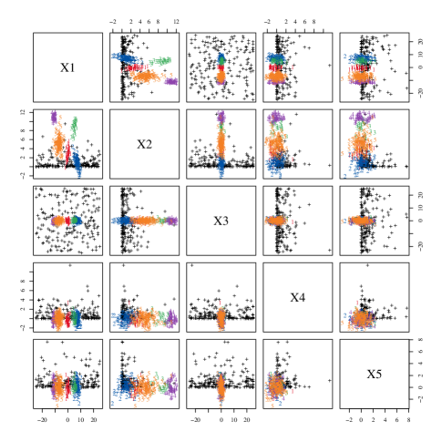
Figure 1: Scatter plots of $n=500$ data points sampled from the AsyNoise design defined in Section 7. Marginals 1 to 5 are represented, further dimensions show a similar pattern. Colors denote the 5 clusters, while noise is represented by the “$+$” symbol.

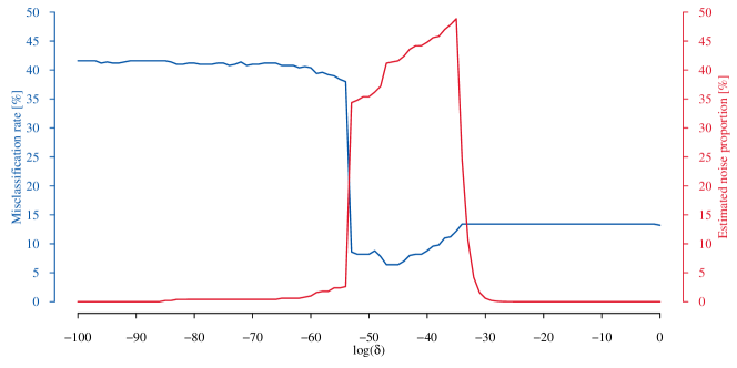
Figure 2: Misclassification rates, and estimated noise proportion by the RIMLE over a grid of $\log(\delta)$ values for the data set in Figure 1.

In AsyNoise (Figure 1) there are 500 observations in 5 moderately separated clusters from student-t distributions with varying degrees of freedom, 187 observations (37.4%) are background noise. Plain Gaussian mixture clustering without noise component fixing the number of clusters $G$ at 5 (as was done for all methods here) using the popular R package mclust of Fraley et al. (2012) puts the clustered points into two big clusters and assigns the noise to the remaining clusters achieving a misclassification rate of 61.4% (i.e., the best misclassification rate that can be achieved by permutation of the cluster labels so that no cluster is identified with the noise). One could wonder whether the data set may be an easy job for clustering methods that take into account outliers, but this is not the case. The mclust software allows for a noise component as defined in Banfield and Raftery (1993), which needs to be initialized. In all situations, mclust chooses an optimal covariance matrix parameterization based on data. The dimensionality of the noise in the given data set seems to be too high for mclust to figure out that all of this really is noise. The resulting misclassification rate is 38%. The TCLUST method implemented in the tclust software of Fritz et al. (2012) with the eigenratio constraint (a tuning parameter, see Section 3.2) set to 100 and the trimming rate set to 33% produces a misclassification rate of 49%. The trimming rate was fixed here imagining that one knows the true underlying expected noise proportion (which is 33% for AsyNoise), which should normally be (unrealistically) advantageous for TCLUST. None of the five underlying clusters is found. tclust also includes the “ctlcurves”-tool for guiding the user toward the choice of a suitable trimming rate. Unfortunately, this graphical tool does not give any clear indication for this data set. The true clusters can be characterized by having a considerably higher density than the noise region, so density based clustering would seem to be another promising approach, but it suffers from the high dimensionality of the data, too. We applied the DBSCAN algorithm (Ester et al. (1996)) using the dbscan R-package of Hahsler (2016). We used various values for its tuning parameters eps (neighborhood radius) and MinPts (minimum number of points in the neighborhood). What happens for reasonable values of MinPts (e.g., 5) is that for small eps everything is classified as noise, and for large eps there are only 2 clusters. In a certain short eps-interval more clusters are found and certain values even deliver 5 clusters. The best partition is found with eps=$4.25$. In this case, DBSCAN’s misclassification rate is 26%; 63% of points are assigned to the noise. The RIMLE method treated in this paper is more appropriate. We computed it for several values of $\log(\delta)$ ($\delta$ is the value of the improper noise density; other constants were chosen as $\gamma=100$ and $\pi_{\max}=0.5$, see Algorithm 2 and Sections 3 for details). Results are shown in Figure 2. When choosing $\log(\delta)$ appropriately, namely $\log(\delta)\in[-53,-36]$, the RIMLE gets the structure of the data set right, and it stably produces a misclassification rate of in the range [6.4%, 11%] with an estimated noise proportion in the range $[34.38\%,45.8\%]$. Values of $\log(\delta)$ below -100 do not change the results. For large values of $\log(\delta)$ too much noise is found, hence the RIMLE’s noise proportion constraint (see Section 3) becomes active and the resulting estimated noise proportion gets close to zero. The OTRIMLE criterion of Coretto and Hennig (2016) selects an optimal value $\log(\delta)=-40$, which is in the region where RIMLE shows its optimal performance. The RIMLE at $\log(\delta)=-40$ produces a misclassification rate of 8.8% with estimated noise proportion equal to 44.8%.

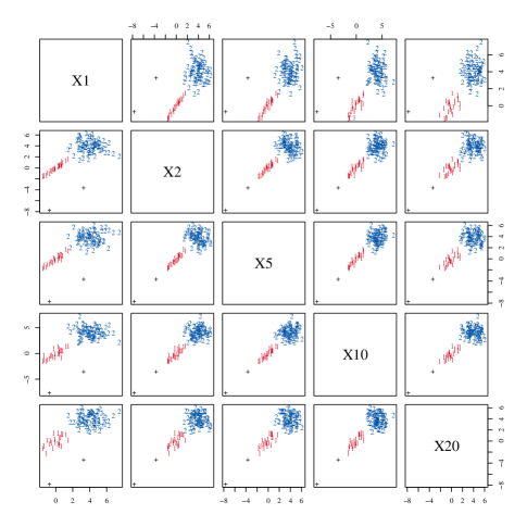
Figure 3: Scatter plots of $n=100$ points sampled from the GEM sampling design defined in Section 7. Marginals 1,2,5,10, and 20 are represented, further dimensions show a similar pattern. Colors denote the 2 clusters, while noise is represented by the “$+$” symbol.

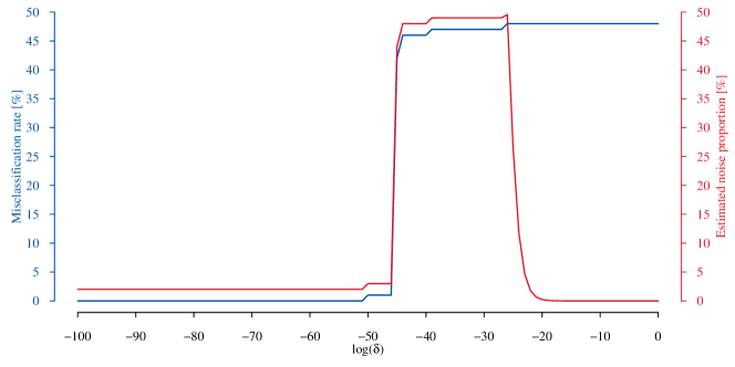
Figure 4: Misclassification rates, and estimated noise proportion by the RIMLE over a grid of $\log(\delta)$ values for the data set in Figure 3.

In GEM (Figure 3), 100 points are sampled from two normal populations with extremely different scatters, 2 points (2%) are outliers almost lying on a hyperplane. These outliers are not extremely separated from the regular points, and this can cause trouble to robust methods. mclust without the noise component assigns the two outliers to cluster 1 and achieves a misclassification rate of 2%, although the estimated mixture parameters are enormously biased. mclust with noise assigns most of the points of the second cluster to the noise component and the resulting misclassification rate is 47%. In this case, the ctlcurves-tool suggests a trimming rate of 6% for TCLUST, but the corresponding misclassification rate is 15%. When the trimming rate is set to 2% (which is the true expected noise proportion for the GEM design), TCLUST misclassifies 11% of the observations. This is because TCLUST gets the covariance structure of the second cluster wrong (see Section 7 for more details). DBSCAN does a better job with this data set, but its performance depends crucially on the appropriate setting of its two tunings. With minPts=3 and eps$\in[6.2,9.6]$, DBSCAN can reconstruct the two clusters and the noise correctly. However, in real situations, the question is how to set these parameters to achieve the best solution. As for the previous data set the RIMLE has been computed for several values of $\log(\delta)$ maintaining all other parameters as before. The result can be seen in Figure 4. For any $-\infty<\log(\delta)\leq-46$ the RIMLE is 100% accurate and estimates a noise proportion of 2%. The OTRIMLE method for the data-driven choice of $\delta$ selects $\log(\delta)=-200$, which is in the region where the RIMLE achieves the best results.

3 Basic definitions

3.1 RIMLE and clustering

The robust improper maximum likelihood estimator (RIMLE) is based on the “noise component”-idea for robustification of the MLE based on the Gaussian mixture model. This models the noise by a uniform distribution, but in fact we are interested in more general patterns of noise or outliers. However, regions of high density are rather associated with clusters than with noise, so the noise regions should be those with the lowest density. This kind of distinction can be achieved by using the uniform density as in Banfield and Raftery (1993), but in the presence of gross outliers the dependence of the uniform distribution on the convex hull of the data causes a robustness problem (Hennig (2004)). The uniform distribution is not really used here as a model for the noise, but rather as a technical device to account for whatever goes on in low density regions. The RIMLE drives this idea further by using an improper uniform distribution the density value of which does not depend on how far awy extreme points in the data are from the main bulk. In the following, assume an observed sample $x_{1},x_{2},\ldots,x_{n},$ where $x_{i}$ is the realization of a random variable $X_{i}\in\mathbb{R}^{p}$ with $p>1$; $X_{1},\ldots,X_{n}$ i.i.d. The goal is to cluster the sample points into $G$ distinct groups. RIMLE then maximizes a pseudo-likelihood, which is based on the improper pseudo-density

$$\psi_{\delta}(x,\theta)=\pi_{0}\delta+\sum_{j=1}^{G}\pi_{j}\phi(x;\mu_{j},\Sigma_{j}),$$ (1)

where $\phi(\cdot,\mu,\Sigma)$ is the Gaussian density with mean $\mu$ and covariance matrix $\Sigma$, $\pi_{0},\pi_{j}\in[0,1]$ for ${j=1,\allowbreak 2,\allowbreak\ldots,\allowbreak G}$, $\pi_{0}+\sum\nolimits_{i=1}^{G}\pi_{j}=1$, while $\delta$ is the improper constant density. The parameter vector $\theta$ contains all Gaussian parameters plus all proportion parameters including $\pi_{0}$, ie. $\theta=(\mu_{1},\ldots,\mu_{G},\operatorname{vect}(\Sigma_{1}),\ldots,\operatorname{vect}(\Sigma_{G}),\pi_{0},\ldots,\pi_{G}),$ where $\operatorname{vect}(A)$ is the vectorized upper (or lower) triangle including the main diagonal of the symmetric square matrix $A$. $\delta$ and the number of Gaussian components $G$ are considered fixed and known. Although this does not define a proper probability model, it yields a useful procedure for data modelled as a proportion of $(1-\pi_{0})$ of a mixture of Gaussian distributions, which have high enough density peaks to be interpreted as clusters plus a proportion $\pi_{0}$ times something unspecified with density $\leq\delta$ (which may even contain further Gaussian components with so few points and/or so large within-component variation that they are not considered as “clusters”).

The definition of the pseudo-model in (1) requires that the value of $\delta$ is fixed in advance. The choice of $\delta$ will be discussed in Section 5.2.

Given the sample improper pseudo-log-likelihood function

$$l_{n}(\theta)=\frac{1}{n}\sum_{i=1}^{n}\log\psi_{\delta}(x_{i},\theta),$$ (2)

the RIMLE is defined as

$$\theta_{n}(\delta)=\mathop{\rm arg\,max}\limits_{\theta\in\Theta_{n}}l_{n}(\theta),$$ (3)

where $\Theta_{n}$ is a constrained parameter space defined in Section 3.2. $\theta_{n}(\delta)$ is then used to cluster points using pseudo posterior probabilities for belonging to the Gaussian components or the improper uniform. These pseudo posterior probabilities are given by

$$\tau_{j}(x_{i},\theta):=\\ \begin{cases}\frac{\pi_{0}\delta}{\psi_{\delta}(x_{i},\theta)}&\text{if}\;j=0\\ \frac{\pi_{j}\phi(x_{i},\mu_{j},\Sigma_{j})}{\psi_{\delta}(x_{i},\theta)}&\text{if}\;{j=1,\allowbreak 2,\allowbreak\ldots,\allowbreak G};\\ \end{cases}\quad\text{for}\;i=1,2,\ldots,n.$$

Points are assigned to the component for which the pseudo posterior probability is maximized. The assignment rule is then given by

$$J(x_{i},\theta):=\mathop{\rm arg\,max}\limits_{j\in\left\{0,1,2,\ldots,G\right\}}\tau_{j}(x_{i},\theta).$$ (4)

The assignment based on maximum posterior probabilities is common to all model-based clustering methods. Here, an improper density is involved, and so these are “pseudo posterior probabilities”.

We also define a population version of the RIMLE for later deriving consistency results for the sequence $\left\{\theta_{n}(\delta)\right\}_{n\in\mathbb{N}}$. Let ${\rm E}_{P}f(x)$ be the expectation of $f(x)$ under $P$. The RIMLE population target function and the constrained parameter set can be obtained by replacing the empirical measure with $P$, and the population version of $l_{n}({\theta})$ is given by

$$L(\theta)={\rm E}_{P}\log(\psi_{\delta}(x,\theta)).$$

Define $L_{G}=\sup_{\theta\in\Theta_{G}(P)}L(\theta)$, where $\Theta_{G}(P)$ is a constrained parameter space defined in Section 3.2.

3.2 The constrained parameter space

Some notation: the $k$th element of $\mu_{j}$ is denoted by $\mu_{j,k}$ for ${k=1,\allowbreak 2,\allowbreak\ldots,\allowbreak p}$ and ${j=1,\allowbreak 2,\allowbreak\ldots,\allowbreak G}$. Let $\lambda_{j,k}$ be the $k$th eigenvalue of $\Sigma_{j}$, define $\Lambda(\theta)=\left\{\lambda_{j,k}:\;{j=1,\allowbreak 2,\allowbreak\ldots,\allowbreak G};\;k=1,2,\ldots,p\right\}$, $\lambda_{\min}(\theta)=\min_{j,k}\{\Lambda(\theta)\}$, $\lambda_{\max}(\theta)=\max_{j,k}\{\Lambda(\theta)\}$.

Remark 1.

The $p$-dimensional Gaussian density can be written in terms of the eigen-decomposition of the covariance matrix:

$$\phi(x;\mu,\Sigma)=(2\pi)^{-\frac{p}{2}}\left(\prod_{k=1}^{p}\lambda_{k}\right)^{-\frac{1}{2}}\exp{\left(-\frac{1}{2}\sum_{k=1}^{p}\lambda_{k}^{-1}(x-\mu)^{\prime}v_{k}v_{k}^{\prime}(x-\mu)\right)},$$

where $\lambda_{k}$ is the $k$-th eigenvalue of $\Sigma$, and $v_{k}$ is its associated eigenvector, for ${k=1,\allowbreak 2,\allowbreak\ldots,\allowbreak p}$. Let $\lambda_{0}=\min\{\lambda_{k};\;{k=1,\allowbreak 2,\allowbreak\ldots,\allowbreak p}\}$. Then, $\lim_{\lambda_{0}\searrow 0}\phi(\mu;\mu,\Sigma)=\infty$, with $\phi(\mu;\mu,\Sigma)=O(\lambda_{0}^{-p/2})$ as $\lambda_{0}\searrow 0$. On the other hand $\lim_{\lambda_{0}\searrow 0}\phi(x;\mu,\Sigma)=0$ for all $x\neq\mu$, with $\phi(x;\mu,\Sigma)=o(\lambda_{0}^{q})$ for any fixed $q$ as $\lambda_{0}\searrow 0$. This implies that

$$\lim_{\lambda_{0}\searrow 0}\;\phi(\mu;\mu,\Sigma)\phi(x;\mu,\Sigma)\to 0\quad\text{for any}\;x\neq\mu$$

Furthermore, each of the density components in $\psi_{\delta}(\cdot)$ can be bounded above in terms of $\lambda_{\max}(\theta)$ and $\lambda_{\min}(\theta)$:

$$\phi(x;\mu_{j},\Sigma_{j})\leq(2\pi\lambda_{\min}(\theta))^{-\frac{p}{2}}\exp\left\{-\frac{1}{2}\lambda_{\max}(\theta)^{-1}\|x-\mu_{j}\|^{2}\right\}\leq(2\pi\lambda_{\min}(\theta))^{-\frac{p}{2}}.$$ (5)

The optimization problem in (3) requires that $\Theta_{n}$ is suitably defined, otherwise $\theta_{n}(\delta)$ may not exist. Consider a sequence $(\theta_{m})_{m\in\mathbb{N}}$, as discovered by Kiefer and Wolfowitz (1956), the likelihood of a Gaussian mixtures degenerates if $\lambda_{1,1,m}\searrow 0$ if $\mu_{1,m}=x_{1}$, and this holds for (2), too. We here use the eigenratio constraint

$$\lambda_{\max}(\theta)/\lambda_{\min}(\theta)\leq\gamma<+\infty$$ (6)

with a constant $\gamma\geq 1$, where $\gamma=1$ constrains all component covariance matrices to be spherical and equal, as in $k$-means clustering. This type of constraint has been proposed by Dennis (1981), while Hathaway (1985) showed consistency of the scale-ratio constrained MLE for one-dimensional Gaussian mixtures. Ingrassia (2004) and Ingrassia and Rocci (2007) introduced EM algorithms for implementing these constraints for multivariate datasets. TCLUST by García-Escudero et al. (2008) and García-Escudero et al. (2014) also makes use of eigenratio constraints. Moreover there are a number of alternative constraints, see Ingrassia and Rocci (2011); Gallegos and Ritter (2009). It may be seen as a disadvantage of (6) that the resulting estimator will not be affine equivariant (this would require allowing $\lambda_{\max}(\theta)/\lambda_{\min}(\theta)\to\infty$ within any component). Affine equivariance can be achieved by defining a sphered version of the RIMLE as

$$\theta_{n}^{*}(\delta)=\theta_{n}^{*}(\delta,x_{1},\ldots,x_{n})=\theta_{n}(\delta,x_{1}^{*},x_{2}^{*},\ldots,x_{n}^{*})$$

with $x_{i}^{*}=A(x_{i}-m),\ i=1,\dots,n$, where $S(x_{1},\ldots,x_{n})^{-1}=A^{\prime}A$; $S(x_{1},\ldots,x_{n})$ could be the sample covariance matrix or another scale matrix and $m$ the mean vector or another location estimator. This yields affine equivariance because the sphered versions of $\{x_{1},\ldots,x_{n}\}$ and $\{Bx_{1}+b,\ldots,Bx_{n}+b\}$ with some invertible $p\times p$-matrix $B$ and $b\in\mathbb{R}^{p}$ are the same. Affine equivariance is not necessarily desirable though, see Hennig (2015a), Sec. 31.3.4.

This defines the parameter space

$$\tilde{\Theta}:=\left\{\theta:\;\;\pi_{j}\geq 0\;\forall j\geq 1,\;\pi_{0}+\sum_{j=1}^{G}\pi_{j}=1;\;\frac{\lambda_{\max}(\theta)}{\lambda_{\min}(\theta)}\leq\gamma\right\}.$$ (7)

Occasionally, later, the notation $\|\theta\|$ will refer to the Euclidean norm of a vector pieced together from all the parameters collected in $\theta$, in which all covariance matrices are interpreted as subvectors of all the matrix entries.

Although (6) ensures the boundedness of the likelihood in standard mixture models and TCLUST, for RIMLE this is not enough. The Gaussian components could degenerate on a few points and all other points could be fitted by the improper uniform component. Therefore we impose an additional constraint:

$$\frac{1}{n}\sum_{i=1}^{n}\tau_{0}(x_{i},\theta)\leq\pi_{\text{max}},$$ (8)

for fixed $0<\pi_{\max}<1$. The quantity $n^{-1}\sum_{i=1}^{n}\tau_{0}(x_{i},\theta)$ can be interpreted as the estimated proportion of noise points. This constraint depends on the dataset. Unfortunately the similar looking constraint $\pi_{0}\leq\pi_{\max}$ independent of the data will not do, because this could not stop more than a portion of $\pi_{0}$ points to be fitted by the improper uniform component.

There is therefore a constrained effective parameter space for RIMLE estimation depending on the dataset:

$$\Theta_{n}:=\left\{\theta\in\tilde{\Theta}:\;\;\pi_{j}\geq 0\;\forall j\geq 1,\;\pi_{0}+\sum_{j=1}^{G}\pi_{j}=1;\;\frac{1}{n}\sum_{i=1}^{n}\tau_{0}(x_{i},\theta)\leq\pi_{\text{max}};\;\frac{\lambda_{\max}(\theta)}{\lambda_{\min}(\theta)}\leq\gamma\right\}.$$ (9)

Analogously, existence and consistency of the RIMLE functional can only be showed on a parameter subset of $\tilde{\Theta}$ that depends on the underlying distribution and enforces that enough probability mass is fitted by Gaussian components rather than the improper uniform:

$$\Theta_{G}(P):=\left\{\theta\in\tilde{\Theta}:\;\pi_{j}\geq 0\;\forall j\geq 1;\;\pi_{0}+\sum_{j=1}^{G}\pi_{j}=1;\;{\rm E}_{P}\frac{\pi_{0}\delta}{\psi_{\delta}(x,\theta)}\leq\pi_{\max};\;\frac{\lambda_{\max}(\theta)}{\lambda_{\min}(\theta)}\leq\gamma\right\}.$$ (10)

4 RIMLE existence and consistency

We first show existence of the RIMLE for finite samples Let $\#(A)$ denote the cardinality of the set $A$. Let $\underline{x_{n}}=\{x_{1},x_{2},\ldots,x_{n}\}$. Lemma 1 concerns the important case of plain Gaussian mixtures ($\delta=0$) and requires a weaker assumption A0(a) for existence than A0 required for the RIMLE with $\delta>0$. Here are some assumptions:

A0(a)

$\#(\underline{x_{n}})>G$.

A0   

$\#(\underline{x_{n}})>G+\lceil n\pi_{\max}\rceil$.

Lemma 1.

Assume A0(a), $\delta=0$. Let $(\theta_{m})_{m\in\mathbb{N}}$ be a sequence such that $\lambda_{\max}(\theta_{m})/\lambda_{\min}(\theta_{m})$ $\leq\gamma$. Assume also that for some ${j=1,\allowbreak 2,\allowbreak\ldots,\allowbreak G}$ and ${k=1,\allowbreak 2,\allowbreak\ldots,\allowbreak p}$, $\lambda_{k,j,m}\searrow 0$ as $m\to\infty$; then $\sup l_{n}(\theta_{m})\to-\infty.$

Proof.

$\lambda_{k,j,m}\searrow 0$ implies $\lambda_{\max}(\theta_{m})\searrow 0,\ \lambda_{\min}(\theta_{m})\searrow 0$ at the same speed because of (6). Assume w.l.o.g. (otherwise consider a suitable subsequence) that $(\theta_{m})_{m\in\mathbb{N}}$ is such that $\mu_{j,m},$ ${j=1,\allowbreak 2,\allowbreak\ldots,\allowbreak G}$ either leave every compact set for $m$ large enough or converge, and assume w.l.o.g., that if their limits are in $\{x_{1},\ldots,x_{n}\}$, they are in $\underline{x_{G}}=\{x_{1},\ldots,x_{G}\}$. A0(a) implies that $\exists\ x_{i}\not\in\underline{x_{G}}$, and $\exists\nu>0$ such that for all such $x_{i},\ {j=1,\allowbreak 2,\allowbreak\ldots,\allowbreak G}$ and large enough $m:\|x_{i}-\mu_{j,m}\|\geq\nu$. Because the likelihood

$$\mathcal{L}_{n}(\theta_{m})=\prod_{x_{i}\in\underline{x_{G}}}\Bigl{\{}\sum_{j=1}^{G}\pi_{j}\phi(x_{i};\mu_{j,m},\Sigma_{j,m})\Bigr{\}}\prod_{x_{i}\not\in\underline{x_{G}}}\Bigl{\{}\sum_{j=1}^{G}\pi_{j}\phi(x_{i};\mu_{j,m},\Sigma_{j,m})\Bigr{\}},$$ (11)

and Remark 1, the first product is of order $O(\lambda_{\min}(\theta_{m})^{-p/2})^{G}$, and the second one of order $o(\lambda_{\min}(\theta_{m})^{q})$ for any fixed $q$, which implies that $\mathcal{L}_{n}(\theta_{m})\to 0$ and $l_{n}(\theta_{m})\to-\infty$. ∎

Lemma 2.

Assume A0, $\delta>0$. $(\theta_{m})_{m\in N}$ is a sequence in $\Theta_{n}$. Assume also that for some ${j=1,\allowbreak 2,\allowbreak\ldots,\allowbreak G}$ and ${k=1,\allowbreak 2,\allowbreak\ldots,\allowbreak p}$, $\lambda_{k,j,m}\searrow 0$ as $m\to\infty$. Then $l_{n}(\theta_{m})\to-\infty.$

Proof.

Using the definitions of the proof of Lemma 1, instead of (11) now

$$\mathcal{L}_{n}(\theta_{m})=\prod_{x_{i}\in\underline{x_{G}}}\Bigl{\{}\pi_{0,m}\delta+\sum_{j=1}^{G}\pi_{j}\phi(x_{i};\mu_{j,m},\Sigma_{j,m})\Bigr{\}}\prod_{x_{i}\not\in\underline{x_{G}}}\Bigl{\{}\pi_{0,m}\delta+\sum_{j=1}^{G}\pi_{j}\phi(x_{i};\mu_{j,m},\Sigma_{j,m})\Bigr{\}}$$ (12)

has to be considered, so that the limit behaviour of $(\pi_{0,m})_{m\in\mathbb{N}}$ is relevant. (8) implies

$$\frac{1}{n}\sum_{x_{i}\in\underline{x_{G}}}\left(1+\sum_{j=1}^{G}\frac{\pi_{j}\phi(x_{i},\mu_{j,m},\Sigma_{j,m})}{\pi_{0,m}\delta}\right)^{-1}+\frac{1}{n}\sum_{x_{i}\not\in\underline{x_{G}}}\left(1+\sum_{j=1}^{G}\frac{\pi_{j}\phi(x_{i},\mu_{j,m},\Sigma_{j,m})}{\pi_{0,m}\delta}\right)^{-1}\leq\pi_{\max}.$$ (13)

Suppose that $(\pi_{0,m})_{m\in\mathbb{N}}$ does not converge to zero as $O(\phi(x_{i},\mu_{j,m},\Sigma_{j,m}))$ for at least one $x_{i}\not\in\underline{x_{G}}$. For $m\to\infty$, the left term of (13) is $\geq 0$, and the right term (at least a subsequence) converges to $\frac{\#(\underline{x_{n}}\setminus\underline{x_{G}})}{n}$, which A0 requires to be $>\pi_{\max}$ with contradiction, thus $\pi_{0,m}=O(\phi(x_{i},x_{j},\Sigma_{j,m}))$. Therefore, by the same argument as in the proof of Lemma 1, the right product in (12) vanishes fast enough so that $l_{n}(\theta_{m})\to-\infty$. ∎

From these Lemmas:

Theorem 1 (Finite Sample Existence).

Assume A0. Then $\theta_{n}(\delta)$ exists for all $\delta\geq 0$.

Proof.

$\Theta_{n}$ depends on $\delta$ via (8). $\Theta_{n}$ is not empty for any $\delta$, because for any fixed values of the other parameters, small enough $\pi_{0}$ will fulfil (8). Next show that there exists a compact set $K_{n}\subset\Theta_{n}$ such that $\sup_{\theta\in K_{n}}l_{n}(\theta)=\sup_{\theta\in\Theta_{n}}l_{n}(\theta)$.
Step A: consider $\theta$ such that $\pi_{1}=1$, $\mu_{1}=x_{1}$, $\Sigma_{j}=I_{p}$ for all ${j=1,\allowbreak 2,\allowbreak\ldots,\allowbreak G}$, arbitrary $\mu_{j}$ and $\pi_{j}=0$ for all $j\neq 1$. For this, $l_{n}(\theta)=\sum_{i=1}^{n}\log\phi(x_{i};x_{1},\Sigma_{1})>-\infty$, thus $\sup_{\theta\in\Theta_{n}}l_{n}(\theta)>-\infty$.
Step B: consider a sequence $(\dot{\theta}_{m})_{m\in N}$. It needs to be proved that if $(\dot{\theta}_{m})_{m\in N}$ leaves a suitably chosen compact set $K_{n}$, it cannot achieve as large values of $l_{n}$ as one could find within $K_{n}$. Lemma 2 (Lemma 1 for $\delta=0$) rules out the possibility of any $\lambda_{k,j,m}\searrow 0$.
Step C: (5) implies that $l_{n}(\theta)$ can be bounded from above in terms of $\pi_{0},\lambda_{\min}$ and $\delta$:

$$l_{n}(\theta)=\frac{1}{n}\sum_{i=1}^{n}\log\left(\pi_{0}\delta+\sum_{j=1}^{G}\pi_{j}\phi(x_{i};\mu_{j},\Sigma_{j})\right)\leq\log\left(\pi_{0}\delta+(1-\pi_{0})(2\pi\lambda_{\min}(\theta))^{-\frac{p}{2}}\right).$$

Consider $\dot{\theta}\in\Theta_{n}$ such that $\dot{\lambda}_{k,j}<+\infty$ for all ${k=1,\allowbreak 2,\allowbreak\ldots,\allowbreak p}$ and ${j=1,\allowbreak 2,\allowbreak\ldots,\allowbreak G}$ (using the obvious notation of components of “dotted” parameter vectors). Also consider a sequence $(\ddot{\theta}_{m})_{m\in\mathbb{N}}$ such that $\ddot{\theta}_{m}\to\ddot{\theta}$ where $\ddot{\theta}$ is equal to $\dot{\theta}$ except that $\ddot{\lambda}_{k,j,m}\to+\infty$ for some $k\in\{1,\ldots,p\}$ and $j\in\{1,\ldots,G\}$. By (6), $\lambda_{\min}(\ddot{\theta}_{m})\to+\infty$ and thus $l_{n}(\ddot{\theta}_{m})\to\log(\ddot{\pi}_{0}\delta)$. Clearly $\ddot{\pi}_{0}<1$ because otherwise $n^{-1}\sum_{i=1}^{n}\tau_{0}(x_{i},\ddot{\theta})=1$, violating (8). Therefore $\lim_{m\to\infty}l_{n}(\ddot{\theta}_{m})\leq l_{n}(\dot{\theta})$.
Step D: now consider $||\dot{\mu}_{j,m}||\to+\infty$, for $j=1$, w.l.o.g. Choose $\ddot{\theta}_{m}$ equal to $\dot{\theta}_{m}$ except now $\ddot{\mu}_{1,m}=0$ for all $m$. Note that $\phi(x_{i};\dot{\mu}_{1,m},\dot{\Sigma}_{1})\to 0$ for all ${i=1,\allowbreak 2,\allowbreak\ldots,\allowbreak n}$, which implies that $\psi_{\delta}(x_{i},\dot{\theta}_{m})<\psi_{\delta}(x_{i},\ddot{\theta}_{m})$ for large enough $m$, for which then $l_{n}(\dot{\theta}_{m})<l_{n}(\ddot{\theta}_{m})$. Applying this argument to all $j$ with $||\dot{\mu}_{j,m}||\to+\infty$ shows that better $l_{n}$ can be achieved inside a compact set.

Continuity of $l_{n}$ now guarantees existence of $\theta_{n}(\delta)$. ∎

We now derive consistency for the sequence $\left\{\theta_{n}(\delta)\right\}_{n\in\mathbb{N}}$ as estimator of $L_{G}$. Consistency of the RIMLE can be achieved only if $L_{G}$ exists. In order to ease the notation we define $\eta(x,\theta)=\sum_{j=1}^{G}\pi_{j}\phi(x;\mu_{j},\Sigma_{j}).$ Consider the following assumptions on $P$:

A1

For every $x_{1},\ldots,x_{G}\in\mathbb{R}^{p}:P\{x_{1},\ldots,x_{G}\}<1-\pi_{max}$.

A2

$L_{G}>L_{G-1}$, where for $G\in\mathbb{N}$ let $L_{G}=\sup_{\theta\in\Theta_{G}(P)}L(\theta)$.

A3

There exist $\epsilon_{1},\epsilon_{2}>0$ so that for every $\theta$ with $\pi_{0}<\epsilon_{1}:$ $L(\theta)\leq L_{G}-\epsilon_{2}$.

Remark 2.

Assumption A1 requires that no set of $G$ points carries probability $1-\pi_{\max}$ or more. Otherwise the log-likelihood can be driven to $\infty$ by fitting $G$ mixture components to $G$ points with all covariance matrix eigenvalues converging to zero. The improper noise component could take care of all other points. Note that assumptions A2 and A3 are not both required, but only any single one of them.

A2 states that $G$ mixture components fit the data better than $G-1$. If this is not the case, there is at least one redundant component, and one cannot make sure that $L(\theta)$ is bounded away from $L_{G}$ for large $n$ in some distance from the “true” RIMLE-functional as the redundant component can be moved around, see Theorem 2. In case that A2 is not fulfilled, a weaker result can still be achieved, namely the existence of a not necessarily unique consistent sequence of local maximizers of $l_{n}$. This requires A3, which states that a noise proportion bounded away from zero is required for maximizing $L$. If neither A2 nor A3 are fulfilled, $P$ can be fitted perfectly by fewer than $G$ mixture components and no noise. In this case one cannot stop the remaining mixture components from leaving every compact set, and therefore one cannot expect consistency of all components for any method; as long as there is still noise bounded away from zero, those mixture components still can contribute to fitting what otherwise would be noise, and fits become worse if these degenerate.

Note that this is less often the case than one might expect; for example, a plain Gaussian mixture with $G-1$ components may still fulfill A3: if the density of one of the components is uniformly smaller than $\delta$, a better pseudo-likelihood can obviously be achieved by assigning its proportion to the noise component than by choosing $\pi_{0}=\pi_{G}=0$ and otherwise the true parameters. A Gaussian component that “looks like noise” rather than like a “cluster” will be treated as noise.

Lemma 3.

For any probability measure $P$ on $\mathbb{R}^{p}$, $L_{G}>-\infty$.

Proof.

Choose compact $K\subset\mathbb{R}^{p}$ with $P(K)>0$. Let $q=1-P(K)$ and choose $K$ big enough that $\pi_{\max}>q$. Choose $\mu_{1}={\rm E}_{P}(x|x\in K),\ \Sigma_{1}={\rm Cov}_{P}(x|x\in K),\ \pi_{2}=\ldots=\pi_{G}=0$. If all eigenvalues of $\Sigma_{1}$ are zero, choose $\Sigma_{1}=I_{p}$. Let $\lambda_{\max,1}$ be the largest eigenvalue of $\Sigma_{1}$. If $\lambda_{\max,1}/\lambda_{i,1}>\gamma$ for any eigenvalue $\lambda_{i,1}$ of $\Sigma_{1}$, modify $\Sigma_{1}$ by replacing all eigenvalues smaller than $\gamma\lambda_{\max,1}$ by $\gamma\lambda_{\max,1}$ in its spectral decomposition. Let $\phi_{\min}=\min_{x\in K}\phi(x,\mu_{1},\Sigma_{1})>0$. Choose

$$\pi_{0}=\frac{(\pi_{\max}-q)\phi_{\min}}{2((1-\pi_{\max})\delta+(\pi_{\max}-q)\phi_{\min})}>0,\ \pi_{1}=1-\pi_{0}.$$

Observe that the resulting $\theta\in\Theta_{G}(P)$ (with all other parameters chosen arbitrarily) by

$${\rm E}_{P}\frac{\pi_{0}\delta}{\psi_{\delta}(x,\theta)} =\int_{K}\frac{\pi_{0}\delta}{\pi_{0}\delta+\eta(x,\theta)}dP(x)+\int_{K^{c}}\frac{\pi_{0}\delta}{\pi_{0}\delta+\eta(x,\theta)}dP(x)\leq$$

$$\leq(1-q)\frac{\pi_{0}\delta}{\pi_{0}\delta+(1-\pi_{0})\phi_{\min}}+q.$$

This is smaller than $\pi_{\max}$ if $\pi_{0}<\frac{(\pi_{\max}-q)\phi_{\min}}{(1-\pi_{\max})c+(\pi_{\max}-q)\phi_{\min}}$. Furthermore, $L(\theta)\geq(1-q)\log(\pi_{0}\delta+(1-\pi_{0})\phi_{\min})+q\log(\pi_{0}\delta)>-\infty$. ∎

Lemma 4.

Assume A1. There are $\lambda^{*}_{\min}>0,\ \lambda^{*}_{\max}<\infty,\ \epsilon>0$, so that

(a)

$L(\theta)\leq L_{G}-\epsilon$ for every $\theta$ with $\lambda_{\min}(\theta)<\lambda_{\min}^{*}$ or $\lambda_{\max}(\theta)>\lambda_{\max}^{*}$,

(b)

for $x_{1},x_{2},\ldots$ i.i.d. with ${\cal L}(x_{1})=P$, for sequences $(\theta_{n})_{n\in\mathbb{N}}$ with $\lambda_{\min}(\theta_{n})<\lambda_{\min}^{*}$ or $\lambda_{\max}(\theta_{n})>\lambda_{\max}^{*}$ for large enough $n$: $l_{n}(\theta_{n})\leq l_{n}(\theta_{n}(\delta))-\epsilon$ a.s.

Proof.

Start with part (a). First consider a sequence $\left\{\theta_{m}\right\}_{m\in\mathbb{N}}\in\Theta_{G}(P)^{\mathbb{N}}$ with $\lambda_{\max}(\theta_{m})\to\infty$. The eigenvalue ratio constraint forces all covariance matrix eigenvalues to infinity, and therefore $\sup_{x}\phi(x,\mu_{j,m},\Sigma_{j,m})\searrow 0$. But this means that ${\rm E}_{P}\frac{\pi_{0}\delta}{\psi_{\delta}(x,\theta)}\to 1>\pi_{\max}$ and $\theta_{m}\not\in\Theta_{G}(P)$ eventually, unless $\pi_{0,m}\searrow 0$, too. If the latter is the case, $\psi_{\delta}(x,\theta)\searrow 0$ uniformly over all $x$ and $L(\theta_{m})\searrow-\infty$, which together with Lemma 3 makes it impossible that $L(\theta_{m})$ is close to $L_{G}$ for $m$ large enough and $\lambda_{\max}(\theta_{m})$ too large, proving the existence of the upper bound $\lambda^{*}_{\max}<\infty$ as required.
Now consider a sequence $\left\{\theta_{m}\right\}_{m\in\mathbb{N}}\in\Theta_{G}(P)^{\mathbb{N}}$ with $\lambda_{\min}(\theta_{m})\to 0$. Define

$$A_{m,\epsilon}=\left\{x:\;\min_{{j=1,\allowbreak 2,\allowbreak\ldots,\allowbreak G}}\|x-\mu_{j,m}\|>\epsilon\right\}.$$

A1 ensures that for $0<\epsilon_{3}$ there exists $\epsilon>0$ so that for all $m\in\mathbb{N}:$ $P(A_{m,\epsilon})\geq\pi_{\max}+\epsilon_{3}$. Based on (5) derive an upper bound for $\pi_{0,m}$ from the constraint $\int\frac{\pi_{0,m}\delta}{\pi_{0,m}\delta+\eta(x,\theta_{m})}dP(x)\leq\pi_{\max}$:

$$\int\frac{\pi_{0,m}\delta}{\pi_{0,m}\delta+\eta(x,\theta_{m})}dP(x) =\int_{A_{m,\epsilon}}\frac{\pi_{0,m}\delta}{\pi_{0,m}\delta+\eta(x,\theta_{m})}dP(x)+\int_{A_{m,\epsilon}^{c}}\frac{\pi_{0,m}\delta}{\pi_{0,m}\delta+\eta(x,\theta_{m})}dP(x)\geq$$

$$\geq P(A_{m,\epsilon})\frac{\pi_{0,m}\delta}{\pi_{0,m}\delta+\max_{x\in A_{m,\epsilon}}\eta(x,\theta_{m})},$$

which by (5) implies

$$\pi_{0,m}\leq\frac{\pi_{\max}\max_{x\in A_{m,\epsilon}}\eta(x,\theta_{m})}{\delta(P(A_{m,\epsilon})-\pi_{\max})}\leq\frac{\pi_{\max}\exp(-\frac{\epsilon^{2}}{2\gamma\lambda_{\min}(\theta_{m})})}{\delta\epsilon_{3}(2\pi)^{p/2}\lambda_{\min}(\theta_{m})^{p/2}}.$$

For the log-likelihood,

$$L(\theta_{m}) =\int_{A_{m,\epsilon}}\log(\pi_{0,m}\delta+\eta(x,\theta_{m}))dP(x)+\int_{A_{m,\epsilon}^{c}}\log(\pi_{0,m}\delta+\eta(x,\theta_{m}))dP(x)\leq$$

$$\leq\int_{A_{m,\epsilon}}\log\left(\frac{\delta\pi_{\max}\exp(-\frac{\epsilon^{2}}{2\gamma\lambda_{\min}(\theta_{m})})}{\delta\epsilon_{3}(2\pi)^{p/2}\lambda_{\min}(\theta_{m})^{p/2}}+\frac{\exp(-\frac{\epsilon^{2}}{2\gamma\lambda_{\min}(\theta_{m})})}{(2\pi)^{p/2}\lambda_{\min}(\theta_{m})^{p/2}}\right)dP(x)+$$

$${}{\leavevmode\nobreak\ \leavevmode\nobreak\ \leavevmode\nobreak\ }+\int_{A_{m,\epsilon}^{c}}\log\left(\frac{\delta\pi_{\max}\exp(-\frac{\epsilon^{2}}{2\gamma\lambda_{\min}(\theta_{m})})}{\delta\epsilon_{3}(2\pi)^{p/2}\lambda_{\min}(\theta_{m})^{p/2}}+\frac{1}{(2\pi)^{p/2}\lambda_{\min}(\theta_{m})^{p/2}}\right)dP(x)\leq$$

$$\leq P(A_{m,\epsilon})\left(-\frac{c_{1}}{\lambda_{\min}(\theta_{m})}-c_{2}\log(\lambda_{\min}(\theta_{m}))+c_{3}\right)+$$

$${}{\leavevmode\nobreak\ \leavevmode\nobreak\ \leavevmode\nobreak\ }+P(A_{m,\epsilon}^{c})\left(o(1)-c_{4}\log(\lambda_{\min}(\theta_{m}))+c_{5}\right)=$$

$$=-\frac{c_{6}}{\lambda_{\min}(\theta_{m})}-c_{7}\log(\lambda_{\min}(\theta_{m}))+c_{8}$$

for positive constants $c_{1},c_{2},c_{4},c_{6},c_{7}$ and constants $c_{3},c_{5},c_{8}$, all independent of $\theta_{m}$. If $\lambda_{\min}(\theta_{m})\searrow 0$, this implies $L(\theta_{m})\searrow-\infty$, proving together with Lemma 3 the existence of the lower bound $\lambda^{*}_{\min}>0$.

Part (b) holds because if $(\theta_{m})_{m\in\mathbb{N}}$ is chosen as above for $m=n\to\infty$ and $P$ is replaced by the empirical distribution $P_{n}$, Glivenko-Cantelli enforces $P_{n}(A_{n,\epsilon})-P(A_{n,\epsilon})\to 0$ a.s. Glivenko-Cantelli applies because the class of all $A_{m,\epsilon}$ is a subset of the class of intersections of the complements of all closed balls, and therefore a Vapnik-Chervonenkis class, see van der Vaart and Wellner (1996). The argument carries over using all other integrals in the finite sample-form, i.e., w.r.t. $P_{n}$. Lemma 3 carries over because $l_{n}(\theta)\to L(\theta)$ a.s. by the strong law of large numbers for $\theta$ with $L(\theta)>-\infty$. ∎

Remark 3.

Lemma 4 (a) and (5) imply that for all $\theta$ with $L(\theta)>L_{G}-\epsilon$, ${j=1,\allowbreak 2,\allowbreak\ldots,\allowbreak G}$ and all $x$:

$$\phi(x,\mu_{j},\Sigma_{j})\leq\phi_{\max}=\frac{1}{(2\pi)^{p/2}(\lambda_{\min}^{*})^{p/2}}.$$

This implies $L_{G}<\infty$.

The same holds because of Lemma 4 (b) for $x_{1},x_{2},\ldots$ i.i.d. with ${\cal L}(x_{1})=P$ for large enough $n$ a.s. for all $\theta$ with $l_{n}(\theta)>l_{n}(\theta_{n}(\delta))-\epsilon$.

Lemma 5.

Assume A1 and A2. There is a compact set $K\subset\mathbb{R}^{p}$ so that

(a)

$L$ reaches its supremum for $\mu_{1},\ldots,\mu_{G}\in K$ and is bounded away from the supremum if not all of $\mu_{1},\ldots,\mu_{G}\in K$ (i.e., $\exists\epsilon_{4}>0$ so that it is $\leq\sup L-\epsilon_{4}$) ,

(b)

for $x_{1},x_{2},\ldots$ i.i.d. with ${\cal L}(x_{1})=P$ for large enough $n$, $l_{n}$ reaches its supremum for $\mu_{1},\ldots,\mu_{G}\in K$ and is bounded away from the supremum if not all of $\mu_{1},\ldots,\mu_{G}\in K$, a.s.

Proof.

Start with part (a). Consider a sequence $\left\{\theta_{m}\right\}_{m\in\mathbb{N}}\in\Theta_{G}(P)^{\mathbb{N}}$ with $\|\mu_{jm}\|\to\infty$ for $j=1,\ldots,k,\ 1\leq k<G$ and a compact set $K$ with $\mu_{jm}\in K$ for $j>k$. Let

$$A_{m}=\left\{x:\ \forall j\in\left\{1,\ldots,k\right\}:\phi(x,\mu_{j,m},\Sigma_{j,m})\leq\epsilon_{m}\sum_{l=k+1}^{G}\pi_{l,m}\phi(x,\mu_{l,m},\Sigma_{l,m})\right\},$$

where $\epsilon_{m}\searrow 0$ slowly enough that $P(A_{m})\to 1$. Let $\pi^{*}_{m}=\sum_{j=1}^{k}\pi_{j,m}$. Let $\theta_{(G-k),m}$ for $m\in\mathbb{N}$ be defined by $\pi_{0,(G-k),m}=\pi_{0,m},\ \pi_{(j-k),(G-k),m}=\pi_{j,m}(1-\pi_{0,m})(1-\pi^{*}_{m}-\pi_{0,m})^{-1}$ for $j=k+1,\ldots,G$ accompanied by the $\mu_{j},\Sigma_{j}$-parameters belonging to the components $k+1,\ldots,G$ of $\theta_{m}$. Observe, using Remark 3,

$$L(\theta_{m}) =\int_{A_{m}}\log(\psi_{\delta}(x,\theta_{m}))dP(x)+\int_{A_{m}^{c}}\log(\psi_{\delta}(x,\theta_{m}))dP(x)\leq$$

$$\leq\int_{A_{m}}\log((1+\epsilon_{m})\psi_{\delta}(x,\theta_{(G-k)m}))dP(x)+P(A_{m}^{c})\log(\delta+\phi_{max})$$

implying $L(\theta_{(G-k)m})-L(\theta_{m})\to 0$. ${\rm E}_{P}[\pi_{0,(G-k),m}\delta(\psi_{\delta}(x,\theta_{(G-k)m}))^{-1}]\leq\pi_{\max}$ will be fulfilled for $m$ large enough because it is fulfilled for $\theta_{m}$ by definition and $\psi_{\delta}(x,\theta_{(G-k),m})>\psi_{\delta}(x,\theta_{m})$ on $A_{m}$ with $P(A_{m})\to 1$. $L(\theta_{(G-k)m})<L_{G-1}$ implies that, because of A2, $\theta_{m}$ is bounded away from $L_{G}$.

Regarding existence of a maximum with $\mu_{1},\ldots,\mu_{G}\in K$, observe that with Remark 3, $\psi_{\delta}(x,\theta)$ can be bounded by $\delta+\phi_{max}$ for all $\theta$ for which $L(\theta)>L_{G}-\epsilon$. Now consider a sequence $(\theta_{m})_{m\in\mathbb{N}}$ so that $\forall m:\ \mu_{1m},\ldots,\mu_{Gm}\in K$, with the notation of Lemma 4, $\lambda^{*}_{min}\leq\lambda_{min}(\theta_{m})\leq\lambda_{max}(\theta_{m})\leq\lambda^{*}_{max}$ and $L(\theta_{m})\to L_{G}$. Because of compactness, w.l.o.g., $\theta_{m}\to\theta_{+}$ and, using Fatou’s Lemma, $L_{G}=\lim_{m\to\infty}L(\theta_{m})\leq E_{P}\limsup_{m}\psi_{\delta}(x,\theta_{m})=L(\theta_{+})\leq L_{G}$.

Part (b) holds because if $(\theta_{m})_{m\in\mathbb{N}}$ is chosen as above for $m=n\to\infty$ and $P$ is replaced by the empirical distribution $P_{n}$, Glivenko-Cantelli enforces $P_{n}(A_{n})-P(A_{n})\to 0$ a.s. Glivenko-Cantelli applies here because a sequence of closed balls $(B_{n})_{n\in\mathbb{N}}$ can be constructed so that $B_{n}\subseteq A_{n},\ P(B_{n})\to 1$ a.s.; the closed balls are a Vapnik-Chervonenkis class, and $P_{n}(A_{n})\geq P_{n}(B_{n})\to 1$ a.s. Furthermore, for $\theta\in\Theta_{G}(P)$ with $L(\theta)>L_{G-1}$: $l_{n}(\theta)\to L(\theta)$ a.s. by the strong law of large numbers, so that for large enough $n$: $\sup_{\theta\in\Theta_{G}(P)}l_{n}(\theta)>L_{G-1}$ a.s. On the other hand, $\theta_{(G-k),n}$ can be chosen optimally in a compact set $K$ because of Lemma 4, within which $l_{n}$ converges uniformly to $L$ a.s. (Theorem 2 in Jennrich (1969)), and therefore, $\limsup_{n\to\infty}l_{n}(\theta_{(G-k),n})\leq L_{G-1}$. With these ingredients, the argument of part (a) carries over. ∎

Lemma 6.

Assume A1 and A3. There is a compact set $K\subset\mathbb{R}^{p}$ so that

(a)

$L$ reaches its supremum for $\mu_{1},\ldots,\mu_{G}\in K$,

(b)

for $x_{1},x_{2},\ldots$ i.i.d. with ${\cal L}(x_{1})=P$, there exists a sequence $(\tilde{\theta}_{n})_{n\in\mathbb{N}}$ maximizing $l_{n}$ locally for $\mu_{1},\ldots,\mu_{G}\in K$ so that $l_{n}(\tilde{\theta}_{n})\to L_{G}$ a.s., and a.s. there is no sequence $\theta_{n}\in\Theta_{G}(P)$ so that $\limsup_{n\to\infty}l_{n}(\theta_{n})>L_{G}$.

Proof.

Start with part (a). Consider a sequence $\left\{\theta_{m}\right\}_{m\in\mathbb{N}}\in\Theta_{G}(P)^{\mathbb{N}}$ with $\|\mu_{j,m}\|\to\infty$ for $j=1,\ldots,k,\ 1\leq k<G$ (the case $k=G$ is treated at the end), and a compact set $K$ with $\mu_{j,m}\in K$ for $j>k$. By selecting a subsequence if necessary, assume that there exists $\mu_{j}=\lim_{m\to\infty}\mu_{j,m},$ $\Sigma_{j}=\lim_{m\to\infty}\Sigma_{j,m}$ for $k+1\leq j\leq G$ and that $\pi_{j,m}$ converge for $j=0,\ldots,G$. Let $j^{*}=\mathop{\rm arg\,max}\limits_{k+1\leq j\leq G}{\rm E}_{P}\phi(x,\mu_{j},\Sigma_{j})$. Suppose $L(\theta_{m})\nearrow L_{G}$ monotonically and, by A3, assume $\pi_{0,m}>\epsilon_{1}$.

Consider first the case $\sum_{j=1}^{k}\pi_{j,m}\to\epsilon_{3}>0$. Construct another sequence $\left\{\theta_{*m}\right\}_{m\in\mathbb{N}}\in\Theta_{G}(P)^{\mathbb{N}}$ for which $\mu_{1,*m}=\ldots=\mu_{k,*m}=\mu_{j^{*}}\in K,$ $\Sigma_{1,*m}=\ldots=\Sigma_{k,*m}=\Sigma_{j^{*}}$. All other parameters are the same as in $\theta_{m}$. Let $A_{m}=\left\{x:\ \forall j\in\{1,\ldots,k\right\}:2\phi(x,\mu_{j,m},\Sigma_{j,m})\leq\phi(x,\mu_{j^{*}},\Sigma_{j^{*}})\}$. Observe $P(A_{m})\to 1$. Now

$$L(\theta_{*m})-L(\theta_{m})=\int_{A_{m}}\log\frac{\psi_{\delta}(x,\theta_{*m})}{\psi_{\delta}(x,\theta_{m})}dP(x)+\int_{A_{m}^{c}}\log\frac{\psi_{\delta}(x,\theta_{*m})}{\psi_{\delta}(x,\theta_{m})}dP(x).$$ (14)

For large enough $m$,

$$\int_{A_{m}}\log\frac{\psi_{\delta}(x,\theta_{*m})}{\psi_{\delta}(x,\theta_{m})}dP(x)\geq\epsilon_{5}>0,$$

whereas (using Remark 3)

$$\int_{A_{m}^{c}}\log\frac{\psi_{\delta}(x,\theta_{*m})}{\psi_{\delta}(x,\theta_{m})}dP(x)\geq P(A_{m}^{c})\log\frac{\epsilon_{1}\delta}{\delta+\phi_{\max}}\to 0.$$ (15)

Therefore $L(\theta_{*m})-L(\theta_{m})>0$ for large enough $m$ so that $L(\theta_{m})$ is improved by a $\theta$ with $\mu_{j}\in K$ for ${j=1,\allowbreak 2,\allowbreak\ldots,\allowbreak G}$.
Consider now $\sum_{j=1}^{k}\pi_{jm}\to 0$. Construct another sequence $\left\{\theta_{*m}\right\}_{m\in\mathbb{N}}\in\Theta_{G}(P)^{\mathbb{N}}$ for which $\mu_{1,*m}=\ldots=\mu_{k,*m}=\mu_{j^{*}}\in K,$ $\Sigma_{1,*m}=\ldots=\Sigma_{k,*m}=\Sigma_{j^{*}}$, $\pi_{1*m}=\ldots=\pi_{k*m}=0$, $\pi_{0*m}=\sum_{j=0}^{k}\pi_{jm}$, all other parameters taken from $\theta_{m}$. Set $A_{m}=\{x:\ \forall j\in\{1,\ldots,k\}:\phi(x,\mu_{jm},\Sigma_{jm})<\delta\}$. Again $P(A_{m})\to 1$. With this, (14) holds again. This time

$$\int_{A_{m}}\log\frac{\psi_{\delta}(x,\theta_{*m})}{\psi_{\delta}(x,\theta_{m})}dP(x)>0$$

and again (15).

Let $\theta_{*}=\lim_{m\to\infty}\theta_{*m}$ (this exists by construction). Continuity of $L$ implies that $L(\theta_{*})=L_{G}$ and therefore for all $m:$ $L(\theta_{*})\geq L(\theta_{m})$. $\sum_{j=1}^{k}\pi_{j,m}\to 0$ is required here because $\pi_{0,*m}\geq\pi_{0,m}$ does not necessarily fulfill ${\rm E}_{P}\frac{\pi_{0,*m}c}{\psi_{\delta}(x,\theta_{*m})}\leq\pi_{\max}$, but $\lim_{m\to\infty}\pi_{0,*m}=\lim_{m\to\infty}\pi_{0,m}$ does.
Finally, consider $k=G$. With $A_{m,\epsilon}=\{x:\ \forall j\in\{1,\ldots,k\}:\phi(x,\mu_{j,m},\Sigma_{j,m})<\delta\epsilon\}$, observe

$${\rm E}_{P}\frac{\pi_{0,m}\delta}{\psi_{\delta}(x,\theta_{m})}\geq P(A_{m,\epsilon})\frac{\pi_{0,m}\delta}{\pi_{0,m}(c+\epsilon)}>\pi_{\max},$$

for small enough $\epsilon$ and large enough $m$, violating for large $m$ the corresponding constraint in $\Theta_{G}(P)$ as long as $\pi_{0,m}$ is bounded from below, as was assumed. Existence follows in the same way as in the proof of Lemma 5.

For part (b) let $\theta^{*}$ have $\mu_{1}^{*},\ldots,\mu_{G}^{*}\in K$ and $L(\theta^{*})=L_{G}$, which exists because of part (a) and Lemma 4, which ensures further that $\theta^{*}$ is in a compact $K^{*}$. Then the strong law of large numbers yields $l_{n}(\theta^{*})\to L_{G}$ a.s., and Theorem 2 of Jennrich (1969) implies that for all sequences $(\theta_{n})_{n\in\mathbb{N}}\in(K^{*})^{\mathbb{N}}:$ $\limsup_{n\to\infty}l_{n}(\theta_{n})\leq L_{G}$. This also holds for sequences $(\theta_{n})_{n\in\mathbb{N}}$ that are eventually outside $K^{*}$ because of part (a) of Lemma 4 and the proof of part (a) above, because if $(\theta_{m})_{m\in\mathbb{N}}$ is chosen as above for $m=n\to\infty$ and $P$ is replaced by the empirical distribution $P_{n}$, Glivenko-Cantelli (which applies by the same argument as used in the proof of Lemma 5) enforces $P_{n}(A_{n})-P(A_{n})\to 0$ a.s., which means that as in part (a), a.s., eventually $l_{n}(\theta_{n})$ cannot converge to anything larger than $L_{G}$. ∎

Theorem 2 (RIMLE existence).

Assume A1 and any one of A2 or A3. There is a compact subset $K\subset\Theta_{G}(P)$ so that there exists $\theta\in K:\ \infty>L(\theta)=L_{G}>-\infty$. Assuming A2, for $\theta\not\in K$, $L(\theta)$ is bounded away from $L_{G}$.

Proof.

Pieced together from Lemmas 3-5 parts (a) and Remark 3. ∎

Theorem 2 establishes existence of the RIMLE functional

$$\theta^{\star}(\delta)=\mathop{\rm arg\,max}\limits_{\theta\in\Theta_{G}(P)}L(\theta).$$ (16)

Unfortunately neither $L(\theta)$ nor $l_{n}(\theta)$ can be expected to have a unique maximum. If we take the vector $\theta$ and we permute some of the triples $(\pi_{j},\mu_{j},\Sigma_{j})$ we still obtain the same value for $L(\theta)$ and $l_{n}(\theta)$. This known as “label switching” in the mixture literature. There could be other causes for multiple maxima. Without strong restrictions on $P$, we cannot identify any specific source of multiple optima in the target function. Instead we show that asymptotically the sequence of estimators is close to some maximum of the pseudo-loglikelihood, which amounts to consistency of the RIMLE with respect to a quotient space topology identifying all loglikelihood maxima, as done in Redner (1981). By $\theta^{\star}(\delta)$ in (16) we mean any of the maximizer of $L(\theta)$. Define the sets

$$S(\dot{\theta})=\left\{\theta\in\Theta_{G}(P):\int\log\psi_{\delta}(x;\theta)dP(x)=\int\log\psi_{\delta}(x;\dot{\theta})dP(x)\right\},$$

$$\mathcal{K}(\dot{\theta},\varepsilon)=\left\{\theta\in\Theta_{G}(P):\|\theta-\ddot{\theta}\|<\varepsilon\;\forall\;\ddot{\theta}\in S(\dot{\theta})\right\},\quad\text{for any}\quad\varepsilon>0.$$

The following theorem makes a stronger statement assuming A2 than A3, because if A2 does not hold, the $G$th mixture component is asymptotically not needed and cannot be controlled for finite $n$ outside a compact set.

Theorem 3 (Consistency).

Assume A1 and A2. Then for every $\varepsilon>0$ and every sequence of maximizers $\theta_{n}(\delta)$ of $l_{n}$:

$$\lim_{n\to\infty}P\left\{\theta_{n}(\delta)\in\mathcal{K}(\theta^{\star}(\delta),\varepsilon)\right\}=1.$$

Assuming A3 instead of A2, for every compact $K\supset\mathcal{K}(\theta^{\star}(\delta),\varepsilon)$ there exists a sequence of $\theta_{n}$ that maximize $l_{n}$ locally in $K$ so that

$$\lim_{n\to\infty}P\left\{\theta_{n}\in\mathcal{K}(\theta^{\star}(\delta),\varepsilon)\right\}=1.$$

Proof.

Under A2, because of the parts (b) of the Lemmas 4 and 5 it can be assumed that there is a compact set $K$ so that all $\theta_{n}(\delta)\in K$ for large enough $n$ a.s. Under A3, considerations are restricted to $K$ anyway.

Based on Theorem 2 and related Lemmas $|\log\psi_{\delta}(x,\theta)|\leq C$ for some finite constant $C$ for all $\theta\in K$. Sufficient conditions for Theorem 2 in Jennrich (1969) are satisfied, which implies uniform convergence of $l_{n}(\theta)$, that is $\sup_{\theta\in K}\left|l_{n}(\theta)-L(\theta)\right|\to 0$ $P$-a.s. Based on the latter, and applying the same argument as in proof of Theorem 5.7 in Van der Vaart (2000), it holds true that $L({\theta}_{n}(\delta))\to L({\theta}^{\star}(\delta))$ $P$-a.s. By continuity of $L(\theta)$ and Theorem 2 we have that for every $\varepsilon>0$ there exists a $\beta>0$ such that $L(\theta^{\star}(\delta))-L(\theta)>\beta$ for all $\theta\in K\setminus\mathcal{K}(\theta^{\star}(\delta),\varepsilon)$. Denote $(\Omega,\mathcal{A},P)$ the probability space where the sample random variables are defined and consider the following events

$$A_{n}=\left\{\omega\in\Omega:\;\theta_{n}(\delta)\in K\setminus\mathcal{K}(\theta^{\star}(\delta),\varepsilon)\right\},$$

and

$$B_{n}=\left\{\omega\in\Omega:\;L(\theta^{\star}(\delta))-L(\theta_{n}(\delta))>\beta\right\}.$$

Clearly $A_{n}\subseteq B_{n}$ for all $n$. $P(B_{n})\to 0$ for $n\to\infty$ implies $P(A_{n})\to 0$. The latter proves the result. ∎

5 Algorithms and practical issues

5.1 RIMLE computing

In this section we develop Expectation–Maximization type algorithms (EM) to compute the RIMLE (for a fixed $\delta$ ). Let $s=0,1,\ldots$ be the iteration index. Let $a^{(s+1)}$ be the quantity $a$ computed at the $s$th step of the EM algorithm. Define

$$Q(\theta,\theta^{(s)})= \sum_{i=1}^{n}\sum_{j=0}^{G}\tau_{j}(x_{i},\theta^{(s)})\log\pi_{j}+\;\sum_{i=1}^{n}\tau_{0}(x_{i},\theta^{(s)})\log\delta+$$

$${}+ \sum_{i=1}^{n}\sum_{j=1}^{G}\tau_{j}(x_{i},\theta^{(s)})\log\phi(x_{i};\mu_{j},\Sigma_{j}).$$ (17)

Increasing (5.1) by an appropriate choice of $\theta$ increases $l_{n}(\cdot)$. An approximate candidate maximum of $l_{n}(\theta)$ can be found by the following EM–algorithm

input : $\{x_{1},x_{2},\ldots,x_{n}\}$, $\delta$, $\pi_{\max}$, $\gamma,\theta^{(0)}$, tol>0

output : $\theta^{\text{em}}$

while $|l_{n}(\theta^{(s+1)})-l_{n}(\theta^{(s)})|>$tol do

       E–step: compute $\tau_{j}(x_{i},\theta^{(s)})$, for all ${i=1,\allowbreak 2,\allowbreak\ldots,\allowbreak n}$ and $j=0,1,\ldots,G$

       M–step: $\theta^{(s+1)}\leftarrow{\mathop{\rm arg\,max}\limits}_{\theta\in\Theta}Q(\theta,\theta^{(s)})$

      

end while

$\theta^{\text{em}}\leftarrow\theta^{(s+1)}$

Algorithm 1 EM-algorithm

Proposition 1.

Assume A0. The sequence $\{\theta^{(s)}\}_{s\in\mathbb{N}}$ produced by Algorithm 1 converges to a point $\theta_{n}^{em}\in\Theta$, and $l_{n}(\theta^{(s)})$ is increased in every step.

Proof.

Find a set $A_{n}\subset\mathbb{R}^{p}$ that contains all points in $\underline{x_{n}}$ with Lebesgue measure $M(A_{n})=1/\delta$. $\delta$ is then a proper uniform density function on $A_{n}$. Hence, for a given dataset the pseudo-density $\psi_{\delta}(\cdot)$ can be written as proper density function. Therefore the convergence Theorem 4.1 in Redner and Walker (1984) holds, with $Q(\theta,\theta^{(s)})$ playing the role of their $Q(\cdot)$ function. ∎

Algorithm 1 is the analog of the EM algorithm for plain Gaussian mixtures (see Redner and Walker, 1984) except that now the M-step is a constrained optimization. Wu (1983) showed that the EM algorithm converges to the global maximum if the likelihood function is unimodal and certain differentiability conditions are satisfied. In general the limit of the EM algorithm is not guaranteed to coincide with a global maximum of likelihood function. However, Proposition 1 guarantees that $\theta_{n}^{\text{em}}$ is a stationary point of $l_{n}(\cdot)$. Running the EM algorithm for a large number of starting values increases the chances of finding the optimal solution. For finite Gaussian mixtures models it is well known that the likelihood surface is difficult to explore even when $p$ is not too large, and the main advantage of the EM algorithm is that the M-step can be divided in a number of simpler optimization problems each of which has a closed form solution. However, for the RIMLE the constraints add some complexity, and in particular the noise proportion constraint does not allow to separate the M-step in simpler subprograms. One possibility is to perform the M-step using numerical optimization packages, but the eigenratio constraints requires to parameterize each $\Sigma_{j}$ terms of its spectral components. The latter has the drawback to add $G{\times}p(1-p)/2$ parameters. Furthermore, the eigenratio constraint has a non-smooth nature that would make numerical techniques hard to adapt.

In Coretto and Hennig (2016) computations are based on Algorithm 1 where the M-step is performed as if the problem would be unconstrained, and breaking the iteration when updates drive the parameters outside the constrained parameter space. Coretto and Hennig (2016) also propose a heuristic method to enforce the constraints at the end of the iterations if necessary. Of course in such situations there would be no guarantee that the delivered solution is a stationary point of $l_{n}(\cdot)$. Here, we propose an algorithm where constraints are applied exactly in each iteration. The M-step in Algorithm 1 is replaced with two conditional maximization (CM) steps. This transforms Algorithm 1 into an Expectation-Conditional Maximization algorithm (ECM) as introduced by Meng and Rubin (1993). For ease of notation, for $j=0,1,\ldots,G$ define $\tau_{i,j}^{(s)}=\tau_{j}(x_{i},\theta^{(s)})$ and $T_{j}^{(s)}=\sum_{i=1}^{n}\tau_{j}(x_{i},\theta^{(s)})$. Rewrite (5.1), using $\theta_{1}=(\mu_{1},\ldots,\mu_{G},\operatorname{vect}(\Sigma_{1}),\allowbreak\ldots,\allowbreak\operatorname{vect}(\Sigma_{G}))$, $\theta_{2}=(\pi_{0},\pi_{1},\ldots,\pi_{G})^{\prime}$, and $\theta=(\theta_{1},\theta_{2})^{\prime}$, as

$$Q(\theta_{1},\theta_{2},\theta^{(s)})=Q_{1}(\theta_{1},\theta^{(s)})+Q_{2}(\theta_{2},\theta^{(s)})+\text{const},$$ (18)

where

$$Q_{1}(\theta_{1},\theta^{(s)})=\sum_{i=1}^{n}\sum_{j=1}^{G}\tau_{i,j}^{(s)}\log\phi(x_{i};\mu_{j},\Sigma_{j}),\quad Q_{2}(\theta_{2},\theta^{(s)})=\sum_{j=0}^{G}T_{j}^{(s)}\log\pi_{j},$$

and $\text{const}=T_{0}^{(s)}\log(\delta)$ which does not depend on $\theta$. Consider the following programs:

$$\underset{\theta_{1}}{\text{maximize}}\;Q_{1}(\theta_{1},\theta^{(s)})\quad\text{subject to}\quad\frac{\lambda_{\max}(\theta_{1})}{\lambda_{\min}(\theta_{1})}\leq\gamma,$$ (CM1)

and

$$\underset{\theta_{2}}{\text{maximize}}\;Q_{2}(\theta_{2},\theta^{(s)})\quad\text{subject to}\quad\sum_{j=0}^{G}\pi_{j}=1,\;\sum_{i=1}^{n}\tau_{0}(x_{i},\theta_{1}^{(s+1)},\theta_{2})\leq n\pi_{\max}.$$ (CM2)

The ECM algorithm consists of solving (CM1) and then (CM2). The sequence of optimizations replaces the M-step in Algorithm 1. Notice that in (CM2), $\pi_{j}=0$ for some $j=0,1,\ldots,G$ would drive the objective function toward $-\infty$, so we do not need to restrict the $\pi_{j}$ as $>0$. $T_{j}^{(s)}=0$ will not happen, see Remark 4. Also notice that for $\delta{=}0$ the noise proportion constraint is automatically fulfilled, and for more analysis on these cases see Remark 4.

input : $\{x_{1},x_{2},\ldots,x_{n}\}$, $\delta$, $\pi_{\max}$, $\gamma,\theta^{(0)}\in\Theta$, tol>0

output : $\theta^{\text{ecm}}$

while $|l_{n}(\theta^{(s+1)})-l_{n}(\theta^{(s)})|>$tol do

       E–step
compute $\tau_{i,j}^{(s)}$ for all ${i=1,\allowbreak 2,\allowbreak\ldots,\allowbreak n}$ and $j=0,1,\ldots,G$ CM1–step
for ${j=1,\allowbreak 2,\allowbreak\ldots,\allowbreak G}$ do

             $\mu^{(s+1)}_{j}\leftarrow\frac{1}{T_{j}^{(s)}}\sum_{i=1}^{n}\tau_{i,j}^{(s)}x_{i}$
$S^{(s+1)}_{j}\leftarrow\frac{1}{T_{j}^{(s)}}\sum_{i=1}^{n}\tau_{i,j}^{(s)}\;(x_{i}-\mu_{j}^{(s+1)})(x_{i}-\mu_{j}^{(s+1)})^{\prime},$
$V^{(s+1)}_{j}\operatorname{diag}(e_{j,1},\ldots,e_{j,p})V^{{(s+1)}\prime}_{j}\quad\leftarrow\quad\operatorname{Spec}(S^{(s+1)}_{j})$

       end for

      if $\max\left\{{e_{j,k}}/{e_{t,k}};\quad t,{j=1,\allowbreak 2,\allowbreak\ldots,\allowbreak G},\;j\neq t,\;{k=1,\allowbreak 2,\allowbreak\ldots,\allowbreak p}\right\}\leq\gamma$ then

            $\Sigma_{j}^{(s+1)}\leftarrow S^{(s+1)}_{j}$

       else

            

$$m_{*}\leftarrow\mathop{\rm arg\,min}\limits_{m>0}\quad\sum_{j=1}^{G}T_{j}^{(s)}\sum_{k=1}^{p}\left(\log(\ell_{\gamma}(e_{j,k},m))+\frac{e_{j,k}}{\ell_{\gamma}(e_{j,k},m)}\right)$$

$\Sigma_{j}^{(s+1)}\leftarrow V^{(s+1)}_{j}\operatorname{diag}(\ell_{\gamma}(e_{j,1},m_{*}),\ldots,\ell_{\gamma}(e_{j,p},m_{*}))\;V^{{(s+1)}\prime}_{j}$ for all ${j=1,\allowbreak 2,\allowbreak\ldots,\allowbreak G}$

       end if

      CM2–step
if $\sum_{i=1}^{n}\tau_{0}(x_{i},(\theta_{1}^{(s+1)},\dot{\theta}_{2}))\leq n\pi_{\max}$,   where $\dot{\theta}_{2}=\left(T_{0}^{(s)}/n,\ldots,T^{(s)}_{G}/n\right)^{\prime}$ then

            $\pi_{j}^{(s+1)}\leftarrow T_{j}^{(s)}/n$ for all $j=0,1,\ldots,G$

       else

            

$$\text{compute\leavevmode\nobreak\ }\omega_{*}:\quad\left(\sum_{i=1}^{n}\frac{\omega_{*}\delta}{\omega_{*}\delta+\frac{1-\omega_{*}}{n-T_{0}^{(s)}}\sum_{j=1}^{G}T_{j}^{(s)}\phi(x_{i};\mu_{j}^{(s+1)},\Sigma_{j}^{(s+1)})}\right)-n\pi_{\max}=0$$

$\pi_{0}^{(s+1)}\leftarrow\quad\omega_{*}$
$\pi_{j}^{(s+1)}\leftarrow\quad\frac{1-\omega_{*}}{n-T_{0}^{(s)}}T_{j}^{(s)}$

       end if

      

end while

$\theta^{\text{ecm}}\leftarrow\theta^{(s+1)}$

Algorithm 2 ECM

Before presenting the ECM Algorithm 2 we introduce additional notations. For $a\in R^{d}$ let $\operatorname{diag}(a)$ be the $d{\times}d$ diagonal matrix with elements of $a$ on the main diagonal. For a matrix $A$ let $\operatorname{Spec}(A)=\Gamma\Lambda\Gamma^{\prime}$ be the spectral decomposition of $A$, that is, $\Gamma$ contains the normalized eigenvectors of $A$ corresponding to the eigenvalues contained in the diagonal matrix $\Lambda$. Moreover for $a,m\in\mathbb{R}$ define the shrinkage operator $\ell_{\gamma}(a,m)=\min\{\max\{m,a\},\gamma m\}$.
In each step of Algorithm 2 closed form expressions are computed except that for computing $m_{*}$ in (CM1), and $\omega_{*}$ in (CM2). $m_{*}$ is the solution of a one-dimensional convex problem. The resulting updates for the eigenvalues almost coincide with those of TCLUST. For TCLUST Fritz et al. (2013) show that their analog of $m_{*}$ can be computed by $2pG+1$ evaluations of the objective function. A similar result may hold here, however we do not consider it because we found, based on experimental evidence , that the simple golden section search algorithm of Kiefer (1953) finds $m_{*}$ in less than 30 objective function evaluations on average independently of $p$ and $G$. Computation of $\omega_{*}$ can be performed by a one-dimensional root finder algorithm. Both are simple problems that do not require much computational effort.

Some additional results are given to show how the CM1–step and the CM2–step solve (CM1) and (CM2) respectively.

Lemma 7.

Assume Algorithm 2 has been run for $s$ iterations. The vector $\theta_{1}^{(s+1)}=(\mu_{1}^{(s+1)},\ldots,\mu_{G}^{(s+1)},\operatorname{vect}(\Sigma_{1}^{(s+1)}),\ldots,\operatorname{vect}(\Sigma_{G}^{(s+1)}))^{\prime}$ computed in the CM1–step is the global optimal solution to (CM1). Moreover, $m_{*}$ exists and it is unique.

Proof.

Based on standard normal likelihood theory, one can see that the unique maximum of $Q_{1}(\theta_{1},\theta^{(s)})$ with respect to mean parameters is $\mu_{j}^{(s+1)}$ for all ${j=1,\allowbreak 2,\allowbreak\ldots,\allowbreak G}$. Substituting $\mu_{j}^{(s+1)}$ into $Q_{1}(\cdot)$, and rearranging the exponent of the Gaussian density by using the cyclic property of the matrix trace (see Anderson and Olkin, 1985), program (CM1) is completed by choosing $\Sigma_{1},\ldots,\Sigma_{G}$ maximizing

$$Q_{1}(\dot{\theta}_{1},\theta^{(s)})=\text{const}-\frac{1}{2}\sum_{j=1}^{G}T_{j}^{(s)}\left(\operatorname{tr}(\Sigma_{j}^{-1}S_{j}^{(s+1)})-\log\det(\Sigma_{j}^{-1})\right)$$ (19)

under the eigenratio constraint, where $\dot{\theta}_{1}=(\mu_{1}^{(s+1)},\ldots,\mu_{j}^{(s+1)},\operatorname{vect}(\Sigma_{1}),\ldots,\operatorname{vect}(\Sigma_{G}))$. Consider the spectral decompositions

$$\operatorname{Spec}(\Sigma_{j})=\Gamma_{j}\Lambda_{j}\Gamma_{j}^{\prime},\quad\text{and}\quad\operatorname{Spec}(S^{(s+1)}_{j})=V^{(s+1)}_{j}E_{j}V^{{(s+1)}\prime}_{j},$$

where $\Lambda_{j}=\operatorname{diag}(\lambda_{j,1},\ldots,\lambda_{j,p})$ and $E_{j}=\operatorname{diag}(e_{j,1},\ldots,e_{j,p})$. Theorem 1 and Corollary 1 in Theobald (1975) imply that

$$\operatorname{tr}\left(\Lambda_{j}^{-1}E_{j}\right)-\log\det(\Lambda_{j}^{-1})\leq\operatorname{tr}\left(\Sigma_{j}^{-1}S^{(s+1)}_{j}\right)-\log\det(\Sigma_{j}^{-1}),$$ (20)

with the previous holding with equality if and only if $\Gamma_{j}=V^{(s+1)}_{j}$. Therefore, $\Sigma_{j}^{(s+1)}=V_{j}^{(s+1)}\Lambda_{j}V_{j}^{{(s+1)}\prime}$ is plugged into (19), and (CM1) reduces to

$$\underset{\lambda_{1,1},\ldots,\lambda_{G,p}}{\text{minimize}} \sum_{j=1}^{G}T_{j}^{(s)}\sum_{k=1}^{p}\left(\log(\lambda_{j,k})+\frac{e_{j,k}}{\lambda_{j,k}}\right),$$ (21)

subject to $$0<m\leq\lambda_{j,1},\ldots,\leq\lambda_{j,p}\leq m\gamma\quad\forall{j=1,\allowbreak 2,\allowbreak\ldots,\allowbreak G}.$$

Program (21) is separable in the optimization variables, and therefore the summands of (21) can be minimized separately for a given $m$. Fix $m>0$, then $\ell_{\gamma}(e_{j,k},m)$ is the unique optimal solution to the minimization of $\log(\lambda_{j,k})+e_{j,k}\;\lambda_{j,k}^{-1}$. Notice that $e_{j,k}\leq e_{j,t}{\Longrightarrow}\ell_{\gamma}(e_{j,k},m)\leq\ell_{\gamma}(e_{j,t},m)$ for any $m>0$ and $t=1,2\ldots,p$. This means that the relative ordering of the elements on the diagonal of $E_{j}$ remains unchanged after having applied the shrinkage operator $\ell(\cdot)$. Replace $\lambda_{j,k}$ with $\ell_{\gamma}(e_{j,k},m)$ and (21) is transformed into

$$\underset{m}{\text{minimize}} \sum_{j=1}^{G}T_{j}^{(s)}\sum_{k=1}^{p}\left(\log(\ell_{\gamma}(e_{j,k},m))+\frac{e_{j,k}}{\ell_{\gamma}(e_{j,k},m)}\right),$$ (22)

subject to $$m>0$$

(22) is now a convex program in $m$. Therefore (CM1) is solved by the unique $m_{*}$ that solves (22). This implies that the CM1–step is solved by taking $\Sigma_{j}^{(s+1)}=V^{(s+1)}_{j}E_{j}^{*}V^{{(s+1)}\prime}_{j}$ where $E_{j}^{*}=\operatorname{diag}(\ell_{\gamma}(e_{j,1},m_{*}),\ldots,\ell_{\gamma}(e_{j,p},m_{*})).$ Notice that uniqueness of $m_{*}$ implies the uniqueness of the solution to CM1. Observe that when the eigenvalues of $S_{1}^{(s+1)},\allowbreak\ldots,S_{G}^{(s+1)}$ fulfill the eigenratio constraint, then $E_{j}^{*}=E_{j}$ and $\Sigma_{j}^{(s+1)}=S_{j}^{(s+1)}$ for all $j=1,\ldots,G$. The latter completes the proof. (The result is connected to Lemma 1 in Won et al. (2013), by which the last part of the proof is inspired.)

∎

Based on the previous Lemma, the constrained eigenvalues can be found by simply solving a convex one-dimensional problem. The optimal choice of the covariances is a form of Steinian-type nonlinear shrinkage (see Gavish and Donoho, 2017).

Lemma 8.

Assume Algorithm 2 has been run for $s$ iterations. The vector $\theta_{2}^{(s+1)}=(\pi_{0}^{(s+1)},\ldots,\pi_{G}^{(s+1)})^{\prime}$ computed in the CM2–step is the global optimal solution to (CM2). Moreover, $\omega_{*}$ exists and it is unique.

Proof.

The objective function in (CM2) is strictly concave and the equality constraint is linear. Take $\theta_{2}^{\prime},\theta_{2}^{\prime\prime}\in\{\theta_{2}:\;\pi_{0}+\ldots,+\pi_{G}=1,\;\pi_{j}\in[0,1]\;\forall j=0,1,\ldots,G\}$, if $\pi_{0}^{\prime}\leq\pi_{0}^{\prime\prime}$ then $\tau_{0}(\cdot,\cdot,\theta_{2}^{\prime})\leq\tau_{0}(\cdot,\cdot,\theta_{2}^{\prime\prime})$. Therefore, for $\beta\in(0,1)$

$$\sum_{i=1}^{n}\tau_{0}(x_{i},\theta_{1}^{(s+1)},\;\beta\theta_{2}^{\prime}+(1-\beta)\theta_{2}^{\prime\prime})\leq\max\left\{\sum_{i=1}^{n}\tau_{0}(x_{i},\theta_{1}^{(s+1)},\theta_{2}^{\prime}),\sum_{i=1}^{n}\tau_{0}(x_{i},\theta_{1}^{(s+1)},\theta_{2}^{\prime\prime})\right\},$$

which implies that $\sum_{i=1}^{n}\tau_{0}(x_{i},\theta_{1}^{(s+1)},\theta_{2})$ is quasiconvex in the optimization variable $\theta_{2}$. It is concluded that Karush–Kuhn–Tucker (KKT) conditions are necessary for a global optimal solution (see Bertsekas, 1999). Such a solution will be a stationary point of the Langrangean function

$$H(\theta_{2},h_{1},h_{2}):=Q_{2}(\theta_{2},\theta^{(s)})+h_{1}\left(1-\sum_{j=0}^{G}\pi_{j}\right)+h_{2}\left(n\pi_{\max}-\sum_{i=1}^{n}\tau_{0}(x_{i},\theta_{1}^{(s+1)},\theta_{2})\right),$$

where $h_{1}$ and $h_{2}$ are the dual variables. Let $\nabla_{j}$ denote derivatives with respect to the $j$ component of $\theta_{2}$. Let $\theta_{2}^{\star}$ the optimal solution, then based on KKT conditions there exists $h_{1}^{\star},h_{2}^{\star}$ such that the following hold

$$\nabla_{j}Q_{2}(\theta_{2}^{\star},\theta^{(s)})-h_{1}^{\star}-h_{2}^{\star}\nabla_{j}\sum_{i=1}^{n}\tau_{0}(x_{i},\theta_{1}^{(s+1)},\theta_{2}^{\star})=0\qquad\text{for all}\quad{j=0,1,\ldots,G},$$ (23)

$$h_{2}^{\star}\left(\sum_{i=1}^{n}\tau_{0}(x_{i},\theta_{1}^{(s+1)},\theta_{2}^{\star})-n\pi_{\max}\right)=0,\quad h_{2}^{\star}\geq 0.$$ (24)

First consider the case when the noise proportion constraint does not bind, that is $h_{2}^{\star}=0$. Than (23) becomes $T_{j}^{(s)}/\pi_{j}^{\star}-h_{1}^{\star}=0$ for all ${j=0,1,\ldots,G}$. Solving the latter for $\pi_{j}^{\star}$, using the equality constraints and that $\sum_{j=0}^{G}T_{j}^{(s)}=n$, it results that $h_{1}^{\star}=n$ and $\pi_{j}^{\star}=T_{j}^{(s)}/n$ for all ${j=0,1,\ldots,G}$.
Now assume that the noise proportion constraints binds, hence $h_{2}^{\star}>0$. Let $\pi_{0}^{\star}=\omega$ and rewrite the equality constraint as $\pi_{1}^{\star}+,\allowbreak\ldots,\allowbreak+\pi_{G}^{\star}=1-\omega$. Stationary points of $H(\cdot)$ satisfy $T_{j}^{(s)}/\pi_{j}^{\star}-h_{1}^{\star}=0$. Solving the latter for $\pi_{j}^{\star}$ and using the equality constraints it results that $h_{1}^{\star}=\sum_{j=1}^{G}T_{j}^{(s)}/(1-\omega)$. Since $\sum_{j=1}^{G}T_{j}^{(s)}=n-T_{0}^{(s)}$, then

$$\pi_{j}^{\star}=\frac{1-\omega}{n-T_{0}^{(s)}}T_{j}^{(s)}\quad\text{for all}\quad{j=1,\allowbreak 2,\allowbreak\ldots,\allowbreak G}.$$

Now the solution for ${j=1,\allowbreak 2,\allowbreak\ldots,\allowbreak G}$ is a function of $\omega$, which can be determined by using the fact that the inequality constraints binds. Define

$$g(\omega)=\left(\sum_{i=1}^{n}\frac{\omega\delta}{\omega\delta+\frac{1-\omega}{n-T_{0}^{(s)}}\sum_{j=1}^{G}T_{j}^{(s)}\phi(x_{i};\mu_{j}^{(s+1)},\Sigma_{j}^{(s+1)})}\right)-n\pi_{\max}.$$

$g(\omega)$ is bracketed on the interval $[0,1]$, in fact $g(0)=-n\pi_{\max}<0$ and $g(1)=n(1-\pi_{\max})>0.$ Moreover $g(\omega)$ is continuous, and it can be easily verified that it’s derivative is continuous and positive at any $\omega\in(0,1)$. This implies that there exists a unique $\omega_{*}$ such that $g(\omega_{*})=0$. Setting $\pi_{0}^{\star}=\omega_{*}$ and replacing $\omega_{*}$ into $\pi_{j}^{\star}$ gives the optimal solution. We now compare the two solutions in terms of objective function, and we show that there is hierarchy between them. Define

$$\dot{\theta}_{2}=\left(\frac{T_{0}^{(s)}}{n},\frac{T^{(s)}_{1}}{n},\ldots,\frac{T^{(s)}_{1}}{n}\right)^{\prime},\qquad\ddot{\theta}_{2}=\left(\omega_{*},\frac{1-\omega_{*}}{n-T_{0}^{(s)}}T^{(s)}_{1},\ldots,\frac{1-\omega_{*}}{n-T_{0}^{(s)}}T^{(s)}_{G}\right)^{\prime}.$$

Using Wald’s information inequality it can be shown that

$$\frac{T_{0}^{(s)}}{n}\log\left(\omega_{*}\right)+\sum_{j=1}^{G}\frac{T_{j}^{(s)}}{n}\log\left(\frac{1-\omega_{*}}{n-T_{0}^{(s)}}T_{j}^{(s)}\right)\;\leq\;\sum_{j=0}^{G}\frac{T_{j}^{(s)}}{n}\log\left(\frac{T_{j}^{(s)}}{n}\right),$$

with the previous holding with equality if and only if $\omega_{*}=T_{0}^{(s)}/n$. The latter implies that $Q_{2}(\ddot{\theta}_{2},\theta^{(s)})<Q_{2}(\dot{\theta}_{2},\theta^{(s)})$ whenever $\ddot{\theta}_{2}\neq\dot{\theta}_{2}$. Hence $\dot{\theta}_{2}$ is the global optimal solution whenever it is feasible, otherwise the global optimal solution is $\ddot{\theta}_{2}$. The latter proves that the updating in CM2-step selects the global optimal solution to (CM2). ∎

Theorem 4.

Assume A0. The $\{\theta^{(s)}\}{s\in\mathbb{N}}$ produced by Algorithm 2 converges to a point $\theta_{n}^{\text{ecm}}\in\Theta$, and $l_{n}(\theta^{(s)})$ is increased in every step.

Proof.

As consequence of Lemma 7 and 8, $Q(\theta,\theta^{(s)})$ is never decreased, in fact for all $s=0,1,\ldots$

$$Q(\theta_{1}^{(s+1)},\theta_{2}^{(s+1)},\theta^{(s)})\geq Q(\theta_{1}^{(s+1)},\theta_{2}^{(s)},\theta^{(s)})\geq Q(\theta_{1}^{(s)},\theta_{2}^{(s)},\theta^{(s)}),$$

A0 ensures existence of $\theta_{n}(\delta)$, and the convergence Theorem 4.1 in Redner and Walker (1984) holds with $Q(\theta,\theta^{(s)})$ playing the role of their $Q(\cdot)$ function. ∎

Remark 4.

The eigenratio constraint together with the noise proportion constraint rule out the possibility that at some point along the iteration $T_{j}^{(s)}=0$ for some ${j=1,\allowbreak 2,\allowbreak\ldots,\allowbreak G}$ and updates in CM1-step are guaranteed to exists. In fact $T_{j}^{(s)}=0$ means that according to $\theta^{(s-1)}$ none of points contributes to the $j$th Gaussian component. In theory this can only happens if the $j$th component has an infinite dispersion according to $\theta^{(s-1)}$. However, in that case the eigenratio constraint would force all eigenvalues in $\theta^{(s-1)}$ to diverge to $+\infty$ at the same rate so that $T_{j}^{(s)}\searrow 0$ for all ${j=1,\allowbreak 2,\allowbreak\ldots,\allowbreak G}$, which is not possible because of the noise proportion constraint. Although in theory an appropriate choice of $\theta^{(0)}\in\Theta$ should not produce such a degeneracy, it may well be that in practice this is caused because of limited numerical resolution. Notice also that for $\delta{=}0$ the noise proportion constraint is automatically fulfilled, and this would take the problem back to the EM algorithm for the MLE of a finite Gaussian mixture model with the additional eigenratio constraint. Therefore Algorithm 2 would become the EM Algorithm 1 where the M-step would coincide with CM1-step of Algorithm 2 plus the usual updating for the proportion parameters: $\pi_{j}^{(s+1)}\leftarrow T_{j}^{(s)}/n$ for all $j=0,1,\ldots,G$.

5.2 Choice of initial values and input parameters

Algorithms 1 and 2 require the initial value $\theta^{(0)}$, and the input parameters $\pi_{\max},\gamma$ and $\delta$. The initial value $\theta^{(0)}$ can be set by randomly assigning points to $G$ clusters and then computing cluster parameters. Initialization like this needs to be performed a number of times so that the solution with the largest pseudo-likelihood is selected. Implementation of the RIMLE given in the otrimle software of Coretto and Hennig (2017) relies on a more refined initialization strategy which consist in the following steps.

Initial denoising:

for each data point compute its $k$th-nearest neighbors distance ($k$-NND), for some $k$. All points with $k$-NND larger than the $(1-\pi_{\max})$-quantile of the $k$-NND are initialized as noise. The interpretation of $k$ is that $(k-1)$, but not $k$, points close together may still be interpreted as noise/outliers, whereas $k$ such points would constitute a cluster. The default value in the otrimle package is $k=3$.

Initial clusters:

agglomerative hierarchical clustering based on ML criteria for Gaussian mixture models as in Fraley (1998) is performed on the remaining $\lfloor n(1-\pi_{\max})\rfloor$ regular points to find the initial clusters. The sample mean and covariance matrix of points belonging to each cluster are computed to define $\theta^{(0)}$. This step is performed based on the hc() function from the mclust package.

The constraint defining quantities $\pi_{\max}$ and $\gamma$ are regularization parameters that allow solving an otherwise ill-posed optimization problem. $\pi_{\max}$ also controls robustness because it specifies the maximum proportion of points assignable to the noise component. In order to be as robust as possible $\pi_{\max}=1/2$ is a convenient choice that guarantees maximum protection. This implements a familiar condition in robust statistics that at most half of the data should be classified as “outliers/noise”. A choice of $\pi_{\max}$ lower than the actual noise/outlier proportion will enforce some outliers to be assigned to clusters with potentially problematic implications. Hence, unless one has prior knowledge about the contamination process, we suggested to stick to $\pi_{\max}=1/2$.

The role of the eigenratio can be twofold. If $\gamma$ is set to a low-value, strong restrictions on clusters’ shape are imposed. In this respect, the eigenratio constraint acts as a model selector. Unless one knows precisely the implications of a low choice of $\gamma$, it is suggested to use the eigenratio constraint as a regularization parameter. In fact, a large value of $\gamma$ will regularize the covariance matrices without affecting clusters’ shape too much. For example, a large $\gamma$ would allow discovering an elongated concentrated cluster along with clusters having widespread spherical scatters. Ritter (2014) contains an in-depth analysis of constraints in model-based clustering. In Section 7 we present Monte Carlo experiments where the effect of different $\gamma$ values is investigated.

Although through the presence of the product $\pi_{0}\delta$ in (1) the parameters $\pi_{0}$ and $\delta$ may seem confounded, they actually play a very different role in the RIMLE. $\delta$ is not treated as a model parameter to be estimated, but rather as a tuning device to enable a good robust clustering. The interpretation is that $\delta$ is the density value below which groups of observations should rather be treated as “noise” than as “cluster”. This means that a larger value of $\delta$ will normally yield a larger estimate of $\pi_{0}$ because more observations will be classified as noise, as opposed to the intuition suggested by having the product $\pi_{0}\delta$ in (1). Whether small groups of observations of a certain size and with a certain density peak should rather count as “cluster” or rather as “group of outliers” cannot be identified from the data alone, but is rather a matter of interpretation. RIMLE may be sensitive to the choice of $\delta$, and a good choice of $\delta$ is therefore important in practice. For instance, in the example of Figure 2 it has been shown that outside a certain interval of $\delta$ values the RIMLE does not perform well. Occasionally, subject matter knowledge may be available aiding the choice of a fixed value of $\delta$, but often such knowledge may not exist. The OTRIMLE, a data dependent method (“optimally tuned RIMLE”) to choose $\delta$ is presented in Coretto and Hennig (2016). The basic idea is to find a $\delta$ that optimizes a weighted Kolmogorov-type distance measure between the Mahalanobis distances of all objects to their corresponding cluster centers and the $\chi^{2}$-distribution, which the Mahalanobis distances should follow if the clusters were indeed Gaussian. The current implementation of the OTRIMLE in the otrimle package selects the best RIMLE solution computed with algorithm 2 on a selected grid of 50 $\log(\delta)$ values. The default grid includes $\log(\delta)=-\infty$ so that a pure Gaussian mixture is always included in the competition (see the otrimle manual for more details).

6 Breakdown robustness of the RIMLE

Although robustness results for some clustering methods can be found in the literature, robustness theory in cluster analysis remains a tricky issue. Some work exists on breakdown points (García-Escudero and Gordaliza, 1999; Hennig, 2004; Gallegos and Ritter, 2005), addressing whether parameters can diverge to infinity (or zero, for covariance eigenvalues and mixture proportions) under small modifications of the data. An addition breakdown point of $r/(n+r)$ means that $r$, but not $r-1$, points can be added to a data set of size $n$ so that at least one of the parameters “breaks down” in the above sense.

It is well known (García-Escudero and Gordaliza, 1999; Hennig, 2008), assuming the fitted number of clusters to be fixed, that robustness in cluster analysis has to be data dependent, for the following reasons:

• If there are two not well separated clusters in the data set, a very small amount of “contamination” can merge them, freeing up a cluster to fit outliers converging to infinity.

• Very small clusters cannot be robust because a group of outlying points can legitimately be seen as a “cluster” and will compete for fit with non-outlying clusters of the same size. Noise component-based and trimming methods are prone to trimming whole clusters if they are small enough.

Therefore, all nontrivial breakdown results (i.e., with breakdown point larger than the minimum $1/(n+1)$) in clustering require a condition that makes sure that the clusters in the data set are strongly clustered in some sense, which usually means that the clusters are homogeneous and strongly separated.

The theory for the RIMLE given here generalizes the argument given in Hennig (2004), Theorem 4.11, to the multivariate setup. We consider fixed datasets $\underline{x_{n}}=(x_{1},x_{2},\ldots,x_{n})$ and sequences of estimators $(E_{n})_{n\in\mathbb{N}}$ mapping observations from $(\mathbb{R}^{p})^{n}$ to $\Theta$. Denote the components of $E_{n}(\underline{x_{n}})$ by
$(\pi_{En0},\pi_{En1},\ldots,\pi_{EnG},\mu_{En1},\ldots,\mu_{EnG},\Sigma_{En1},\ldots,\Sigma_{EnG})$, $G$ being the number of mixture components as usually.

The following assumption in the definition of the breakdown point makes sure that $E_{n}(\underline{x_{n}})$ indeed parametrizes $G$ different mixture components; if there was a mixture component with proportion zero or two equal ones, one mixture component would be free to be driven to breakdown.

A4

For $j=1,\ldots,G:$ $\pi_{Enj}>0$, and all $(\mu_{Enj},\Sigma_{Enj})$ are pairwise different.

Definition 1.

Assume that $(E_{n})_{n\in\mathbb{N}}$ and $\underline{x_{n}}$ fulfil A4. Then,

$$B(E_{n},\underline{x_{n}}) = \min_{r}\left\{\frac{r}{n+r}:\ \exists 1\leq j\leq G\right.$$

$$\forall D=[\pi_{min},1]\times C\mbox{ for which }\pi_{min}>0,C\subset\mathbb{R}^{p}\times{\cal S}_{p}\mbox{ compact}$$

$$\exists\underline{x_{n+r}}=(x_{1},x_{2},\ldots,x_{n},x_{n+1},\ldots x_{n+r})\mbox{ so that for }$$

$$\left.E_{n+g}(\underline{x_{n+g}}):\ (\pi_{E(n+g)j},\mu_{E(n+g)j},\Sigma_{E(n+g)j})\not\in D\right\},$$

where ${\cal S}_{p}$ is the set of all positive definite real valued $p\times p$-matrices, is called the breakdown point of $E_{n}$ at dataset $\underline{x_{n}}$.

Denote the sequence of RIMLE estimators defined in (3) as $(\theta_{mH})_{m\in\mathbb{N}}$, write $l_{mH}(\underline{x_{m}},\theta)$ for $l_{m}(\theta)$ with any $m\in\mathbb{N}$ and number of components $H$ in (2), $l_{mH}^{o}=l_{mH}(\underline{x_{m}},\theta_{mH}(\underline{x_{m}}))$. Let $\theta^{*}=\theta_{nG}(\underline{x_{n}})$ for the specific $\underline{x_{n}}$ and $G$ considered here. Components of $\theta^{*}$ and later $\theta^{+}$ are denoted with upper index “$*$” and “$+$”, respectively. For $j=1,\ldots,G$, let $\phi_{j}^{*}(x)=\phi(x,\mu_{j}^{*},\Sigma_{j}^{*})$, same with upper index “$+$”. Assume $\delta>0$ fixed throughout this section. We start with a straightforward extension of Lemma 2.

Lemma 9.

Assume A0 for $\underline{x_{n}}$. If $(\theta_{m})_{m\in N}$ is any sequence in $\Theta$ so that for some ${j=1,\allowbreak 2,\allowbreak\ldots,\allowbreak G}$ and ${k=1,\allowbreak 2,\allowbreak\ldots,\allowbreak p}$, $\lambda_{k,j,m}\searrow 0$ as $m\to\infty$. For $\underline{x_{n+r}}=(x_{1},x_{2},\ldots,\allowbreak x_{n},x_{n+1},\ldots x_{n+r})$: $\sup_{(x_{n+1},\ldots,x_{n+r})\in(\mathbb{R}^{p})^{r}}l_{(n+r)G}(\underline{x_{n+r}},\theta_{m})\to-\infty.$

Proof.

The proof of Lemma 2 still applies because adding further observations only adds further positive terms to the sum in (13). ∎

Corollary 1.

Assume that $\underline{x_{n}}$ is a fixed dataset fulfilling A0 and A4 for $E_{n}=\theta_{nG}$. Then there is a $\lambda_{0}>0$ bounding from below all $\lambda_{min}$ for $\theta=\theta_{(n+r)G}(\underline{x_{n+r}})$ where $\underline{x_{n+r}}=(x_{1},x_{2},\ldots,x_{n},x_{n+1},\ldots x_{n+r})$ for any $(x_{n+1},\ldots,x_{n+r})\in(\mathbb{R}^{p})^{r}$. Consequently $\phi_{max}=(2\pi)^{-\frac{p}{2}}\lambda_{0}^{-\frac{p}{2}}$ is an upper bound for all $\phi(x;\mu,\Sigma)$ with $(\mu,\Sigma)$ occurring as component parameters in any such $\theta$.

Proof.

$$\mbox{Observe }l_{(n+r)G}(\underline{x_{n+r}},\theta^{*})\geq\frac{1}{n+r}\left(\sum_{i=1}^{n}\log\psi_{\delta}(x_{i},\theta^{*})+r\log(\pi_{0}^{*}\delta)\right)>-\infty.$$ (25)

If the Corollary was wrong, it would be possible to construct a sequence $(\theta_{m})_{m\in N}$ with $\lambda_{k,j,m}\searrow 0$ for some ${j=1,\allowbreak 2,\allowbreak\ldots,\allowbreak G}$ and ${k=1,\allowbreak 2,\allowbreak\ldots,\allowbreak p}$ so that each $\theta_{m}=\theta_{(n+r)G}(\underline{x_{n+r}})$ for an admissible $\underline{x_{n+r}}$. But (25) implies that there is a lower bound for $l_{(n+r)G}(\underline{x_{n+r}},\theta_{m})$, contradicting Lemma 9. ∎

The following theorem gives conditions under which the RIMLE estimator is breakdown robust against adding $r$ observation to $\underline{x_{n}}$. (26) states that the dataset needs to be fitted by $G$ Gaussian components considerably better than by $G-1$ components, because otherwise the remaining mixture component would be available for fitting the added observations without doing much damage to the original fit. (27) makes sure that the noise proportion in $\underline{x_{n}}$ is low enough that the added observations can still be fitted by the noise component without exceeding $\pi_{max}$.

Theorem 5.

Assume that $\underline{x_{n}}$ fulfils A0 and A4 for $E_{n}=\theta_{nG}$. If

$$l_{n(G-1)}^{o} < \sum_{i=1}^{n}\log\left(\sum_{j=1}^{G}\pi_{j}^{*}\phi_{j}^{*}(x_{i})+\left(\pi_{0}^{*}+\frac{r}{n}\right)\delta\right)+$$ (26)

$$r\log\left(\left(\pi_{0}^{*}+\frac{r}{n}\right)\delta\right)+(n+r)\log\frac{n}{n+r}-r\log\phi_{max},$$

$\phi_{max}$ defined in Corollary 1, and

$$\frac{1}{n+r}\left(\sum_{i=1}^{n}\frac{(n\pi_{0}^{*}+r)\delta}{(n+r)\psi_{\delta}(x_{i},\theta^{*})}+r\right)<\pi_{max},$$ (27)

then $B(\theta_{nG},\underline{x_{n}})>\frac{r}{n+r}.$

Proof.

For $\underline{x_{n+r}}=(x_{1},\ldots x_{n+r})$, let $\theta^{+}=\theta_{(n+r)G}(\underline{x_{n+r}})$. Let $H<G$. Then,

$$l_{(n+r)G}^{o}\leq\sum_{i=1}^{n}\log\left(\sum_{j=1}^{H}\pi_{j}^{+}\phi_{j}^{+}(x_{i})+\sum_{j=H+1}^{G}\pi_{j}^{+}\phi_{j}^{+}(x_{i})+\pi_{0}^{+}\delta\right)+r\log\phi_{max}.$$

Assume w.l.o.g. that the parameter estimators of the mixture components $H+1,\ldots,G$ leave a compact set $D$ of the form $D=[\pi_{min},1]\times C,\ C\subset\mathbb{R}^{p}\times{\cal S}_{p}$ compact, $\pi_{min}>0$. Then there exists $\phi_{min}$ bounding $\phi^{+}_{j}(x_{i})$ from below for $j=1,\ldots,H$ and $i=1,\ldots,n$, so $\sum_{j=1}^{H}\pi_{j}^{+}\phi_{j}^{+}(x_{i})\geq H\pi_{min}\phi_{min}$.

Consider sequences $(\theta_{m})_{m\in\mathbb{N}}\in\Theta$ with $l_{(n+r)G}(\underline{x_{n+r}},\theta_{m})\to l_{(n+r)G}^{o}$ and leaving any $D$ for $j=H+1\ldots,G$, i.e., $\|\mu_{mj}\|\to\infty$ or $\lambda_{k,j,m}\to\infty$ or $\pi_{mj}\to 0$, but with all $\lambda_{k,j,m}\geq\lambda_{0}$ as established in Corollary 1. Observe that for such sequences $\sum_{j=H+1}^{G}\pi_{mj}\phi_{mj}(x_{i})$ becomes arbitrarily small for $i=1,\ldots,n$. Thus, for arbitrary $\epsilon>0$ and $D$ large enough:

$$l_{(n+r)G}^{o} \leq \sum_{i=1}^{n}\log\left(\sum_{j=1}^{H}\pi_{j}^{+}\phi_{j}^{+}(x_{i})+\pi_{0}^{+}\delta\right)+r\log\phi_{max}+\epsilon$$

$$\leq \max_{H<G}l_{nH}^{o}+r\log\phi_{max}+\epsilon\leq l_{n(G-1)}^{o}+r\log\phi_{max}+\epsilon.$$

But a potential estimator $\hat{\theta}$ could be defined by $\hat{\pi}_{0}=\frac{n\pi_{0}^{*}+r}{n+r},\ \hat{\pi}_{j}=\frac{n}{n+r}\pi_{j}^{*},\ \hat{\mu}_{j}=\mu_{j}^{*},\ \hat{\Sigma}_{j}=\Sigma_{j}^{*},\ j=1,\ldots,G.$ Note that $\hat{\theta}\in\Theta$ because of (27). Therefore,

$$l_{(n+r)G}^{o} \geq \sum_{i=1}^{n}\log\left(\sum_{j=1}^{G}\pi_{j}^{*}\phi_{j}^{*}(x_{i})+\left(\pi_{0}^{*}+\frac{r}{n}\right)\delta\right)$$

$$+r\log\left[\left(\pi_{0}^{*}+\frac{r}{n}\right)\delta\right]+(n+r)\log\frac{n}{n+r}$$

$$\Rightarrow l_{n(G-1)}^{o} \geq \sum_{i=1}^{n}\log\left(\sum_{j=1}^{G}\pi_{j}^{*}\phi_{j}^{*}(x_{i})+\left(\pi_{0}^{*}+\frac{r}{n}\right)\delta\right)$$

$$+r\log\left[\left(\pi_{0}^{*}+\frac{r}{n}\right)\delta\right]+(n+r)\log\frac{n}{n+r}-r\log\phi_{max}-\epsilon.$$

This contradicts (26) by $\epsilon\to 0$. ∎

7 Numerical experiments

In this section, we perform Monte Carlo experiments to compare robust clustering methods on the two sampling designs introduced in Section 2. There is already a comprehensive simulation study involving OTRIMLE and competitors in Coretto and Hennig (2016), so here we use different setups. Note though that the algorithm 2 introduced here is different from the one used in Coretto and Hennig (2016) and in our view preferable. Below, apart from involving competing methods from the literature, the two OTRIMLE algorithms are compared.

The AsyNoise design of Figure 1 generates $G=5$ clusters in $p=20$ dimensions and an expected noise proportion of 33%. The five clusters are generated from a mixture of t-distributions with parameters given in Table 1. The five clusters show a combination of structures that are often difficult to handle together. Some of them are not well separated, they are of different size, and although they are all elliptically shaped, there are strong differences in cluster scatters, and deviations from normality. The noise originates from a distribution obtained as the product of two independent one-dimensional uniform distributions with support on the interval $[-25,25]$, and $18$ independent one-dimensional $\chi^{2}$-distributions with 1 degree of freedom. The first and the third marginal are distributed uniformly, producing background noise on both clustered and non-clustered dimensions, and the $\chi^{2}$-distribution adds a strong dose of asymmetry.

Table 1: Parameters of the AsyNoise sampling design. Let $\pi$ and $\nu$ be the expected proportion and the degrees of freedom. $m_{1},v_{1}$ and $m_{2},v_{2}$ are the mean parameters ($m$) and variance parameters ($v$) along dimensions 1 and 2 respectively. $c_{1,2}$ denotes the covariance between marginals 1 and 2. All remaining variances are set equal to 1, while all remaining mean and covariance parameters are set equal to 0.

Parameter	Cluster
	1	2	3	4	5
$\pi$	10.05%	20.10%	6.70%	10.05%	20.10%
$\nu$	10	11	12	13	14
$m_{1}$	0	7	5	-11	-7
$m_{2}$	3	1	9	11	5
$v_{1}$	1	2	2	0.5	2.5
$v_{2}$	1	2	2	0.5	2.5
$c_{12}$	0.5	-1.5	1.3	0	0

Table 2: Parameters of the GEM sampling design. Let $\pi$ be the expected proportion. $m$ is the mean parameter constant across all marginals for the same cluster. Each clusters has unit variance across all marginals and correlation matrix given by $C(\rho)$.

Parameter	Cluster
	1	2
$\pi$	29.4%	68.6%
$m$	0	4
$\rho$	0.99	0

The second sampling design is referred to as GEM (see Figure 3), which stands for Gross Error Model. In this case, the sampling design is a mixture of two Gaussian distributions in $p=20$ dimensions, with the addition of a few potential outliers. In this design, the first cluster has strongly correlated marginals, whereas the second one is spherical, and this produces a large discrepancy between the clusters’ shapes. Define the $p{\times}p$ correlation matrix $C(\rho):=(\rho^{|l-k|})_{l,k}$ for $l,k=1,\ldots,p$ (also called AR(1) correlation model). The parameters of the GEM design are specified in Table 2. An expected $2\%$ of points are generated from a 20-dimensional t-distribution with 3 degrees of freedom, centered at $(0,0,-7,\ldots,-7)^{\prime}$, with unit variances and correlation matrix $C(0.9999)$. This produces a few points far from both clusters, although these outliers are not extremely separated from the regular data. While non-robust methods can cope with weakly separated outliers at the expense of large estimation bias, some robust methods capable of handling extreme outliers might get in trouble if the separation gap between regular and nonregular points is modest.

In this experiment ML for Gaussian mixtures with uniform noise and TCLUST are compared with the RIMLE optimally tuned according to the OTRIMLE method introduced in Coretto and Hennig (2016). Methods under comparison are set up as follow:

OtrimleECM:

RIMLE is computed based on the ECM algorithm 2 on a grid of 50 $\log(\delta))$ values as described in Section 5.2. The OTRIMLE criterion proposed in Coretto and Hennig (2016) selects the best solution. The input parameter $\pi_{\max}$ is always set to the conventional 50%. The eigenratio constraint is varied between the strongest restriction ($\gamma=0$), and no restriction at all ($\gamma=+\infty$). In particular, $\log_{10}{(\gamma)}=\{0,0.5,1,2,3,6,+\infty$}. The initial partition is computed as described in Section 5.2. OtrimleECM is computed using the otrimle package of Coretto and Hennig (2017).

OtrimleAEM:

RIMLE is computed using the approximate EM-algorithm introduced in Coretto and Hennig (2016). Both $\pi_{\max}$ and $\gamma$ are set for OtrimleECM as well as initial values. Software for OtrimleAEM is available as part of the supplementary materials in Coretto and Hennig (2016).

TclustOracle:

TCLUST with trimming rate set to the true underlying noise proportion. Eigenratio constraint is also treated as for OtrimleECM. TclustOracle is computed using the tclust package of Fritz et al. (2012) which does not allow the user to choose an initial partition. TCLUST initialization is random, and we increased the default number of random starts to the sample size. Default maximum number of iterations is also increased to 500 because several convergence problems were recorded.

TclustFix:

same as TclustOracle but with trimming rate fixed to a low 5% for the GEM design, and a high 50% for the AsyNoise design. We tried to run the ctlcurves-tool of the tcluts package on several data sets without a clear indication.

MCLUST:

ML for Gaussian mixtures with uniform noise as implemented in the mclust package of Fraley et al. (2012). Regularization of the covariance matrices is done by choosing an appropriate covariance parameterization based on the BIC (Bayesian Information Criterion). Mclust requires noise initialization, and this is initialized as for the OtrimleECM. Note that the otrimle package uses mclust initialization for the regular points, hence OtrimleECM and MCLUST both start from the same partition.

Although we considered DBSCAN in Section 2, it is not considered here because its results strongly depend on a pair of interdependent tunings which needs to be carefully selected based on data.

Sample size is set to $n=500$ for AsyNoise, and $n=100$ for GEM. With these relatively low sample size, the regularization of the covariance matrices becomes crucial because often small clusters are found compared to the dimensionality $p$. For both data sets 1000 Monte Carlo replicates have been considered. The true cluster label of a point is defined based on the component of the sampling distribution that generates it. Misclassification rates are computed with respect to the minimizing permutation of clusters’ indexes not involving the estimated noise, which is always matched to the true noise. The underlying eigenratio behavior of this designs is largely varying. The true $\gamma$ is 7 for AsyNoise, and it is 3704.7 for GEM. However, if one computes the eigenratio of sample clusters’ covariances based on true labels the figure can be completely different. In fact, we computed the (5%, 95%)-quantiles of the Monte Carlo distribution of these quantities, and we obtained (44.5, 273.4) for AsyNoise, and (19899.3, 246826.8) for GEM. In the examples given in Section 2 we fixed $\gamma=100$, because in real world applications one typically does not have information on it, and we used the median value adopted in these experiments.

Table 3: Monte Carlo averages, with standard errors in parenthesis, of misclassification rates (%) for the AsyNoise sampling design. “na” is reported if the software did not produce a valid answer in more than 50% of the replicates.

$\log_{10}(\gamma)$	OtrimleECM	OtrimleAEM	TclustOracle	TclustFix	MCLUST
0	15.31(0.00)	31.96(0.03)	4.33(0.00)	18.63(0.00)	—
0.5	11.25(0.01)	25.57(0.03)	5.31(0.00)	18.65(0.00)	—
1	9.46(0.00)	22.14(0.02)	16.52(0.00)	23.30(0.00)	—
2	11.48(0.00)	19.40(0.01)	50.26(0.00)	48.66(0.00)	—
3	12.37(0.01)	19.71(0.01)	57.88(0.00)	56.72(0.00)	—
6	12.05(0.01)	19.90(0.01)	57.26(0.00)	56.89(0.00)	—
$+\infty$	12.08(0.00)	19.92(0.01)	na	na	27.05(0.02)

Table 4: Monte Carlo averages, with standard errors in parenthesis, of misclassification rates (%) for the GEM sampling design. “na” is reported if the software did not produce a valid answer in more than 50% of the replicates.

$\log_{10}(\gamma)$	OtrimleECM	OtrimleAEM	TclustOracle	TclustFix	MCLUST
0	1.10(0.00)	63.97(0.04)	1.78(0.00)	3.32(0.00)	—
0.5	0.87(0.00)	11.96(0.03)	1.50(0.00)	3.17(0.00)	—
1	1.57(0.01)	3.49(0.01)	1.25(0.00)	3.11(0.00)	—
2	0.52(0.00)	2.25(0.00)	8.10(0.01)	9.68(0.01)	—
3	0.50(0.00)	0.71(0.00)	16.41(0.00)	18.08(0.00)	—
6	3.82(0.01)	1.18(0.01)	14.07(0.00)	16.80(0.00)	—
$+\infty$	4.66(0.01)	1.17(0.01)	na	na	41.60(0.01)

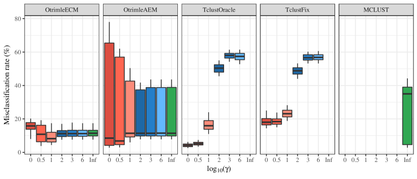
Figure 5: Modified boxplots of the Monte Carlo distribution of misclassification rates for the AsyNoise design: whiskers coincide with (5%, 95%)–quantiles of the distribution.

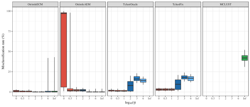
Figure 6: Modified boxplots of the Monte Carlo distribution of misclassification rates for the GEM design: whiskers coincide with (5%, 95%)–quantiles of the distribution.

Results are summarized in Tables 3 and 4, and Figures 5 and 6. Since MCLUST does not enforce an eigenratio constraint, results are recorded at $\gamma=+\infty$, although MCLUST has its own covariance regularization. MCLUST is seriously affected by contamination in both designs, its performance is better for the AsyNoise design for which the boxplot of Figure 5 shows that in some replica it can produce misclassification rates below 10%. Regarding the Otrimle and Tclust versions, the performance depends on the setting of the eigenratio constraint. However, OtrimleECM offers the most stable performance in both designs. OtrimleECM achieves the best misclassification performance in all situations except for few cases where TclustOracle does better, but in fact, TclustOracle is run with the assumption that one knows exactly the expected amount of noise, which is never true in reality. It is worth to note that TclustOracle seems to not tolerate large values of $\gamma$ in both designs. This is counterintuitive at least for GEM, where the true $\log_{10}(\gamma)$ is between 3 and 6, but in this range both TclustOracle and TclustFix have serious problems. OtrimleAEM is the second best overall, although it shows a large positive skewness in the distribution of the misclassification rates for AsyNoise, and in both designs it is not able to enforce low $\gamma$ values appropriately. This is because in OtrimleAEM an approximate eigenratio constraint is applied at the end of the EM iteration, while during the iteration only a minimum determinant condition is controlled. These results show a remarkable improvement of the ECM algorithm 2 over the approximate solution proposed in Coretto and Hennig (2016).

In practice the user has to specify $\gamma$. According to the results shown here, OtrimleECM is not very sensitive to this choice. Also the results show that good misclassification rates can be achieved in GEM, with a true $\gamma>3000$, using a much lower $\gamma$ for ORIMLE; actually for TCLUST a much lower $\gamma$ is even required to achieve good results. Choosing a lower $\gamma$ in such situations may provide some welcome regularization. $\gamma=100$ often seems to be a sensible choice. However, the user needs to have in mind that a straight interpretation of $\gamma$ requires that a variance of 1 (say) along a one-dimensional projection has the same meaning in all directions in data space, which is particularly doubtful if variables have different measurement units or variable-wise variations are not meaningfully comparable. In such cases sphering or at least variable standardization may be advisable.

8 Concluding Remarks

The RIMLE robustifies the MLE in the Gaussian mixture model by adding an improper constant mixture component to catch outliers and points that cannot appropriately assigned to any cluster. Characteristics of the method compared to other robust clustering methods aiming for approximately Gaussian clusters are a smooth mixture-type transition between clusters and noise, and the fact that noise and outliers are not modelled by a specific and usually misspecified distribution, but rather as anything where the estimated mixture density is so low that the observation is rather classified to the constant noise than to any mixture component. If needed, the density value of the improper constant noise component can be chosen in a data-adaptive based on the OTRIMLE criterion developed in (Coretto and Hennig, 2016). The RIMLE/OTRIMLE has shown competitive performance when compared with state of the art methods for robust model-based clustering methods. In this paper we investigated theoretical properties of the RIMLE, and it is shown existence, consistency, breakdown behaviour, and convergence of algorithms. Since the RIMLE coincides with the MLE for Gaussian finite mixture models (when $\delta=0$), the present paper also gives a comprehensive treatment for it which was missing in the literature.

References

- Alexandrovich (2014) Alexandrovich, G. (2014). A note on the article ‘Inference for multivariate normal mixtures’ by J. Chen and X. Tan. J. Multivariate Anal. 129, 245–248.
- Anderson and Olkin (1985) Anderson, T. W. and I. Olkin (1985). Maximum-likelihood estimation of the parameters of a multivariate normal distribution. Linear Algebra Appl. 70, 147–171.
- Banfield and Raftery (1993) Banfield, J. D. and A. E. Raftery (1993). Model-based gaussian and non-gaussian clustering. Biometrics 49, 803–821.
- Bertsekas (1999) Bertsekas, D. P. (1999). Nonlinear Programming. Athena Scientific.
- Chen and Tan (2009) Chen, J. and X. Tan (2009). Inference for multivariate normal mixtures. J. Multivariate Anal. 100(7), 1367–1383.
- Coretto and Hennig (2010) Coretto, P. and C. Hennig (2010). A simulation study to compare robust clustering methods based on mixtures. Advances in Data Analysis and Classification 4(2), 111–135.
- Coretto and Hennig (2011) Coretto, P. and C. Hennig (2011). Maximum likelihood estimation of heterogeneous mixtures of gaussian and uniform distributions. Journal of Statistical Planning and Inference 141(1), 462–473.
- Coretto and Hennig (2016) Coretto, P. and C. Hennig (2016). Robust improper maximum likelihood: tuning, computation, and a comparison with other methods for robust Gaussian clustering. Journal of the American Statistical Association 111, 1648–1659.
- Coretto and Hennig (2017) Coretto, P. and C. Hennig (2017). otrimle: Robust model-based clustering. R package version 1.0. Available at: https://CRAN.R-project.org/package=otrimle.
- Cuesta-Albertos et al. (1997) Cuesta-Albertos, J. A., A. Gordaliza, and C. Matrán (1997). Trimmed k-means: An attempt to robustify quantizers. Annals of Statistics 25, 553–576.
- Dennis (1981) Dennis, J. E. J. (Ed.) (1981). Algorithms for nonlinear fitting, Cambridge, England. NATO advanced Research Symposium: Cambridge University Press.
- Ester et al. (1996) Ester, M., H.-P. Kriegel, J. Sander, and X. Xu (1996). A density-based algorithm for discovering clusters in large spatial databases with noise. In Proceedings of the 2nd International Conference on Knowledge Discovery and Data Mining (KDD-96), pp. 226–231. Institute for Computer Science, University of Munich.
- Fraley (1998) Fraley, C. (1998, jan). Algorithms for model-based gaussian hierarchical clustering. SIAM Journal on Scientific Computing 20(1), 270–281.
- Fraley and Raftery (2002) Fraley, C. and A. E. Raftery (2002). Model-based clustering, discriminant analysis, and density estimation. Journal of the American Statistical Association 97, 611–631.
- Fraley et al. (2012) Fraley, C., A. E. Raftery, T. B. Murphy, and L. Scrucca (2012). mclust version 4 for r: Normal mixture modeling for model-based clustering, classification, and density estimation. Technical Report 597, University of Washington, Department of Statistics.
- Fritz et al. (2012) Fritz, H., L. A. García-Escudero, and A. Mayo-Iscar (2012). tclust: An R package for a trimming approach to cluster analysis. Journal of Statistical Software 47(12), 1–26.
- Fritz et al. (2013) Fritz, H., L. A. García-Escudero, and A. Mayo-Iscar (2013). A fast algorithm for robust constrained clustering. Comput. Statist. Data Anal. 61, 124–136.
- Gallegos (2002) Gallegos, M. T. (2002). Maximum likelihood clustering with outliers. In Classification, Clustering, and Data Analysis, pp. 247–255. Springer.
- Gallegos and Ritter (2005) Gallegos, M. T. and G. Ritter (2005). A robust method for cluster analysis. Annals of Statistics 33(5), 347–380.
- Gallegos and Ritter (2009) Gallegos, M. T. and G. Ritter (2009). Trimmed ML estimation of contaminated mixtures. Sankhya (Ser. A) 71, 164–220.
- Gallegos and Ritter (2013) Gallegos, M. T. and G. Ritter (2013). Strong consistency of -parameters clustering. Journal of Multivariate Analysis 117, 14–31.
- García-Escudero and Gordaliza (1999) García-Escudero, L. A. and A. Gordaliza (1999). Robustness properties of -means and trimmed -means. Journal of the American Statistical Association 94, 956–969.
- García-Escudero et al. (2008) García-Escudero, L. A., A. Gordaliza, C. Matrán, and A. Mayo-Iscar (2008). A general trimming approach to robust cluster analysis. Annals of Statistics 38(3), 1324–1345.
- García-Escudero et al. (2014) García-Escudero, L. A., A. Gordaliza, C. Matrán, and A. Mayo-Iscar (2014). Avoiding spurious local maximizers in mixture modeling. Statistics and Computing 25, 1–15.
- García-Escudero et al. (2015) García-Escudero, L. A., A. Gordaliza, C. Matrán, A. Mayo-Iscar, and C. Hennig (2015). Robustness and outliers. In C. Hennig, M. Meila, F. Murtagh, and R. Rocci (Eds.), Handbook of Cluster Analysis, pp. 653–678. Boca Raton FL: CRC Press.
- Gavish and Donoho (2017) Gavish, M. and D. L. Donoho (2017). Optimal shrinkage of singular values. IEEE Transactions on Information Theory 63(4), 2137–2152.
- Hahsler (2016) Hahsler, M. (2016). dbscan: Density Based Clustering of Applications with Noise (DBSCAN) and Related Algorithms. R package version 0.9-7.
- Hathaway (1985) Hathaway, R. J. (1985). A constrained formulation of maximum-likelihood estimation for normal mixture distributions. The Annals of Statistics 13, 795–800.
- Hennig (2004) Hennig, C. (2004). Breakdown points for maximum likelihood estimators of location-scale mixtures. The Annals of Statistics 32(4), 1313–1340.
- Hennig (2008) Hennig, C. (2008). Dissolution point and isolation robustness: robustness criteria for general cluster analysis methods. Journal of Multivariate Analysis 99, 1154–1176.
- Hennig (2015a) Hennig, C. (2015a). Clustering strategy and method selection. In C. Hennig, M. Meila, F. Murtagh, and R. Rocci (Eds.), Handbook of Cluster Analysis, Chapter 31, pp. 703–730. Chapman & Hall/CRC, Boca Raton FL.
- Hennig (2015b) Hennig, C. (2015b). What are the true clusters? Pattern Recognition Letters 64, 53–62.
- Hennig and Liao (2013) Hennig, C. and T. F. Liao (2013). How to find an appropriate clustering for mixed type variables with application to socioeconomic stratification (with discussion). Journal of the Royal Statistical Science, Series C (Applied Statistics) 62, 309–369.
- Ingrassia (2004) Ingrassia, S. (2004). A likelihood-based constrained algorithm for multivariate normal mixture models. Statistical Methods & Applications 13(2), 151–166.
- Ingrassia and Rocci (2007) Ingrassia, S. and R. Rocci (2007). Constrained monotone EM algorithms for finite mixture of multivariate gaussians. Computational Statistics and Data Analysis 51, 5339–5351.
- Ingrassia and Rocci (2011) Ingrassia, S. and R. Rocci (2011). Degeneracy of the EM algorithm for the MLE of multivariate gaussian mixtures and dynamic constraints. Computational statistics & data analysis 55(4), 1715–1725.
- Jennrich (1969) Jennrich, R. I. (1969). Asymptotic properties of non-linear least squares estimators. Annals of Mathematical Statistics 40, 633–643.
- Kiefer (1953) Kiefer, J. (1953). Sequential minimax search for a maximum. Proceedings of the American Mathematical Society 4(3), 502–506.
- Kiefer and Wolfowitz (1956) Kiefer, N. M. and J. Wolfowitz (1956). Consistency of the maximum likelihood estimation in the presence of infinitely many incidental parameter. Annals of Mathematical Statistics 27(364), 887–906.
- McLachlan and Peel (2000) McLachlan, G. J. and D. Peel (2000). Robust mixture modelling using the t–distribution. Statistics and Computing 10(4), 339–348.
- Meng and Rubin (1993) Meng, X.-L. and D. B. Rubin (1993). Maximum likelihood estimation via the ECM algorithm: a general framework. Biometrika 80(2), 267–278.
- Redner (1981) Redner, R. (1981). Note on the consistency of the maximum likelihood estimate for nonidentifiable distributions. The Annals of Statistics 9, 225–228.
- Redner and Walker (1984) Redner, R. A. and H. F. Walker (1984). Mixture densities, maximum likelihood and the EM algorithm. SIAM Review 26, 195–239.
- Ritter (2014) Ritter, G. (2014). Robust Cluster Analysis and Variable Selection. Monographs on Statistics and Applied Probability. Chapman and Hall/CRC.
- Theobald (1975) Theobald, C. (1975). An inequality with application to multivariate analysis. Biometrika 62(2), 461–466.
- Van der Vaart (2000) Van der Vaart, A. W. (2000). Asymptotic statistics, Volume 3. Cambridge university press.
- van der Vaart and Wellner (1996) van der Vaart, A. W. and J. A. Wellner (1996). Weak Convergence and Empirical Processes. New York: Springer.
- Won et al. (2013) Won, J.-H., J. Lim, S.-J. Kim, and B. Rajaratnam (2013). Condition-number-regularized covariance estimation. J. R. Stat. Soc. Ser. B. Stat. Methodol. 75(3), 427–450.
- Wu (1983) Wu, C. F. J. (1983). On the convergence properties of the EM algorithm. Annals of Statistics 11(1), 95–103.