Asymptotic Properties of Unbounded Quadrature Domains the Plane

Abstract.

We prove that if $\Omega$ is a simply connected quadrature domain of a distribution with compact support and the infinity point belongs the boundary, then the boundary has an asymptotic curve that is a straight line or a parabola or an infinite ray. In other words, such quadrature domains in the plane are perturbations of null quadrature domains.

1. Introduction

A domain $\Omega$ in the complex plane ${\mathord{\mathbb{C}}}$ is called a quadrature domain (QD) of a measure $\mu$ (or a distribution) and for the class of analytic functions, if $\mu_{\mid_{{\mathord{\mathbb{C}}}\setminus\Omega}}=0$ and

(1.1) $$\int_{\Omega}fdA=\mu(f)\quad\text{for all}\ f\in AL^{1}(\Omega).$$

Here $AL^{1}(\Omega)$ is the space of all analytic and integrable functions in $\Omega$ and $dA$ the area measure. We may also consider quadrature domains for the class of harmonic functions. In that case the space $AL^{1}(\Omega)$ is replaced by $HL^{1}(\Omega)$, the set of all harmonic and integrable functions in $\Omega$, and the measure $\mu$ is real. Any QD for the class of harmonic functions is also a QD for the class of analytic functions.

A particular class of unbounded QDs is the family of null quadrature domains, that is, domains $\Omega$ for which

$$\int_{\Omega}fdA=0,\quad\text{for all}\ f\in AL^{1}(\Omega).$$

This class comprises half-planes, the exteriors of parabolas, ellipses and strips, and the complement of any set which contains more than three points and lies in a straight line [16].

The main result of the present paper asserts that if $\Omega$ is a simply connected QD of a measure with compact support and with an unbounded boundary, then $\Omega$ is asymptotically like a null QD. More precisely, the boundary of $\Omega$, $\partial\Omega$, has an asymptotic curve that is either a straight line or a parabola or an infinite ray.

In terms of free boundary problems this result has the following interpretation. Let $\chi_{\Omega}$ denotes the characteristic set of $\Omega$ and assume there is a solution to the overdetermined problem

$$\left\{\begin{array}[]{ll}\Delta u=\chi_{\Omega}-g\ \ \text{in}&{\mathord{\mathbb{R}}}^{2}\\ u=|\nabla u|=0\ \ \text{on}&{\mathord{\mathbb{R}}}^{2}\setminus\Omega,\end{array}\right.$$

where $g$ has a compact support in $\Omega$, and that the boundary of $\Omega$ is unbounded. Then $\partial\Omega$ has an asymptotic curve as is described above.

Unbounded QDs in the two dimensional plane were studied by Sakai [17, 19], Shapiro [22], and recently by Lee and Makarov [13]. Sakai showed that for a given non–negative measure with compact support there is an unbounded QD that contains a given null QD [17, Ch. 11]. He used variational methods that are also available in higher dimensions. Shapiro proposed the use of an inversion in order to characterize unbounded quadrature domains [22]. This idea was accomplished by Sakai in [19]. However, the asymptotic behavior of the boundary were not considered in those papers.

Our results are inspired by the study of contact surfaces, and in particular by the works of Strakhov [23, 24], since in those works the asymptotic line appears naturally. These problems arise in geophysics and in the two dimensional plane they have the following formulation. Assume that an unbounded Jordan curve $\Gamma$ separates an infinite strip into two domains with different constant densities. Assume also that the strip is parallel to the $x$–axis. Strakhov showed that if $\Gamma$ has an asymptotic line ${\rm Im}(z)=h$ ($z=x+iy$), then the gravitational fields can be computed by the Cauchy integral

(1.2) $$\int_{\Gamma}\sigma\frac{\bar{w}-w+2ih}{w-z}dw,$$

where $\sigma$ is the difference between the two densities and $z$ lies above the strip. The question is whether the shape of $\Gamma$ can be determined by the Cauchy integral when ${\rm Im}(z)$ is large.

This type of problem is embedded in the frame of inverse problems in potential theory, in which one aims to determinate the shape of a body from the measurements of its Newtonian potential far away from the body itself [5, 9, 10, 15, 26]. Quadrature domains are closely related to these problems [7, 14], for example, in the two dimensional plane the Schwarz function has a significant role in all these types of problems [1, 3, 21, 25].

An essential tool of the proof is the relation between the conformal mapping in lower half–plane and the Cauchy transform of the measure $\mu$ of the QD (formula (2.15)). Conformal mappings have been frequently incorporated in all these types of problems. The main feature of these sorts of results is to asserts that a conformal map from the unit disk to a domain $\Omega$ is rational if and only if $\Omega$ is a QD of a combination of Dirac measures and their derivatives [1, 3, 6], or equivalently, the complex derivative of the external logarithmic potential of $\chi_{\Omega}$ is a rational function [10, 24, 25].

Strakhov used the specific form of the conformal mapping in the lower half-plane (see (2.4) and (2.5)) in order to show that contact surfaces are highly non-unique [24]. Moreover, he constructed a continuous family of third order algebraic curves such that the Cauchy integral (1.2) has the same value for all the curves in the family when ${\rm Im}(z)$ is large. In the context of QDs, Strakhov’s example provides an explicit family of unbounded domains, and each one of them is a QD of the same Dirac measure. Furthermore, the domains in the family converge to a union of a disk and a half–plane, in other words, a union of a disk and a null QD. We will extend Strakhov’s example to other types of null QDs, that is, we will construct families of unbounded QDs of a fixed Dirac measure, and such that their boundary has a parabola, or an infinite ray, as an asymptotic curve.

We believe that the structure of unbounded QDs in higher dimension is similar to the two dimensional. However, the corresponding theory in higher dimensions is very restricted, and most of the problems are open. For example, in [12] it is proved that if $\Omega\subset{\mathord{\mathbb{R}}}^{n}$ is an unbounded QD of a measure with compact support and the complement of $\Omega$ is not too thin at infinity, then inversion of the boundary is a $C^{1}$ surface near the origin. However, this does not imply that the boundary has an asymptotic plane. For further properties of unbounded QDs in higher dimensions see [11, 20].

The plan of the paper is the following: In the next section we shall first establish the relation between rational conformal mappings in the lower half–plane and quadrature identities. Having established that, the main result follows easily. Section 3 deals with contact surfaces. Although Strakhov’s model is published in [23], we shall present its basic idea here, and in particular, we will emphasize its connections to unbounded QDs. In Section 4 we shall construct examples of families of unbounded QDs of a fixed Dirac measure, and in each example the boundary has a different type of an asymptotic curve.

Throughout this paper $f^{\ast}$ stands for $\bar{f}(\bar{z})$ and $\chi_{\Omega}$ is the characteristic function of a set $\Omega$. We also may assume that $\Omega$ is the interior of its closure whenever it is a QD (see cf. [11, Corollary 2.15]).

2. Conformal mappings and quadrature domains

Conformal mappings have been used extensively in QDs and the inverse problem of potential theory. A fundamental property is the relations between the conformal mapping, quadrature identity (1.1) and the Cauchy transform. To be more specific, a conformal map from the unit disk to a domain $\Omega$ is rational if and only if $\Omega$ is a QD of a combination of Dirac measures and their derivatives [1, 3, 6], or equivalently, the Cauchy transform of the measure $\chi_{\Omega}$ is a rational function outside $\Omega$ [10, 25].

Theorem 2.1 below comprises similar statements. It was proved in the context of contact surfaces under the assumption that the boundary has an asymptotic line [4, 24], and for QDs by Shapiro under the assumption that the Schwarz function $S(z)$ tends to infinity as $z$ goes to infinity [22]. Shapiro used that assumption in order to apply an inversion and to reduce the problem to the one of bounded QDs. This assumption was affirmed later by Sakai in [19]. Since the proof of Theorem 2.1 is the core for the main result we prove it here. We also slightly extend these previous results, and in addition, our proof is based upon the generalized Cauchy transform.

Let $z$ and $\zeta$ be points in the complex plane. For a measure $\mu$, we denote by ${\mathord{\mathcal{C}}}^{\mu}$ the Cauchy transform of $\mu$,

(2.1) $${\mathord{\mathcal{C}}}^{\mu}(z):=\dfrac{1}{\pi}\int\dfrac{d\mu(\zeta)}{\zeta-z}.$$

Whenever $\sigma\in L^{\infty}({\mathord{\mathbb{C}}})$ and $\mu=\sigma\chi_{D}dA$ we will denote the Cauchy transform by $C^{\sigma D}$.

The Cauchy transform satisfies the differential equation $\partial_{\bar{z}}\mathcal{C}^{\mu}=-\mu$ in the distributional sense, and it is well defined whenever $\mu$ has a compact support. But it may not converge when the measure has arbitrary support. In order to over come this we use the following device that was first implemented by Bers [2] and later by Sakai [16, 19].

We modify the Cauchy kernel $(\pi(\zeta-z))^{-1}$ by

(2.2) $$\mathcal{K}(\zeta,z,a,b)=\dfrac{1}{\pi}\left(\dfrac{1}{\zeta-z}+\dfrac{z-b}{(b-a)(\zeta-a)}+\dfrac{z-a}{(a-b)(\zeta-b)}\right),\quad a\neq b.$$

Since $\mathcal{K}(\zeta,z,a,b)=O(|\zeta|^{-3})$ for large $|\zeta|$, the integral

(2.3) $$\mathcal{C}^{g}_{\mathcal{K}}(z)=\int\mathcal{K}(\zeta,z,a,b)g(\zeta)dA(\zeta),$$

converges for any $g\in L^{\infty}({\mathord{\mathbb{C}}})$. The transformation (2.3) is called a generalized Cauchy transform of $g$. Obviously if ${a,b}\not\in{\rm supp}(g)$, then $\partial_{\bar{z}}\mathcal{C}^{g}_{\mathcal{K}}=-g$.

Let $\mathbb{H}_{\pm}$ denote the upper/lower half-plane respectively and consider a conformal map $\psi$, from $\mathbb{H}_{-}$ onto a domain $\Omega$ of, the form

(2.4) $$z=\psi(w)=q(w)+\varphi(w),$$

where $q$ is a quadratic polynomial,

(2.5) $$\varphi(w)=\sum_{k=1}^{m}\sum_{j=0}^{m_{k}}\dfrac{a_{kj}}{(w-b_{k})^{j+1}}+\sum_{k=1}^{n}c_{k}\int_{d_{k}}^{d_{k+1}}\dfrac{1}{w-s}ds,\{b_{1},\ldots,b_{m},d_{1},\ldots,d_{n+1}\}\subset\mathbb{H}_{+}$$

and $\{a_{kj}\}$, $\{c_{k}\}$ are complex numbers. The integrals are along piecewise straight lines connecting $d_{k}$ to $d_{k+1}$ and do not pass through the points $b_{k}$. We assume that the points $\{b_{k}\}_{k=1}^{m},\{d_{k}\}_{k=1}^{n+1}$ are distinct.

For given points $\{\beta_{1},\ldots,\beta_{m}\}$ and $\{\delta_{1},\ldots,\delta_{n+1}\}$, we define a distribution $T$ as follows:

(2.6) $$T\left(\phi\right)=\sum_{k=1}^{m}\sum_{j=0}^{m_{k}}\alpha_{kj}\partial_{z}^{j}\phi(\beta_{k})+\sum_{k=1}^{n}\bar{c}_{k}\int_{\delta_{k}}^{\delta_{k+1}}\phi(s)ds,$$

where the integrals are along piecewise straight lines connecting $\delta_{k}$ to $\delta_{k+1}$, $\alpha_{kj}$ and $c_{k}$ are constants. The test function $\phi$ belongs to $C^{\infty}(D)$, for any open set $D$ such that $\mathop{\mathrm{supp}}(T)\subset D$.

Theorem 2.1.

Let $\Omega$ be a simply connected domain with an unbounded boundary $\partial\Omega$. Then the following are equivalent:

1. The domain $\Omega$ is QD of a distribution $T$ of the form (2.6), that is,

   (1.1) $$\int_{\Omega}fdA=T(f)\qquad\text{for all}\ f\in AL^{1}(\Omega).$$

2. There is a conformal map $\psi$ from $\mathbb{H}_{-}$ onto $\Omega$ of the form (2.4)–(2.5).

Remark 2.2.

The relations between the coefficients of the conformal mapping $\psi$ and the distribution $T$ are as follows: $\beta_{k}=\psi(\bar{b}_{k})$, $\delta_{k}=\psi(\bar{d}_{k})$ and $\{\alpha_{kj}\}$ are depended on $\{a_{kj}\}$ through equation (2.8) below.

Proof( of Theorem 2.1). Suppose first that $\Omega=\psi(\mathbb{H}_{-})$, where $\psi$ is a conformal mapping of the form (2.4)–(2.5). Since the class consisting of holomorphic functions $f$ in a neighborhood of $\Omega$ such that $f(z)=O(|z|^{-k})$ at infinity is dense in $AL^{1}(\Omega)$ for any integer $k\geq 3$ (see [8, 22]), we may prove the identity (2.6) for $f$ that is holomorphic in a neighborhood of $\Omega$ and has arbitrary polynomial decay at infinity.

Let $B_{r}$ be a ball with radius $r$ and center at the origin, and let $\Omega_{r}$ be the image of $\mathbb{H}_{-}\cap B_{r}$ under the map $\psi$. Then by Green’s theorem,

$$\begin{split}\int\limits_{\Omega_{r}}fdA&=\frac{1}{2i}\int\limits_{\partial\Omega_{r}}\bar{z}f(z)dz=\frac{1}{2i}\int\limits_{-r}^{r}\overline{\psi(t)}f(\psi(t))\psi^{\prime}(t)dt\\ &+\frac{1}{2i}\int\limits_{\{|w|=r,{\rm Im}(w)<0\}}\overline{\psi(w)}f(\psi(w))\psi^{\prime}(w)dw.\end{split}$$

Noting that $\psi$ has at most a quadratic growth at infinity and $f$ has arbitrary polynomial decay, the second integral of the right hand side tends to zero as $r$ goes to infinity. Hence

(2.7) $$\int\limits_{\Omega}fdA=\frac{1}{2i}\int\limits_{-\infty}^{\infty}\overline{\psi(t)}f(\psi(t))\psi^{\prime}(t)dt.$$

Let $\overline{\psi(\bar{w})}=\psi^{\ast}(w)$. Since $\psi^{\ast}(t)=\overline{\psi}(t)$ for $t\in{\mathord{\mathbb{R}}}$, we may replace $\overline{\psi}$ by $\psi^{\ast}$ in (2.7). Note $\psi^{\ast}=q^{\ast}+\varphi^{\ast}$ is holomorphic outside the reflection of the singularities of $\varphi$, and since $f$ has polynomial decay at infinity we have that

$$\lim_{r\to\infty}\int\limits_{\{|w|=r,{\rm Im}(w)<0\}}{\psi^{\ast}(w)}f(\psi(w))\psi^{\prime}(w)dw=0.$$

Hence, we can replace the line integral in (2.7) by several line integrals around the singularities of $\varphi^{*}$ in $\mathbb{H}_{-}$. Let $C_{\rho}(\bar{b}_{k})$ be a small circle around $\bar{b}_{k}$, then

(2.8) $$\begin{split}&\dfrac{1}{2i}\int\limits_{C_{\rho}(\bar{b}_{k})}\left(q^{*}(w)+\varphi^{*}(w)\right)f(\psi(w))\psi^{\prime}(w)dw\\ =&\dfrac{1}{2i}\sum_{j=0}^{m_{k}}\int\limits_{C_{\rho}(\bar{b}_{k})}\left(\dfrac{\bar{a}_{kj}}{(w-\bar{b}_{k})^{j+1}}\right)f(\psi(w))\psi^{\prime}(w)dw\\ =&\pi\sum_{j=0}^{m_{k}}\bar{a}_{kj}{\rm Res}\left(\dfrac{(f\circ\psi)\psi^{\prime}}{(w-\bar{b}_{k})^{j+1}},\bar{b}_{k}\right)=:\sum_{j=0}^{m_{k}}\alpha_{kj}\partial_{z}^{j}f(\beta_{k}),\end{split}$$

where $\beta_{k}=\psi(\bar{b}_{k})$.

Let $\gamma$ be a closed curve in $\mathbb{H}_{-}$ around the polygonal curve connecting $\bar{d}_{1}$ to $\bar{d}_{n+1}$, and such that it does not surround any of the points $\bar{b}_{i},i=1,\ldots,m$. Then

$$\begin{split}&\dfrac{1}{2i}\int\limits_{\gamma}\left(q^{*}(w)+\varphi^{*}(w)\right)f(\psi(w))\psi^{\prime}(w)dw\\ =&\dfrac{1}{2i}\int\limits_{\gamma}\left(\sum_{k=1}^{n}\bar{c}_{k}\int_{\bar{d}_{k}}^{\bar{d}_{k+1}}\dfrac{1}{w-s}ds\right)f(\psi(w))\psi^{\prime}(w)dw\\ =&\dfrac{1}{2i}\sum_{k=1}^{n}\bar{c}_{k}\int_{\bar{d}_{k}}^{\bar{d}_{k+1}}\left(\int\limits_{\gamma}\dfrac{1}{w-s}f(\psi(w))\psi^{\prime}(w)dw\right)ds\\ =&\pi\sum_{k=1}^{n}\bar{c}_{k}\int_{\bar{d}_{k}}^{\bar{d}_{k+1}}f(\psi(s))\psi^{\prime}(s)ds=\pi\sum_{k=1}^{n}\bar{c}_{k}\int_{\delta_{k}}^{\delta_{k+1}}f(\tau)d\tau,\end{split}$$

where $\delta_{k}=\psi(\bar{d}_{k})$. Summing all the integrals around the singularities of $\varphi^{\ast}$ in $\mathbb{H}_{-}$, we obtain the quadrature identity (1.1) with $T$ as in (2.6).

For the converse assertion we follow Aharonov and Shapiro method [1] with some obvious modifications, and we shall also use Sakai’s regularity results [18, 19] to overcome the difficulty near the infinity point.

Calculating the generalized Cauchy transform of the distribution $T$, we find that

(2.9) $$\mathcal{C}_{\mathcal{K}}^{T}(z)=\dfrac{1}{\pi}\sum_{k=1}^{m}\sum_{j=0}^{m_{k}}\frac{(-1)^{j}j!\alpha_{kj}}{\left(z-\beta_{k}\right)^{j+1}}+\dfrac{1}{\pi}\sum_{k=1}^{n}\bar{c}_{k}\int_{\delta_{k}}^{\delta_{k+1}}\dfrac{1}{s-z}ds+L(z),$$

where $L(z)$ is a linear function. Let $a,b\not\in\Omega$. Then for any $z\not\in\Omega$ the modified Cauchy kernel $\mathcal{K}(\cdot,z,a,b)$ belongs to $AL^{1}(\Omega)$. Hence, the quadrature identity (1.1) implies that $\mathcal{C}_{\mathcal{K}}^{\Omega}(z)=\mathcal{C}_{\mathcal{K}}^{T}(z)$ for $z\not\in\Omega$. Since $\mathcal{C}_{\mathcal{K}}^{T}(z)$ is analytic for $z$ outside the support of $T$, and $\mathop{\mathrm{supp}}(T)\Subset\Omega$,

$$S(z)=\bar{z}+\mathcal{C}_{\mathcal{K}}^{\Omega}(z)-\mathcal{C}_{\mathcal{K}}^{T}(z)$$

is the Schwarz function of the boundary $\partial\Omega$ in $\Omega$. That is, $S(z)=\bar{z}$ on $\partial\Omega$ and it is holomorphic for $z\in\Omega$ near $\partial\Omega$.

Let now $\psi$ be a conformal map from $\mathbb{H}_{-}$ to $\Omega$ and set

(2.10) $$F(w)=\left\{\begin{array}[]{ll}S(\psi(w)),&w\in\mathbb{H}_{-}\\ \psi^{*}(w),&w\in\mathbb{H}_{+}\end{array}\right..$$

Since $S(\psi(t))=\overline{\psi(t)}=\psi^{\ast}(t)$ for $t\in{\mathord{\mathbb{R}}}$, the function $F$ is analytically continuable to a single-valued function across the real line (here we rely of Sakai’s regularity result that implies that the boundary is a union of piecewise analytic arcs [18]). The crucial point is the analytic continuation near infinity. In order to overcome this difficulty we use an inversion, we set $\Omega_{\rm inv}=\{z:1/{z}\in\Omega\}$ and $\partial\Omega_{\rm inv}=\{z:1/z\in\partial\Omega\}$. Then it follows from Sakai’s regularity result [19, Corollary 2.6], that

$$S_{\rm inv}(z):=\left\{\begin{array}[]{ll}\frac{1}{S({z}^{-1})},&z\neq 0\\ 0,&z=0\end{array}\right.$$

is the Schwarz function of $\partial\Omega_{\rm inv}$. Let $\Psi(\zeta):=1/\psi(-\zeta^{-1})$ and set

$$\widetilde{F}(\zeta)=\left\{\begin{array}[]{ll}S_{\rm inv}(\Psi(\zeta)),&\zeta\in\mathbb{H}_{-}\\ \Psi^{*}(\zeta),&\zeta\in\mathbb{H}_{+}\end{array}\right..$$

Then the function $\Psi(\zeta)$ maps $\mathbb{H}_{-}$ conformally onto $\Omega_{\rm inv}$ and $S_{\rm inv}(\Psi(t))=\overline{\Psi(t)}$ for $t$ in ${\mathord{\mathbb{R}}}$. Hence $\widetilde{F}$ has an analytic continuation across the real line, and in particular, in a neighborhood of the origin. Thus $F$ in (2.10) is holomorphic in a neighborhood of infinity.

Let $\{\bar{b}_{1},\ldots,\bar{b}_{m},\bar{d}_{1},\ldots,\bar{d}_{n+1}\}\subset\mathbb{H}_{-}$ be the pre-image of $\{\beta_{1},\ldots,\beta_{m}\}$ and $\{\delta_{1},\ldots,\delta_{n+1}\}$ under $\psi$. From (2.9) and (2.10) we see that $F^{\prime}(w)$ is a single-valued meromorphic function in the Riemann sphere with poles of order higher than or equal to two at the points $\{\bar{b}_{1},\ldots,\bar{b}_{m}\}$, and of order one at the points $\{\bar{d}_{1},\ldots,\bar{d}_{n+1}\}$. Since $\psi$ is univalent in $\mathbb{H}_{-}$, $F$ has polynomial growth at infinity, and hence $F$ is a meromorphic function in the entire plane of the form

(2.11) $$F(w)=q^{\ast}(w)+\sum_{k=1}^{n}\sum_{j=0}^{m_{k}}\dfrac{\bar{a}_{kj}}{(w-\bar{b}_{k})^{j+1}}+\sum_{k=1}^{n+1}\gamma_{k}\log(w-\bar{d}_{k}),$$

where $q$ is a polynomial and $a_{kj},\gamma_{k}$ are constants. From (2.10) we see that $F$ is a single–valued function and hence $\sum_{k=1}^{n+1}\gamma_{k}\log(w-\bar{d}_{k})$ is also a single-valued. This implies that $\sum_{k=1}^{n+1}\gamma_{k}=0$, and

(2.12) $$\sum_{k=1}^{n+1}\gamma_{k}\log(w-\bar{d}_{k})=\sum_{k=1}^{n}\bar{c}_{k}\int_{\bar{d}_{k}}^{\bar{d}_{k+1}}\dfrac{1}{w-s}ds$$

for some constants $\{c_{k}\}$ (see Remark 2.4 below). Setting

$$\varphi^{*}(w)=\sum_{k=1}^{m}\sum_{j=0}^{m_{k}}\dfrac{\bar{a}_{kj}}{(w-\bar{b}_{k})^{j+1}}+\sum_{k=1}^{n}\bar{c}_{k}\int_{\bar{d}_{k}}^{\bar{d}_{k+1}}\dfrac{1}{w-s}ds,$$

we see from (2.10), (2.11) and (2.12) that

$$\psi(w)=q(w)+\varphi(w),$$

where $\varphi$ is given by (2.5).

It remains to prove that the degree of $q$ does not exceed two. Let $N$ be the degree of $q$, then we may write $\psi(w)=Aw^{N}g(w)$, where $g$ is holomorphic in $\mathbb{H}_{-}$ and $g(\infty)=1$. Therefore $\Psi(\zeta):=1/\psi(-\zeta^{-1})={(-\zeta)^{N}}{\left(Ag(-\zeta^{-1})\right)}^{-1}$. Now, according to Sakai’s regularity result [18, 19], there are three possibilities: Either $\partial\Omega_{\rm inv}$ is a smooth analytic curve near the origin, or $\partial\Omega_{\rm inv}$ is a union of two tangential analytic arcs in a neighborhood of the origin, or $\partial\Omega_{\rm inv}$ has cusp singularity at the origin. In the first and second cases, $\Psi(t)$ is a smooth curve for $t\in(-\epsilon,\epsilon)$ and some positive $\epsilon$. Then clearly $N=1$. In the third one $\Psi$ has a Taylor expansion $\kappa\left(\zeta^{2}+a_{3}\zeta^{3}+\cdots\right)$, for $\zeta\in\mathbb{H}_{-}\cap\{|\zeta|<\epsilon\}$ and $\kappa\in{\mathord{\mathbb{C}}}$. Then obviously $N=2$. So we conclude that

(2.13) $$q(w)=A_{2}w^{2}+A_{1}w+A_{0}$$

for some complex numbers $A_{2},A_{1}$ and $A_{0}$, and this completes the proof. $\square$

The boundary of $\Omega$, $\partial\Omega$, has a parametric representation $\{\psi(t)=q(t)+\varphi(t):t\in{\mathord{\mathbb{R}}}\}$. Since $\lim_{t\to\pm\infty}\varphi(t)=0$, $\partial\Omega$ has the asymptotic of the curve $\{q(t):t\in{\mathord{\mathbb{R}}}\}$. Hence there are three possibilities of asymptotic curves: In case $A_{2}=0$ in (2.13), then $\partial\Omega$ has an asymptotic of a straight line. Or else, we may write

$$q(w)=A_{2}\left(w^{2}+\frac{A_{1}}{A_{2}}w+\frac{A_{0}}{A_{2}}\right).$$

So if ${\rm Im}({A_{1}}/{A_{2}})\neq 0$, then $\partial\Omega$ has an asymptotic of a parabola, otherwise it has an asymptotic of a ray.

This phenomenon of the asymptotic behavior can be extended for unbounded QDs for any distribution with compact support.

Theorem 2.3.

Let $\Omega$ be a simply connected quadrature domain of a distribution $T$ with compact support in $\Omega$. If $\infty\in\partial\Omega$, then the boundary $\partial\Omega$ has an asymptotic curve that is either a straight line or a parabola or an infinite ray.

Proof.

We may assume that the distribution $T$ can be represented by a smooth function $\rho$ with compact support in $\Omega$, that is, $T(\phi)=\int\phi(z)\rho(z)dA$ (see e.g. [21, Lemma 4.3]). Since $\mathcal{C}_{\mathcal{K}}^{\Omega}(z)=\mathcal{C}_{\mathcal{K}}^{\rho}(z)$ for $z\in{\mathord{\mathbb{C}}}\setminus\Omega$,

$$S(z)=\bar{z}+\mathcal{C}_{\mathcal{K}}^{\Omega}(z)-\mathcal{C}_{\mathcal{K}}^{\rho}(z)$$

is the Schwarz function of $\partial\Omega$ when $z\in\Omega$. Similarly to the above proof, we denote by $\psi$ the conformal map from the lower half-plane $\mathbb{H}_{-}$ onto $\Omega$ and define $F$ as in (2.10). Obviously $F(w)$ is holomorphic in the upper half-plane $\mathbb{H}_{+}$, while for $w\in\mathbb{H}_{-}$ we have that

(2.14) $$\begin{split}\partial_{\bar{w}}F(w)&=\overline{\partial_{w}\psi(w)}+\left\{-\chi_{\Omega}\left(\psi(w)\right)+\rho\left(\psi(w)\right)\right\}\overline{\partial_{w}\psi(w)}\\ &=\rho\left(\psi(w)\right)\overline{\partial_{w}\psi(w)}.\end{split}$$

Hence $F$ is holomorphic in $\mathbb{H}_{-}$ apart from the preimage of ${\rm supp}(\rho)$. Since $S(\psi(t))=\overline{\psi(t)}=\psi^{\ast}(t)$ for $t\in{\mathord{\mathbb{R}}}$, $F$ has a holomorphic continuation through the real line.

We now set $\mu=\left(\rho\circ\psi\right)\overline{{\partial_{w}\psi}}$. Then $\left\{\mathcal{C}^{\mu}(w)-\left(\mathcal{C}^{\rho}\left(\psi(w)\right)\right)\right\}$ is a holomorphic function in the lower half–plane. This means that the Cauchy transform $\mathcal{C}^{\mu}$ captures the singularities of $F$. Using inversion as in the proof of Theorem 2.1, we conclude that $F$ is holomorphic near the infinity point, and hence in the Riemann sphere excluding the support of $\mu$. Therfore

$$F(w)=q^{\ast}(w)+\mathcal{C}^{\mu}(w),$$

where $q$ is a polynomial. So by (2.10),

$$\psi(w)=q(w)+\left(\mathcal{C}^{\mu}(w)\right)^{\ast}.$$

Applying again Sakai’s [18, 19] in a similar manner as we did in the previous proof, we obtain that the degree of $q$ is at most two.

Let $K\subset\mathbb{H}_{-}$ denote the support of $\rho\circ\psi$, which is the preimage of $\mathop{\mathrm{supp}}(\rho)$. Then obviously ${\rm supp}(\mu)=K$,

$$\left(\mathcal{C}^{\mu}(w)\right)^{\ast}=\frac{1}{\pi}\overline{\int\frac{\mu(\zeta)}{\bar{w}-\zeta}dA(\zeta)}=\frac{1}{\pi}\int\frac{\overline{\mu}(\bar{\zeta})}{w-\zeta}dA(\zeta)=\mathcal{C}^{\mu^{\ast}}(w),$$

and ${\mathop{\mathrm{supp}}}(\mu^{\ast})=K^{\ast}\subset\mathbb{H}_{+}$, where $K^{\ast}$ is the mirror image of $K$. Thus the conformal map $\psi$ is holomorphic in $\mathbb{H}_{-}$ and satisfies the equation

(2.15) $$\psi(w)=q(w)+\frac{1}{\pi}\int\frac{\mu^{\ast}\left(\zeta\right)}{w-\zeta}dA(\zeta).$$

The boundary $\partial\Omega$ has a parametric representation $\{\psi(t):t\in{\mathord{\mathbb{R}}}\}$. So since $\mathop{\mathrm{supp}}(\mu^{\ast})=K^{\ast}$ is compact, we obtain from (2.15) that

$$\lim_{t\to\pm\infty}\left\{\psi(t)-q(t)\right\}=0.$$

Thus the asymptotic curve is determined by the coefficients of $q$ in (2.13): A straight line if $A_{2}=0$; otherwise, a parabola when ${\rm Im}({A_{1}}/{A_{2}})\neq 0$ and an infinite ray when ${\rm Im}({A_{1}}/{A_{2}})=0$. ∎

Remark 2.4.

Here is a simple argument showing that $\sum_{k=1}^{n+1}\gamma_{k}\log(w-d_{k})$ is single–valued outside the piecewise straight line connected the points $\{d_{1},\ldots,d_{n+1}\}$ if and only if $\sum\gamma_{k}=0$.

Let $\sigma=\sum_{k=1}^{n+1}\gamma_{k}$. Then

$$\begin{split}&\sum_{k=1}^{n+1}\gamma_{k}\log(w-d_{k})\\ =&\sum_{k=1}^{n}\gamma_{k}\log(w-d_{k})+\left\{-(\gamma_{1}+\cdots+\gamma_{n})+\sigma\right\}\log(w-d_{n+1})\\ =&\gamma_{1}\int_{d_{1}}^{d_{2}}\dfrac{1}{w-s}ds+(\gamma_{1}+\gamma_{2})\int_{d_{2}}^{d_{3}}\dfrac{1}{w-s}ds\\ &+\cdots+(\gamma_{1}+\cdots+\gamma_{n})\int_{d_{n}}^{d_{n+1}}\dfrac{1}{w-s}ds+\sigma\log(w-d_{n+1}).\end{split}$$

Since the integrals are holomorphic off the curve, while $\log(w-d_{n+1})$ is not single–valued in any neighborhood of $d_{n+1}$, we see that $\sum_{k=1}^{n+1}\gamma_{k}\log(w-d_{k})$ is single-valued if and only if $\sigma=0$.

3. Contact surfaces and quadrature domains

We present here Strakhov’s model of two dimensional contact surfaces [23] and show its relations to unbounded QDs. Let $\Gamma$ be a Jordan curve (the contact curve) in the strip $\{h_{1}<{\rm Im}(\zeta)<h_{2}\}$ and let $\{\zeta(t):t\in{\mathord{\mathbb{R}}}\}$ be its parametric representation. We assume that $\Gamma$ has an asymptotic line, that is, $\lim_{t\to\pm\infty}{\rm Im}(\zeta(t))=h$. The curve $\Gamma$ separates the strip into two layers; $D_{1}$ below $\Gamma$ and with a constant density $\sigma_{1}$, and $D_{2}$ above the curve and with a density $\sigma_{2}$.

Let

(3.1) $$U^{\mu}(z)=-\frac{1}{2\pi}\int\log|\zeta-z|d\mu(\zeta),$$

be the logarithmic potential of a measure $\mu$, and whenever $\mu=\sigma\chi_{D}dA$ for some set $D$ we denote it by $U^{\sigma D}$. Note that if $D\subset\{h_{1}\leq{\rm Im}(\zeta)\leq h_{2}\}$, then the potential $U^{\sigma D}$ may not converges. However, the gravitational field in the direction perpendicular to the strip

$$\partial_{y}U^{\sigma D}(x,y)=\frac{1}{2\pi}\int_{D}\sigma\frac{y-y^{\prime}}{(x-x^{\prime})^{2}+(y-y^{\prime})^{2}}dx^{\prime}dy^{\prime}$$

always exists. Let $D_{+}$, $D_{-}$ be the sets in between $\Gamma$ and its asymptotic line $\{{\rm Im}(\zeta)=h\}$, that is, $D_{+}=D_{2}\cap\{h<{\rm Im}(\zeta)\}$ and $D_{-}=D_{1}\cap\{h>{\rm Im}(\zeta)\}$. Note that whenever $D$ is a strip $\{a\leq{\rm Im}(\zeta)\leq b\}$, then $\partial_{y}U^{\sigma D}$ is a constant for ${\rm Im}(z)>b$ (see e.g. [11]). Using this property we find that

(3.2) $$\partial_{y}U^{\sigma_{2}D_{2}}(z)+\partial_{y}U^{\sigma_{1}D_{1}}(z)=\text{const.}-\partial_{y}U^{\sigma D_{+}}(z)-\partial_{y}U^{-\sigma D_{-}}(z),$$

when ${\rm Im}(z)>h_{2}$ and where $\sigma=\sigma_{2}-\sigma_{1}$. If in addition, $|{\rm Im}(\zeta(t))-h|=O(|t|^{-\alpha})$ for large $|t|$ and $\alpha>0$, then the gravitational fields $\partial_{x}U^{\sigma D_{\pm}}$ converge, and hence

(3.3) $$\begin{split}2\left(\partial_{x}U^{\sigma D_{+}}(z)-i\partial_{y}U^{\sigma D_{+}}(z)+\partial_{x}U^{-\sigma D_{-}}(z)-i\partial_{y}U^{-\sigma D_{-}}(z)\right)\\ =\frac{1}{\pi}\int_{D_{+}}\frac{\sigma}{\zeta-z}dA+\frac{1}{\pi}\int_{D_{-}}\frac{-\sigma}{\zeta-z}dA={\mathord{\mathcal{C}}}^{\sigma D_{+}}(z)+{\mathord{\mathcal{C}}}^{-\sigma D_{-}}(z).\end{split}$$

Applying Green’s theorem to the function $\sigma\frac{\bar{\zeta}-\zeta+2ih}{\zeta-z}$ in each component of $D_{+}$ and $D_{-}$, and noting that this function vanishes on the asymptotic line $\{{\rm Im}(\zeta)=h\}$, we get that

(3.4) $$F(z):=\frac{1}{2\pi i}\int_{\Gamma}\sigma\frac{\bar{\zeta}-\zeta+2ih}{\zeta-z}d\zeta={\mathord{\mathcal{C}}}^{\sigma D_{+}}(z)+{\mathord{\mathcal{C}}}^{-\sigma D_{-}}(z),\qquad{\rm Im}(z)>h_{2}.$$

Thus up to a constant term, the Cauchy integral determines the gravitational fields.

We shall see that the Schwarz function of $\Gamma$ governs the complex gravitational field $F(z)$ in (3.4). Let $\Omega$ be the domain below $\Gamma$ and let $S(\zeta)$ be the Schwarz function of $\Gamma$ and assume that the singularities of the Schwarz function in $\Omega$ have compact support. Then

(3.5) $$\int_{\Omega\cap\{|\zeta|=R\}}\sigma\frac{S(\zeta)-\zeta+2ih}{\zeta-z}d\zeta+\int_{\Gamma\cap B_{R}}\sigma\frac{S(\zeta)-\zeta+2ih}{\zeta-z}d\zeta=\sigma\int_{\gamma}\frac{S(\zeta)}{\zeta-z}d\zeta,$$

where $\gamma$ is a closed curve around the singularities of the Schwarz function in $\Omega$ and $R$ sufficiently large positive number. Assume further that $\Omega$ is the image of a conformal mapping $\psi(w)=w+ih+\varphi(w)$ in the lower half-plane, then

$$S(\zeta)=\psi^{-1}(\zeta)-ih+\varphi^{\ast}\left(\psi^{-1}(\zeta)\right)$$

is the Schwarz function of $\Gamma$. Therefore, if $\varphi$ is given by (2.5), then $S(\zeta)-\zeta+2ih=o(|\zeta|)$, as $|\zeta|\to\infty$, and this implies that the first integral of the left hand side of (3.5) tends to zero as $R\to\infty$. So we conclude that

$$F(z)=\frac{1}{2\pi i}\int_{\Gamma}\sigma\frac{{\bar{\zeta}}-\zeta+2ih}{\zeta-z}d\zeta=\frac{1}{2\pi i}\int_{\Gamma}\sigma\frac{S({\zeta})-\zeta+2ih}{\zeta-z}d\zeta=\frac{\sigma}{2\pi i}\int_{\gamma}\frac{S(\zeta)}{\zeta-z}d\zeta.$$

On the other hand, by (2.7),

$$\int_{\Omega}fdA=\frac{1}{2i}\int_{\Gamma}S(z)f(z)dz=\frac{1}{2i}\int_{\gamma}\frac{S(\zeta)}{\zeta-z}d\zeta.$$

Thus the singularities of the Schwarz function control the complex potential $F(z)$ as well as the distribution $T$ of the quadrature identity (1.1). The Cauchy integral (3.4) of the curve $\Gamma$ is a rational function if and only if the domain below it is a QD of a combination Dirac measures and their derivatives.

4. Examples of non–uniqueness

In this section we use the specific form of the conformal map (2.4) and present examples of a continuous family of domains such that each one of them is a QD of the same measure. In Examples 4.1 and 4.3 the families will converge to an union of a disk and a null QD.

The idea of these constructions is due to Strakhov [24], where he used the conformal mapping (2.4) with $q$ a linear polynomial (see also [4]). In a particulate case where the perturbation $\varphi$ in (2.4) has a single simple pole, Strakhov computed the boundary explicitly and showed that it is a third order algebraic curve. For the convenience of the reader we present his example here.

Example 4.1 (Strakhov ).

We consider a conformal map of the form (2.4),

$$z=\psi(w)=w+ih+\frac{a}{w-ib},\quad a,b>0,\ h\in{\mathord{\mathbb{R}}}.$$

The parameters $a$, $b$ and $h$ are chosen so that $\psi(-ib)=0$, and that the residue of the Schwarz function at zero is one. From equations (2.7) and (2.8), and the above expression for $\psi$ we have that

(4.1) $$\left\{\begin{array}[]{l}h=b-\frac{a}{2b}\\ a+\frac{a^{2}}{4b^{2}}=1\end{array}\right..$$

Since there are three parameters, one of them is free. Thus for an appropriate choice of the parameters $a,b$ and $h$, there is a one parameter family of conformal mappings, which we will denote by $\psi_{b}$, and such that $\Omega_{b}:=\psi_{b}(\mathbb{H}_{-})$ becomes a QD for $\pi\delta_{0}$, where $\delta_{0}$ is the Dirac measure at $0$.

The boundary of $\Omega_{b}$ is given by

$$\Gamma_{b}=\left\{z(t)=t+\frac{at}{t^{2}+b^{2}}+i\left(h+\frac{ab}{t^{2}+b^{2}}\right):t\in{\mathord{\mathbb{R}}}\right\}.$$

Using polar coordinates one may show that $\Gamma_{b}$ has the implicit representation

(4.2) $$\{(y+r-\alpha)\left(x^{2}+(y+r)^{2}\right)=2r(y+r)^{2},\quad\alpha,r>0\},$$

where $\alpha=b$, $r=\frac{a}{2b}$ and $h=\alpha-r$. This is a part of a larger family of third order curves that are called Conchoids of de Sluze. From (4.1) we see that $\alpha=\frac{1}{2}(\frac{1}{r}-r)$. Thus $\alpha\to 0$ when $r\to 1$, and from the implicit representation (4.2) it is clear that $\Gamma_{b}$ converges to the union of the circle $\{x^{2}+y^{2}=1\}$ and the line $\{y=-1\}$. Therefore, as $(a,b)\to(0,0)$ and (4.1) is fulfilled, then $\Omega_{b}$ converges to the union of the unit disk and the null QD $\{y<-1\}$.

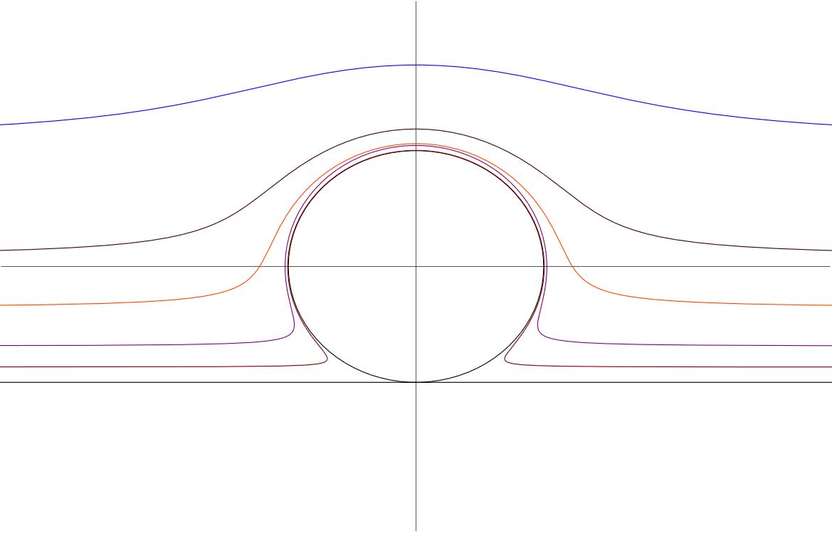
Figure 1. A family of Conchoids of de Sluze

Remark 4.2.

In a similar manner we can fix the nodes and the coefficients of the quadrature identity and construct a rational conformal mapping of the form (2.4) –(2.5). This will result in a system of algebraic equations that has one free parameter, and hence provides examples of families of domains such that each one of them is a QD of the same distribution.

Example 4.3.

Following Strakhov’s example we construct a family of QDs where a parabola is the asymptote of the boundary. We consider a map

(4.3) $$z=\psi(w)=2w+iw^{2}+ih+\frac{a}{w-ib},\quad w\in\mathbb{H}_{-},\ a,b>0,\ h\in{\mathord{\mathbb{R}}}.$$

Assuming for a moment that the map $\psi$ is univalent, and requiring that $\psi(-ib)=0$ and that the Schwarz function has residue one at the origin, then we get the following two equations

(4.4) $$\left\{\begin{array}[]{l}h=2b+b^{2}-\frac{a}{2b}\\ 2a+2ab+\frac{a^{2}}{4b^{2}}=1\end{array}\right..$$

Since the algebraic equations (4.4) has one parameter free, there is a family of conformal mappings $\psi_{a}$ such that $\Omega_{a}=\psi_{a}(\mathbb{H}_{-})$ is a QD of the unit Dirac measure. Our aim is to let $a,b$ tend to zero in a such manner that $\Omega_{a}$ will converge. From the second equation of (4.4) we see that the condition

(4.5) $$\lim_{a,b\to 0}\frac{a}{b}=2$$

is demanded.

In order to assure that the map $\psi_{a}$ is univalent, we will show that for an appropriate choice of small parameters $a$ and $b$ it maps the real line onto a curve without closed loops. To see this we let $z(t)=X(t)+iY(t)$, where

(4.6) $$X(t)=2t+\frac{at}{t^{2}+b^{2}},\qquad Y(t)=t^{2}+h+\frac{ab}{t^{2}+b^{2}},$$

be the parametric presentation of the boundary of $\Omega_{a}$, and we shall and analyze the critical points of these functions. Furthermore, since $X$ is an odd function and $Y$ is an even, it suffices to examine the critical points only for positive $t$. Computing the derivatives

(4.7) $$\frac{dX}{dt}(t)=\frac{2(t^{2}+b^{2})^{2}+a(b^{2}-t^{2})}{(t^{2}+b^{2})^{2}},\qquad\frac{dY}{dt}(t)=2t-\frac{2abt}{(t^{2}+b^{2})^{2}},$$

we find that the function $Y$ has critical points when $t^{2}=b\sqrt{\frac{a}{b}}-b^{2}$ and $b\sqrt{\frac{a}{b}}-b^{2}\geq 0$. The critical points of $X$ satisfy the equation $t^{2}=\frac{1}{4}\left(\pm\sqrt{a^{2}-16ab^{2}}+a-4b^{2}\right)$. This equation has two positive roots when $a$ and $b$ are small. Now, the contour $z(t)=X(t)+iY(t)$ will have a closed loop for positive $t$ if and only if the critical point of $Y$ is in between the two critical points of $X$. The largest root is approximately $\frac{1}{4}\left(2a-12b^{2}\right)$ , and since by (4.7) $a\simeq 2b$, it is less than $b\sqrt{\frac{a}{b}}-b^{2}$ for small $b$. So we conclude that the curve $z(t)$ has no closed loops when $a$ and $b$ are sufficiently small.

Having showed that $\psi_{a}$ is univalent, we turn now to compute the limit of the boundary of $\Omega_{a}$, $\Gamma_{a}=\psi_{a}({\mathord{\mathbb{R}}})$, as $a$ and $b$ tend to zero. However, unlike Example 4.1, we do not know the explicit representation of the boundary. Therefore we make the variable change

$$\cos\theta=\frac{1}{\sqrt{(t/b)^{2}+1}},\qquad\sin\theta=\frac{t/b}{\sqrt{(t/b)^{2}+1}},\quad-\frac{\pi}{2}<\theta<\frac{\pi}{2}.$$

Then (4.6) becomes

(4.8) $$X(\theta)=2b\tan\theta+\frac{a}{b}\sin\theta\cos\theta,\qquad Y(\theta)=b^{2}\tan^{2}\theta+h+\frac{a}{b}\cos^{2}\theta.$$

By (4.4) and (4.5), $\lim_{a,b\to 0}h=-1$. Therefore, for any $\epsilon>0$ and $\theta\in[-\frac{\pi}{2}+\epsilon,\frac{\pi}{2}-\epsilon]$, the curve (4.8) tends to

$$X(\theta)=2\sin\theta\cos\theta=\sin 2\theta,\qquad Y(\theta)=2\cos^{2}\theta-1=\cos 2\theta.$$

On the other hand, we see that for $t^{2}\geq b$

$$|X(t)-2t|=\frac{a|t|}{t^{2}+b^{2}}=\frac{a}{|t|}\frac{1}{1+\left(\frac{b}{t}\right)^{2}}\leq\left(\frac{a}{b}\right)\sqrt{b}\to 0$$

and

$$|Y(t)-(t^{2}-1)|\leq|h+1|+\frac{a}{1+b}\to 0,$$

as $(a,b)\to(0,0)$ and equations (4.4) hold. Thus the family of curves $\Gamma_{a}$ tends to a union of the unit circle and the parabola $y+1=(x/2)^{2}$. The family of simply connected QDs converges to $B_{1}(0)\cup\left\{y<\left({x}/{2}\right)^{2}-1\right\},$ that is, a union of null QD and a disk.

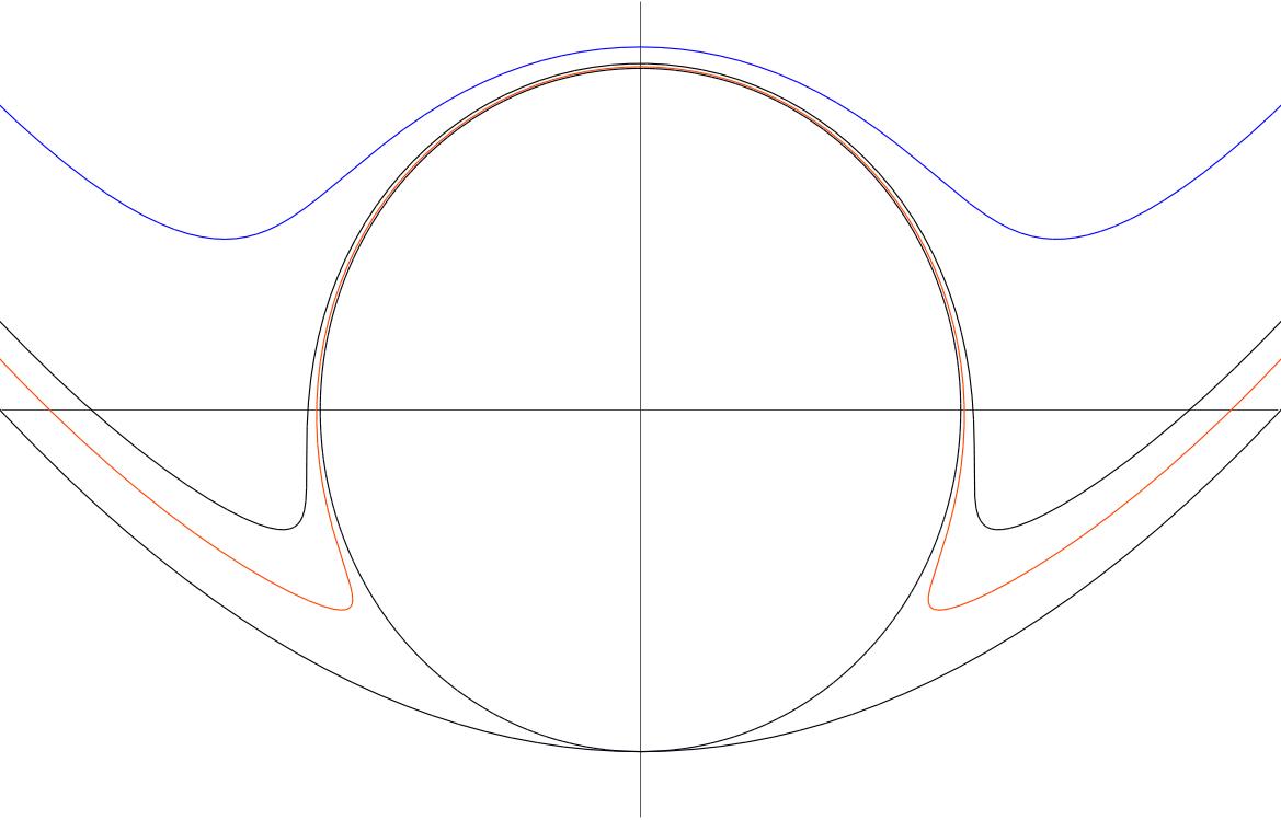
Figure 2. A family converging to a parabola and a circle

The existence of a QD for a positive measure and with an infinite ray as an asymptote of the boundary is not evident. It cannot be constructed by Sakai’s variational method [17, Ch. 11], since this method requires that the complement of the attached null QD has non–empty interior. Nevertheless, by using similar ideas as in examples 4.1 and 4.3 we are able to construct a family of QDs for a positive Dirac measure at zero and with the positive $x$–axis as the asymptote of the boundary. In contrast with the previous two examples, the boundary of the family cannot converge to a union of a circle and a ray, since this contradicts the regularity of the Schwarz function [18].

Example 4.4.

We consider a conformal map

(4.9) $$z=\psi(w)=w^{2}+h-\frac{ia}{w-ib},\quad b>0,\ a,h\in{\mathord{\mathbb{R}}}$$

from $\mathbb{H}_{-}$ to the domain $\Omega$. Then the requirements that $\psi(-ib)=0$, the Schwarz function has residue one at $z=0$, and the origin belongs to the image of $\psi$, leads to the following relations:

(4.10a) $$h=b^{2}-\frac{a}{2b}$$

(4.10b) $$8b^{3}a-4b^{2}+a^{2}=0$$

(4.10c) $$h+\frac{a}{b}=b^{2}+\frac{a}{2b}>0.$$

For $a<0$ relations (4.10) cannot hold. When $a>0$, we find by computing the minimum of the third degree polynomial in (4.10b) that it has positive roots only when $a\leq\sqrt[4]{4/27}$. For that range of $a$ there are two types of QDs.

For both types we need to check that the map (4.9) is conformal. We do this by checking the conditions which guarantee that the real line is mapped in a one to one manner onto the curve

(4.11) $$X(t)=t^{2}+h+\frac{ab}{t^{2}+b^{2}},\qquad Y(t)=\frac{-at}{t^{2}+b^{2}},\ t\in{\mathord{\mathbb{R}}}.$$

The first type is when the function $X$ has critical points for $t\neq 0$, this occurs when $t^{2}=\sqrt{ab}-b^{2}$, which implies that $b^{3}<a$. Then the curve (4.11) will not have a closed loop if the critical points of $Y$ appear “after” the critical points of $X$, which means that $b^{2}\geq\sqrt{ab}-b^{2}$. Thus in that case we have to require that the largest root of (4.10b) will satisfy the condition $b^{3}<a<4b^{3}$.

The second type is where the function $X$ is monotone for $t\gtrless 0$. Also, in that case that the largest root of (4.10b) needs to satisfy the condition $b^{3}>a$. Note that if $a<1/3$, then the largest root is greater than one and hence this condition is satisfied.

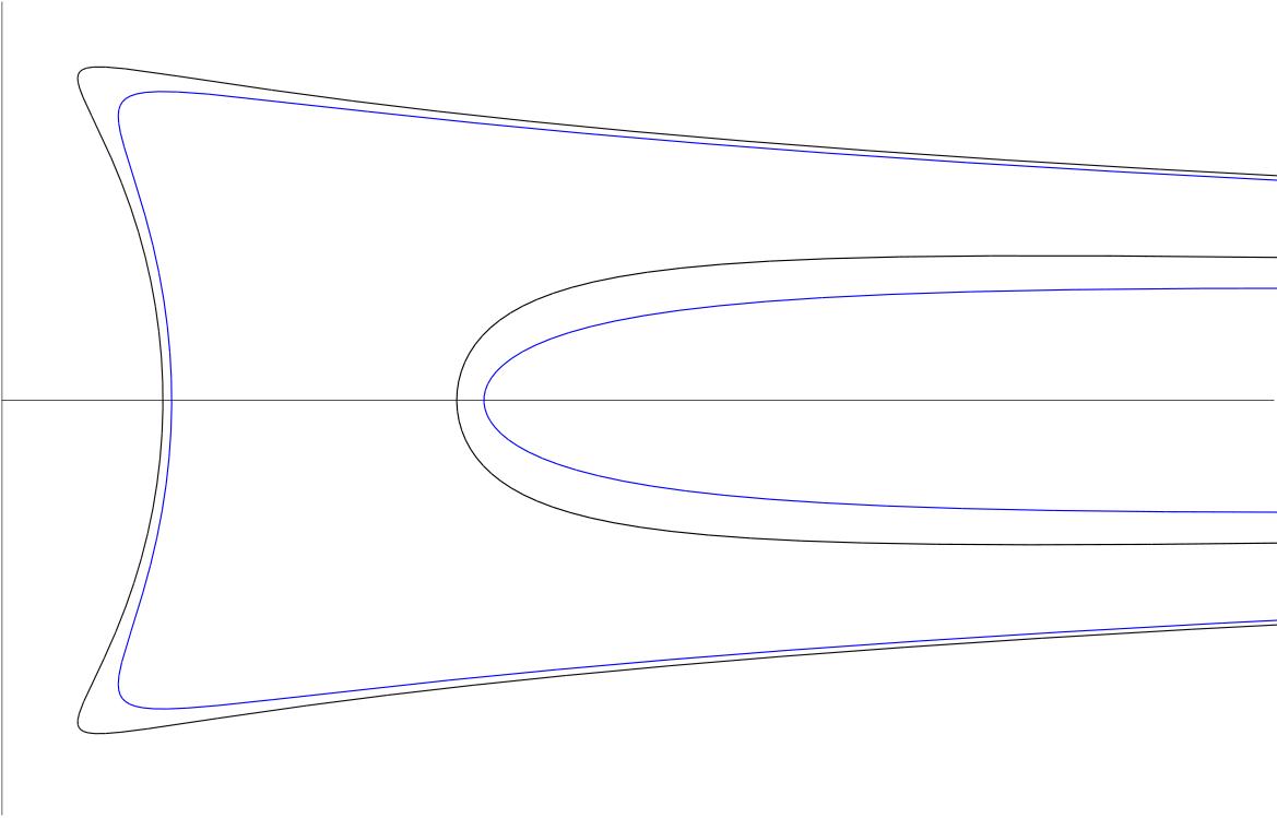
Figure 3. Two types of QDs for the Dirac measure and a ray as an asymptote

5. Summary

By means of conformal mappings we established the asymptotic behavior of the boundary of unbounded quadrature domains in the plane and when the infinity point belongs to the boundary. Although this tool is not available in higher dimensions, we hope the present paper will stimulate further investigations of unbounded quadrature domains in the space. The specific form of the conformal mapping from the lower half plane enables the construction of families of quadrature domains of the Dirac measure at a given point and possessing a given type of the asymptote.

Acknowledgement. I would like to thanks Avmir Margulis for many valuable talks and enlightening comments. I also grateful to the anonymous referee for his/her constructive comments, which definitely contributed to the improvement of the manuscript.

References

• [1] D. Aharonov and H.S. Shapiro, Domains on which analytic functions satisfy quadrature identities, J. Analyse Math. 30 (1976), 39–73.
• [2] L. Bers, An approximation theorem, J. Analyse Math. 14 (1965), 1–4.
• [3] P. Davis, The Schwarz Function and Its Application, Carus Mathematical Monographs, vol. 14, The Mathematical Association of America, 1974.
• [4] N.V. Fedorova and A.V. Tsirulskiy, The solvability in finite form of the inverse logarithmic potential problem for contact surface, Physics of the Solid Earth 12 (1976), 660–665, (translated from Russian).
• [5] S. J. Gardiner and T. Sjödin, Convexity and the exterior inverse problem of potential theory, Proc. Amer. Math. Soc. 136 (2008), no. 5, 1699–1703.
• [6] B. Gustafsson, Quadrature identities and the schottky double, Acta Appl. Math. 1 (1983), 209–240.
• [7] by same author, On quadrature domains and on an inverse problem in potential theory, J. Analyse Math 44 (1990), 172–215.
• [8] W.K. Hayman, L. Karp, and H.S. Shapiro, Newtonian capacity and quasi balayage, Rend. Mat. Appl. 20 (2000), no. 7, 93–129.
• [9] V. Isakov, Inverse Source Problems, Surveys and Monographs, vol. 34, Amer. Math. Soc., Providence, RI, 1993.
• [10] V.K. Ivanov, On the solvability of the inverse problem of the logarithmic potential in finite terms, Doklady of SSSR Acad. Sci, Mathematics 104 (1956), no. 4, 598–599, (in Russian).
• [11] L. Karp and A.S. Margulis, Newtonian potential theory for unbounded sources and applications to free boundary problems, J. Analyse Math. 70 (1996), 1–63.
• [12] L. Karp and H. Shahgholian, Regularity of a free boundary problem near the infinity point, Comm. Partial Differential Equations 25 (2000), no. 11-12, 2055–2086.
• [13] S.Y. Lee and N.G. Makarov, Topology of quadrature domains, arXiv.org (2013).
• [14] A.S. Margulis, The moving boundary problem of potential theory, Adv. Math. Sci. Appl. 5 (1995), no. 2, 603–629.
• [15] P.S. Novikov, On the inverse problem of potential, Dokl. Akad. Nauk SSSR 18 (1938), 165–168, (translated from Russian).
• [16] M. Sakai, Null quadrature domains, J. Analyse Math. 40 (1981), 144–154.
• [17] by same author, Quadrature Domains, Lecture Notes in Mathematics, vol. 934, Springer-Verlag, Berlin-Heidelberg-New York, 1982.
• [18] by same author, Regularity of a boundary having a schwarz function, Acta Math. 166 (1991), 263–297.
• [19] by same author, Regularity of boundaries of quadrature domains in two dimensions, SIAM J. Math. Anal. 24 (1993), 341–364.
• [20] by same author, Quadrature domains with infinite volume, Complex Analysis and Operator Theory 3 (2009), no. 2, 525–549.
• [21] H. S. Shapiro, The Schwarz Function and Its Generalization to Higher Dimensions, Arkansas Lecture Notes in the Mathematical Sciences, vol. 9, John Wily & Sons, Inc., New York, 1992.
• [22] H.S. Shapiro, Unbounded quadrature domains, Complex Analysis I (C. Berenstein, ed.), Lecture Notes in Mathematics, vol. 1275, Springer-Verlag, 1987, pp. 287–331.
• [23] V.N. Strakhov, The inverse logarithmic potential problem for contact surface, Physics of the Solid Earth 10 (1974), 104–114, (translated from Russian).
• [24] by same author, The inverse problem of the logarithmic potential for contact surface, Physics of the Solid Earth 10 (1974), 369–379, (translated from Russian).
• [25] A.V. Tsirulskiy, Some properties of the complex logarithmic potential of a homogeneous region, Bull. (Izv.) Acad. Sci. USSR Geophys. Ser. (1963), 653–655, (Russian).
• [26] L. Zalcman, Some inverse problems of potential theory, Integral Geometry (Providence, RI), Contemp. Math., vol. 63, Amer. Math. Soc., 1987, pp. 337–350.