Critical Casimir Forces for Films with Bulk Ordering Fields

Abstract

The confinement of long-ranged critical fluctuations in the vicinity of second-order phase transitions in fluids generates critical Casimir forces acting on confining surfaces or among particles immersed in a critical solvent. This is realized in binary liquid mixtures close to their consolute point $T_{c}$ which belong to the universality class of the Ising model. The deviation of the difference of the chemical potentials of the two species of the mixture from its value at criticality corresponds to the bulk magnetic filed of the Ising model. By using Monte Carlo simulations for this latter representative of the corresponding universality class we compute the critical Casimir force as a function of the bulk ordering field at the critical temperature $T=T_{c}$. We use a coupling parameter scheme for the computation of the underlying free energy differences and an energy-magnetization integration method for computing the bulk free energy density which is a necessary ingredient. By taking into account finite-size corrections, for various types of boundary conditions we determine the universal Casimir force scaling function as a function of the scaling variable associated with the bulk field. Our numerical data are compared with analytic results obtained from mean-field theory.

In the vicinity of second-order phase transitions long-ranged fluctuations of the corresponding order parameter arise. Fisher and de Gennes pointed out that in fluids the spatial confinement of such fluctuations produces effective forces acting on the confining surfaces FdG . In view of certain similarities with the electromagnetic Casimir effect Casimir ; KG , in which such forces are induced by the quantum fluctuations of the electromagnetic field, these forces in critically fluctuating media are called critical Casimir forces (CCF) Krech ; BDT ; Gambassi . In line with the finite size scaling concept Barber ; Privman CCF are characterized by universal scaling functions depending on the ratio of the distance between the confining surfaces and the bulk correlation length $\xi$, which diverges upon approaching the critical point $T_{c}$ Krech ; BDT ; Gambassi . The scaling function depends on the bulk universality class and on the type of boundary conditions (BC) for the order parameter. For classical binary liquids mixtures, which belong to the Ising bulk universality class, CCF have been measured experimentally both indirectly via their influence on wetting films Fukuto and directly by monitoring a colloidal particle near a wall and immersed in a critical solvent nature ; PRE1 . There is excellent agreement between these experimental data and the corresponding theoretical results EPL ; PRE ; sp .

Figure 1(a) shows the schematic bulk phase diagram for the type of binary liquid mixtures (such as water-lutidine) used in these experiments Fukuto ; nature ; PRE1 ; they exhibit a lower critical point $(T_{c},c_{A}^{c})$ where $c_{A}$ denotes the concentration of one of the two components $A$ and $B$ (e.g., lutidine) of the mixture. Long-ranged fluctuations of the order parameter $\psi\sim c_{A}-c_{A}^{c}$ arise upon approaching this point either along an iso-concentration $c_{A}=c_{A}^{c}$ path or along an isotherm $T=T_{c}$ (or any other direction). The phase diagram for the corresponding Ising model is shown in Fig. 1(b). The bulk magnetic field $H$ plays the role of $\mu_{A}-\mu_{B}-(\mu_{A}-\mu_{B})_{c}$ where $\mu_{A,B}$ are the chemical potentials of the two species of the fluid. Together with the reduced temperature $t=(T-T_{c})/T_{c}$ this difference determines the order parameter $c_{A}-c_{A}^{c}$. The scaling functions of CCF depend strongly on the BC. Generically, one of the two species of the binary mixture is preferentially adsorbed at a confining wall which within the Ising model corresponds to the presence of a (strong) surface field, denoted as $(+)$ or $(-)$ BC. If the surface is neutral with respect to the two species one is lead to Dirichlet BC (denoted as (O) ) Diehl . For the Ising universality class and in the presence of surface fields the variation of the CCF upon varying the BC has been studied experimentally Nellen , theoretically Mohry , and numerically Hass ; Surf . One finds a continuous crossover between attractive CCF for $(+,+)$ BC and repulsive ones for $(+,-)$ BC. There is experimental evidence that CCF do not only depend sensitively on temperature but also on $c_{A}$ BE ; Nellen1 . However, whereas there is by now rather reliable theoretical knowledge concerning the temperature dependence of CCF EPL ; PRE ; Hass ; Surf , there are only a few studies of their concentration dependence; they are either pure mean-field studies SHD or scaling-theory enhanced mean-field studies Mohry1 ; BCPP1 ; BCPP2 . For spatial dimension $d=2$ the CCF in the presence of a bulk magnetic field have been studied in detail in Refs. DMC ; MDC ; MDE .

In particular, for spatial dimension $d=3$ there are no simulation data available concerning the dependence of the CCF on the bulk magnetic field within the Ising universality class. The present study closes this gap and provides insight into the scaling behavior of CCF in the full neighborhood of the critical point for four sets of BC: $(+,+)$, $(-,+)$, $(O,+)$, and $(O,O)$.

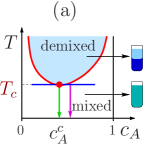
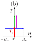
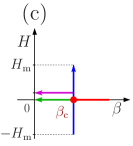
Figure 1: (a) Schematic phase diagram of demixing in binary liquid mixtures with a lower critical point at $(T=T_{c},c_{A}=c_{A}^{c})$ where $T$ is the temperature and $c_{A}$ is the concentration of one of the two species of the mixture. The green, magenta, and blue full lines indicate three distinct thermodynamic paths. (b) Phase diagram of the Ising model in the $(H,T)$ plane where $H$ is the bulk field. Note that two-phase coexistence for $T\geq T_{c}$ in (a) corresponds to $(H=0,T\leq T_{c})$ in (b). The isotherm runs in the interval $|H|\leq H_{\mathrm{m}}$ (see main text) and the magenta path corresponds to $(T>T_{c},H=0.17H_{\mathrm{m}})$. (c) Phase diagram and corresponding paths in the $(\beta=1/(k_{\mathrm{B}}T),H)$ plane with $\beta_{c}=1/(k_{\mathrm{B}}T_{c})$.

We consider a simple cubic lattice with lattice spacing $a$. (On the lattice all lengths are measured in units of $a$ and thus are dimensionless.) The lattice sites form a slab $L_{x}\times L_{y}\times L_{z}$ with $L_{x}=L_{y}=6L_{z}$ and with a cross-section $A=L_{x}\times L_{y}$. There are periodic BC along the $x$ and $y$ axes. In our study we have carried out simulations for $L_{z}=10,15$, and 20.

Each lattice site $i=(1\leq x\leq L_{x},1\leq y\leq L_{y},1\leq z\leq L_{z})$ is occupied by a spin $s_{i}=\pm 1$. The Hamiltonian of the Ising model with bulk ($H$) and surface fields ($H_{1}^{\pm}$, acting on the bottom [$-$] and the top [$+$] layers $z=1,L_{z}$, respectively) is

$${\cal H}=-\sum_{\langle{\rm ij}\rangle}s_{i}s_{j}-H\sum_{k}s_{k}-H_{1}^{-}\sum_{\langle\mathrm{bot.}\rangle}s_{j}-H_{1}^{+}\sum_{\langle\mathrm{top}\rangle}s_{j}.$$ (1)

Here and in the following the energies and fields are measured in units of the spin-spin interaction constant $J$. The sum $\langle{\rm ij}\rangle$ is taken over all nearest-neighbor pairs of sites on the lattice and the sum over $k$ runs over all spins. The four types of BC which we study correspond to $(H_{1}^{-},H_{1}^{+})=(+\infty,+\infty)\equiv(+,+)$, $(-\infty,+\infty)\equiv(-,+)$, $(0,+\infty)\equiv(O,+)$, and $(0,0)\equiv(O,O)$. In practice, we use surface fields which are finite but strong enough to observe saturation of results and thus mimic the action of infinite surface fields Surf . Finite surface fields give rise to a dependence on the scaling variables $H_{1}^{\pm}L_{z}^{\Delta_{1}/\nu}$ Diehl ; we use $H_{1}L_{z}^{\Delta_{1}/\nu}=+100$ and $H_{1}L_{z}^{\Delta_{1}/\nu}=-100$ instead of $+\infty$ and $-\infty$, respectively. Here $\nu=0.6301(4)$ PV is the critical exponent of the bulk correlation length $\xi^{\pm}_{t}\left(t=\frac{T-T_{c_{\mbox{\rule{0.0pt}{2.5pt}}}}}{T_{c}}\to\pm 0,H=0\right)=\xi_{t,0}^{\pm}|t|^{-\nu}$, and $\Delta_{1}=0.46(2)$ GZ is the so-called critical surface gap exponent. For these large values for $H_{1}^{\pm}$ and $A$ the system depends de facto only on the three parameters $\beta=1/(k_{\mathrm{B}}T)$, $H$, and $L_{z}$. The critical value of $\beta$ is $\beta_{c}=1/(k_{B}T_{c})=0.2216544(3)$ RZW .

According to finite-size scaling theory fisher_nakanishi , for given BC and number of layers $L_{z}$ the thermodynamic state of the system is characterized by two scaling variables: $(L_{z}/\xi_{t},HL_{z}^{\Delta/\nu})$, where $HL_{z}^{\Delta/\nu}$ is the bulk magnetic field scaling variable with $\Delta=1.5637(14)$ PV .

For large values of $A$, the total free energy $F(\beta,H,L_{z})$ of the film can be written as $F(\beta,H,L_{z})=A\beta^{-1}[L_{z}f^{\mathrm{b}}(\beta,H)+f^{\mathrm{ex}}(\beta,H,L_{z})]$. Here $f^{\mathrm{b}}(\beta,H)$ is the bulk free energy density per $k_{\mathrm{B}}T$ of the macroscopic system at a given temperature and bulk magnetic field. The excess free energy $f^{\mathrm{ex}}$ per area gives rise to the critical Casimir force $f_{\mathrm{C}}$ in units of $k_{\mathrm{B}}T$ and $A$: $f_{\mathrm{C}}(\beta,H,L_{z})\equiv-\partial f^{\mathrm{ex}}(\beta,H,L_{z})/\partial L_{z}$. For given BC, on a lattice (we denote lattice quantities by symbols with a “hat” $\,\hat{}\,$ ) we replace the derivative by the finite difference

$$\hat{f}_{\mathrm{C}}^{(BC)}\left(\beta,H,L\right):=-\frac{\beta\Delta\hat{F}^{(BC)}(\beta,H,L_{z},A)}{A}+\hat{f}^{\mathrm{b}}(\beta,H)\,,$$ (2)

where $\Delta\hat{F}^{(BC)}(\beta,H,L_{z},A)=\hat{F}^{(BC)}(\beta,H,L_{z},A)-\hat{F}^{(BC)}(\beta,H,L_{z}-1,A)$. Here we express the CCF in terms of the film thickness $L:=L_{z}-\frac{1}{2}$ which is a half-integer quantity.

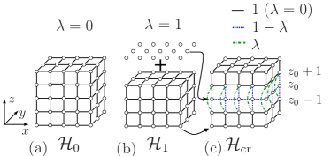
Figure 2: Arrangement of bonds for determining the free energy difference between systems with Hamiltonian ${\cal H}_{0}$ and $L_{z}$ layers (a) and with Hamiltonian ${\cal H}_{1}$ and $L_{z}-1$ layers plus $A=L_{x}\times L_{y}$ isolated spins (b). The crossover Hamiltonian ${\cal H}_{\rm cr}={\cal H}_{0}+\lambda({\cal H}_{1}-{\cal H}_{0})$ interpolates between ${\cal H}_{0}$ and ${\cal H}_{1}$ upon changing $\lambda$ from 0 to 1 (c).

In accordance with eq. (2), we determine the film free energy difference $\Delta\hat{F}^{(BC)}$ and the bulk free energy $\hat{f}^{\mathrm{b}}$ per spin and per $k_{\mathrm{B}}T$ as functions of the bulk magnetic field $H$ at $T_{c}$. To this end we use the coupling parameter approach (see Refs. Mon ; PRE ; Surf ). In this context ${\cal H}_{0}$ denotes the Hamiltonian of the system with $L_{z}$ layers [Fig. 2(a)] and ${\cal H}_{1}$ is the Hamiltonian of the system with $L_{z}-1$ layers plus a layer of $A=L_{x}\times L_{y}$ isolated spins [Fig. 2(b)] which keeps the number of spins in the system constant. We introduce the crossover Hamiltonian ${\cal H}_{\rm cr}(\lambda)={\cal H}_{0}+\lambda\Delta{\cal H}$, with $\Delta{\cal H}={\cal H}_{1}-{\cal H}_{0}$, which interpolates between ${\cal H}_{0}$ and ${\cal H}_{1}$, upon changing the coupling parameter $\lambda$ from 0 to 1, by suitably varying certain interaction constants as $\lambda$ and $1-\lambda$ (see Fig. 2(c)) for a selected layer at height $z_{0}=L_{z}/2\;[(L_{z}+1)/2]$ for even [odd] values of $L_{z}$. The free energy difference between these two systems is $\Delta F=\int_{0}^{1}F^{\prime}_{\rm cr}(\lambda){\rm d}\lambda=\int_{0}^{1}\langle\Delta{\cal H}\rangle_{\rm cr}(\lambda){\rm d}\lambda$ where the free energy $F_{\rm cr}(\lambda)$ corresponds to ${\cal H}_{\rm cr}(\lambda)$ and its derivative $F^{\prime}_{\rm cr}(\lambda)=\frac{\mathrm{d}}{{\mathrm{d}}\lambda}F(\lambda)=\langle\Delta{\cal H}\rangle_{\rm cr}(\lambda)$ takes the form of the canonical ensemble average $\langle\ldots\rangle_{\rm cr}(\lambda)$ taken with $\exp(-\beta{\cal H_{\rm cr}})$ of the energy difference $\Delta{\cal H}$. We have determined the ensemble averages $\langle\Delta{\cal H}\rangle_{\rm cr}(\lambda)$ via MC simulations for $N_{\lambda}=21$ different values of $\lambda_{k}=\frac{k}{N_{\lambda}-1}$ ($k=0,\dots,N_{\lambda}-1$) by using the hybrid MC method with a mixture of Wolff and Metropolis algorithms. For the computation of the thermal average we have used $5\times 10^{5}$ MC steps [$10^{6}$ for $(O,O)$ BC]. Based on $N_{\lambda}$ points we have performed the numerical integration over $\lambda$ by using Simpson’s rule. Accordingly, the free energy difference appearing in eq. (2) is given by

$$\Delta\hat{F}^{(BC)}(\beta,H,L,A)=$$ (3)

$$-\int_{0}^{1}\langle\Delta{\cal H}\rangle_{\rm cr}(\lambda){\rm d}\lambda-A\beta^{-1}\ln[2\cosh(\beta H)],$$

where the last term corresponds to the free energy of $A$ isolated spins.

Once $\Delta\hat{F}^{(BC)}(\beta,H,L,A)$ has been computed, one still has to separate off $\hat{f}^{\mathrm{b}}(\beta_{c},H)$ from it [see eq. (2)] in order to obtain the Casimir force. In the absence of the bulk magnetic field $H$ the bulk free energy can be determined via temperature integration hucht ; hasen1 ; hasen2 . We extend this method to the case $H\neq 0$. To this end, as in Ref. Surf , we determine the free energy density for a cube of volume $L_{\rm cube}^{3}=128^{3}$ with periodic BC in all directions. We consider this value as the desired bulk free energy density (per $k_{\mathrm{B}}T$): $\hat{f}^{\mathrm{b}}(\beta,H)\simeq\hat{f}^{\mathrm{cube}}(\beta,H,L_{\mathrm{cube}}=128)$. In order to obtain $\hat{f}^{\rm cube}$ we have integrated the appropriate combination $E(\beta^{\prime},H)-HM(\beta^{\prime},H)$ of the energy and the magnetization:

$$\hat{f}^{\mathrm{cube}}(\beta,H)=-\ln(2)+$$ (4)

$$L_{\rm cube}^{-3}\int\limits_{0}^{\beta}\left[E(\beta^{\prime},H)-HM(\beta^{\prime},H)\right]{\rm d}\beta^{\prime},$$

where $E(\beta,H)=-\langle\sum\limits_{\langle i,j\rangle}s_{i}s_{j}\rangle_{\mathcal{H}(H)}$ and $M(\beta,H)=\langle\sum\limits_{k}s_{k}\rangle_{\mathcal{H}(H)}$ are the energy and the magnetization, respectively, of a system at an inverse temperature $\beta$ and with a bulk magnetic field $H$.

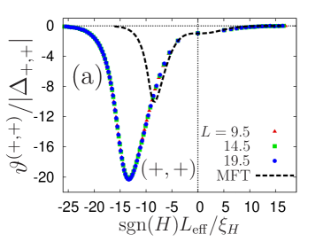
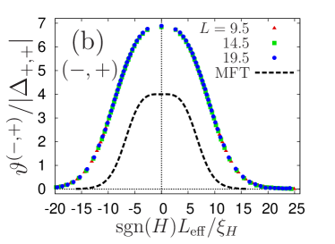
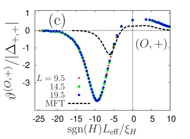
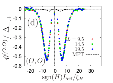
Figure 3: The MC data points show the universal scaling functions (eq. (7)) $\vartheta^{(BC)}/|\Delta_{++}|$ for $d=3$, $T=T_{c}$, and $L=L_{\mathrm{eff}}-\delta L=9.5,14.5$, and $19.5$ (Table 1) normalized by the critical Casimir amplitude $\Delta_{++}(d=3)\simeq-0.75(6)$ ($T=T_{c}$ and $H=0$) PRE , as functions of the scaling variable ${\mathrm{sgn}}(H)L_{\mathrm{eff}}/\xi_{H}$ for four BC: (a) $(+,+)$; (b) $(-,+)$; (c) $(O,+)$; (d) $(O,O)$. The dashed lines show the corresponding normalized (by $\tilde{\Delta}_{++}(d=4)$) universal scaling functions in $d=4$, as obtained within MFT and as function of ${\mathrm{sgn}}(\tilde{H})\tilde{L}/\xi_{\tilde{H}}$. The MFT expressions for $\tilde{\vartheta}$ carry, inter alia, an undetermined prefactor $g^{-1/2}$. This dependence on $g$ drops out upon choosing the above normalization, rendering a universal ratio in $d=4$. Accordingly, in (a) both the MC data and the MFT results attain the value 1 at the origin and in (b) the MFT result attains the value 4 there. In (d) the MFT result has a zero at the origin whereas the MC data are slightly nonzero there. The results in (b) and (d) are symmetric around the origin. Note the different scales of the axes.

${\cal H}(H)$ is given by eq. (1) with $H_{1}^{\pm}=0$. Knowing the free energy density $\hat{f}^{\mathrm{b}}(\beta,H_{0})$ at a certain value $H_{0}$ of the bulk magnetic field one can compute the bulk free energy density for an arbitrary value of the magnetic field $H$ via integration:

$$\hat{f}^{\mathrm{b}}(\beta,H)=\hat{f}^{\mathrm{b}}(\beta,H_{0})-\beta L_{\rm cube}^{-3}\int\limits_{H_{0}}^{H}M(\beta,H^{\prime}){\rm d}H^{\prime}.$$ (5)

By using eqs. (4) and (5) we have performed numerical integrations along the three paths shown in Fig. 1(c): $(\beta,H=0)$ [green], $(\beta,H=0.1)$ [magenta], and $(\beta=\beta_{c},H)~{}$[blue]. We have employed a histogram reweighting method FS ; LB for improving the accuracy of the numerical integration. Accordingly, for 165 points of $\beta$ in the interval $[0,\beta_{c}]$ we have computed histograms (averaged over $10^{6}$ MC steps) of the quantities $E(\beta,H=0)$ and $E(\beta,H=0.1)-0.1M(\beta,H=0.1)$. We have also computed the histogram of $M(\beta_{c},H)$ for 256 points of the bulk field $H$ in the interval $0\leq H\leq H_{\mathrm{m}}$ where $H_{\mathrm{m}}=0.59$ (see Figs. 1(b) and (c)). For negative values of $H$ we have used the symmetry relation $f^{\mathrm{b}}(\beta,-H)=f^{\mathrm{b}}(\beta,H)$. In a second step we have performed numerical integration along these trajectories using histogram reweighting with the trapezoid rule using $10^{5}$ points. Integrating along the green line $(\beta,H=0)$ we have obtained the critical value $\hat{f}^{\mathrm{b}}(\beta_{c},H=0)=-0.77785038(36)$ whereas sequentially integrating along the magenta $(\beta,H=0.1)$ and blue $(\beta_{c},H)$ line, we have obtained the value $\hat{f}^{\mathrm{b}}(\beta_{c},H=0)=-0.77784921(60)$ which de facto coincides within the numerical accuracy with the former value. To the best of our knowledge, the dependence of the bulk free energy $\hat{f}_{\mathrm{b}}$ of the $d=3$ Ising model as a function of the bulk magnetic field $H$ is not yet available and the present analysis closes this gap. Finally, we combine the results for the bulk free energy $\hat{f}^{\mathrm{b}}(\beta_{c},H)$ with the corresponding ones for the free energy difference $\Delta\hat{F}^{(BC)}(\beta,H,L,A)$ leading to the critical Casimir force

$$\hat{f}_{\mathrm{C}}^{(BC)}(\beta_{c},H,L)=\beta_{c}A^{-1}\int_{0}^{1}\langle\Delta{\cal H}\rangle_{\rm cr}(\lambda){\rm d}\lambda$$ (6)

$$+\hat{f}^{\mathrm{b}}(\beta_{c},H)+\ln[2\cosh(\beta_{c}H)].$$

The numerical accuracy of $\hat{f}_{\mathrm{C}}^{(BC)}$ is determined in a standard way by subdividing the numerical results into 10 series.

On the basis of finite-size scaling theory Barber ; nature ; PRE1 ; EPL ; PRE ; sp ; Diehl , in spatial dimension $d$ CCF in units of $k_{\mathrm{B}}T$ and per $d-1$-dimensional area are expected to exhibit the scaling form

$$\hat{f}_{\mathrm{C}}^{(BC)}(\beta,H,L)=L_{\mathrm{eff}}^{-d}\vartheta^{(BC)}_{\pm}\left(L_{\mathrm{eff}}/\xi_{t}^{\pm},L_{\mathrm{eff}}/\xi_{H}\right),$$ (7)

where the universal scaling function $\vartheta^{(BC)}_{\pm}$ depends on the boundary conditions at the top and at the bottom surface, and $\xi_{H}=\xi_{H,0}|H|^{-\nu/\Delta}$ is the bulk correlation length at $T=T_{c}$. (Concerning the relationship between the scaling variable $h=HL_{\mathrm{eff}}^{\Delta/\nu}\sim\left(L_{\mathrm{eff}}/\xi_{H}\right)^{\Delta/\nu}$ and the physical quantity $(c_{A}-c_{A}^{c})/c_{A}^{c}$ see Subsec. II.B.1 in Ref. PRE1 , Subsec. II.B.2 and the Appendix in Ref. Mohry1 , and Ref. SHD .) In eq. (7), for each BC we use an effective thickness $L_{\mathrm{eff}}=L+\delta L$ such that, to a certain extent, $\delta L$ captures some corrections to scaling Surf ; Hass . Since here we are studying the behavior of the CCF at the critical temperature $\beta_{c}$, one has $L_{\mathrm{eff}}/\xi_{t}^{\pm}=0$; thus in the following we omit the first argument of $\vartheta_{\pm}^{(BC)}(0,L_{\mathrm{eff}}/\xi_{H})\equiv\vartheta^{(BC)}(L_{\mathrm{eff}}/\xi_{H})$. We apply the fitting procedure described in the Appendix of Ref. PRE which for each type of BC minimizes the spread among the results for $\vartheta^{(BC)}$ as obtained for various values of $L\;(=9.5,14.5,19.5)$. This procedure renders the correction $\delta L$ to scaling (see Table 1).

Table 1: Correction $\delta L$ to scaling for four BC.

(BC)	$(+,+)$	$(-,+)$	$(O,+)$	$(O,O)$
$\delta L$	0.60(10)	0.65(2)	0.93(10)	1.22(2)

In Figs. 3 and 4 we plot the results for the CCF scaling function $\vartheta^{(BC)}$ as a function of the scaling variable $\mathrm{sgn}(H)L_{\mathrm{eff}}/\xi_{H}$ for the BC $(+,+)$, $(-,+)$, $(O,+)$, and $(O,O)$, respectively. Along the critical isotherm one has $\xi_{H}=\xi_{H,0}|H|^{-\nu/\Delta}$ where $\xi_{H,0}=0.3048(9)$ (see Ref. EFS ). After taking into account the aforementioned finite size corrections $\delta L^{(BC)}$, for each BC we observe data collapse onto a master curve for different values of $L$.

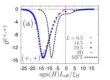
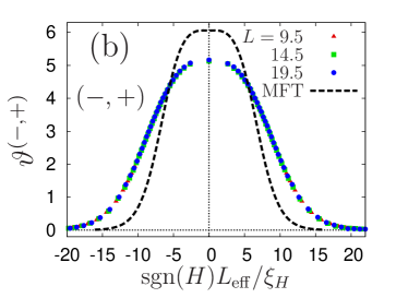
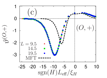
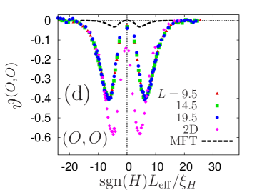
Figure 4: (a)-(d) show the same MC data as in Fig. 3, but not normalized. Here, the undetermined prefactor $g^{-1/2}$ of the MFT has has been fixed such that the depths of the minima in (a) are the same. This value of $g\simeq 187.5$ has been used for the MFT results in (b)-(d). For BC $(+,+)$ and $(O,O)$ (a) and (d) provide a comparison of the scaling functions in $d=4$ and 3 with those in $d=2$ MDC . The effect of stronger fluctuations in $d=2$ is most pronounced for free BC. In $d=2$ one has $\xi_{H,0}=0.233(1)$ ZMD .

It is instructive to compare these universal scaling functions for $d=3$ with those for $d=4$ which follow from minimizing the Landau-Ginzburg Hamiltonian corresponding to eq. (1) Diehl :

$$\begin{array}[]{c}\mathscr{H}=\tilde{A}\int\limits_{0}^{\tilde{L}}\left[\frac{1}{2}\left(\frac{{\mathrm{d}}\phi}{{\mathrm{d}}z}\right)^{2}+\frac{1}{2}\tau\phi^{2}+\frac{g}{4!}\phi^{4}-\tilde{H}\phi\right]dz+\\ +\tilde{A}\left[\frac{1}{2}c_{-}\phi_{0}^{2}-\tilde{H}_{1}^{-}\phi_{0}+\frac{1}{2}c_{+}\phi_{1}^{2}-\tilde{H}_{1}^{+}\phi_{L}\right],\end{array}$$ (8)

where $\exp\{-\mathscr{H}[\phi]\}$ is the statistical weight of the scalar order parameter field, $\tilde{A}$ is the three-dimensional cross-sectional area, $\tilde{L}$ is the film thickness, $g>0$, $\tilde{H}$ is the bulk field, $\tilde{H}_{1}^{-}$ and $\tilde{H}_{1}^{+}$ are bottom and top surface fields, $\phi_{0}=\phi(z=0)$, and $\phi_{L}=\phi(z=\tilde{L})$. Within mean field theory (MFT), $1/c_{i}$ $[i=-,+]$ are extrapolation lengths Diehl , $\tau=(\xi_{t,0}^{+})^{-2}t$ for $t>0$, and $\tau=(\sqrt{2}\xi_{t,0}^{+})^{-2}t$ for $t<0$. Here and below we use the tilde $\tilde{\rule{0.0pt}{4.0pt}}$ to mark MFT quantities. The solution of the corresponding Euler-Lagrange equation renders the equilibrium order parameter profile:

$$\frac{{\mathrm{d}}^{2}\phi}{{\mathrm{d}}z^{2}}-\tau\phi(z)-\frac{g}{6}\phi^{3}(z)+\tilde{H}=0$$ (9)

with the BC

$$\left.\frac{{\mathrm{d}}\phi}{{\mathrm{d}}\tilde{z}}\right|_{\tilde{z}=0}=c_{i}\phi(\tilde{z}=0)-\tilde{H}_{1}^{i}$$ (10)

where $\tilde{z}$ is the separation from the wall, i.e., $\tilde{z}=z$ for $-$ and $\tilde{z}=\tilde{L}-z$ for $+$. For large $\tilde{H}_{1}^{i}$, the leading behavior of $\phi(\tilde{z}\ll\tilde{L})$ is given by $\pm\sqrt{12/g}{\tilde{z}}^{-1}$ SHD which corresponds to $\pm$ BC. For large $c_{i}$ one has $\phi(\tilde{z}=0)\;=0$ corresponding to BC O.

The stress tensor is

$$T_{zz}(z,\tau,\tilde{H})=\frac{1}{2}\left(\frac{{\mathrm{d}}\phi}{{\mathrm{d}}z}\right)^{2}-\frac{1}{2}\tau\phi^{2}(z)-\frac{g}{4!}\phi^{4}(z)+\tilde{H}\phi(z),$$ (11)

so that the CCF in units of $\tilde{A}$ and $k_{\mathrm{B}}T$ equals

$$f_{c}(\tau,\tilde{H},\tilde{L})=T_{zz}(z_{0},\tau,\tilde{H})-T_{zz}^{b}(\tau,\tilde{H})$$ (12)

where $z_{0}$ is an arbitrary point $0\leq z_{0}\leq\tilde{L}$. The bulk contribution is

$$T_{zz}^{b}(\tau,\tilde{H})=-\frac{1}{2}\tau\phi^{2}_{b}-\frac{g}{4!}\phi^{4}_{b}+\tilde{H}\phi_{b}$$ (13)

with $\phi_{b}$ as the solution of $\tau\phi_{b}+\frac{g}{6}\phi^{3}_{b}=\tilde{H}$. For comparison, in Figs. 3 and 4 we plot also the results for the normalized scaling functions $\tilde{\vartheta}^{(BC)}/|\tilde{\Delta}_{+,+}|$ as a function of $\mathrm{sgn}(\tilde{H})\tilde{L}/\xi_{\tilde{H}}$, where $\xi_{\tilde{H}}=\frac{1}{\sqrt{3}}|\tilde{H}|^{-1/3}$. These functions describe the universal behavior in $d=4$.

The CCF for $(+,+)$ BC [see Figs. 3(a) and 4(a)] is attractive. In $d=3$ the scaling function has a minimum at $\mathrm{sgn}(H)L_{\mathrm{eff}}/\xi_{H}\simeq-13.3$ for which the direction of the bulk field is opposite to that of the surface fields. The depth of this minimum is ca. 20.2 times the value of the force at the critical point $(T_{c},H=0)$. This means that the critical Casimir attraction between colloids suspended in a critical solvent can be increased substantially by increasing the concentration of that component of the binary liquid mixture which is not preferentially adsorbed at the surfaces of the colloidal particles. For $(O,+)$ BC the force is attractive for strong, negative values of $H$ and repulsive for $H>0$ [see Figs. 3(c) and 4(c)]. The scaling functions for $(-,+)$ and $(O,O)$ BC are symmetric with respect to $H=0$. For $(-,+)$ BC the scaling function has a maximum at the critical point $H=0$ [see Figs. 3(b) and 4(b)]. The CCF for $(O,O)$ BC is weakly attractive; the corresponding scaling function in $d=3$ has two symmetric minima at $\mathrm{sgn}(H)L_{\mathrm{eff}}/\xi_{H}\simeq\pm 6.2$.

In summary, we have carried out the energy integration method in order to compute the bulk free energy density of the three-dimensional Ising model in the presence of a bulk magnetic field $H$. On this basis, by using a coupling parameter approach we have determined the scaling functions of CCF for slabs of thickness $L$ at the critical temperature $T=T_{\mathrm{c}}$ as a function of the scaling variable $\mathrm{sgn}(H)L_{\mathrm{eff}}/\xi_{H}$. The universal scaling functions have been computed for the four types $(+,+)$, $(-,+)$, $(O,+)$, $(O,O)$ of BC and have been compared with results in $d=4$ and in $d=2$ as far as available. At $T=T_{c}$, for all considered BC except $(-,+)$ the CCF attain their largest strength off two-phase coexistence, i.e., for $H\neq 0$.

References

(1)
M. E. Fisher and P. G. de Gennes, C. R. Acad. Sci. Paris Ser. B 287, 207
(1978).
(2) H. B. Casimir,
Proc. K. Ned. Akad. Wet. 51 793 (1948).
(3) M. Kardar, R. Golestanian,
Rev. Mod. Phys. 71, 1233 (1999).
(4) M. Krech, Casimir Effect in Critical Systems
(World Scientific, Singapore, 1994).
(5) J. G. Brankov, D. M. Dantchev, and N. S. Tonchev, The
Theory of Critical Phenomena in Finite-Size Systems - Scaling and Quantum
Effects (World Scientific, Singapore, 2000).
(6) A. Gambassi, J. Phys.: Conf. Ser. 161, 012037 (2009).
(7) M. N. Barber, in Phase Transitions and Critical Phenomena,
edited by C. Domb and J. L. Lebowitz (Academic, New York, 1983), Vol. 8,
p. 149.
(8) V. Privman, in Finite Size Scaling and Numerical Simulation of
Statistical Systems, edited by V. Privman (World Scientific, Singapore,
1990), p. 1.
(9) M. Fukuto, Y. F. Yano, and P. S. Pershan, Phys. Rev. Lett.
94, 135702 (2005).
(10)
C. Hertlein, L. Helden, A. Gambassi, S. Dietrich, and C. Bechinger, Nature
451, 172 (2008).
(11)
A. Gambassi, A. Maciołek, C. Hertlein, U. Nellen, L. Helden, C. Bechinger,
and S. Dietrich,
Phys. Rev. E 80, 061143 (2009).
(12)
O. Vasilyev, A. Gambassi, A. Maciołek, and S. Dietrich, EPL 80, 60009
(2007).
(13)
O. Vasilyev, A. Gambassi, A. Maciołek, and S. Dietrich,
Phys. Rev. E 79, 041142 (2009).
(14) M. Hasenbusch, Phys. Rev. E 87, 022130 (2013).
(15) H.W. Diehl, in
Phase Transitions and Critical Phenomena,
edited by C. Domb and J.L. Lebowitz (Academic, London, 1986), Vol. 10, p.76.
(16) U. Nellen, L. Helden, and C. Bechinger,
EPL 88, 26001 (2009).
(17) T. F. Mohry, A. Maciołek, and S. Dietrich, Phys. Rev. E 81,
061117 (2010).
(18) M. Hasenbusch, Phys. Rev. B 83, 134425 (2011).
(19)
O. Vasilyev, A. Maciołek, S. Dietrich
Phys. Rev. E 84, 041605 (2011).
(20) D. Beysens and D. Estéve,
Phys. Rev. Lett. 54, 2123 (1985).
(21) U. Nellen,
“Kolloidale Wechselwirkungen in binären Flüssigkeiten”,
doctoral thesis, University of Stuttgart (2011), available at
http://elib.uni-stuttgart.de/opus/volltexte/2011/6825/.
(22) F. Schlesener, A. Hanke, and S. Dietrich,
J. Stat. Phys. 110, 981 (2003).
(23) S. Buzzaccaro, J. Colombo, A. Parola, and R. Piazza,
Phys. Rev. Lett. 105, 198301 (2010).
(24)
R. Piazza, S. Buzzaccaro, A. Parola, and J. Colombo,
J. Phys.: Condens. Matter 23, 194114 (2011).
(25) T.F. Mohry, A. Maciołek, and S. Dietrich,
J. Chem. Phys. 136, 224902 (2012).
(26) A. Drzewiński, A. Maciołek, and A. Ciach,
Phys. Rev. E 61, 5009 (2000).
(27)
A. Maciołek, A. Drzewiński, and A. Ciach,
Phys. Rev. E 64, 026123 (2001).
(28)
A. Maciołek, A. Drzewiński, and R. Evans, Phys. Rev. E 64, 056137 (2001).
(29) A. Pelissetto and E. Vicari, Phys. Rep. 368, 549 (2002).
(30) R. Guida and J. Zinn Justin, J. Phys. A: Math. Gen. 31,
8103 (1998).
(31) C. Ruge, P. Zhu, and F. Wagner, Physica A 209, 431 (1994).
(32) M. E. Fisher and H. Nakanishi, J. Chem. Phys. 75, 5857 (1981).
(33) K. K. Mon, Phys. Rev. B 39, 467 (1989);
K. K. Mon and K. Binder, Phys. Rev. B 42, 675 (1990).
(34) A. Hucht, Phys. Rev. Lett. 99, 185301 (2007).
(35) M. Hasenbusch, Phys. Rev. B 82, 104425 (2010).
(36) M. Hasenbusch,
J. Stat. Mech., P07031 (2009).
(37) D. P. Landau and K. Binder, A Guide to Monte Carlo
Simulations in Statistical Physics (Cambridge University Press, London,
2005), p. 155.
(38) A. M. Ferrenberg and R. H. Swendsen,
Phys. Rev. Lett. 63, 1195 (1989).
(39) J. Engels, L. Fromme, and M. Seniuch,
Nucl. Phys. B 655, 277 (2003).
(40) M. Zubaszewska, A. Maciołek, and A. Drzewiński,
preprint arXiv:1308.6381 (2013).