Bayesian Inference in Sparse Gaussian Graphical Models

Abstract

One of the fundamental tasks of science is to find explainable relationships between observed phenomena. One approach to this task that has received attention in recent years is based on probabilistic graphical modelling with sparsity constraints on model structures. In this paper, we describe two new approaches to Bayesian inference of sparse structures of Gaussian graphical models (GGMs). One is based on a simple modification of the cutting-edge block Gibbs sampler for sparse GGMs, which results in significant computational gains in high dimensions. The other method is based on a specific construction of the Hamiltonian Monte Carlo sampler, which results in further significant improvements. We compare our fully Bayesian approaches with the popular regularisation-based graphical LASSO, and demonstrate significant advantages of the Bayesian treatment under the same computing costs. We apply the methods to a broad range of simulated data sets, and a real-life financial data set.

1 Introduction

Learning and exploiting structure in data is a fundamental machine learning problem. The notion of structure is closely related to sparsity. Indeed, to find structure often means to discover a sparse underlying graphical model. Learning a model structure, and incorporating prior structural knowledge, is important for prediction, knowledge discovery, and computational tractability, and has applications across multiple domains such as finance and systems biology.

A popular technique for learning sparse graphical models is to optimise an objective function with a penalty on the $L1$ norm of the parameters. This has been applied, for example, to regression (Tibshirani,, 1996), and to sparse coding (Olshausen and Field,, 1996). There has been considerable recent attention on Gaussian graphical models (GGMs), wherein the inverse covariance (precision) matrix reflects the structure: zeros in the precision correspond to missing edges in the model’s Markov random field. Therefore, the problem of structure learning in a GGM may be cast as the learning of a sparse precision matrix. Much recent work has been devoted to the MAP solution of an $L1$-constrained formulation of this problem (Meinshausen and Bühlmann,, 2006; Banerjee et al.,, 2008; Friedman et al.,, 2008; Duchi et al.,, 2008; Scheinberg et al.,, 2010); and its extensions to group sparsity (Friedman et al.,, 2010); handling non-Gaussianity (Liu et al.,, 2009); and incorporating latent variables (Agakov et al.,, 2012).

Bayesian methods may offer a more principled approach, but they are often considered to be much slower than optimisation methods. However, Mohamed et al., (2012) recently compared the $L1$ approach with Bayesian methods based on the “spike-and-slab” prior, focussing on unsupervised linear latent variable models. They found that the Bayesian methods could outperform $L1$, even when both were constrained by the same time budget. Here, we address the question of whether Bayesian methods can outperform the $L1$ optimisation approach to infer sparse precision matrices.

A class of Bayesian GGMs based on the GWishart distribution (see section 2.2) has been under development in parallel with the graphical lasso. See, for example, (Roverato,, 2002; Atay-Kayis and Massam,, 2005; Wang and Carvalho,, 2010; Dobra et al.,, 2010; Mitsakakis et al.,, 2011; Lenkoski and Dobra,, 2011; Dobra et al.,, 2011; Wang and Li,, 2012). Inference in these models is often limited by the efficiency with which the GWishart can be sampled. Wang and Li, (2012) demonstrate that the block Gibbs sampler is currently state of the art for this task. A more efficient sampler would make inference in GWishart-based models faster, and could make practical the use of more complex, higher-dimensional models. Hamiltonian Monte Carlo (HMC) samplers (see section 2.3) can facilitate fast mixing in distributions where the random variables are strongly coupled. Furthermore, they naturally take advantage of sparsity: the bottleneck in HMC is often the computation of the energy gradient with respect to the distribution parameters. Fewer parameters means fewer gradients to evaluate. In this paper, we develop an HMC approach to sample from the GWishart distribution.

The key contributions of the paper are as follows. First, we identify a simple modification of the block Gibbs sampler that makes it considerably more efficient when used as part of a high-dimensional GGM sampler. We then develop an HMC approach to sampling the GWishart, and demonstrate substantial gains in efficiency over block Gibbs methods. Finally, we utilise this sampler within a sparse Bayesian GGM, and show on a real-world data set that the model can outperform graphical lasso, even when the methods have the same time budget.

2 Background

2.1 Graphical Lasso

The inverse covariance (precision) matrix $\bm{\Lambda}$ of a Gaussian model $p(\bm{y})=\mathcal{N}(\bm{y}|\bm{\mu},\bm{\Lambda}^{-1})$ determines its graphical structure: zeros in $\bm{\Lambda}$ correspond to missing edges in the Markov random field. Therefore one may hope to learn the model structure by learning a sparse precision. One way to do this is to introduce $L1$ penalties on the elements of $\bm{\Lambda}$, and optimise the objective

$$\operatorname*{arg\,max}_{\bm{\Lambda}}\left[\log\det\bm{\Lambda}-\operatorname{tr}\left(\bm{S}\bm{\Lambda}\right)-\gamma\|\bm{\Lambda}\|_{1}\right],$$ (1)

where $\bm{S}$ is the empirical covariance, $\gamma$ is the penalty, and $\|\bm{\Lambda}\|_{1}=\sum_{i,j}|\Lambda_{ij}|$ is the $L1$ norm of $\bm{\Lambda}$. The optimum is the maximum a posteriori (MAP) solution for $\bm{\Lambda}$ with independent Laplace priors on its elements. The penalty $\gamma$ must be fixed in advance. Typically, this is done by cross-validation over some plausible range.

There has been much recent work on solving this problem efficiently; see, for example, (Meinshausen and Bühlmann,, 2006; Banerjee et al.,, 2008; Friedman et al.,, 2008; Duchi et al.,, 2008; Scheinberg et al.,, 2010). The approach of Friedman et al., (2008) was named the graphical lasso, and the problem itself is often referred to by the same name - as we do in this paper.

2.2 The GWishart Distribution

Let $G=(V,E)$ denote a graph. The GWishart $W_{G}(b,\bm{D})$ is a distribution over matrices $\bm{\Lambda}$ that respect the graph structure. Precisely, the density is:

$$p(\bm{\Lambda}|\bm{G})=\frac{1}{I_{G}(b,\bm{D})}|\bm{\Lambda}|^{\frac{b-2}{2}}\exp\left[-\frac{1}{2}\operatorname{tr}(\bm{D}\bm{\Lambda})\right]1_{[\bm{\Lambda}\in M^{+}(G)]}\ ,$$ (2)

where $b$ is the degrees of freedom, $\bm{D}$ is the scale matrix, $1_{[]}$ is the indicator function, $M^{+}(G)=\{\bm{\Lambda}\in S_{++}\mbox{ such that }\Lambda_{ij}=0\mbox{ if }(i,j)\notin E,i\neq j\}$, and $S_{++}$ is the cone of positive-definite matrices. Computing the normalisation constant $I_{G}(b,\bm{D})$ is not straightforward. It may be approximated by sampling (Atay-Kayis and Massam,, 2005) or by Laplace approximation (Lenkoski and Dobra,, 2011), for example.

Following the notation of Atay-Kayis and Massam, (2005), we define

$$\mathcal{V} =\{(i,j),i\leq j\ \mbox{such that either}\ i=j,i\in V\ \mbox{or}\ (i,j)\in E\},$$ (3)

$$\mathcal{W} =\{(i,j),i,j\in V,i\leq j\},$$ (4)

$$\bar{\mathcal{V}} =\mathcal{W}\setminus\mathcal{V}.$$ (5)

We define $\bm{\Lambda}^{\mathcal{V}}=\{\Lambda_{ij}:(i,j)\in\mathcal{V}\}$. We use $\bm{\Lambda}_{\mathcal{V}}$ to refer to a vectorised form of $\bm{\Lambda}^{\mathcal{V}}$.

Like the Wishart, the GWishart is the conjugate prior of the precision of a multivariate Gaussian. Let $\bm{y}\sim\mathcal{N}(0,\bm{\Lambda}^{-1})$, and let $\bm{Y}\in\mathbb{R}^{n\times p}$ be a data matrix. The posterior distribution of $\bm{\Lambda}$ is $W_{G}(b+n,\bm{D}+\bm{Y}^{T}\bm{Y})$.

2.3 Hamiltonian Monte Carlo

Hamiltonian Monte Carlo (HMC) (see, for example, (Neal,, 2010)) is an augmented-variable, MCMC approach to sampling. It can often result in rapid mixing in distributions with strong correlations between the random variables. Let $\bm{x}\in\mathbb{R}^{d}$ be a random vector with density $p(\bm{x})=Z^{-1}\exp(-E(\bm{x}))$, where $Z$ is a normalisation constant and $E(\bm{x})$ is the energy function. By physical analogy, one introduces the momentum vector $\bm{p}\in\mathbb{R}^{d}$ and constructs the Hamiltonian function

$$H(\bm{x},\bm{p})=E(\bm{x})+\frac{1}{2}\bm{p}^{T}\bm{M}^{-1}\bm{p},$$ (6)

where $\bm{M}$ is called the mass matrix. This is to be interpreted as the sum of a potential energy and a kinetic energy. By sampling from the joint density $p(\bm{x},\bm{p})\propto\exp(-H(\bm{x},\bm{p}))$ and discarding the momenta, one obtains samples from $p(\bm{x})$.

The procedure for updating the Markov chain is as follows. First, $\bm{p}$ is sampled from $\mathcal{N}(\bm{0},\bm{M})$. Then, a new value of $\bm{x}$ is proposed by simulating Hamiltonian dynamics, as defined by the equations

$$\dot{\bm{x}}=\bm{M}^{-1}\bm{p},\ \ \ \dot{\bm{p}}=-\nabla E(\bm{x}).$$ (7)

The leapfrog integrator is typically used to approximate the dynamics. Given a step size $\epsilon$ and current state $\left(\bm{x}_{0},\bm{p}_{0}\right)=\left(\bm{x}(t),\bm{p}(t)\right)$, the leapfrog algorithm generates a proposal $\left(\bm{x}_{1},\bm{p}_{1}\right)=\left(\bm{x}(t+L\epsilon),\bm{p}(t+L\epsilon)\right)$ by iterating the following updates for $L$ steps:

$$\bm{p}\left(\tau+\frac{\epsilon}{2}\right) =\bm{p}(\tau)-\frac{\epsilon}{2}\nabla E\left(\bm{x}(\tau)\right),$$ (8)

$$\bm{x}(\tau+\epsilon) =\bm{x}(\tau)+\epsilon\bm{M}^{-1}\bm{p}\left(\tau+\frac{\epsilon}{2}\right),$$ (9)

$$\bm{p}(\tau+\epsilon) =\bm{p}\left(\tau+\frac{\epsilon}{2}\right)-\frac{\epsilon}{2}\nabla E\left(\bm{x}(\tau+\epsilon)\right).$$ (10)

The parameters $(\epsilon,L)$ are chosen manually, typically by performing preliminary runs.

Finally, the proposal is accepted with probability $\min\{1,\exp(H(\bm{x}_{0},\bm{p}_{0})-H(\bm{x}_{1},\bm{p}_{1}))\}$, according to Metropolis-Hastings. This is necessary to correct for errors introduced by inexact simulation of the Hamiltonian dynamics.

3 Bayesian Inference in GWishart-Based Models

A number of sampling procedures have been invented to do inference in the GWishart distribution. Wang and Carvalho, (2010) developed a rejection sampler; Mitsakakis et al., (2011) developed a Metropolis-Hastings method in which the proposals are independent of previous samples; Dobra et al., (2011) demonstrated efficiency gains using a random-walk MCMC scheme in which each element of $\bm{\Lambda}^{\mathcal{V}}$ is updated conditioned on the other elements.

However, Wang and Li, (2012) demonstrated that a block Gibbs sampler (Piccioni,, 2000) convincingly outperforms other methods. We now describe the block Gibbs sampler, and suggest a simple modification to improve efficiency in high dimensions. We then introduce a novel HMC sampler. In the final part of this section, we describe a Bayesian sparse GGM in which these improvements can be utilised.

3.1 Sampling the GWishart with Block Gibbs

The GWishart block Gibbs sampler (Piccioni,, 2000; Wang and Li,, 2012) is based on the fact that a block of $\bm{\Lambda}$ corresponding to a clique in $G$ can be sampled conditional on the rest of $\bm{\Lambda}$ by sampling from a Wishart. Thus, given a set of cliques that cover $\bm{\Lambda}^{\mathcal{V}}$, a sampler for the GWishart can be constructed by iterating over the covering set and conditionally sampling each block of $\bm{\Lambda}$.

More precisely, the block Gibbs algorithm is as follows. First, construct a set $\mathcal{I}=\{\mathcal{I}_{k}:1\leq k\leq K\}$ where $\mathcal{I}_{k}\in V$ such that all $\mathcal{I}_{k}$ are cliques, and $\cup_{\mathcal{I}_{k}\in\mathcal{I}}\bm{\Lambda}_{\mathcal{I}_{k},\mathcal{I}_{k}}=\bm{\Lambda}^{\mathcal{V}}$. Then, generate the next sample in the Markov chain by iterating over $k$, and at each step draw $A\sim W\left(b,\bm{D}_{\mathcal{I}_{k},\mathcal{I}_{k}}\right)$, and set

$$\bm{\Lambda}_{\mathcal{I}_{k},\mathcal{I}_{k}}=A+\bm{\Lambda}_{\mathcal{I}_{k},V\setminus\mathcal{I}_{k}}\left(\bm{\Lambda}_{V\setminus\mathcal{I}_{k},V\setminus\mathcal{I}_{k}}\right)^{-1}\bm{\Lambda}_{V\setminus\mathcal{I}_{k},\mathcal{I}_{k}}.$$ (11)

The choice of covering set $\mathcal{I}$ can have a significant effect on the performance of the sampler, and the optimal choice probably depends on $G$. Wang and Li, (2012) considered two choices for $\mathcal{I}$: (1) The maximal cliques; (2) All pairs of nodes connected by an edge, plus all isolated nodes. It was found that maximal cliques gave better performance than the edgewise covering set in all the models considered. However, it seems likely that the set of all maximal cliques will be a suboptimal choice in many models. First, finding the maximal cliques is NP-hard, so this method may scale poorly. Second, the number of maximal cliques may be much greater than that required to cover $\bm{\Lambda}^{\mathcal{V}}$; a smaller covering set may trade off a little mixing quality for a significant speed up.

In this paper, we investigate this with a simple heuristic to build $\mathcal{I}$. It is motivated by the desire to build large cliques to facilitate mixing, but to keep the number of cliques small to reduce run time. The algorithm is as follows. First, randomly permute the nodes $V$, and permute the matrix $\bm{G}$ accordingly. Then, iterate over the entries of $\bm{G}$; for each non-zero $G_{ij}$ not yet included in any clique $\mathcal{I}_{k}$, build a maximal clique starting with $\{i,j\}$. Grow this clique by considering nodes in the permuted order, and add them greedily. So, rather than finding all maximal cliques, this algorithm quickly finds a small covering set of maximal cliques, which should improve the efficiency of the block Gibbs sampler in high dimensional models.

3.2 Sampling the GWishart with HMC

We develop an HMC method to sample from the GWishart distribution. We now describe the key choices and challenges to make it work well: dealing with the positive-definite constraint on the precision, choosing the step size and path length parameters, and adapting the mass matrix.

3.2.1 The Positive-Definite Constraint

The GWishart $W_{G}(b,\bm{D})$ is a distribution over positive-definite matrices $\bm{\Lambda}\in M^{+}(G)$. When running HMC, we must ensure that $\bm{\Lambda}$ remains within the positive-definite cone $S_{++}$. Naively, this may be done by simply setting the energy to infinity outside $S_{++}$. However, this may lead to a high rejection rate if the approximate dynamics often lead to proposals outside the cone. When $b>2$, the energy approaches infinity at the boundary, so the chain would remain in $S_{++}$ if the dynamics could be simulated exactly. But in practice, the leapfrog method can overshoot the boundary. For $b\leq 2$, the situation is worse as even the exact dynamics lead the chain outside $S_{++}$.

One idea is to reflect the simulated path off the constraint boundary, which is straightforward when the constraints are simply bounds on each variable. But for the positive-definite constraint, it is non-trivial to find where the path crosses the boundary, or to find the tangent plane at that point. Another idea is to use the linearly transformed Cholesky decomposition (Atay-Kayis and Massam,, 2005)

$$\bm{D}^{-1}=\bm{T}^{T}\bm{T};\ \ \bm{\Lambda}=\bm{\Phi}^{T}\bm{\Phi};\ \ \bm{\Psi}=\bm{\Phi}\bm{T}^{-1},$$ (12)

in which the free variables are $\bm{\Psi}^{\mathcal{V}}$. The non-free variables $\bm{\Psi}^{\bar{\mathcal{V}}}$ are functions of the free elements that precede them in a row-wise ordering. If HMC is applied in this representation, there are no constraints on $\bm{\Psi}^{\mathcal{V}}$. However, the energy gradient with respect to each free $\Psi_{ij}^{\mathcal{V}}$ depends on the gradients preceding it in the row-wise ordering. So the gradients must be evaluated sequentially, which makes HMC very slow.

Step Size and Trajectory Length

Instead, we run HMC in $\bm{\Lambda}$-space. We find that judicious choices of the step size and trajectory length are sufficient to acheive good performance. We draw $\epsilon$ from a distribution that concentrates much of its mass near the mean, yet still results in the occasional draw of a very small value. The intuition is that this should facilitate good mixing, while still allowing the chain to move away from the $S_{++}$ boundary by using a small step size (and therefore simulating the dynamics accurately). We choose a fixed target trajectory length $L=\max\left(1,\lfloor\beta/\epsilon\rceil\right)$, where $\beta$ is a user-defined parameter, so that when a small $\epsilon$ is chosen, the chain still moves a long distance. With a fixed trajectory length, the distribution of $\epsilon$ cannot have too much mass near zero, or the sampler will be slow. This rules out the exponential distribution, for example. In this paper, we use a $\Gamma(2,\alpha)$ distribution. The parameters $(\alpha,\beta)$ are chosen by performing preliminary runs (as is typical in HMC).

We find this method, in combination with a well-chosen mass matrix, performs well provided the degrees of freedom parameter $b$ is greater than 10 or so. This is almost always the case for a posterior GWishart because $b$ increases with the number of data points. But this HMC approach may not be the best choice for GWishart priors with small $b$.

3.2.2 The Mass Matrix

To sample from the GWishart distribution, we run HMC on the random vector $\bm{\Lambda}_{\mathcal{V}}$. We find that the choice of mass strongly influences its performance. One approach to selecting a mass matrix is to estimate the covariance $\bm{\Sigma}$ of this random vector and set $\bm{M}=\bm{\Sigma}^{-1}$ (Neal,, 2010). We considered the following methods for estimating $\bm{\Sigma}^{-1}$, which we compare experimentally in section 4.2.

1. Set $\bm{\Sigma}$ to the identity matrix.

2. Perform a short block Gibbs run and set $\bm{\Sigma}$ to the empirical covariance.

3. Compute a Laplace approximation to the distribution of $\bm{\Lambda}_{\mathcal{V}}$, and set $\bm{\Sigma}$ to its covariance.

4. Assume $\bm{\Lambda}\sim W(b,\bm{D})$, draw samples from the Wishart, and compute the empirical precision $\bm{K}$ of $\bm{\Lambda}_{\mathcal{W}}$. Then set $\bm{\Sigma}^{-1}=\bm{K}_{\mathcal{V},\mathcal{V}}$. This corresponds to a Gaussian approximation on the distribution of $\bm{\Lambda}_{\mathcal{W}}$ - an approximation which was shown to become more accurate as $b$ increases (Lenkoski and Dobra,, 2011).

3.3 A Sparse Bayesian GGM

Consider the following spike-and-slab GGM:

$$\bm{G}\sim P(\bm{G});\ \ \bm{\Lambda}\sim W_{G}(b,\bm{D});\ \ \bm{y}\sim\mathcal{N}(0,\bm{\Lambda}^{-1}).$$ (13)

$P(\bm{G})$ is an arbitrary distribution on graphs, but is typically something simple such as the uniform distribution or a product of Bernoulli distributions on the edges. This model has received considerable attention in recent years; see, for example (Dobra et al.,, 2011; Rodriguez et al.,, 2011; Dobra and Lenkoski,, 2011; Wang and Li,, 2012).

Bayesian inference in this model typically involves sampling. One of the most efficient of such existing methods (Wang and Li,, 2012), which we refer to as WL, iterates two steps: the first samples $\bm{\Lambda}$ given $\bm{G}$ and $\bm{Y}$, and the second makes changes to the graph structure. The first step is to sample from a GWishart. In the second step, sampling $\bm{G}$ is done using a double Metropolis-Hastings method (Liang,, 2010) with a reversible jump step. Wang and Li, (2012) propose to flip one edge at a time, then resample the precision from its prior, before accepting or rejecting the transition according to Metropolis-Hastings. The efficiency of WL depends strongly on the efficiency of the GWishart sampler. In this paper, we improve on existing methods using our HMC technique.

In section 4.3, we compare the performance of this model against graphical lasso on a real-world data set, where each model is allocated the same time budget.

4 Experiments

4.1 HMC versus Block Gibbs

We compare HMC and block Gibbs on synthetically generated data, testing the effects of dimensionality, data size, and sparsity on the efficiency of these samplers. Each test case corresponds to a setting of the model dimensionality $p$; a sparsity parameter $s$ where $0\leq s\leq 1$; and the ratio $n/q$, where $n$ is the number of data points and $q$ is the expected number of free variables.

Each test case is composed of 10 runs. In each run, a graph $G$ is drawn by sampling each edge from $Bern(s)$, and a precision matrix $\bm{\Lambda}$ is drawn from $W_{G}\left(1,p\bm{I}_{p}\right)$ by taking the $1000^{th}$ sample from a block Gibbs run. The $n$ data points are then drawn from $\mathcal{N}\left(\bm{0},\bm{\Lambda}^{-1}\right)$.

We sample from the posterior of each test run using HMC in which the mass matrix is computed by sampling from a (fully connected) Wishart distribution and then conditioning on the missing edges as described in section 3.2.2. We compare this to the block Gibbs sampler in which the covering set of cliques is generated in two different ways: (1) BG-MC: the covering set consists of all maximal cliques; (2) BG-HCC: our heuristic clique cover algorithm (see section 3.1).

For all samplers, $\bm{\Lambda}$ is initialised to the identity matrix. We ran 100 iterations of burn-in, and then gathered the following 10000 samples. Table 1 shows the results.

Table 1: Comparison by ESS/sec on synthetic data of HMC and two block Gibbs methods: BG-MC, where the covering set consists of all maximal cliques; and BG-HCC, our heuristic clique cover algorithm. Block Gibbs is best only for very low-dimensional models. HMC is orders of magnitude faster in higher dimensions.

Test		BG-MC		BG-HCC		HMC
Dimension	$p$	ESS	ESS/sec	ESS	ESS/sec	ESS	ESS/sec
	10	7697 (1161)	878 (136)	7086 (1173)	529 (100)	10000 (0)	514 (10)
$n/q=5$	25	4087 (1051)	39.9 (12.3)	1525 (625)	20.0 (8.2)	10000 (0)	244 (4)
$s=0.5$	50	3037 (693)	1.59 (0.5)	521 (240)	1.26 (0.58)	9977 (74)	61.8 (3.6)
	75	-	-	188 (81)	0.151 (0.068)	9999 (1)	16.6 (0.6)
	100	-	-	150 (76)	0.0624 (0.0360)	8836 (317)	3.62 (0.18)
Data size	$n/q$	ESS	ESS/sec	ESS	ESS/sec	ESS	ESS/sec
	0.2	4435 (439)	26.3 (4.1)	1910 (425)	24.8 (5.3)	7704 (431)	83.9 (5.5)
$p=25$	1	4060 (1158)	24.6 (8.4)	1905 (877)	26.2 (14.8)	9990 (16)	235 (34)
$s=0.5$	5	3809 (1084)	23.1 (7.2)	1681 (640)	23.2 (9.9)	10000 (0)	295 (4)
	25	3534 (733)	20.8 (4.6)	1254 (453)	16.8 (6.2)	9929 (212)	324 (10)
	100	3020 (898)	18.8 (5.9)	1185 (601)	15.7 (8.4)	9554 (1128)	314 (38)
Sparsity	$s$	ESS	ESS/sec	ESS	ESS/sec	ESS	ESS/sec
	0.1	8221 (1376)	147 (34)	8221 (1431)	146 (35)	10000 (0)	316 (19)
$p=25$	0.25	3177 (767)	33.7 (8.7)	2700 (763)	32.2 (9.5)	10000 (0)	254 (6)
$n/q=5$	0.5	3089 (1423)	14.4 (6.8)	1108 (842)	12.6 (10.2)	9995 (13)	239 (7)
	0.75	7439 (776)	14.2 (1.7)	1933 (450)	27.1 (5.2)	10000 (0)	214 (6)
	0.9	9426 (179)	21.1 (12.7)	4995 (1221)	96.3 (34.4)	10000 (0)	205 (21)

Times do not include the time taken to compute the index sets in block Gibbs, or to compute the mass matrix in HMC. When $\bm{G}$ is fixed as in this experiment, these times are negligible. (But if the sampler is to be part of a joint sampler for $(\bm{G},\bm{\Lambda})$, then they are significant, as discussed in sections 4.2 and 4.3).

There are missing entries for BG-MC at dimensionalities 75 and 100: we abandoned those tests because they were taking an extremely long time. We consider BG-MC to be impractical for high-dimensional problems. BG-HCC is more efficient than BG-MC in this scenario, and also when the sparsity is such that BG-MC has to work with a large number of maximal cliques.

The table shows that BG-MC is best for low dimensional models, but when $p\geq 25$, HMC is significantly more efficient. The effect of the data size is different for block Gibbs and HMC. Block Gibbs tends to improve as data size decreases; HMC tends to improve with more data, we expect because the Gaussian approximation used when computing the mass matrix becomes more accurate. As the graph becomes sparser ($s$ decreases), HMC improves because there are fewer variables to simulate. The block Gibbs methods tend to prefer either very sparse or very dense graphs, which is expected because these cases will usually produce fewer cliques than a moderate level of sparsity.

In summary: (1) For block Gibbs, using BG-HCC is preferable to BG-MC in high dimensions, or when the level of sparsity is unfavourable to BG-MC; (2) Except for the 10-dimensional case, HMC performs significantly better than both block Gibbs methods across all our tests.

4.2 Comparing Methods of Computing the Mass Matrix

We compared the methods of computing the mass matrix described in section 3.2.2. We generated 10 runs of a single test case as in section 4.1. The parameters were: $p=25,n/q=5,s=0.5$. We sampled the distributions using each of the mass matrix methods. For the two methods requiring preliminary samples, we drew 20000 points. For the Laplace approximation, we found the mode numerically by gradient ascent.

The results are shown in Table 2.

Table 2: Comparison of methods for computing the HMC mass matrix.

	Identity	Prelim. GWishart	Laplace	Prelim. Wishart
Time to compute M (s)	0 (0)	91.6 (13.3)	27.1 (23.1)	2.15 (0.04)
Sampling time (s)	5560 (316)	21.7 (0.2)	18.3 (0.8)	21.8 (0.3)
ESS	2348 (726)	10000 (0)	669 (470)	10000 (0)
ESS/sec	0.425 (0.138)	461 (3)	37.0 (25.9)	460 (7)

Clearly, the identity matrix mass makes HMC highly inefficient. The Laplace approximation also performed quite poorly. In terms of ESS/sec, a preliminary sampling run from the GWishart, and from the Wishart (followed by conditioning on missing edges), gave similar results. However, the preliminary run is considerably more expensive on the GWishart. If the HMC sampler is to be embedded in a joint sampler for $(\bm{G},\bm{\Lambda})$, the preliminary GWishart run needs to be repeated each time the graph changes, which is clearly impractical. But the precision $\bm{K}$ computed from the Wishart samples remains valid as the graph changes: the new mass can be obtained simply by removing those rows and columns from $\bm{K}$ that correspond to missing edges.

4.3 The Bayesian Sparse GGM versus Graphical Lasso

Having demonstrated the advantages of using an HMC sampler over block Gibbs for the GWishart, we now employ this method in the Bayesian sparse GGM model, and compare this model with the frequentist graphical lasso on a real-world data set. Our data consist of the daily closing prices of 35 stocks from 7 market sectors of the FTSE100 index on 1000 days over the period from 2005 to 2009. The price data were cleaned and converted to returns by computing the ratio of closing prices on consecutive days. The first 500 points were used for training, leaving 500 points in the test set. We preprocessed the data by subtracting the mean, and scaling such that the empirical precision had all ones along the main diagonal.

It is well known that equity returns are not Gaussian-distributed. But for purposes of comparison, we applied both the Bayesian GGM methods and the graphical lasso to this data set. To set the penalty parameter $\gamma$ for graphical lasso, we did 5-fold cross-validation over 100 equally spaced values. We trained a model with the best-performing $\gamma$ and evaluated it via log likelihood of the test data.

For the Bayesian GGM, we use the WL method (see section 3.3) to sample $(\bm{G},\bm{\Lambda})$ jointly. We set $p(\bm{G}|s)=\prod_{i<j}s^{G_{ij}}(1-s)^{(1-G_{ij})}$, and introduce a sampling step to sample the hyperparameter $s$ (which is analogous to the L1 penalty in the graphical lasso). We found that the choice of parameters for the GWishart prior had little effect on the generalisation performance of the model. We report results for the prior $W_{G}(1+n_{0},(p+n_{0})\bm{I}_{p})$, where $n_{0}=10$.

The WL sampler requires samples from both the GWishart prior and posterior, and its performance depends strongly on the efficiency of this component. We test both BG-HCC and HMC for this task. BG-MC is far too slow to use within the WL sampler: when we tried it, WL could not complete a single iteration in the time it took to complete cross-validation on the graphical lasso. Most of the time is spent recomputing the maximal cliques each time the graph changes; but there are many maximal cliques, so lots of time is spent sampling too. For HMC, our results do not include the time taken to find good settings of the step parameters $(\alpha,\beta)$. We set these values by adjusting them such that the acceptance rate on preliminary runs is around 65% - as suggested by Neal, (2010) - and such that the ESS is high. In practice, little adjustment is needed because our choice of mass matrix means that similar step parameters can be used for a wide variety of GWishart distributions.

To make a comparison with graphical lasso, we approximate the expected test log likelihood $\langle\log p(\bm{Y}_{(test)}|\bm{\Lambda})\rangle_{p(\bm{\Lambda}|\bm{Y}_{(train)})}\approx N^{-1}\sum_{i=1}^{N}\log p\left(\bm{Y}_{(test)}|\bm{\Lambda}^{(i)}\right)$, using the samples $\bm{\Lambda}^{(i)}$ drawn from the posterior $p(\bm{\Lambda}|\bm{Y}_{(train)})$. We compute this expectation after each sample is drawn; Figure 1(a) shows how the value evolves over time for both the HMC and BG-HCC versions of the joint sampler for a typical run. The samplers do not quite agree because neither has yet converged. But right from the start, they perform significantly better than graphical lasso, which takes a few minutes to register its result. At the time graphical lasso finishes, the test log likelihood scores are: HMC $=(-5.19\pm 0.33)\times 10^{4}$; BG-HCC $=(-5.38\pm 0.35)\times 10^{4}$; GLASSO $=(-6.28\pm 0.51)\times 10^{4}$. For comparison, the test log likelihood under a Gaussian model with the empirical precision of the training data is $(-7.20\pm 0.70)\times 10^{4}$.

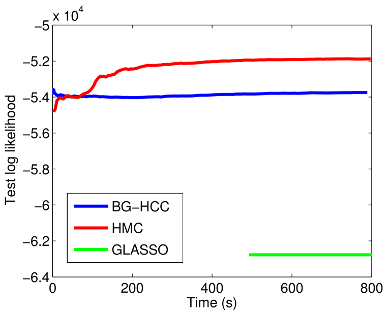
(a) Estimated test log likelihoods over time. The Bayesian methods result in significantly higher test log likelihoods - good estimates of which are obtained after only a few samples.

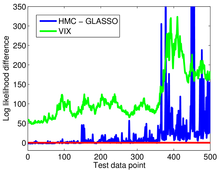
(b) For each point in the test data set, the difference in log likelihood between the Bayesian GGM and graphical lasso is plotted in blue. The VIX volatility index, arbitrarily scaled to fit, is in green. The Bayesian method performs better over the whole test set, but tends to strongly outperform graphical lasso when market volatility is high.

Figure 1: Comparison of the Bayesian GGM and graphical lasso on the FTSE data set.

Figure 1(b) offers an explanation for the better performance of the Bayesian models. It plots the difference in log likelihood for each point in the test set. The VIX index - which is a measure of market volatility - is overlayed. The graph shows that the Bayesian GGM fares particularly well against the graphical lasso when the market is more volatile. This seems likely to be a result of the Bayesian methods making use of the full posterior, rather than just using the MAP solution.

5 Discussion and Future Work

We have developed a Hamiltonian Monte Carlo sampler for the GWishart distribution and demonstrated its increased efficiency over the block Gibbs sampler. Our method - in particular, the choice of mass matrix - is suitable for embedding into a joint sampler of the graph and precision in a sparse Gaussian model. We also described a way to choose the covering set in the block Gibbs sampler that reduced run time and made it more practical to use this method within a joint sampler.

We then compared a sparse Bayesian GGM model based on the GWishart distribution with the graphical lasso estimator on a real-world data set. We found that the Bayesian model performed better in terms of test log likelihood, even when the models were constrained to the same time budget. The better performance of the Bayesian model appeared due to its use of the full posterior - as opposed to the graphical lasso’s MAP solution.

Future work could investigate other ways to set the mass matrix, or to select the step parameters, so as to further improve efficiency. It would also be interesting to extend the GGM model to incorporate latent variables, analogous to how Agakov et al., (2012) extended the graphical lasso. It would be harder to choose a useful mass matrix in that case, because the local geometry would change significantly over the space of joint precision matrices. Latent variables would also introduce multiple equivalent modes that may be hard for the sampler to traverse. Another possible direction is to allow the graph structure or precision matrix distributions to depend on side information. For example, in the experiment of section 4.3, market volatility may influence the dependence structure between the equities. This could be modelled by allowing the VIX to influence the graph distribution.

Acknowledgments

Peter Orchard wishes to thank Yichuan Zhang and Iain Murray for helpful discussions - especially those long discussions with Yichuan regarding HMC.

References

- Agakov et al., (2012) Agakov, F. V., Orchard, P. R., and Storkey, A. (2012). Discriminative Mixtures of Sparse Latent Fields for Risk Management. In AISTATS.
- Atay-Kayis and Massam, (2005) Atay-Kayis, A. and Massam, H. (2005). A Monte Carlo Method for Computing the Marginal Likelihood in Nondecomposable Gaussian Graphical Models. Biometrika, 92(2):317–335.
- Banerjee et al., (2008) Banerjee, O., El Ghaoui, L., and d’Aspremont, A. (2008). Model Selection through Sparse Maximum Likelihood Estimation for Multivariate Gaussian or Binary Data. The Journal of Machine Learning Research, 9:485–516.
- Dobra et al., (2010) Dobra, A., Eicher, T. S., and Lenkoski, A. (2010). Modeling Uncertainty in Macroeconomic Growth Determinants using Gaussian Graphical Models. Statistical Methodology, 7(3):292–306.
- Dobra and Lenkoski, (2011) Dobra, A. and Lenkoski, A. (2011). Copula Gaussian Graphical Models and their Application to Modeling Functional Disability Data. The Annals of Applied Statistics, 5(2A):969–993.
- Dobra et al., (2011) Dobra, A., Lenkoski, A., and Rodriguez, A. (2011). Bayesian Inference for General Gaussian Graphical Models with Application to Multivariate Lattice Data. Journal of the American Statistical Association, 106(496):1418–1433.
- Duchi et al., (2008) Duchi, J., Gould, S., and Koller, D. (2008). Projected Subgradient Methods for Learning Sparse Gaussians. In UAI, pages 145–152.
- Friedman et al., (2008) Friedman, J., Hastie, T., and Tibshirani, R. (2008). Sparse Inverse Covariance Estimation with the Graphical Lasso. Biostatistics, 9(3):432–441.
- Friedman et al., (2010) Friedman, J., Hastie, T., and Tibshirani, R. (2010). Applications of the Lasso and Grouped Lasso to the Estimation of Sparse Graphical Models. Technical report, Stanford University.
- Lenkoski and Dobra, (2011) Lenkoski, A. and Dobra, A. (2011). Computational Aspects Related to Inference in Gaussian Graphical Models with the G-Wishart Prior. Journal of Computational and Graphical Statistics, 20(1):140–157.
- Liang, (2010) Liang, F. (2010). A Double Metropolis-Hastings Sampler for Spatial Models with Intractable Normalizing Constants. Journal of Statistical Computation and Simulation, 80(9):1007–1022.
- Liu et al., (2009) Liu, H., Lafferty, J., and Wasserman, L. (2009). The Nonparanormal: Semiparametric Estimation of High Dimensional Undirected Graphs. J. Mach. Learn. Res., 10:2295–2328.
- Meinshausen and Bühlmann, (2006) Meinshausen, N. and Bühlmann, P. (2006). High-Dimensional Graphs and Variable Selection with the Lasso. The Annals of Statistics, 34(3):1436–1462.
- Mitsakakis et al., (2011) Mitsakakis, N., Massam, H., and D Escobar, M. (2011). A Metropolis-Hastings Based Method for Sampling from the G-Wishart Distribution in Gaussian Graphical Models. Electronic Journal of Statistics, 5:18–30.
- Mohamed et al., (2012) Mohamed, S., Heller, K., and Ghahramani, Z. (2012). Bayesian and L1 Approaches for Sparse Unsupervised Learning. In Langford, J. and Pineau, J., editors, Proceedings of the 29th International Conference on Machine Learning (ICML-12), ICML ’12, pages 751–758, New York, NY, USA. Omnipress.
- Neal, (2010) Neal, R. (2010). MCMC using Hamiltonian Dynamics in S. Brooks, A. Gelman, G. Jones, and X. Meng (Ed.), Handbook of Markov Chain Monte Carlo, Chapman & Hall.
- Olshausen and Field, (1996) Olshausen, B. A. and Field, D. J. (1996). Emergence of Simple-Cell Receptive Field Properties by Learning a Sparse Code for Natural Images. Nature, 381:607–609.
- Piccioni, (2000) Piccioni, M. (2000). Independence Structure of Natural Conjugate Densities to Exponential Families and the Gibbs’ Sampler. Scandinavian Journal of Statistics, 27:111–127.
- Rodriguez et al., (2011) Rodriguez, A., Lenkoski, A., and Dobra, A. (2011). Sparse Covariance Estimation in Heterogeneous Samples. Electronic Journal of Statistics, 5:981–1014.
- Roverato, (2002) Roverato, A. (2002). Hyper Inverse Wishart Distribution for Non-decomposable Graphs and its Application to Bayesian Inference for Gaussian Graphical Models. Scandinavian Journal of Statistics, 29(3):391–411.
- Scheinberg et al., (2010) Scheinberg, K., Ma, S., and Goldfarb, D. (2010). Sparse Inverse Covariance Selection via Alternating Linearization Methods. In Lafferty, J., Williams, C., Shawe-Taylor, J., Zemel, R., and Culotta, A., editors, Advances in Neural Information Processing Systems 23, pages 2101–2109.
- Tibshirani, (1996) Tibshirani, R. (1996). Regression Shrinkage and Selection via the Lasso. Journal of the Royal Statistical Society: Series B (Statistical Methodology), 58(1):267–288.
- Wang and Carvalho, (2010) Wang, H. and Carvalho, C. M. (2010). Simulation of Hyper-Inverse Wishart Distributions for Non-Decomposable Graphs. Electronic Journal of Statistics, 4:1470–1475.
- Wang and Li, (2012) Wang, H. and Li, S. Z. (2012). Efficient Gaussian Graphical Model Determination Under G-Wishart Prior Distributions. Electronic Journal of Statistics, 6:168–198.