Majorana fermions coupled to electromagnetic radiation

Abstract

We consider a voltage-biased Josephson junction between two nanowires hosting Majorana zero modes which occur as topological protected zero-energy excitations at the junction. We show that two Majorana fermions localized at the junction, even though being neutral particles, interact with the electromagnetic field and generate coherent radiation similar to the conventional Josephson radiation. Within a semiclassical analysis of the radiation field, we find that the optical phase gets locked to the superconducting phase difference and that the radiation is emitted at half the Josephson frequency. In order to confirm the coherence of the radiation, we study correlations of the radiation emitted by two spatially-separated junctions in a d.c.-SQUID geometry taking into account decoherence due to spontaneous state-switches as well as due to quasi-particle poisoning.

1 Introduction

Ever since its discovery, superconductivity has been of great importance for the understanding of quantum coherence. A particular example is the Josephson effect which in the most simple terms can be understood as a reactive current which is driven by a gradient of the superconducting phase and thus establishes the macroscopic coherence of the latter [1]. In fact, most of the physical phenomena related to superconducting tunnel junctions are governed by the Josephson equations which have their microscopic origin in a coherent transfer of Cooper pairs through the thin barrier. These equation predict that microwave radiation, also called Josephson radiation, is produced by a voltage biased tunnel junction [1, 2]. The microwave radiation is emitted coherently at the Josephson frequency $\omega_{{\scriptscriptstyle\rm J}}=2eV/\hbar$ which is given by twice the voltage bias $V$ that is applied across the junction [3, 4]; here and below, $e>0$ denotes the elementary charge. With superconducting-semiconducting hybrid devices, it is possible to imprint superconducting correlations onto semiconducting nano-devices like quantum dots or quantum wires [5]. Recently, the potential for the emergence of Majorana fermions in such hybrid systems has attracted a lot of interest in condensed matter physics [6, 7]. With an appropriate tuning of the physical parameters, Majorana zero modes are expected to appear as end states at the chemical potential of the superconductor [8, 9, 10, 11]. In particular, they are predicted to occur in one-dimensional semiconducting quantum wires in proximity to a conventional s-wave superconductor subject to a moderate magnetic field [12, 13]. In fact, recent experimental works seem to be in agreement with these predictions [14, 15, 16, 17]. In contrast to conventional Josephson junctions, single electrons can be transferred coherently in the presence of Majorana zero modes [18] leading to a $4\pi$-periodic current-phase relationship [8]. Because of this, the Josephson effect is dubbed fractional Josephson effect [8, 19] and its observation would provide a clear evidence of Majorana fermions.

The a.c. fractional Josephson effect was introduced in [20] and describes the case of voltage biased Josephson junctions with fractional supercurrents, see also [21, 22, 23] for detailed discussion of the a.c. effect. As a consequence, non-trivial Shapiro-steps with doubled height in the current-voltage relation emerge providing a signature of the Majorana fermions [24, 25, 15]. Regarding the interaction of Majorana zero modes with electromagnetic fields, it has been recently shown that Majorana fermions can be manipulated by means of microwave driving through weak coupling of microwave radiation to the states of a two Majorana wires [26]. Furthermore, in [27] the influence of Majorana fermions on the photon coupling of a Majorana-transmon qubit has been investigated.

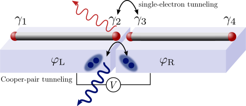
Figure 1: Two bulk s-wave superconductors (blue cuboids) forming a Josephson junction with superconducting phase difference $\varphi=\varphi_{{\scriptscriptstyle\rm L}}-\varphi_{{\scriptscriptstyle\rm R}}$. On top of each of them, there is a semiconducting nanowire (gray cylinders) in the topological phase supporting two Majorana fermions (red spheres) at its ends. We consider the case where the Josephson junction is voltage-biased such that Cooper pairs which move across the junction emit radiation at the Josephson frequency $2eV/\hbar$ with $V$ the voltage applied. This process is indicated by the bold wavy line. Due to the presence of the Majorana fermions, there is the additional process allowed which proceeds via the tunneling of a single unpaired electrons together with the emission of radiation at at half the Josephson-frequency indicated by the thin wavy line. In this paper, we will concentrate on the latter process.

In this work, we want to focus on the radiation that arises from coupling Majorana fermions to the electromagnetic field in a voltage-biased situation. In analogy to the common a.c. Josephson effect we show that the Majorana-induced Josephson radiation is coherent radiation with a frequency that is half of the Josephson frequency. Furthermore, there is a mutual relationship between the emitted radiation and the state of the Majorana fermions. As a consequence, the system exhibits correlations between the radiation fields emitted from different sources that are situated far away from each other. We will first introduce the coupling of the Majorana zero modes with the electromagnetic field. Then, we proceed outlining different possible realizations of a voltage biased fractional Josephson junction. Subsequently, we derive the semiclassical equation governing the radiation field when the junction is placed in a cavity. Moreover, we will discuss the steady state solution and possible decoherence mechanisms. We will finish with the discussion of correlations of spatially separated radiation sources and show that the superconducting coherence is partially imprinted onto the radiation field. In this respect, the system is closely related to prior work [28, 29, 30, 31] which we will discuss in details below.

2 Josephson radiation from Majorana fermions

2.1 Dipole coupling of Majorana fermions

In topological superconductors, Majorana fermions denoted by $\gamma_{j}$ appear as quasi-particles in the middle of the gap. Due to the build-in particle-hole symmetry of superconductors in the mean field description these solutions of the Bogoliubov-de Gennes equation are made-up from equal superpositions of electrons and holes,

$$\gamma_{j}=\int\left[w^{*}_{j}(\bm{r})\psi(\bm{r})+w_{j}(\bm{r})\psi^{\dagger}(\bm{r})\right]\,d^{3}r,$$ (1)

where $\psi(\bm{r})$ denotes the fermionic field operator of the electrons and $w(\bm{r})$ is the wave function of a zero energy solutions of the Bogoliubov-de Gennes equation which is localized at either end of the nanowire [8, 12, 13]. The Majorana operators obey the Clifford algebra $\{\gamma_{j},\gamma_{k}\}=2\delta_{jk}$. In case the wire is manufactured on top of a Josephson junction additional Majorana fermions have to be taken into account on either side of the Josephson junction [19]. Accordingly, we consider four Majorana bound states in the system denoted by $\gamma_{1},\ldots,\gamma_{4}$, cf. figure 1. For the further analysis, it is convenient to introduce two conventional fermionic operators

$$f_{{\scriptscriptstyle\rm L}} =\frac{1}{2}\left(\gamma_{1}+i\gamma_{2}\right),\qquad f_{{\scriptscriptstyle\rm R}}=\frac{1}{2}\left(\gamma_{3}+i\gamma_{4}\right).$$ (2)

These fermionic operators account for the parity of the number of electrons on either side of the Josephson junction with the parity given by $\mathcal{P}_{x}=(-1)^{f^{\dagger}_{x}f^{\vphantom{\dagger}}_{x}}=\pm 1$, $x=\mathrm{L/R}$. The fermionic Hilbert-space is four dimensional and spanned by the vectors $|\mathcal{P}_{{\scriptscriptstyle\rm L}},\mathcal{P}_{{\scriptscriptstyle\rm R}}\rangle$. It can be generated from the “vacuum” state $|1,1\rangle$ via

$$|1,1\rangle, |\bar{1},\bar{1}\rangle=f^{\dagger}_{{\scriptscriptstyle\rm L}}f^{\dagger}_{{\scriptscriptstyle\rm R}}|1,1\rangle,\qquad({\rm even}),$$

$$|\bar{1},1\rangle=f^{\dagger}_{{\scriptscriptstyle\rm L}}\,|1,1\rangle,\qquad |1,\bar{1}\rangle=f^{\dagger}_{{\scriptscriptstyle\rm R}}|1,1\rangle,\qquad\;\;\;\,({\rm odd}),$$ (3)

where we have assembled the states according to the total parity $\mathcal{P}=\mathcal{P}_{{\scriptscriptstyle\rm L}}\mathcal{P}_{{\scriptscriptstyle\rm R}}$ being even or odd and introduced the shorthand notation $\bar{1}=-1$. It is important to notice that the total parity is conserved such that we only have to consider two out of the four states at one point. Note that for an open system the parity constraint may be violated, e.g., when taking quasi-particle poisoning into account.

Due to the fact that the Majorana fermions are present, an exchange of single electrons between the two sides of the Josephson junction becomes possible which manifests itself in the current-phase relationship having a fundamental period of $4\pi$. Here, we are interested in the Josephson radiation emitted by such a device. For a conventional Josephson junction, the microscopic origin of the a.c. Josephson effect are Cooper pairs tunneling across the junction thereby transferring a charge $-2e$ and emitting one photon at the Josephson frequency. In the case of the fractional Josephson effect, also single electron tunneling is allowed which will lead to the emission of radiation at half the Josephson frequency. The coupling of the Majorana fermions to the electromagnetic field is provided by a non-vanishing dipole matrix element entering the dipole Hamiltonian

$$H_{\rm dip}=-\bm{d}\cdot\bm{E};$$ (4)

here, $\bm{d}=-e\bm{r}$ is the dipole operator with $\bm{r}$ being the position operator and $-e$ is the charge of the electron. As explained in details in A, the dipole operator of the Majorana zero modes for the junction in figure 1 is given by

$$\bm{d}=-\frac{ie}{2}\langle\bm{r}\rangle\cos(\varphi/2)\gamma_{2}\gamma_{3},$$ (5)

with $\varphi=\varphi_{{\scriptscriptstyle\rm L}}-\varphi_{{\scriptscriptstyle\rm R}}$ the phase difference across the junction and $\langle\bm{r}\rangle=\langle w_{2}|\bm{r}|w_{3}\rangle$ the typical distance between the two Majorana fermions 2 and 3. In deriving (5), we have taken into account that only $\gamma_{2}$ and $\gamma_{3}$ have a considerable overlap such that the dipole operator only involves the Majorana fermions at the junction. Note that even though the Majorana fermions are charge neutral, the system exhibits a finite dipole matrix element. The reason is that even though the Majorana fermions carry only information about the probability amplitude of chargeless quasiparticles, the charge is provided by the superconducting condensate via the cosine term involving the superconducting phase difference [18, 32]. If we imagine that the junction is placed in a cavity supporting a single mode at frequency $\omega$, the electrical field operator $\bm{E}$ can be written as

$$\bm{E}\simeq\sqrt{\frac{\hbar\omega}{V}}\bm{\epsilon}\left(a+a^{\dagger}\right)$$ (6)

with $\bm{\epsilon}$ the polarization vector and $V$ the volume of the cavity mode. In conclusion, we have the Hamiltonian

$$H_{\rm dip}=\frac{ig}{2}\cos(\varphi/2)\gamma_{2}\gamma_{3}(a+a^{\dagger})$$ (7)

describing the interaction of the Majorana zero modes with the electromagnetic radiation with $g\simeq e\sqrt{\hbar\omega/V}\,\bm{\epsilon}\cdot\langle\bm{r}\rangle$ the light-matter interaction strength. As the dipole operator is oriented along the nanowire, we need to consider a mode with the electric field having a component along the wire as otherwise the coupling $g$ vanishes.

Most importantly, the interaction Hamiltonian depends on half of the superconducting phase difference $\varphi/2$ indicating that with each tunneling event a single electrical charge is transferred across the junction. Since the amount of a single electron charge $-e$ (half of a Cooper pair) is transferred from one condensate to the other the dipole matrix element is $4\pi$ periodic with respect to the superconducting phase difference. Comparing (7) with the pure tunneling contribution of the fractional Josephson effect [8, 19] (with tunneling strength $w$)

$$H_{\rm tun}=\frac{iw}{2}\cos(\varphi/2)\gamma_{2}\gamma_{3}$$ (8)

shows that there is a close relationship between dipole and tunneling interaction. In both $H_{\rm dip}$ and $H_{\rm tun}$ the Majorana wave functions need to have a considerable overlap such that single fermion transfer is enabled. Indeed both contributions (7) and (8) are complementary in the sense that (8) is present at zero bias voltage and (7) only becomes important for non-zero bias as the dipole coupling allows for transitions at any energy difference via emission/absorption of a photon carrying the energy surplus. Accordingly, the photon produced by a single electron transfer carries the energy $eV$ which corresponds to half of the Josephson frequency $\omega_{{\scriptscriptstyle\rm J}}/2$. Therefore it makes sense to call the dipole coupling Hamiltonian $H_{\rm dip}$ the a.c. analog of the d.c. Josephson effect.

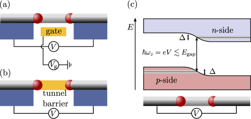
Figure 2: Possible ways to realize a fractional Josephson junction. (a) A nanowire crossing the two superconductors which is capacitively coupled to a gate at voltage $V_{\rm g}$. The gate controls the hybridization strength of the Majorana fermions at the Josephson junction. The bias voltage $V$ shifts the Fermi energies with respect to each other and leads to an a.c. Josephson effect. The panel (b) shows a similar design with less tunability since the gated part of the nanowire is replaced with a narrow layer of insulator interrupting the semiconducting nanowire. In both of these setups, the radiation frequency is bounded by the superconducting gap and thus typically is in the microwave regime. This limitation can be overcome in the design (c) which shows the band diagram of a p-n junction. The different dopings lead to a pinning of the Fermi-energy in the valence band (left) and the conduction band (right). Around the Fermi-energies a small superconducting gap is opened due to the proximity to the superconductors which leads additionally to two Majorana bound states (red spheres), on in the valence band and one in the conduction band. The junction is operated in the forward bias regime with a potential difference comparable to the band-gap $E_{\rm gap}$.

2.2 Possible realizations for fractional Josephson radiation

As the main ingredient for the present proposal, a Josephson junction where the wave function of the Majorana fermions on either side have sufficient overlap is needed. This junction then needs to be embedded in a cavity to store and amplify the radiation field. Superconducting hybrid devices are very flexible and offer many possibilities to obtain a desired physical effect. Employing this freedom, we present three different designs for realizing fractional Josephson radiation.

A possible setup involves a semiconducting nanowire covered by two conventional s-wave superconductors with a gateable junction in between, see figure 2 (a). Given the fact that the device is in its topological phase, there are four Majorana fermions formed. An external bias voltage $V$ shifts the Fermi levels of wires with respect to each other and the gate is used to control the Josephson coupling strength, i.e., the size of the Majorana wave function overlap which enters the dipole moment. It is important to note that the bias voltage is bound by the superconducting gap, $eV<|\Delta|$, as otherwise undesired quasiparticles will be generated. Given the typical size of a superconducting gap of the order of a few Kelvin, the resulting Josephson radiation will be in the microwave regime. Obviously, the gated part of the nanowire can be replaced by a narrow, insulating barrier included in the nanowire in the growth process, cf. figure 2 (b). Compared to the case (a) discussed above, one would expect a larger overlap of the wave-function in this case leading to a stronger light-matter interaction $g$ with the drawback that the parameter is not tunable any more.

Inspired by [28], there is another variant that makes use of a superconducting p-n diode, embedding a p-n diode in a semiconducting nanowire, see figure 2 (c). Doping p- and n-type carriers at the left and right side makes a p-n diode out of the wire and Majorana fermions are formed from the valence and conduction band, respectively. Recent investigations showed that the topological phase of a semiconducting nanowire persists even in presence of material imperfections (large dopant concentrations) [33]. The effect of dopants in the nanowire shifts the chemical potential towards the conduction or valence bands depending on carrier type and concentration. Typically for semiconducting nanowires there are two conduction bands and four hole bands, whereas the light-hole bands are split-off because of the boundary conditions in quasi one-dimensional wires. Light- and heavy-hole bands carry total angular momentum $J=\frac{3}{2}$ with heavy holes being characterized by $m_{J}=\pm\frac{3}{2}$. Out of the heavy hole states, Majorana fermions are formed for the hole band exactly as for the conventional electron band. Across the p-n junction the bands will bend such that the electro-chemical potential remains constant. By applying reversed bias voltage, i.e., connect the p-type side with the negative pole and the n-type side with the positive pole of a voltage source the junction acts as an insulator up to voltages of the order of the band gap $E_{\rm gap}$. The corresponding energy diagram is shown in figure 2 (c). This setup allows to increase the Josephson frequency from the superconducting gap to the band-gap $E_{\rm gap}$ of the semiconductor. For typical semiconductors with rather strong spin-orbit interaction, as for instance InAs, the band gap is of the order of $0.3\,\mathrm{eV}$ corresponding to wavelengths of around $4\,\mathrm{\mu m}$. Hence, the radiation will be emitted in the mid-infrared regime.

Similar devices have been proposed in other system involving quantum dots and a p-n junction which allows to shift the Josephson frequency into the optical frequency range [28, 29]. The proposal of [28] discusses incoherent radiation in the emission band close to half the Josephson frequency and additionally coherent emission at the Josephson frequency arising from the coherent transfer of Cooper pairs. On the other hand, the proposal of [29] leads to coherent radiation at half the Josephson frequency due to the fact that the device is embedded in a microcavity; thus, the device has been named “half-Josephson laser”. Although the optical phase of the laser is locked to the superconducting phase difference, decoherence of a half-Josephson laser is induced by spontaneous switches between different states of the quantum dot. Further elaborations have demonstrated that coherence times of emitted light from an array consisting of many emitters placed in a single cavity are exponentially long [30, 31]. The main difference of these proposals to the present work is the fact that in our case there is no need for quantum dots as the Majorana bound states are formed at the interface without additional confinement. Furthermore, the bound states are automatically aligned with the chemical potential of the superconductor and thus there is no need for (fine-)tuning of the dot parameters.

3 Model for a Josephson junction and dynamics of the radiation

3.1 Model

Even though we have advertised three different physical implementation schemes of Josephson radiation from Majorana fermions all of them can be described by a single effective model. This is because in all three setups the physical process leading to radiation is tunneling of single electrons accompanied by the emission of a photon as described by (7). Taking additionally the energy of the photons in the cavity as well as possible overlap terms between Majorana fermions on each wire section into account, we arrive at the model Hamiltonian

$$H=\frac{\varepsilon_{{\scriptscriptstyle\rm L}}}{2}\left(1-i\gamma_{1}\gamma_{2}\right)+\frac{\varepsilon_{{\scriptscriptstyle\rm R}}}{2}\left(1-i\gamma_{3}\gamma_{4}\right)+\hbar\omega a^{\dagger}a+\frac{ig}{2}\cos[\varphi(t)/2]\gamma_{2}\gamma_{3}(a+a^{\dagger})$$ (9)

which is the basis for the subsequent analysis; here, the overlap amplitudes are denoted by $\varepsilon_{{\scriptscriptstyle\rm L}}$ and $\varepsilon_{{\scriptscriptstyle\rm R}}$ for Majorana modes $\gamma_{1},\gamma_{2}$ in the left and $\gamma_{3},\gamma_{4}$ in the right section of the nanowire, respectively. These coefficients are decaying exponentially with the separation $\varepsilon_{{\scriptscriptstyle\rm L/R}}\propto e^{-L_{{\scriptscriptstyle\rm L/R}}/\xi}$, where $L_{{\scriptscriptstyle\rm L/R}}$ is the length of a particular wire section and $\xi$ is the superconducting coherence length [8]. Furthermore, it has been assumed that Majorana modes $\gamma_{1}$ and $\gamma_{4}$ are located too far away from each other such that their overlap can be neglected compared to $\varepsilon_{{\scriptscriptstyle\rm L}},\varepsilon_{{\scriptscriptstyle\rm R}}$. The applied bias voltage is taken into account by a time-dependent superconducting phase $\varphi(t)=\varphi(0)+2eVt/\hbar$. In deriving (9), we have neglected all quasiparticle excitation above the superconducting gap which leads to the requirement that $g|\langle a^{\dagger}+a\rangle|\ll|\Delta|$. Moreover, we have used the fact that we are interested in a situation where the photon frequency is $\omega\approx\omega_{J}/2$. Because of this, we neglected both the contribution from the d.c. fractional Josephson effect (8) as well as from usual Cooper pair tunneling as those contributions are off resonance. The model Hamiltonian (9) describes the dynamics of the Majorana bound states in a Josephson junction as well as dynamics of the radiation field. Note that the superconducting condensate acts as a driving force in this model. It is convenient to represent (9) in terms of a Fockspace basis consisting of states $|n\rangle\otimes|N\rangle$ where $|N\rangle$ is the state of the photon mode occupied with $N$ photons and $|n\rangle$ describing the fermionic states as introduced in (3).

Next, we assume that the voltage $eV=\hbar\omega_{{\scriptscriptstyle\rm J}}/2$ is large compared to the other characteristic energies of the system $\varepsilon_{{\scriptscriptstyle\rm L/R}},g,\Omega=\omega-\omega_{{\scriptscriptstyle\rm J}}/2$. We change via the unitary transformation $U=\exp\left(-\frac{i}{2}\omega_{{\scriptscriptstyle\rm J}}t\,a^{\dagger}a\right)$ from (9) into a rotating frame where we neglect the rapidly oscillating terms $\propto\exp(-i\omega_{J}/2)$. We then end up with the Hamiltonian

$$H_{{\scriptscriptstyle\rm RWA}}=\frac{\varepsilon_{{\scriptscriptstyle\rm L}}}{2}\left(1-i\gamma_{1}\gamma_{2}\right)+\frac{\varepsilon_{{\scriptscriptstyle\rm R}}}{2}\left(1-i\gamma_{3}\gamma_{4}\right)+\hbar\Omega b^{\dagger}b+\frac{ig}{4}\gamma_{2}\gamma_{3}(b+b^{\dagger}).$$ (10)

in the rotating wave approximation (RWA); here, we have introduced the new operators $b=e^{i\varphi(0)/2}\,a$ absorbing the superconducting phase at the initial time $t=0$.

3.2 Semiclassical approximation

As we are interested in the resonant regime of small $\Omega$, many photons will accumulate in the cavity due to the driving of the superconducting phase. If the cavity losses are small compared to the pumping rate, many photons will accumulate in the cavity and the radiation field will approach a classical state with a photon number $N=\langle b^{\dagger}b\rangle\gg 1$. We want to refer to this limit as the semiclassical limit, because the degrees of freedom of the nanowire are still treated quantum mechanically. The semiclassical approximation in (10) amounts to replacing $b$ with the complex number $\lambda=\langle b\rangle$. The Hamiltonian $H_{{\scriptscriptstyle\rm RWA}}$ becomes a $4\times 4$ matrix representing the Majorana bound states coupled to a classical field $\lambda(t)$ which is still a dynamical variable of the problem. Even though $N$ is expected to becomes large, we still want to demand $g\,|{\mathop{\rm Re}}\lambda|\ll|\Delta|$ to avoid interaction with the states above the superconducting gap $\Delta$. The equations of motion for $\lambda(t)$ can be derived from the Heisenberg equation of motion for $b$. This yields the differential equation for the classical radiation field

$$\dot{\lambda}=-\left(i\Omega+\Gamma\right)\lambda+\frac{g}{2\hbar}\langle\psi(t)|\gamma_{2}\gamma_{3}|\psi(t)\rangle,$$ (11)

where we have introduced the cavity loss rate $\Gamma$ and the (time-dependent) electronic state $|\psi(t)\rangle$. The state of the nanowire evolves according to

$$|\psi(t)\rangle=\mathcal{T}\exp\left(-\frac{i}{\hbar}\int\limits_{0}^{t}H_{{\scriptscriptstyle\rm W}}(\lambda)dt^{\prime}\right)|\psi(0)\rangle$$ (12)

with $\mathcal{T}$ the time-ordering operator and

$$H_{\scriptscriptstyle\rm W}(\lambda)=\frac{\varepsilon_{{\scriptscriptstyle\rm L}}}{2}(1-i\gamma_{1}\gamma_{2})+\frac{\varepsilon_{{\scriptscriptstyle\rm R}}}{2}(1-i\gamma_{3}\gamma_{4})+\frac{ig}{2}\gamma_{2}\gamma_{3}\,{\mathop{\rm Re}}\lambda$$ (13)

the Hamiltonian of the nanowire driven by the time-dependent field $\lambda(t)$. The two equations (11) and (12) need to be solved self-consistently. As we are interested in the long-time dynamics where the system approaches a stationary state with $\dot{\lambda}=0$, we may assume that the radiation field $\lambda$ changes slowly in time and the system adjusts adiabatically. In this regime, the system remains in its instantaneous eigenstates and $|\psi;\lambda\rangle$ which we will assume in the following.

There are four instantaneous eigenstates of $H_{\scriptscriptstyle\rm W}$ which we will denote by $|\pm,\mathcal{P};\lambda\rangle$ with $\mathcal{P}=\pm 1$ labeling the even and odd parity sectors and $\pm$ indicating whether the system is in the upper or lower state respectively. The corresponding eigenenergies are given by

$$E_{\pm,\mathcal{P}}=\frac{1}{2}\Bigl{(}\varepsilon_{{\scriptscriptstyle\rm L}}+\varepsilon_{{\scriptscriptstyle\rm R}}\pm\sqrt{g^{2}{\mathop{\rm Re}}^{2}\lambda+\delta_{\mathcal{P}}^{2}}\Bigr{)};$$ (14)

here, $\delta_{\mathcal{P}}=\varepsilon_{{\scriptscriptstyle\rm L}}+\mathcal{P}\,\varepsilon_{{\scriptscriptstyle\rm R}}$ is the size of the avoided crossing, see figure 3. The validity of the adiabatic approximation is given by $|\langle+,\mathcal{P}|\gamma_{2}\gamma_{3}|-,\mathcal{P}\rangle|\ll\frac{2}{\hbar}g\,|{\mathop{\rm Re}}\lambda|/|\frac{d}{dt}\ln({\mathop{\rm Re}}\lambda)|$ which using (11) translates to the requirement $\hbar\sqrt{\Omega^{2}+\Gamma^{2}}\ll g\,|{\mathop{\rm Re}}\lambda|$.

The initial dynamics of the radiation field before becomes close to the stationary state is highly non-adiabatic and the electronic system will switch many times between different eigenstates due to the driving of cavity field. However, we are not interested in the transient dynamics and concentrate on the stationary state of the radiation field which will turn out to be phase locked to the superconducting phase difference, see below. In the adiabatic, regime the matrix elements needed in (11) can be evaluated explicitly,

$$\langle\pm,\mathcal{P}|\gamma_{2}\gamma_{3}|\pm,\mathcal{P}\rangle=\mp i\frac{g\,{\mathop{\rm Re}}\lambda}{\sqrt{g^{2}\,{\mathop{\rm Re}}^{2}\lambda+\delta_{\mathcal{P}}^{2}}},$$ (15)

assuming that the electronic system is in the state $|\psi\rangle=|\pm,\mathcal{P}\rangle$. Plugging the matrix element into the equation of motion (11), it becomes a non-linear differential equations for the field amplitude $\lambda$. We can see that apart from the trivial stationary solution $\lambda=0$, there is for each eigenstate the second stationary solution

$$\lambda_{\pm,\mathcal{P}} =\pm\frac{1}{2}\,\sqrt{\frac{g^{2}}{4\hbar^{2}\,(\Omega^{2}+\Gamma^{2})}-4\frac{\Omega^{2}+\Gamma^{2}}{g^{2}}\,\left(\frac{\delta_{\mathcal{P}}}{\Omega}\right)^{2}}e^{i\arctan(\Gamma/\Omega)}$$ (16)

$$\approx\pm\frac{g}{4\hbar\,\sqrt{\Omega^{2}+\Gamma^{2}}}e^{i\arctan(\Gamma/\Omega)}.$$

fulfilling $\dot{\lambda}_{\pm,\mathcal{P}}=0$. The nontrivial states are stable (and correspondingly the trivial states unstable) if $4|\delta_{\mathcal{P}}|/\Omega\leq g^{2}/\hbar(\Omega^{2}+\Gamma^{2})$ which is why we have neglected $\delta_{\mathcal{P}}$ by passing from the first to the second line in (16). According to the balance between driven pumping and cavity losses, the stationary field amplitude depends on the cavity quantities $\Omega,\Gamma$ and the coupling $g$. Going back to the original non-rotating frame the stationary field configuration describes an oscillating field $\langle a\rangle=\exp[-i\omega_{{\scriptscriptstyle\rm J}}t/2-i\varphi(0)/2]\lambda_{\pm,\mathcal{P}}$ at frequency $\omega_{{\scriptscriptstyle\rm J}}/2$, i.e., half of the Josephson frequency. Regarding the phase of the radiation field $\langle a\rangle$, we see that it is locked to half of the superconducting phase difference $-\varphi(0)/2$ with an additional phase shift $\arctan(\Gamma/\Omega)$ due to the cavity. Moreover, the sign of the radiation field depends on the fact whether the system is in the upper or lower state but (almost) not on $\mathcal{P}$. This locking mechanisms protects the emitted radiation from diffusion of the phase as it is the case for conventional lasers [34]. This is a consequence of the broken $U(1)$ phase symmetry of the superconductors that is imprinted in the phase of the radiation field. we expect the coherence time of the emitted radiation to be rather long as experiments measuring the relaxation of the persistent current in superconductors have shown that the superconducting coherence lasts for years [35]. As we show in the next section, these extremely long coherence times can not be reached in realistic systems due to spontaneous switches of the electronic system as well as quasiparticle poisoning.

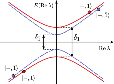
Figure 3: Spectrum of the electronic system as function of ${\mathop{\rm Re}}\lambda$. The spectrum has two distinct parity sectors indicated by solid (even) and dashed (odd) spectral-lines differing by their level splitting at zero field, $\delta_{\mathcal{P}}=\varepsilon_{{\scriptscriptstyle\rm L}}+\mathcal{P}\varepsilon_{{\scriptscriptstyle\rm R}}$. During the initial time evolution, the radiation field drives the system several times through the avoided crossing until it approaches a stationary state. There is exactly one stationary state of the radiation field, indicated by the dots, associated with each eigenstate of the electronic system.

4 Coherence of the radiation

Switches of the electronic state of the wire are caused by two mechanisms, emission of off-resonant photons and quasiparticle poisoning, that are present even if the stationary state has been reached. Whenever a spontaneous switching event happens, the cavity field will be driven out of its stationary state and eventually will approach another one. Here, we will assume that switches happen instantaneously on the time-scale $\Gamma^{-1}$ of the cavity. While the system approaches another stable amplitude the time evolution may get non-adiabatic again including many other switching processes as described in Sec. 3.1. As noted above, in case the switching process changes the electronic system from the upper to the lower branch (or the other way round), it is accompanied with a change of $\pi$ of the phase of the radiation field. We will discuss two mechanism which lead to decoherence: The first process we will discuss conserves the total parity $\mathcal{P}$. By emitting a non-resonant photon that carries the energy of the level splitting $\hbar\tilde{\omega}\simeq g\,|{\mathop{\rm Re}}\lambda|$, a transition between those upper and lower states at fixed parity is possible. The transition rate for such a process can be evaluated by Fermi’s golden rule. Using the fact that the density of state of the photons in the cavity is Lorentzian, we obtain the approximate transition rate [29]

$$\Gamma_{{\scriptscriptstyle\rm F}}=\frac{\Gamma}{8}\left(\frac{\delta_{\mathcal{P}}}{g\,{\mathop{\rm Re}}^{2}\lambda}\right)^{2},$$ (17)

where we have assumed that the photon frequency is far detuned, $\tilde{\omega}\gg\Gamma,\Omega$. Given the fact that $\delta_{\mathcal{P}}$ depends exponentially on the separation of the Majorana fermions, we expect that $\Gamma_{\scriptscriptstyle\rm F}$ will most likely be not the dominating process generating decoherence but rather the fact that superconducting devices suffer from quasi-particle poisoning. As soon as an extra quasi-particles tunnels on one of the bulk superconductors the parity of the device is changed. Additionally, also the upper state might be transformed into the lower state as the quasiparticle changes $\mathcal{P}_{{\scriptscriptstyle\rm L}}$ or $\mathcal{P}_{{\scriptscriptstyle\rm R}}$ which do not commute with the Hamiltonian $H_{\scriptscriptstyle\rm W}$. For concreteness, we assume that a quasiparticle tunneling switches the state $|+,\mathcal{P}\rangle$ to the states $|\pm,\bar{\mathcal{P}}\rangle$ with equal probability. Measurements of transmon-type charge qubits have shown that quasi-particle tunneling appears to happen on rather long time scales in the range from microseconds up to milliseconds [36]. In the following quasi-particle tunneling will be modeled simply by a $\Gamma_{{\scriptscriptstyle\rm QP}}$. On top of these spontaneous switches, there are coherent Rabi oscillations with frequency $g\,|{\mathop{\rm Re}}\lambda|$ taking place because of the influence of counter-rotating terms that have been neglected in the RWA. See B for details.

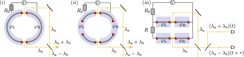
Figure 4: Three different designs for small networks with two Josephson junctions. In (i), a single semiconducting (circular) nanowire is lying on top two bulk superconductors realizing a d.c.-SQUID geometry interrupted by two Josephson junctions. In the setup (ii), the two fractional Josephson junctions in the d.c.-SQUID are formed by two distinct nanowires such that there are eight Majorana zero modes in total. In (iii), the two fractional Josephson junctions are two independent setups of figure 1 biased at the same voltage $V$. Each Josephson junction is surrounded by a microcavity which emits coherent radiation indicated by beams of radiation $\lambda_{\rm a}$ and $\lambda_{\rm b}$. These radiation fields are subsequently lead to interfere by a semitransparent mirror (dashed line). In the main text, we compare the expected coherence of the radiation emitted in these different setups with each other.

4.1 Autocorrelations and partial coherence

Including the action of both switching mechanisms, the question arises on what time-scale the Josephson radiation remains coherent. In this section we want to address the question of autocorrelations of the radiation emitted by a single Josephson junction, whereas the correlations between different sources are discussed in the next section.

The correlations of the radiation field can be determined from a master equation treatment of the switching processes. The main task of the master equation is to evaluate the vector $\bm{p}(t)$ whose components are the probabilities $p_{\alpha}(t)$ for finding the system in a particular state $\alpha\in|\pm,\mathcal{P}\rangle$ at time $t$ given some initial state $\bm{p}(0)$. The master equation describing the switching events then reads

$$\dot{\bm{p}}=\left[-(\Gamma_{{\scriptscriptstyle\rm F}}+\Gamma_{{\scriptscriptstyle\rm QP}})\leavevmode\hbox{\small 1\normalsize\kern-3.30002pt1}_{4}+\Gamma_{{\scriptscriptstyle\rm F}}\sigma_{1}+\frac{\Gamma_{{\scriptscriptstyle\rm QP}}}{2}(\leavevmode\hbox{\small 1\normalsize\kern-3.30002pt1}_{2}+\sigma_{1})\tau_{1}\right]\bm{p}$$ (18)

where $\sigma_{j}$ ($\{\tau_{j}\}$) are Pauli-matrices acting on the first (second) label of $|\pm,\mathcal{P}\rangle$. The time evolution of the radiation field is thus given by

$$\langle\Lambda(t)\rangle=\sum_{\alpha}e^{-i\varphi(t)/2}\lambda_{\alpha}\,p_{\alpha}(t)$$ (19)

where the angular brackets indicate the ensemble average and we have assumed that the radiation field is always in its stationary state $\lambda_{\alpha}$ which corresponds to demanding that $\Gamma\gg\Gamma_{\scriptscriptstyle\rm QP},\Gamma_{\scriptscriptstyle\rm F}$. In general, correlations can be expressed in terms of the normalized first-order correlation function

$$g^{(1)}(\tau)=\frac{\langle\Lambda^{*}(t)\Lambda(t+\tau)\rangle}{\langle|\Lambda|^{2}\rangle}.$$ (20)

correlating the signal $\lambda(t)$ with itself after a time $\tau$. Without the switching processes discussed before, the autocorrelation function is one indicating coherence with an infinite coherence time. The situation changes when spontaneous switches are taken into account. Then the relative phase factors of $\lambda$ changes randomly by $\pi$ resulting in a finite coherence time.

Autocorrelations of each beam can be measured by performing a Hanbury Brown-Twiss experiment measuring intensity correlations of the radiation field at the different times $t$ and $t+\tau$. In fact, the first order autocorrelation function and with that its coherence time can be extracted from the normalized second order correlation function via

$$g^{(2)}=\frac{\langle\Lambda^{*}(t)\Lambda^{*}(t+\tau)\Lambda(t+\tau)\Lambda(t)\rangle}{\langle|\Lambda|^{2}\rangle^{2}}=1+|g^{(1)}(\tau)|^{2}$$ (21)

where the last identity is valid for a classical radiation field as we are considering [37]. The solution of the master equation for $\bm{p}$ yields in the steady state the first-order correlation function

$$g^{(1)}(\tau)=\exp\left(-\frac{i}{2}\omega_{{\scriptscriptstyle\rm J}}\tau-\frac{\tau}{\tau_{\rm c}}\right)$$ (22)

where $\tau_{\rm c}=(2\Gamma_{{\scriptscriptstyle\rm F}}+\Gamma_{{\scriptscriptstyle\rm QP}})^{-1}$ is the coherence time. The reason for the factor two of $\Gamma_{\scriptscriptstyle\rm F}$ compared to $\Gamma_{\scriptscriptstyle\rm QP}$ is the fact that the former process leads every time to a switch of the upper to the lower state whereas for the former process this happens only with a probability of 50%.

Another effect which leads to decoherence are thermal fluctuations of the bias voltage. Since there is a finite resistance $R_{0}$ associated to the circuit that connects the ideal voltage source with the Josephson junction, cf. figure 4, there is a Johnson-Nyquist noise characterized by $\langle\langle V(t)V(t+\tau)\rangle\rangle=2R_{0}k_{{\scriptscriptstyle\rm B}}T\delta(\tau)$ at any finite temperature $T$. As the first-order correlation function is proportional to the complex phase factor $e^{i[\varphi(t)-\varphi(t+\tau)]/2}$ and thus depends on $V(t)$, the thermal noise leads to decoherence. Using the fact that the thermal noise is Gaussian, the expectation value of the complex phase factor assumes the form

$$\langle e^{i[\phi(t)-\phi(t+\tau)]/2}\rangle=e^{-i\omega_{\scriptscriptstyle\rm J}\tau/2}e^{-\langle\langle[\varphi(t)-\varphi(t+\tau)]^{2}\rangle\rangle/8}=\exp\left(-\frac{i}{2}\omega_{\scriptscriptstyle\rm J}\tau-\frac{e^{2}R_{0}}{\hbar^{2}}k_{{\scriptscriptstyle\rm B}}T\tau\right).$$ (23)

Consequently, the normalized auto-correlation function is given by

$$g^{(1)}(\tau)=\exp\left[-\frac{i}{2}\omega_{\scriptscriptstyle\rm J}\tau-\left(\tau_{\rm c}^{-1}+\frac{e^{2}R_{0}}{\hbar^{2}}k_{{\scriptscriptstyle\rm B}}T\right)\tau\right]$$ (24)

with a reduced coherence time due to the finite resistance $R_{0}$.

4.2 Correlations of different sources

So far, we have discussed the dynamics and stationary properties of the emitted Josephson radiation of a single junction. In this section, we want to expand the setup and take possible coherence between different emitters into account. Due to the phase locking, we expect that the radiation fields are ideally perfectly correlated with each other [28]. Hence, it should be possible to observe correlations between two radiation fields even if these junctions are spatially-separated from each other.

Here, we want to determine the correlation between different radiation sources for the three setups illustrated in figure 4. We will label the properties associated with two radiation sources by a and b. The coherence will show up in the second-order correlation function

$$g_{\rm ab}^{(2)}(\tau)=\frac{\langle\Lambda^{*}_{\rm a}(t)\Lambda^{*}_{\rm b}(t+\tau)\Lambda_{\rm b}(t)\Lambda_{\rm a}(t+\tau)\rangle}{\langle|\Lambda_{\rm a}|^{2}\rangle\langle|\Lambda_{\rm b}|^{2}\rangle}$$ (25)

measuring correlations between two radiation fields $\lambda_{\rm a}$, $\lambda_{\rm b}$. The function $g_{\rm ab}^{(2)}(\tau)$ is part of the intensity correlators $\langle|\Lambda_{\rm a}(t)\pm\Lambda_{\rm b}(t)|^{2}\,|\Lambda_{\rm a}(t+\tau)\pm\Lambda_{\rm b}(t+\tau)|^{2}\rangle$ and thus can be measured by correlating the intensities after the beamsplitters, see figure 4 (iii).

The first setup, we analyze is shown in figure 4 (i). There is a single circular nanowire placed on a superconducting ring interrupted by two Josephson junctions (d.c.-SQUID geometry). Each of these junctions implements a source as discussed above. For simplicity, we assume both junctions to be equal, i.e., $g_{\rm a}=g_{\rm b}=g$, $\Omega_{\rm a}=\Omega_{\rm b}=\Omega$, and $\Gamma_{\rm a}=\Gamma_{\rm b}=\Gamma$. In total there will be four Majorana fermions in the system and the equations of motion assume the form

$$\dot{\lambda}_{\rm a} =-(i\Omega+\Gamma)\lambda_{\rm a}\pm i\frac{g^{2}}{4\hbar}\,\frac{{\mathop{\rm Re}}(\lambda_{\rm a}-\mathcal{P}\lambda_{\rm b})}{\sqrt{\delta_{\mathcal{P}}^{2}+g^{2}{\mathop{\rm Re}}^{2}(\lambda_{\rm a}-\mathcal{P}\lambda_{\rm b})}},$$

$$\dot{\lambda}_{\rm b} =-(i\Omega+\Gamma)\lambda_{\rm b}\pm i\frac{g^{2}}{4\hbar}\,\frac{{\mathop{\rm Re}}(\lambda_{\rm b}-\mathcal{P}\lambda_{\rm a})}{\sqrt{\delta_{\mathcal{P}}^{2}+g^{2}{\mathop{\rm Re}}^{2}(\lambda_{\rm a}-\mathcal{P}\lambda_{\rm b})}},$$ (26)

with $\mathcal{P}$ the total fermion parity of the system, as before. The stationary solutions are given by (16) with the additional constraint $\lambda_{\rm b}=-\mathcal{P}\lambda_{\rm a}$ which correlates both field amplitudes $\lambda_{\rm a}$ and $\lambda_{\rm b}$ by the parity constraint. Hence the d.c.-SQUID geometry exhibits a strong correlation between different stationary fields for arbitrary spatial-separation. In particular, the constraint implies that the relative phase between $\lambda_{\rm a}$ and $\lambda_{\rm b}$ can only be changed by changing the total fermion parity of the system, i.e., quasi-particle poisoning. Indeed, we obtain the result

$$g_{\rm ab}^{(2)}(\tau)=\exp(-2\Gamma_{{\scriptscriptstyle\rm QP}}\tau).$$ (27)

for the case (i). Note that this result is independent of the resistance $R_{0}$ of the voltage source.

The case (i) shows very robust correlations but we expect it to be rather challenging to realize experimentally as a circular nanowire is required. Therefore, we want to analyze the situation where the two emitters are formed by two different nanowires, see figure 4 (ii). In contrast to the last case, there are in total eight Majorana fermions involved in this case—four on each nanowire. As a result, there is no parity constraint relating the phase of the field of one emitter to the field of the other emitter in the stationary state. Instead, the Hamiltonian of the wires separates into two parts $H_{\rm a}+H_{\rm b}$ with only the common superconducting phase providing correlations. Thus, the stationary state of the radiation fields in the rotating frame are individually given by (16). In the laboratory frame, the states evolve according to $e^{-i\varphi(t)/2}\lambda_{\rm a/b}$ with the common superconducting phase-difference $\varphi(t)$ which is expected to lead to partial coherence of the sources. Indeed, calculating the correlation function for this case, we obtain

$$g_{\rm ab}^{(2)}(\tau)=\exp[-2(2\Gamma_{{\scriptscriptstyle\rm F}}+\Gamma_{{\scriptscriptstyle\rm QP}})\tau]$$ (28)

which is decaying with the typical time scale $\tau_{\rm c}$ of the spontaneous switching events. As above, the result is independent of the resistance $R_{0}$.

The last case (iii) differs from (ii) by the fact that the radiation-emitting junctions do not share common superconductors but only a common voltage source. In this case, the phase-difference $\varphi_{\rm a}$ will differ from $\varphi_{\rm b}$ which leads to decoherence of the two radiation fields evolving according to $e^{-i\varphi_{\rm a/b}(t)/2}\lambda_{\rm a/b}$ in the laboratory frame. In fact, the diffusion of the difference $\varphi_{\rm a}-\varphi_{\rm b}$ will be governed by the resistance $R$, cf. figure 4 (iii). Because of that the second-order correlation function

$$g_{\rm ab}^{(2)}(\tau)=\exp\left[-2(2\Gamma_{{\scriptscriptstyle\rm F}}+\Gamma_{{\scriptscriptstyle\rm QP}})\tau-\frac{e^{2}R}{\hbar^{2}}k_{{\scriptscriptstyle\rm B}}T\tau\right].$$ (29)

shows an additional decay compared to (28).

5 Conclusions

In this work, we have analyzed the possibility of coupling Majorana fermions to electromagnetic fields. We have shown that partially coherent Josephson radiation is emitted at half of the Josephson frequency. The coherence of the radiation is limited due to rare spontaneous switches of the relative phase flipping randomly between values $0,\pi$. Due to the coupling of the Majorana zero modes to the superconductor, there are only two phases differences allowed. It leads to a fixed phase of the radiation field different from conventional lasers where the optical phase is slowly diffusing [34]. Even though the phases are in principle locked, decoherence of the radiation is induced by spontaneous switches as well as by frequency fluctuations. We have analyzed the correlation between two emitters which are spatially-separated but share the same superconductors. We have discussed the effect of the fermionic parity constraint in a d.c.-SQUID geometry as well as the pinning of the Josephson frequency in terms of a second order correlator and suggested a possible way to experimentally obtain this information. The interaction of Majorana fermions with radiation could potentially be used for addressing and manipulating Majorana states beyond driving since the radiation field carries all the information about the state of the nanowire.

Appendix A Dipole operator for Majorana fermions

The matrix elements of the electric dipole operator in the Majorana ground state manifold are solutions of the Bogoliubov-de Gennes equation, $\mathcal{H}_{\rm BdG}\,\xi_{n}(\bm{r})=E_{n}\,\xi_{n}(\bm{r})$ with the Nambu-spinor $\xi_{n}(\bm{r})=(u_{n}(\bm{r}),v_{n}(\bm{r}))^{\rm t}$ [35]. From these solutions $\{\xi_{n}\}$ the Bogoliubov quasiparticle operators can be obtained obtained via

$$\beta_{n}=\int[u^{*}_{E_{n}}(\bm{r})\psi(\bm{r})+v^{*}_{E_{n}}(\bm{r})\psi^{\dagger}(\bm{r})]\,d^{3}r,$$ (30)

with $\beta_{n},\beta_{n}^{\dagger}$ obeying the canonical anticommutation relations, $\{\beta_{m},\beta_{n}^{\dagger}\}=\delta_{mn}$. Every BdG-Hamiltonian carries a build-in particle hole symmetry which is represented by an operator $\Xi=\tau_{x}\mathcal{K}$ that is anti commuting with the BdG Hamiltonian $\{\mathcal{H}_{\rm BdG},\Xi\}=0$. Here $\tau_{x}$ denotes the Pauli $x$ matrix in Nambu space and $\mathcal{K}$ is the complex conjugation. The operator $\Xi$ maps a solution of the BdG equation to its particle-hole reversed partner $\xi_{-n}=\Xi\,\xi_{n}$, which is again a solution of the BdG equation having eigenvalue $-E_{n}$. In particular, the eigenspace related to solutions at zero energy $\{\xi_{\mu}|\;\mathcal{H}_{\rm BdG}\xi_{\mu}=0\}$ needs to contain an even number of solutions. Given a zero energy solution $\xi_{\mu}$, one can choose a different basis which is the eigenbasis of the particle-hole operator via $\zeta_{\mu}=\xi_{\mu}+\Xi\xi$ and $\bar{\zeta}_{\mu}=i(\Xi\xi_{\mu}-\xi_{\mu})$. The new spinors are invariant with respect to electron-hole inversion $\Xi\zeta_{\mu}=\zeta_{\mu}$ which constitutes a condition for Majorana fermions. The new spinors are given by $\zeta_{\mu}=(w_{\mu},w_{\mu}^{*}),\bar{\zeta}_{\mu}=(\bar{w}_{\mu},\bar{w}^{*}_{\mu})$ with components $w_{\mu}(\bm{r})=u_{\mu}(\bm{r})+v_{\mu}^{\ast}(\bm{r})$ and $\bar{w}=iu_{\mu}(\bm{r})-iv_{\mu}^{*}(\bm{r})$. In the language of second quantization one gets a new set of Hermitian operators

$$\gamma_{\mu} =\beta^{\dagger}_{\mu}+\beta^{{\vphantom{\dagger}}}_{\mu},\qquad\bar{\gamma}_{\mu}=i(\beta^{\dagger}_{\mu}-\beta^{{\vphantom{\dagger}}}_{\mu}),$$ (31)

fulfilling the algebra of Majorana bound states $\{\gamma_{\mu},\gamma_{\nu}\}=2\delta_{\mu\nu}$. The existence of these zero energy modes is guaranteed by the topological structure of the BdG Hamiltonian $\mathcal{H}_{\rm BdG}(k)$ in presence of (effective) p-wave pairing potentials. Using the reversed Bogoliubov transformation (30),

$$\psi(\bm{r})=\sum_{m}[u_{m}(\bm{r})\beta_{m}+v^{*}_{m}(\bm{r})\beta_{m}^{\dagger}],$$ (32)

it is a straightforward task to represent a second quantized operator in terms of Bogoliubov quasi-particles. By restricting the general expression on the subspace of zero energy solutions only, any observable $O$ can be expressed in terms of Majorana operators as follows

$$O =\int\psi^{\dagger}(\bm{r}^{\prime})O(\bm{r}^{\prime},\bm{r})\psi(\bm{r}^{\prime})\,d^{3}r^{\prime}d^{3}r$$ (33)

$$=\frac{1}{4}\sum_{\mu,\nu}\left[\int w^{\ast}_{\mu}(\bm{r}^{\prime})O(\bm{r}^{\prime},\bm{r})w_{\nu}(\bm{r})\,d^{3}r^{\prime}d^{3}r\right]\gamma_{\mu}\gamma_{\nu}=\frac{i}{4}\sum_{\mu,\nu}\mathcal{O}_{\mu\nu}\gamma_{\mu}\gamma_{\nu},$$

where the sum runs over all Majorana fermions $\gamma_{\mu},\bar{\gamma}_{\mu}$ in the last two lines. As the coefficient in front of the Majorana operators is a Hermitian scalar product with respect to the Majorana wave functions $w_{\mu}(\bm{r}^{\prime})$ and $w_{\nu}(\bm{r})$. This matrix element can only have a finite value where two Majorana wave functions have a considerable overlap. Because the Majorana wave function is spatially localized at the ends of the nanowire finite matrix elements can only appear at Josephson junctions where two Majorana modes are close together. Note, that the matrix elements are be antisymmetric, $\mathcal{O}_{\mu\nu}=-\mathcal{O}_{\nu\mu}$, in the Majorana basis.

Matrix elements between Majorana operators located at two different sides of a Josephson junction acquire a non-trivial phase dependency. This can be derived by performing a gauge transformation of the BdG Hamiltonian. From general principles, it is clear that a non-trivial phase difference $\varphi\neq 0$ cannot be gauged away. Therefore all matrix elements connecting degrees of freedom on both sides of the Josephson junction acquire phase factors $e^{\pm i\varphi/2}$ whereas all others become independent of the superconducting phases. In particular, if the operator $O$ connects two Majorana fermions $\gamma_{\mu},\gamma_{\nu}$ across a Josephson junction we obtain the representation

$$O =\frac{i}{4}e^{i\varphi/2}\mathcal{O}_{\mu\nu}\gamma_{\mu}\gamma_{\nu}+\frac{i}{4}e^{-i\varphi/2}\mathcal{O}_{\nu\mu}\gamma_{\nu}\gamma_{\mu}=\frac{i}{2}\cos(\varphi/2)\mathcal{O}_{\mu\nu}\gamma_{\mu}\gamma_{\nu},$$ (34)

where the dependence on the superconducting phase keeps track of the charge that is transported across the junction. Accordingly, for the electrical dipole operator we get the following representation in terms of Majorana operators

$$\bm{d}=-e\int\psi^{\dagger}(\bm{r})\,\bm{r}\psi(\bm{r})\,d^{3}r=\frac{i}{2}\sum_{\mu<\nu}\cos(\varphi/2)\bm{d}_{\mu\nu}\gamma_{\mu}\gamma_{\nu}$$ (35)

where the matrix elements of the dipole operator are given by

$$\bm{d}_{\mu\nu}=-e\int\bm{r}\,w^{*}_{\mu}(\bm{r})w_{\nu}(\bm{r})\,d^{3}r.$$ (36)

Note again that these quantities are only non-zero if the Majorana wave functions have some overlap.

Appendix B Influence of counter-rotating terms

In order to study the effect of the counter-rotating terms that have been neglected in (10) the non-rotating stationary solutions are put into the original Hamiltonian (9) substituting operator $a$ by $\exp(-i\varphi(t)/2)\lambda$. The resulting Hamiltonian is given by

$$H =\frac{\varepsilon_{{\scriptscriptstyle\rm L}}+\varepsilon_{{\scriptscriptstyle\rm R}}}{2}\leavevmode\hbox{\small 1\normalsize\kern-3.30002pt1}_{2}+\frac{\delta_{\mathcal{P}}}{2}\sigma_{3}-\frac{g|\lambda|}{2}\cos(\chi)\sigma_{1}+\frac{g|\lambda|}{2}\cos(\omega_{{\scriptscriptstyle\rm J}}t+\varphi(0)-\chi)\sigma_{1},$$ (37)

where the last term represents fast oscillating counter-rotating terms, that have been neglected while going from (9) to (10). Furthermore, $\chi=\arctan(\Gamma/\Omega)$ is the phase shift due to the cavity and $\sigma_{1}=i\gamma_{2}\gamma_{3},\sigma_{3}=-i\gamma_{1}\gamma_{2}$ are Pauli matrices. This is a time-dependent problem with driving frequency $\omega_{{\scriptscriptstyle\rm J}}$. After interchanging $\sigma_{1}$ and $\sigma_{3}$, we make the ansatz [38]

$$|\phi\rangle=\exp\left(i\frac{g|\lambda|}{2\hbar}\int\limits_{0}^{t}\cos(\omega_{{\scriptscriptstyle\rm J}}t+\varphi(0)-\chi)dt\,\sigma_{3}\right)|\tilde{\phi}\rangle$$ (38)

for the wave function $|\phi\rangle$. This leads to the Schrödinger equation for $|\tilde{\phi}\rangle$

$$i\hbar\partial_{t}\left(\begin{array}[]{c}\tilde{\phi}_{1}\\ \tilde{\phi}_{2}\end{array}\right)=\frac{1}{2}\left(\begin{array}[]{cc}-g|\lambda|\cos{\chi}&e^{iA(t)}\delta_{\mathcal{P}}\\ e^{-iA(t)}\delta_{\mathcal{P}}&g|\lambda|\cos{\chi}\end{array}\right)\left(\begin{array}[]{c}\tilde{\phi}_{1}\\ \tilde{\phi}_{2}\end{array}\right)$$ (39)

with the time-dependent expression $A(t)=\frac{g|\lambda|}{2\hbar\omega_{{\scriptscriptstyle\rm J}}}[\sin(\omega_{{\scriptscriptstyle\rm J}}t+\varphi(0)-\chi)-\sin(\varphi(0)-\chi)]$. Since the driving frequency is much larger than the largest energy scale in (39), $g|\lambda|\ll\hbar\omega_{{\scriptscriptstyle\rm J}}$ it is reasonable to perform a time average over one period $T=\omega_{{\scriptscriptstyle\rm J}}/2\pi$. From the resulting time-averaged Schrödinger equation the probability for a state inversion flip is obtained to

$$P_{+\rightarrow-}(t) =|\langle\phi_{-}|\phi_{+}(t)\rangle|^{2}\approx\left(\frac{\delta_{\mathcal{P}}}{g\,{\mathop{\rm Re}}\lambda}\right)^{2}\sin^{2}\left(\frac{g\,|{\mathop{\rm Re}}\lambda|}{2\hbar}\,t\right).$$ (40)

The probability to flip from the upper to the lower state is apparently oscillating in a coherent manner with period $4\pi\hbar/g\,|{\mathop{\rm Re}}\lambda|\ll\Gamma^{-1}$.

References

References

- [1] Josephson B D 1962 Phys. Lett. 1 251
- [2] Lee P A and Scully M O 1971 Phys. Rev. B 3 769
- [3] Yanson I K, Svistuno V M and Dmitrenko I M 1965 JETP Lett. 21 650
- [4] Langenberg D N, Scalapino D J, Taylor B N and Eck R E 1965 Phys. Rev. Lett. 15 294
- [5] De Franceschi S, Kouwenhoven L, Schönenberger C and Wernsdorfer W 2010 Nature Nanotech. 5 703
- [6] Brouwer P 2012 Science 336 989
- [7] Franz M 2013 Nature Nanotech. 8 149
- [8] Kitaev A Y 2001 Phys.-Usp. 44 131
- [9] Alicea J 2012 Rep. Prog. Phys. 75 076501
- [10] Beenakker C 2013 Annu. Rev. Cond. Mat. Phys. 4 113
- [11] Leijnse M and Flensberg K 2012 Semicond. Sci. Tech. 27 124003
- [12] Oreg Y, Refael G and von Oppen F 2010 Phys. Rev. Lett. 105 177002
- [13] Lutchyn R M, Sau J D and Das Sarma S 2010 Phys. Rev. Lett. 105 077001
- [14] Mourik V, Zuo K, Frolov S M, Plissard S R, Bakkers E P A M and Kouwenhoven L P 2012 Science 336 1003
- [15] Rokhinson L P, Liu X and Furdyna J K 2012 Nature Phys. 8 795
- [16] Das A, Ronen Y, Most Y, Oreg Y, Heiblum M and Shtrikman H 2012 Nature Phys. 8 887
- [17] Deng M T, Yu C L, Huang G Y, Larsson M, Caroff P and Xu H Q 2012 Nano Lett. 12 6414
- [18] Fu L 2010 Phys. Rev. Lett. 104 056402
- [19] Fu L and Kane C L 2009 Phys. Rev. B 79 161408
- [20] Kwon H J, Sengupta K and Yakovenko V M 2004 Eur. Phys. J. B 37 349
- [21] Pikulin D I and Nazarov Yu V 2012 Phys. Rev. B 86 140504
- [22] San-Jose P, Prada E and Aguado R 2012 Phys. Rev. Lett. 108 257001
- [23] Houzet M, Meyer J S, Badiane D M and Glazman L I 2013 Phys. Rev. Lett. 111 046401
- [24] Domínguez F, Hassler F and Platero G 2012 Phys. Rev. B 86 140503
- [25] Virtanen P and Recher P arXiv:1303.2353
- [26] Schmidt T L, Nunnenkamp A and Bruder C 2013 New J. Phys. 15 025043
- [27] Ginossar E and Grosfeld E 2013 arXiv:1307.1159
- [28] Recher P, Nazarov Yu V and Kouwenhoven L P 2010 Phys. Rev. Lett. 104 156802
- [29] Godschalk F, Hassler F and Nazarov Yu V 2011 Phys. Rev. Lett. 107 073901
- [30] Godschalk F and Nazarov Yu V 2013 Phys. Rev. B 87 094511
- [31] Godschalk F and Nazarov Yu V 2013 Europhys. Lett. 103 28005
- [32] van Heck B, Hassler F, Akhmerov A R and Beenakker C W J 2011 Phys. Rev. B 84 180502(R)
- [33] Adagideli I, Wimmer M and Teker A 2013 arXiv:1302.2612
- [34] Scully M O and Lamb W E 1967 Phys. Rev. 159 208
- [35] Tinkham M 1996 Introduction to Superconductivity 2nd ed (New York: McGraw-Hill)
- [36] Riste D, Bultink C C, Tiggelman M J, Schouten R N, Lehnert K W and DiCarlo L 2013 Nature Commun. 4 1913
- [37] Loudon R 1973 The quantum theory of light (London: Oxford University Press)
- [38] Nazarov Yu and Blanter Ya 2009 Quantum Transport (Cambridge University Press, New York)