Decompositions of Triangle-Dense Graphs

Abstract

High triangle density — the graph property stating that a constant fraction of two-hop paths belong to a triangle — is a common signature of social networks. This paper studies triangle-dense graphs from a structural perspective. We prove constructively that significant portions of a triangle-dense graph are contained in a disjoint union of dense, radius $2$ subgraphs. This result quantifies the extent to which triangle-dense graphs resemble unions of cliques. We also show that our algorithm recovers planted clusterings in approximation-stable $k$-median instances.

1 Introduction

Can the special structure possessed by social networks be exploited algorithmically? Answering this question requires a formal definition of “social network structure.” Extensive work on this topic has generated countless proposals but little consensus (see e.g. [CF06]). The most oft-mentioned (and arguably most validated) statistical properties of social networks include heavy-tailed degree distributions [BA99, BKM⁺00, FFF99], a high density of triangles [WS98, SCW⁺10, UKBM11] and other dense subgraphs or “communities” [For10, GN02, New03, New06, LLDM08], and low diameter and the small world property [Kle00a, Kle00b, Kle02, New01].

Much of the recent mathematical work on social networks has focused on the important goal of developing generative models that produce random networks with many of the above statistical properties. Well-known examples of such models include preferential attachment [BA99] and related copying models [KRR⁺00], Kronecker graphs [CZF04, LCK⁺10], and the Chung-Lu random graph model [CL02a, CL02b]. A generative model articulates a hypothesis about what “real-world” social networks look like, and is directly useful for generating synthetic data. Once a particular generative model of social networks is adopted, a natural goal is to design algorithms tailored to perform well on the instances generated by the model. It can also be used as a proxy to study the effect of random processes (like edge deletions) on a network. Examples of such results include [AJB00, LAS⁺08, MS10].

This paper pursues a different approach. In lieu of adopting a particular generative model for social networks, we ask:

• Is there a combinatorial assumption weak enough to hold in every “reasonable” model of social networks, yet strong enough to permit useful structural and algorithmic results?

That is, we seek algorithms that offer non-trivial guarantees for every reasonable model of social networks, including those yet to be devised.

Triangle-Dense Graphs

We initiate the algorithmic study of triangle-dense graphs. Let a wedge be a two-hop path in an undirected graph.

Definition 1 (Triangle-Dense Graph).

The triangle density of an undirected graph $G=(V,E)$ is $\tau(G):=3t(G)/w(G)$, where $t(G)$ is the number of triangles in $G$ and $w(G)$ is the number of wedges in $G$ (conventionally, $\tau(G)=0$ if $w(G)=0$). The class of $\epsilon$-triangle dense graphs consists of the graphs $G$ with $\tau(G)\geq\epsilon$.

Since every triangle of a graph contains 3 wedges, and no two triangles share a wedge, the triangle density of a graph is between 0 and 1. We use the informal term “triangle dense graphs” to mean graphs with constant triangle density. In the social sciences, triangle density is usually called the transitivity of a graph [WF94]. We use the term triangle density because “transitivity” already has strong connotations in graph theory.

As an example, the triangle density of a graph is 1 if and only if it is the union of cliques. The triangle density of an Erdös-Renyi graph, drawn from $G(n,p)$, is concentrated around $p$. Thus, only very dense Erdös-Renyi graphs have constant triangle density. Social networks are generally sparse and yet have remarkably high triangle density; the Facebook graph, for instance, has triangle density $0.16$ [UKBM11]. High triangle density is perhaps the least controversial signature of social networks (see related work below).

The class of $\epsilon$-triangle dense graphs becomes quite diverse as soon as $\epsilon$ is bounded below 1. For example, the complete tripartite graph is triangle dense. Every graph obtained from a bounded-degree graph by replacing each vertex with a triangle is triangle dense. Adding a clique on $n^{1/3}$ vertices to a bounded-degree $n$-vertex graph produces a triangle-dense graph. We give a litany of examples in §4. Can there be interesting structural or algorithmic results for this rich class of graphs?

Our Results: A Decomposition Theorem

Our main decomposition theorem quantifies the extent to which a triangle-dense graph resembles a union of cliques. The next definition gives our notion of an “approximate union of cliques.” We use $G|_{S}$ to denote the subgraph of a graph $G$ induced by a subset $S$ of vertices. Also, the edge density of a graph $G=(V,E)$ is $|E|/\binom{|V|}{2}$.

Definition 2 (Tightly Knit Family).

Let $\rho>0$. A collection $V_{1},V_{2},\ldots,V_{k}$ of disjoint sets of vertices of a graph $G=(V,E)$ forms a $\rho$-tightly-knit family if:

• Each subgraph $G|_{V_{i}}$ has both edge density and triangle density at least $\rho$.

• Each subgraph $G|_{V_{i}}$ has radius at most $2$.

When $\rho$ is a constant, we often refer simply to a tightly-knit family. Every “cluster” of a tightly-knit family is dense in edges and in triangles. In the context of social networks, an abundance of triangles is generally associated with meaningful social structure.

Our main decomposition theorem states that every triangle-dense graph contains a tightly-knit family that captures a constant fraction of the graph’s triangles.

Result 1 (Main Decomposition Theorem).

There exists a polynomial $f$ such that for every $\epsilon$-triangle dense graph $G$, there exists an $f(\epsilon)$-tightly-knit family that contains an $f(\epsilon)$ fraction of the triangles of $G$.

We emphasize that Result 1 requires only that the input graph $G$ is triangle dense — beyond this property, it could be sparse or dense, low- or high-diameter, and possess an arbitrary degree distribution. Graphs that are not triangle dense, such as sparse Erdös-Renyi random graphs, do not generally admit non-trivial tightly-knit families (even if the triangle density requirement for each cluster is dropped).

Our proof of Result 1 is constructive. Using suitable data structures, the resulting algorithm can be implemented to run in time proportional to the number of wedges of the graph; a detailed implementation is available from the authors. This running time is reasonable for many social networks. Our preliminary implementation of the algorithm requires a few minutes on a commodity laptop to decompose networks with millions of edges.

Note that Result 1 is non-trivial only because we require that the tightly-knit family preserve the “interesting social information” of the original graph, in the form of the graph’s triangles. Extracting a single low-diameter cluster rich in edges and triangles is easy — large triangle density implies that typical vertex neighborhoods have these properties. But extracting such a cluster carelessly can do more harm than good, destroying many triangles that only partially intersect the cluster. Our proof of Result 1 shows how to repeatedly extract low-diameter dense clusters while preserving at least a constant fraction of the triangles of the original graph.

A triangle-dense graph need not contain a tightly-knit family that contains a constant fraction of the graph’s edges; see the examples in §4. The culprit is that triangle density is a “global” condition and does not guarantee good local triangle density everywhere, allowing room for a large number of edges that are intuitively spurious. Under the stronger condition of constant local triangle density, however, we can compute a tightly-knit family with a stronger guarantee.

Definition 3 (Jaccard Similarity).

The Jaccard similarity of an edge $e=(i,j)$ of a graph $G=(V,E)$ is the fraction of vertices in the neighborhood of $e$ that participate in triangles:

$$J_{e}=\frac{|N(i)\cap N(j)|}{|N(i)\cup N(j)\setminus\{i,j\}|},$$ (1)

where $N(x)$ denotes the neighbors of a vertex $x$ in $G$.

Definition 4 (Everywhere Triangle-Dense).

A graph is everywhere $\epsilon$-triangle dense if $J_{e}\geq\epsilon$ for every edge $e$, and there are no isolated vertices.

Though useful conceptually, we would not expect graphs to be everywhere triangle dense in practice. The following weaker definition permits graphs that have a small fraction of edges with low Jaccard similarity.

Definition 5 ($\mu,\epsilon$-Triangle-Dense).

A graph is $\mu,\epsilon$-triangle dense if $J_{e}\geq\epsilon$ for at least a $\mu$ fraction of the edges $e$.

We informally refer to graphs with constant $\epsilon$ and high enough $\mu$ as mostly everywhere triangle dense. An everywhere $\epsilon$-triangle dense graph is $\mu,\epsilon$-triangle dense for every $\mu$. An everywhere $\epsilon$-triangle dense graph is also $\epsilon$-triangle dense.

The following is proved as Theorem 14.

Result 2 (Stronger Decomposition Theorem).

There are polynomials $\mu,f$ such that for every $\mu(\epsilon),\epsilon$-triangle dense graph $G$, there exists an $f(\epsilon)$-tightly-knit family that contains an $f(\epsilon)$-fraction of the edges and triangles of $G$.

Applications to Planted Cluster Models.

We give an algorithmic application of our decomposition in §5, where the tightly knit family produced by our algorithm is meaningful in its own right. We consider the approximation-stable metric $k$-median instances introduced by Balcan, Blum, and Gupta [BBG13]. By definition, every solution of an approximation-stable instance that has near-optimal objective function value is structurally similar to the optimal solution. They reduce their problem to clustering a certain graph with “planted” clusters corresponding to the optimal solution. We prove that our algorithm recovers a close approximation to the planted clusters, matching their guarantee.

1.1 Discussion

Structural Assumptions vs. Generative Models.

Pursuing structural results and algorithmic guarantees that assume only a combinatorial condition (namely, constant triangle density), rather than a particular model of social networks, has clear advantages and disadvantages. The class of graphs generated by a specific model will generally permit stronger structural and algorithmic guarantees than the class of graphs that share a single statistical property. On the other hand, algorithms and results tailored to a single model can lack robustness: they might not be meaningful if reality differs from the model, and are less likely to translate across different application domains that require different models. Our results for triangle-dense graphs are relevant for every model of social networks that generates such graphs with high probability, and we expect that all future social network models will have this property. And of course, our results can be used in any application domain that concerns triangle-dense graphs, whether motivated by social networks or not.

Beyond generality and robustness, a second reason to prefer a combinatorial assumption to a generative model is that the assumption can be easily verified for a given data set. Since computing the triangle density of a network is a well-studied problem, both theoretically and practically (see [SPK13] and the references therein), the extent to which a network meets the triangle density assumption can be quantified. By contrast, it is not clear how to argue that a network is a typical instance from a generative model, other than by verifying various statistical properties (such as triangle density). This difficulty of verification is amplified when there are multiple generative models vying for prominence, as is currently the case with social and information networks (e.g. [CF06]).

Why Triangle Density?

Social networks possess a number of statistical signatures, as discussed above. Why single out triangle density? First, there is tremendous empirical support for large triangle density in social networks. This property has been studied for decades in the social sciences [HL70, Col88, Bur04, Fau06, FWVDC10], and recently there have been numerous large-scale studies on online social networks [SCW⁺10, UKBM11, SPK13]. Second, in light of this empirical evidence, generative models for social and information networks are explicitly designed to produce networks with high triangle density [WS98, CF06, SCW⁺10, VB12]. Third, the assumption of constant triangle density seems to impose more exploitable structure than the other most widely accepted properties of social and information networks. For example, the property of having small diameter indicates little about the structure of a network — every network can be rendered small-diameter by adding one extra vertex connected to all other vertices. Similarly, merely assuming a power-law degree distribution does not seem to impose significant restrictions on a graph [FPP06]. For example, the Chung-Lu model [CL02a] generates power-law graphs with no natural decompositions. While constant triangle density is not a strong enough assumption to exclude all “obviously unrealistic graphs,” it nevertheless enables non-trivial decomposition results. Finally, we freely admit that imposing one or more combinatorial conditions other than triangle density could lead to equally interesting results, and we welcome future work along such lines. For example, recent work by Ugander, Backstrom, and Kleinberg [UBK13] suggests that constraining the frequencies of additional small subgraphs could produce a refined model of social and information networks.

Why Tightly-Knit Families?

We have intentionally highlighted the existence and computation of tightly-knit families in triangle-dense graphs, rather than the (approximate) solution of any particular computational problem on such graphs. Our main structural result quantifies the extent to which we can “visualize” a triangle-dense graph as, approximately, a union of cliques. This is a familiar strategy for understanding restricted graph classes, analogous to using separator theorems to make precise how planar graphs resemble grids [LT79], tree decompositions to quantify how bounded-treewidth graphs resemble trees [RS86], and the regularity lemma to describe how dense graphs are approximately composed of “random-like” bipartite graphs [Sze78]. Such structural results provide a flexible foundation for future algorithmic applications. We offer a specific application to recovering planted clusterings and leave as future work the design of more applications.

2 An intuitive overview

We give an intuitive description of our proof. Our approach to finding a tightly-knit family is an iterative extraction procedure. We find a single member of the family, remove this set from the graph (called the extraction), and repeat. Let us start with an everywhere triangle-dense graph $G$, and try to extract a single set $S$. It is easy to check that every vertex neighborhood is dense and has many triangles, and would qualify as a set in a tightly-knit family. But for vertex $i$, there may be many vertices outside $N(i)$ (the neighborhood of $i$) that form triangles with a single edge contained in $N(i)$. By extracting $N(i)$, we could destroy too many triangles. We give examples in §4 where such a naïve approach fails.

Here is a simple greedy fix to the procedure. We start by adding $N(i)$ and $i$ to the set $S$. If any vertex outside $N(i)$ forms many triangles with the edges in $N(i)$, we just add it to $S$. It is not clear that we solve our problem by adding these vertices to $S$, since the extraction of $S$ could still destroy many triangles. We prove that by adding at most $d_{i}$ vertices (where $d_{i}$ is the degree of $i$) with the highest number of triangles to $N(i)$, this “destruction” can be bounded. In other words, $G|_{S}$ will have a high density, obviously has radius $2$ (from $i$), and will contain a constant fraction of the triangles incident to $S$.

Naturally, we can simply iterate this procedure and hope to get the entire tightly-knit family. But there is a catch. We crucially needed the graph to be everywhere triangle-dense for the previous argument. After extracting $S$, this need not hold. We therefore employ a cleaning procedure that iteratively removes edges of low Jaccard similarity and produces an everywhere triangle-dense graph for the next extraction. This procedure also destroys some triangles, but we can upper bound this number. As an aside, removing low Jaccard similarity edges has been used for sparsifying real-world graphs by Satuluri, Parthasarathy, and Ruan [SPR11].

When the algorithm starts with an arbitrary triangle-dense graph $G$, it first cleans the graph to get an everywhere triangle-dense graph. We may lose many edges during the initial cleaning, and this is inevitable, as examples in §4 show. In the end, this procedure constructs a tightly-knit family containing a constant fraction of the triangles of the original triangle-dense graph.

When $G$ is everywhere or mostly everywhere triangle-dense, we can ensure that the tightly-knit family contains a constant fraction of the edges as well. Our proof is a non-trivial charging argument. By assigning an appropriate weight function to triangles and wedges, we can charge removed edges to removed triangles. This (constructively) proves the existence of a tightly-knit family with a constant fraction of edges and triangles.

3 Extracting tightly-knit families

In this section we walk through the proof outlined in §2 above. We first bound the losses from the cleaning procedure in §3.2. We then show how to extract a member of a tightly-knit family from a cleaned graph in §3.3. We combine these two procedures in Theorem 13 of §3.4 to obtain a full tightly-knit family from a triangle-dense graph. Finally, Theorem 14 of §3.5 shows that the procedure also preserves a constant fraction of the edges in a mostly everywhere triangle-dense graph.

3.1 Preliminaries

We begin with some notation. Consider a graph $G=(V,E)$. We index vertices with $i,j,k,\ldots$. Vertex $i$ has degree $d_{i}$. Let $S$ be a set of vertices. The number of triangles including some vertex in $S$ is denoted $t_{S}$. We use $G|_{S}$ for the induced subgraph on $G$, and $t^{(I)}_{S}$ for the number of triangles in $G|_{S}$ (the $I$ is for “internal”). We repeatedly deal with subgraphs $H$ of $G$. We use the $\ldots(H)$ notation for the respective quantities in $H$. So, $t(H)$ would denote the number of triangles in $H$, $d_{i}(H)$ denotes the degree of $i$ in $H$, etc.

3.2 Cleaning a graph

An important ingredient in our constructive proof is a “cleaning” procedure that constructs an everywhere triangle-dense graph.

Definition 6.

Consider the following procedure $\mathop{clean}_{\epsilon}$ on a graph $H$ that takes input $\epsilon\in(0,1]$. Iteratively remove an arbitrary edge with Jaccard similarity less than $\epsilon$, as long as such an edge exists. Finally, remove all isolated vertices. We call this $\epsilon$-cleaning, and denote the output by $\mathop{clean}_{\epsilon}(H)$.

The output $\mathop{clean}_{\epsilon}(H)$ is dependent on the order in which edges are removed, but our results hold for an arbitrary removal order. Satuluri et al. [SPR11] use a more nuanced version of cleaning for graph sparsification of social networks. They provide much empirical evidence that removal of low Jaccard similarity edges does not affect graph structure. Our arguments below may provide some theoretical justification.

Claim 7.

The number of triangles in $\mathop{clean}_{\epsilon}(H)$ is at least $t(H)-\epsilon w(H)$.

Proof.

The process $\mathop{clean}_{\epsilon}$ removes a sequence of edges $e_{1},e_{2},\ldots$. Let $W_{l}$ and $T_{l}$ be the set of wedges and triangles that are removed when $e_{l}$ is removed. Since the Jaccard similarity of $e_{l}$ at this stage is at most $\epsilon$, $|T_{l}|\leq\epsilon(|W_{l}|-|T_{l}|)\leq\epsilon|W_{l}|$. All the $W_{l}$’s (and $T_{l}$’s) are disjoint. Hence, the total number of triangles removed is $\sum_{l}|T_{l}|\leq\epsilon\sum_{l}|W_{l}|\leq\epsilon w(H)$. ∎

We get an obvious corollary by noting that $t(H)=\tau(H)\cdot w(H)/3$.

Corollary 8.

The graph $\mathop{clean}_{\epsilon}(H)$ is everywhere $\epsilon$-triangle dense and has at least $(\tau(H)/3-\epsilon)w(H)$ triangles.

We also state a simple lemma on the properties of everywhere triangle-dense graphs.

Lemma 9.

If $H$ is everywhere $\epsilon$-triangle dense, then $d_{i}\geq\epsilon\,d_{j}$ for every edge $(i,j)$. Furthermore, $N(i)$ is $\epsilon$-edge dense for every vertex $i$.

Proof.

If $d_{i}\geq d_{j}$ we are done. Otherwise

$$\epsilon\leq J_{(i,j)}=\frac{|N(i)\cap N(j)|}{|(N(i)\setminus\{j\})\cup(N(j)\setminus\{i\})|}\leq\frac{d_{i}-1}{d_{j}-1}\leq\frac{d_{i}}{d_{j}},$$

as desired. To prove the second statement, let $S=N(i)$. The number of edges in $S$ is at least

$$\frac{1}{2}\sum_{j\in S}|N(i)\cap N(j)|\geq\frac{1}{2}\sum_{j\in S}J_{(i,j)}(d_{i}-1)\geq\frac{\epsilon d_{i}(d_{i}-1)}{2}=\epsilon\binom{d_{i}}{2}.$$

∎

3.3 Finding a single cluster

Suppose we have an everywhere $\epsilon$-triangle dense graph $H$. We show how to remove a single cluster of a tightly-knit family. Since the entire focus of this subsection is on $H$, we drop the $\ldots(H)$ notation.

For a set $S$ of vertices and $\rho\in(0,1]$, we say that $S$ is $\rho$-extractable if: $H|_{S}$ is $\rho$-edge dense, $\rho$-triangle dense, $H|_{S}$ has radius $2$, and $t^{(I)}_{S}\geq\rho t_{S}$. We define a procedure that finds a single extractable cluster in the graph $H$.

The extraction procedure: Let $i$ be a vertex of maximum degree. For every vertex $j$, let $\theta_{j}$ be the number of triangles incident on $j$ whose other two vertices are in $N(i)$. Let $R$ be the set of $d_{i}$ vertices with the largest $\theta_{j}$ values. Output $S=\{i\}\cup N(i)\cup R$.

It is not necessary to start with a vertex of maximum degree, but doing so provides a better dependence on $\epsilon$. (Note: Strictly speaking, the $\{i\}$ above is redundant; a simple argument shows that $i\in R$.)

We start with a simple technical lemma.

Lemma 10.

Suppose $x_{1}\geq x_{2}\geq\cdots>0$ with $\sum x_{j}\leq\alpha$ and $\sum x_{j}^{2}\geq\beta$. For all indices $r\leq 2\alpha^{2}/\beta$, $\sum_{j\leq r}x_{j}^{2}\geq\beta^{2}r/4\alpha^{2}$.

Proof.

If $x_{r+1}\geq\beta/2\alpha$, then $\sum_{j\leq r}x_{j}^{2}\geq\beta^{2}r/4\alpha^{2}$ as desired. Otherwise,

$$\sum_{j>r}x_{j}^{2}\leq x_{r+1}\sum_{j}x_{j}\leq\beta/2.$$

Hence, $\sum_{j\leq r}x_{j}^{2}=\sum x_{j}^{2}-\sum_{j>r}x_{j}^{2}\geq\beta/2\geq\beta^{2}r/4\alpha^{2}$, using the bound given for $r$. ∎

The main theorem of the section follows.

Theorem 11.

Let $H$ be an everywhere $\epsilon$-triangle dense graph. The extraction procedure outputs an $\Omega(\epsilon^{4})$-extractable set $S$ of vertices. Furthermore, the number of edges in $H|_{S}$ is an $\Omega(\epsilon)$-fraction of the edges incident to $S$.

Proof.

Let $\epsilon>0$, $i$ a vertex of maximum degree, and $N=N(i)$.

We have $|S|\leq 2d_{i}$. By Lemma 9, $H|_{N}$ has at least $\epsilon\binom{d_{i}}{2}$ edges, so $H|_{S}$ is $\Omega(\epsilon)$-edge dense. By the size of $S$ and maximality of $d_{i}$, the number of edges in $H|_{S}$ is an $\Omega(\epsilon)$-fraction of the edges incident to $S$. It is also easy to see that $H|_{S}$ has radius 2. It remains to show that $H|_{S}$ is $\Omega(\epsilon^{4})$-triangle dense, and that $t_{S}^{(I)}=\Omega(\epsilon^{4})t_{S}$.

For any $j$, let $\eta_{j}$ be the number of edges from $j$ to $N$, and let $\theta_{j}$ be the number of triangles incident on $j$ whose other two vertices are in $N$. Let $x_{j}=\sqrt{2\theta_{j}}$.

Lemma 10 tells us that if we can (appropriately) upper bound $\sum_{j}x_{j}$ and lower bound $\sum_{j}x_{j}^{2}$, then the sum of the largest few $x^{2}_{j}$’s is significant. This implies that $H|_{S}$ has sufficiently many triangles. Using appropriate parameters, we show that $H|_{S}$ contains $\Omega(\operatorname{poly}(\epsilon)\cdot d^{3}_{i})$ triangles, as opposed to trivial bounds that are quadratic in $d_{i}$.

Claim 12.

We have $\sum_{j}x_{j}\leq\sum_{k\in N}d_{k}$, and $\sum_{j}x_{j}^{2}\geq\frac{\epsilon}{2}\sum_{k\in N}d_{k}(H|_{N})\;d_{k}$, where $d_{k}(H|_{N})$ is the degree of vertex $k$ within $H|_{N}$.

Proof.

We first upper bound $\sum_{j}x_{j}$:

$$\sum_{j}x_{j}\leq\sum_{j}\sqrt{2\binom{\eta_{j}}{2}}\leq\sum_{j}\eta_{j}=\sum_{k\in N}d_{k}.$$

The first inequality follows from $\theta_{j}\leq\binom{\eta_{j}}{2}$. The last equality is simply stating that the total number of edges to vertices in $N$ is the same as the total number of edges from vertices in $N$.

Let $t_{e}$ be the number of triangles that include the edge $e$. For every $e=(k_{1},k_{2})$, $t_{e}\geq J_{e}\cdot\max(d_{k_{1}}-1,d_{k_{2}}-1)\geq\epsilon\cdot\max(d_{k_{1}}-1,d_{k_{2}}-1)$. Since $\epsilon>0$, each vertex is incident on at least 1 triangle. Hence all degrees are at least $2$, and $d_{k}-1\geq d_{k}/2$ for all $k$. This means

$$t_{e}\geq\frac{\epsilon\cdot\max(d_{k_{1}},d_{k_{2}})}{2}\geq\frac{\epsilon(d_{k_{1}}+d_{k_{2}})}{4}\qquad\text{for all $e=(k_{1},k_{2})$}.$$

We can now lower bound $\sum_{j}x^{2}_{j}$. Abusing notation, $e\in H|_{N}$ refers to an edge in the induced subgraph. We have

$$\sum_{j}x_{j}^{2}=\sum_{j}2\theta_{j}=\sum_{e\in H|_{N}}2t_{e}\geq\sum_{(k_{1},k_{2})\in H|_{N}}\frac{\epsilon}{2}(d_{k_{1}}+d_{k_{2}})=\frac{\epsilon}{2}\sum_{k\in N}d_{k}(H|_{N})\;d_{k}.$$

The two sides of the second equality are counting (twice) the number of triangles “to” and “from” the edges of $N$. ∎

We now use Lemma 10 with $\alpha=\sum_{k\in N}d_{k}$, $\beta=\frac{\epsilon}{2}\sum_{k\in N}d_{k}(H|_{N})\,d_{k}$, and $r=d_{i}$. We first check that $r\leq 2\alpha^{2}/\beta$. Note that $d_{i}\geq d_{k}\geq\epsilon d_{i}$ for all $k\in N$, by Lemma 9 and by the maximality of $d_{i}$. Hence,

$$\frac{2\alpha^{2}}{\beta}=\frac{4}{\epsilon}\,\frac{\left(\sum_{k\in N}d_{k}\right)^{2}}{\sum_{k\in N}d_{k}(H|_{N})\,d_{k}}\geq\frac{4}{\epsilon}\,\frac{\epsilon d_{i}|N|\sum_{k\in N}d_{k}}{d_{i}\sum_{k\in N}d_{k}}\geq 4d_{i}\geq r,$$

as desired. Let $R$ be the set of $r=d_{i}$ vertices with the highest value of $\theta_{j}$, or equivalently, with the highest value of $x_{j}^{2}$. By Lemma 10, $\sum_{j\in R}x_{j}^{2}\geq\beta^{2}r/4\alpha^{2}$, or $\sum_{j\in R}\theta_{j}\geq\beta^{2}r/8\alpha^{2}$. We compute

$$\frac{\beta}{\alpha}=\frac{\epsilon}{2}\frac{\sum_{k\in N}d_{k}(H|_{N})\;d_{k}}{\sum_{k\in N}d_{k}}\geq\frac{\epsilon}{2}\min_{k\in N}d_{k}(H|_{N})\geq\frac{\epsilon^{2}d_{i}}{4},$$

which gives $\sum_{j\in R}\theta_{j}\geq\epsilon^{4}d_{i}^{3}/128$. For the first inequality above, think of the $d_{k}/\sum d_{k}$ as the coefficients in a convex combination of $d_{k}(H|_{N})$’s. For the last inequality, $d_{k}(H|_{N})=t_{(i,k)}\geq J_{(i,k)}(d_{i}-1)\geq\epsilon d_{i}/2$ for all $k\in N$.

Recall $S=N\cup R$ and $|S|\leq 2d_{i}$. We have

$$t^{(I)}_{S}\geq\frac{\sum_{j\in R}\theta_{j}}{3}\geq\frac{\epsilon^{4}d^{3}_{i}}{384},$$

since triangles contained in $N$ get overcounted by a factor of 3. Since both $t_{S}$ and the number of wedges in $S$ are bounded above by $|S|\binom{d_{i}}{2}=\Theta(d_{i}^{3})$, $H|_{S}$ is $\Omega(\epsilon^{4})$-triangle dense, and $t_{S}^{(I)}=\Omega(\epsilon^{4})t_{S}$, as desired. ∎

3.4 Getting the entire family in a triangle-dense graph

We start with a triangle-dense graph $G$ and explain how to get the desired entire tightly-knit family. Our procedure — called the decomposition procedure — takes as input a parameter $\epsilon$.

The decomposition procedure: Clean the graph with $\mathop{clean}_{\epsilon}$, and run the extraction procedure to get a set $S_{1}$. Remove $S_{1}$ from the graph, run $\mathop{clean}_{\epsilon}$ again, and extract another set $S_{2}$. Repeat until the graph is empty. Output the sets $S_{1},S_{2},\ldots$.

We now prove our main theorem, Result 1, restated for convenience.

Theorem 13.

Consider a $\tau$-triangle dense graph $G$ and $\epsilon\leq\tau/4$. The decomposition procedure outputs an $\Omega(\epsilon^{4})$ tightly-knit family with an $\Omega(\epsilon^{4})$-fraction of the triangles of $G$.

Proof.

We are guaranteed by Theorem 11 that $G|_{S_{i}}$ is $\Omega(\epsilon^{4})$-edge and $\Omega(\epsilon^{4})$-triangle dense and has radius $2$. It suffices to prove that an $\Omega(\epsilon^{4})$-fraction of the triangles in $G$ are contained in this family.

Consider the triangles that are not present in the tightly-knit family. We call these the destroyed triangles. Such triangles fall into two categories: those destroyed in the cleaning phases, and those destroyed when an extractable set is removed. Let $C$ be the triangles destroyed during cleaning, and let $D_{k}$ be the triangles destroyed in the $k$th extraction. By the definition of extractable subsets and Theorem 11, $t(G|_{S_{k}})=\Omega(\epsilon^{4}|D_{k}|)$. Note that $C,D_{k}$, and the triangles in $G|_{S_{k}}$ (over all $k$) partition the total set of triangles. Hence, we get that $\sum_{k}t(G|_{S_{k}})=\Omega(\epsilon^{4}(t-|C|))$.

We now bound $|C|$. This follows the proof of Claim 7. Let $e_{1},e_{2},\ldots$ be all the edges removed during cleaning phases. Let $W_{l}$ and $T_{l}$ be the set of wedges and triangles that are destroyed when $e_{l}$ is removed. Since the Jaccard similarity of $e_{l}$ at the time of removal is at most $\epsilon$, $|T_{l}|\leq\epsilon(|W_{l}|-|T_{l}|)\leq\epsilon|W_{l}|$. All the $W_{l}$s (and $T_{l}$s) are disjoint. Hence, $|C|=\sum_{l}|T_{l}|\leq\epsilon\sum_{l}|W_{l}|=\epsilon w=3\epsilon t/\tau\leq 3t/4$, and $\sum_{k}t(G|_{S_{k}})=\Omega(\epsilon^{4}t)$, as desired. ∎

3.5 Preserving edges in a mostly everywhere triangle-dense graph

For a mostly everywhere triangle-dense graph, we can also preserve a constant fraction of the edges. This requires a more subtle argument. The aim of this subsection is to prove the following (cf. Result 2).

Theorem 14.

Consider a $\mu,\gamma$-triangle dense graph $G$, for $\mu\geq 1-\gamma^{2}/32$. The decomposition procedure, with $\epsilon\leq\gamma^{3}/12$, outputs an $\Omega(\epsilon^{4})$ tightly-knit family with an $\Omega(\epsilon^{4})$ fraction of the triangles of $G$ and an $\Omega(\epsilon\gamma)$ fraction of the edges of $G$.

The proof appears at the end of the subsection. The tightly-knit family and triangle conditions follow directly from Theorem 13, so we focus on the edge condition. By Theorem 11, the actual removal of the clusters preserves a large enough fraction of the edges. The difficulty is in bounding the edge removals during the cleaning phases.

We first give an informal description of the argument. We would like to charge lost edges to lost triangles, and piggyback on the fact that not many triangles are lost during cleaning. More specifically, we apply a weight function to triangles (and wedges), such that losing or keeping an edge corresponds to losing or keeping roughly one unit of triangle (and wedge) weight in the graph. Most edges $(i,j)$ belong to roughly $d_{i}+d_{j}$ triangles and wedges, and so intuitively we weight each of those triangles (and wedges) by roughly $1/(d_{i}+d_{j})$. This intuition breaks down if $d_{i}\ll d_{j}$, but $d_{i}\approx d_{j}$ for edges with high Jaccard similarity.

The rest of the argument follows the high-level plan of the $\epsilon$-triangle dense case (cf. the argument to bound $|C|$ in Theorem 13), though work is needed to replace triangles and wedges with their weighted counterparts. The original graph $G$ has high triangle density, which under our weight function is enough to imply a comparable amount of triangle weight and wedge weight. Only edges with low Jaccard similarity are removed during cleaning, and each of these removed edges destroys significantly more wedge weight than triangle weight. Hence, at the end of the process, a lot of triangle weight must remain. There is a tight correspondence between edges and triangle weight, and so a lot of edges must also remain.

We now start the formal proof. We use $E$, $W$, and $T$ to denote the sets of edges, wedges, and triangles in $G$. $W_{e}$ and $T_{e}$ denote the sets of edges and triangles that include the edge $e$. We use $E^{c}$, $W^{c}$, and $T^{c}$ to denote the respective sets destroyed during the cleaning phases, and use $W^{c}_{e}$ and $T^{c}_{e}$ to denote the corresponding local versions. If an edge $e$ is removed during cleaning, then $W^{c}_{e}\subseteq W_{e}$, but the sets are not necessarily equal, since elements of $W_{e}$ may have been removed prior to $e$ being cleaned. Let $T^{s}=T\setminus T^{c}$. Let $E^{s}$ and $V^{s}$ denote the edges and vertices, respectively, included in at least one triangle of $T^{s}$. For ease of reading, let $d^{\prime}_{i}=d_{i}-1$ be one less than the degree of vertex $i$.

Call an edge $e$ good if $J_{e}\geq\gamma$ in the original graph $G$, and bad otherwise. We use $g_{i}$ to denote the number of good edges incident to vertex $i$. Call a wedge good if it contains at least one good edge, and bad otherwise. By hypothesis, a $\mu$ fraction of edges are good. We make the following observation.

Claim 15.

For every good edge $(i,j)$, $d^{\prime}_{i}\geq\gamma d^{\prime}_{j}$.

Proof.

We have

$$\gamma\leq J_{e}=\frac{t_{e}}{d^{\prime}_{i}+d^{\prime}_{j}-t_{e}}\leq\frac{d^{\prime}_{i}}{d^{\prime}_{j}},$$

where the last inequality comes from $t_{e}\leq d^{\prime}_{i}$. ∎

We now define a weight function $r$ on triangles and wedges. For a triangle $\mathcal{T}=(i_{1},i_{2},i_{3})$ with at least 2 good edges, define $r(\mathcal{T})=1/d^{\prime}_{i_{1}}+1/d^{\prime}_{i_{2}}+1/d^{\prime}_{i_{3}}$. If $\mathcal{T}$ has only one good edge $(i_{1},i_{2})$, then $r(\mathcal{T})=1/d^{\prime}_{i_{1}}+1/d^{\prime}_{i_{2}}$. If $\mathcal{T}$ has no good edges, then $r(\mathcal{T})=0$. For a good wedge $w$ with central vertex $i$, $r(w)=1/d^{\prime}_{i}$, otherwise $r(w)=0$. Let $r(X)=\sum_{x\in X}r(x)$. Note that weights are always with respect to the degrees in the original graph $G$, and do not change over time.

In the next two claims we show that the total triangle weight in $G$ is comparable to the total wedge weight in $G$, and is also comparable to $|E|$.

Claim 16.

$r(T)\geq\gamma\mu|E|$.

Proof.

Let $t^{g}_{i}$ be the number of triangles $(i,j,k)\in T$ for which at least one of $(i,j),(i,k)$ is good. Since the good edges each have Jaccard similarity $\geq\gamma$, we have $t^{g}_{i}\geq g_{i}\gamma d^{\prime}_{i}/2$. Thus,

$$r(T)=\sum_{i}\frac{t^{g}_{i}}{d^{\prime}_{i}}\geq\sum_{i}\frac{g_{i}\gamma}{2}=\gamma\mu|E|.\qed$$

Claim 17.

$r(W)\leq 2\mu|E|$.

Proof.

Let $w^{g}_{i}$ be the number of good wedges which have $i$ as their central vertex. Then

$$r(W)=\sum_{i}\frac{w^{g}_{i}}{d^{\prime}_{i}}\leq\sum_{i}g_{i}=2\mu|E|.\qed$$

The next two claims bound the triangle weight lost by cleaning any particular edge.

Claim 18.

If a good edge $e=(i,j)$ is removed during cleaning, then $r(T^{c}_{e})\leq(3\epsilon/\gamma^{2})r(W^{c}_{e})$.

Proof.

Assume that $d_{i}\geq d_{j}$. Let $d=d_{i}$. We first lower bound $r(W^{c}_{e})$ as a function of $|W^{c}_{e}|$. For any $w\in W^{c}_{e}$, $w$ has at least one good edge, and has either $i$ or $j$ as its central vertex. Hence $r(w)\geq\min\{1/d^{\prime}_{i},1/d^{\prime}_{j}\}=1/d^{\prime}$, and

$$r(W^{c}_{e})\geq\frac{|W^{c}_{e}|}{d^{\prime}}.$$

We now upper bound $r(T^{c}_{e})$ as a function of $|T^{c}_{e}|$. Consider triangle $t=(i,j,k)\in T^{c}_{e}$. If $(i,j)$ is the only good edge in $t$, then $r(t)=1/d^{\prime}_{i}+1/d^{\prime}_{j}\leq 2/d^{\prime}\gamma$, since $d^{\prime}_{j}\geq d^{\prime}\gamma$ by Claim 15. If $t$ has at least 2 good edges, then $k$ is at most 2 good edges away from $i$, and $d^{\prime}_{k}\geq d^{\prime}\gamma^{2}$. This gives $r(t)=1/d^{\prime}_{i}+1/d^{\prime}_{j}+1/d^{\prime}_{k}\leq 3/d^{\prime}\gamma^{2}$. Hence

$$r(T^{c}_{e})\leq\max\left\{\frac{3}{d^{\prime}\gamma^{2}},\frac{2}{d^{\prime}\gamma}\right\}|T^{c}_{e}|=\frac{3}{d^{\prime}\gamma^{2}}|T^{c}_{e}|.$$

Now, $|T^{c}_{e}|\leq\epsilon|W^{c}_{e}|$, since $J_{e}\leq\epsilon$ at the time of cleaning. Hence we have

$$r(T^{c}_{e})\leq\frac{3}{d^{\prime}\gamma^{2}}|T^{c}_{e}|\leq\frac{3\epsilon}{d^{\prime}\gamma^{2}}|W^{c}_{e}|\leq\frac{3\epsilon}{\gamma^{2}}\,r(W^{c}_{e})$$

as desired. ∎

Claim 19.

If a bad edge $e=(i,j)$ is removed during cleaning, $r(T^{c}_{e})\leq 4/\gamma$.

Proof.

The only triangles with non-zero weight in $T^{c}_{e}$ have a good edge to $i$ and/or a good edge to $j$. Let $m_{i}$ and $m_{j}$ be the minimum degrees of any vertex connected by a good edge to $i$ and $j$, respectively. It is not too hard to see that

$$r(T^{c}_{e})\leq g_{i}\left(\frac{1}{d^{\prime}_{i}}+\frac{1}{m^{\prime}_{i}}\right)+g_{j}\left(\frac{1}{d^{\prime}_{j}}+\frac{1}{m^{\prime}_{j}}\right).$$

Plugging in $m^{\prime}_{i}\geq\gamma d^{\prime}_{i}$ (Claim 15) and $g_{i}\leq d^{\prime}_{i}$ gives the desired result. ∎

We now combine the observations above to show that cleaning cannot remove all the triangle weight.

Claim 20.

$r(T^{s})\geq\gamma|E|/4$.

Proof.

We have

$$r(T^{c}) =\sum_{\text{good }e}r(T^{c}_{e})+\sum_{\text{bad }e}r(T^{c}_{e})$$

$$\leq\sum_{\text{good }e}\frac{3\epsilon}{\gamma^{2}}r(W_{e}^{c})+\sum_{\text{bad }e}\frac{4}{\gamma}$$ by Claim 18 and Claim 19

$$\leq\frac{3\epsilon}{\gamma^{2}}r(W)+\frac{4}{\gamma}(1-\mu)|E|$$

$$\leq\frac{6\epsilon\mu|E|}{\gamma^{2}}+\frac{4(1-\mu)|E|}{\gamma}$$ Claim 19 and by Claim 17

$$\leq\frac{\gamma\mu|E|}{2}+\frac{\gamma|E|}{8},$$

where the last inequality follows from the bounds on $\epsilon$ and $\mu$ in the theorem statement. Hence

$$r(T^{s}) =r(T)-r(T^{c})$$

$$\geq\gamma\mu|E|-\left(\frac{\gamma\mu|E|}{2}+\frac{\gamma|E|}{8}\right)$$ by Claim 16

$$\geq\gamma|E|/4,$$

since $\mu\geq 3/4$. ∎

Finally, we show that if a subgraph of $G$ has high triangle weight, it must also have a lot of edges. Though the claim is stated in terms of $T^{s}$, the proof would hold for any $H\subset G$. This can be thought of as a moral converse to Claim 16.

Claim 21.

$r(T^{s})\leq|E^{s}|.$

Proof.

Let $H=(V,E^{s})$. The triangles of $H$ are exactly $T^{s}$. We have

$$r(T^{s})\leq\sum_{(i,j,k)\in T(H)}\frac{1}{d^{\prime}_{i}(G)}+\frac{1}{d^{\prime}_{j}(G)}+\frac{1}{d^{\prime}_{k}(G)}=\sum_{i}\frac{t_{i}(H)}{d^{\prime}_{i}(G)},$$

where $t_{i}(H)$ is the number of triangles in $H$ incident to $i$. From here, we compute

$$\sum_{i}\frac{t_{i}(H)}{d^{\prime}_{i}(G)}\leq\frac{\binom{d_{i}(H)}{2}}{d^{\prime}_{i}(G)}\leq\sum\frac{d_{i}(H)}{2}=|E^{s}|$$

as desired. ∎

The last two claims together imply that the cleaning phase does not destroy too many edges. The rest of the proof is nearly identical to that of Theorem 13 from the $\epsilon$-triangle dense case.

Proof.

(of Theorem 14) As noted above, the tightly-knit family and triangle conditions follow directly from Theorem 13.

Let $D_{k}$ be the edges destroyed in the $k$th extraction, and let $E_{k}$ be the edges in $G|_{S_{k}}$. By Theorem 11, $|E_{k}|=\Omega(\epsilon|D_{k}|)$. Since $E^{c}$, $D_{k}$, and $E_{k}$ (over all $k$) partition $E$, we have $\sum_{k}|E_{k}|=\Omega(\epsilon(|E|-|E^{c}|))$. Since $|E^{c}|+|E^{s}|\leq|E|$, we have $\sum_{k}|E_{k}|=\Omega(\epsilon|E^{s}|)$. Finally, by Claim 20 and Claim 21, $|E^{s}|=\Omega(\gamma|E|)$, and so $\sum_{k}|E_{k}|=\Omega(\epsilon\gamma|E|)$ as desired. ∎

4 Triangle-dense graphs: the rogues’ gallery

This section provides a number of examples of triangle-dense graphs. These examples show, in particular, that radius-1 clusters are not sufficient to capture a constant fraction of a triangle-dense graph’s triangles, and that tightly knit families cannot always capture a constant fraction of a triangle-dense graph’s edges.

• Why radius 2? Consider the complete tripartite graph. This is everywhere triangle-dense. If we removed the $1$-hop neighborhood of any vertex, we would destroy a $1-\Theta(1/n)$-fraction of the triangles. The only tightly-knit family in this graph is the entire graph itself.

• More on 1-hop neighborhoods. All 1-hop neighborhoods in an everywhere triangle-dense graph are edge-dense, by Lemma 9. Maybe we could just take the 1-hop neighborhoods of an independent set, to get a tightly-knit family? Of course, the clusters would only be edge-disjoint (not vertex disjoint).

  We construct an everywhere triangle-dense graph where this does not work. There are $m+1$ disjoint sets of vertices, $A_{1},\dots,A_{m},B$ each of size $m$. The graph induced on $\cup_{k}A_{k}$ is just a clique on $m^{2}$ vertices. Each vertex $b_{k}\in B$ is connected to all of $A_{k}$. Note that $B$ is a maximal independent set, and the 1-hop neighborhoods of $B$ contain $\Theta(m^{4})$ triangles in total. However, the total number of triangles in the graph is $\Theta(m^{6})$.

• Why we can’t preserve edges. Result 1 only guarantees that the tightly-knit family contains a constant fraction of the graph’s triangles, not its edges. Consider a graph that has a clique on $n^{1/3}$ vertices and an arbitrary (or say, a random) constant-degree graph on the remaining $n-n^{1/3}$ vertices. No tightly-knit family can involve vertices outside the clique, so most of the edges must be removed. Of course, most edges in this case have low Jaccard similarity.

In general, the condition of constant triangle density is fairly weak and is met by a wide variety of graphs. The following two examples provide further intuition for this class of graphs.

• A triangle-dense graph far from a disjoint union of cliques. Define the graph Bracelet$(m,d)$, for $m$ nodes of degree $d$, when $m>4d/3$, as follows: Let $B_{1},\ldots,B_{3m/d}$ be sets of $d/3$ vertices each put in cyclic order. Note that $3m/d\geq 4$. Connect each vertex in $B_{k}$ to each vertex in $B_{k-1},B_{k}$ and $B_{k+1}$. Refer to Fig. 1. This is an everywhere triangle-dense $d$-regular graph on $m$ vertices. Nonetheless, it is maximally far (i.e., $O(md)$ edges away) from a disjoint union of cliques. A tightly-knit family is obtained by taking $B_{1}\cup B_{2}\cup B_{3}$, $B_{4}\cup B_{5}\cup B_{6}$, etc.

  

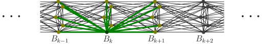
  Figure 1: Bracelet graph with $d/3=5$.

• Hiding a tightly-knit family. Start with $n/3$ disjoint triangles. Now, add an arbitrary bounded-degree graph (say, an expander) on these $n$ vertices. The resulting graph has constant triangle density, but most of the structure is irrelevant for a tightly-knit family.

5 Recovering a planted clustering

This section gives an algorithmic application of our decomposition procedure to recovering a “ground truth” clustering. We study the planted clustering model defined by Balcan, Blum, and Gupta [BBG13], and show that our algorithm gives guarantees similar to theirs. We do not subsume the results in [BBG13]. Rather, we observe that a graph problem that arises as a subroutine in their algorithm is essentially that of finding a tightly-knit family in a triangle-dense graph. Their assumptions ensure that there is (up to minor perturbations) a unique such family.

The main setting of [BBG13] is as follows. Given a set of points $V$ is some metric space, we wish to $k$-cluster them according to some fixed objective function, such as the $k$-median objective. Denote the optimal $k$-clustering by $\mathcal{C}$ and the value by $OPT$. The instance satisfies $(c,\epsilon)$-approximation-stability if for any $k$-clustering $\mathcal{C}^{\prime}$ of $V$ with objective function value at most $c\cdot OPT$, the “classification distance” between $\mathcal{C}$ and $\mathcal{C}^{\prime}$ is at most $\epsilon$. Thus, all solutions with near-optimal objective function value must be structurally close to $\mathcal{C}$.

In [BBG13, Lemma 3.5], an approximation-stable $k$-median instance is converted into a threshold graph. This graph $G=(V,E)$ contains $k$ disjoint cliques $\{X_{a}\}_{a=1}^{k}$, such that the cliques do not have any common neighbors. These cliques correspond to clusters in the ground-truth clustering, and their existence is a consequence of the approximation stability assumption. The aim is to get a $k$-clustering sufficiently close to $\{X_{a}\}$. Formally, a $k$-clustering $\{S_{a}\}$ of $V$ is $\Delta$-incorrect if there is a permutation $\sigma$ such that $\sum|X_{\sigma(a)}\setminus S_{a}|\leq\Delta$.

Let $B=V\setminus\bigcup_{a}X_{a}$. It is shown in [BBG13] that when $|B|$ is small, good approximations to $\{X_{a}\}$ can be found efficiently. From our perspective, the interesting point is that when $|B|$ is much smaller than $\sum_{a}|X_{a}|$, the threshold graph has high triangle density. Furthermore, as we prove below, the clusters output by the extraction procedure of Theorem 11 are very close to the $X_{a}$’s of the threshold graph.

Suppose we want a $k$-clustering of a threshold graph. We iteratively use the extraction procedure (from §3.3) $k$ times to get clusters $S_{1},S_{2},\ldots,S_{k}$. In particular, recall that at each step we choose a vertex $s_{i}$ with the current highest degree $d_{i}$. We set $N_{i}$ to be the $d_{i}$ neighbors of $s_{i}$ at this time, and $R$ to be the $d_{i}$ vertices with the largest number of triangles to $N_{i}$. Then, $S_{i}=\{i\}\cup N_{i}\cup R$. The exact procedure of Theorem 13, which includes cleaning, also works fine. Foregoing the cleaning step does necessitate a small technical change to the extraction procedure: instead of adding all of $R$ to $S$, we only add the elements of $R$ which have a positive number of triangles to $N_{i}$.

We use the notation $N^{*}(U)=N(U)\cup U$. So $N^{*}(X_{a})\cap N^{*}(X_{b})=\emptyset$, when $a\neq b$. Unlike [BBG13], we assume that $|X_{a}|\geq 3$. The following parallels the main theorem of [BBG13, Theorem 3.9], and the proof is similar to theirs.

Theorem 22.

The output of the clustering algorithm above is $O(|B|)$-incorrect on $G$.

Proof.

We first map the algorithm’s clustering to the true clustering $\{X_{a}\}$. Our algorithm outputs $k$ clusters, each with an associated “center” (the starting vertex). These are denoted $S_{1},S_{2},\ldots,$ with centers $s_{1},s_{2},\ldots,$ in order of extraction. We determine if there exists some true cluster $X_{a}$, such that $s_{1}\in N^{*}(X_{a})$. If so, we map $S_{1}$ to $X_{a}$. (Recall the $N^{*}(X_{a})$’s are disjoint, so $X_{a}$ is unique if it exists.) If no $X_{a}$ exists, we simply do not map $S_{1}$. We then perform this for $S_{2},S_{3},\ldots$, except that we do not map $S_{k}$ if we would be mapping it to an $X_{a}$ that has previously been mapped to. We finally end up with a subset $P\subseteq[k]$, such that for each $a\in P$, $S_{a}$ is mapped to some $X_{a^{\prime}}$. By relabeling the true clustering, we can assume that for all $a\in P$, $S_{a}$ is mapped to $X_{a}$. The remaining clusters (for $X_{a\notin P}$) can be labeled with an arbitrary permutation of $[k]\setminus P$.

Our aim is to bound $\sum_{a}|X_{a}\setminus S_{a}|$ by $O(|B|)$.

We perform some simple manipulations.

$$\bigcup_{a}\,(X_{a}\setminus S_{a}) = \bigcup_{a\in P}(X_{a}\setminus S_{a})\cup\bigcup_{a\notin P}(X_{a}\setminus S_{a})$$

$$= \bigcup_{a\in P}(X_{a}\cap\bigcup_{b<a}S_{b})\cup\bigcup_{a\in P}(X_{a}\setminus\bigcup_{b\leq a}S_{b})\cup\bigcup_{a\notin P}(X_{a}\setminus S_{a})$$

$$\subseteq \bigcup_{a}\,(X_{a}\cap\bigcup_{b<a}S_{b})\cup\bigcup_{a\in P}(X_{a}\setminus\bigcup_{b\leq a}S_{b})\cup\bigcup_{a\notin P}X_{a}.$$

So we get the following sets of interest.

• $L_{1}=\bigcup_{a}(X_{a}\cap\bigcup_{b<a}S_{b})=\bigcup_{b}(S_{b}\cap\bigcup_{a>b}X_{a})$ is the set of vertices that are “stolen” by clusters before $S_{a}$.

• $L_{2}=\bigcup_{a\in P}(X_{a}\setminus\bigcup_{b\leq a}S_{b})$ is the set of vertices that are left behind when $S_{a}$ is created.

• $L_{3}=\bigcup_{a\notin P}X_{a}$ is the set of vertices that are never clustered.

Note that $\sum_{a}|X_{a}\setminus S_{a}|=|\bigcup_{a}(X_{a}\setminus S_{a})|\leq|L_{1}|+|L_{2}|+|L_{3}|.$ The proof is completed by showing that $|L_{1}|+|L_{2}|+|L_{3}|=O(|B|)$. This will be done through a series of claims.

We first state a useful fact.

Claim 23.

Suppose for some $b\in\{1,2,\ldots,k\}$, $s_{b}\in N(X_{b})$. Then $N_{b}$ is partitioned into $N_{b}\cap X_{b}$ and $N_{b}\cap B$.

Proof.

Any vertex in $N_{b}\setminus X_{b}$ must be in $B$. This is because $N_{b}$ is contained in a two-hop neighborhood from $X_{b}$, which cannot intersect any other $X_{a}$. ∎

Claim 24.

For any $b$, $|S_{b}\cap\bigcup_{a>b}X_{a}|\leq 6|S_{b}\cap B|$.

Proof.

We split into three cases. For convenience, let $U$ be the set of vertices $S_{b}\cap\bigcup_{a>b}X_{a}$. Recall that $|S_{b}|\leq 2d_{b}$.

• For some $c$, $s_{b}\in X_{c}$: Note that $c\leq b$ by the relabeling of clusters. Observe that $S_{b}$ is contained in a two-hop neighborhood of $s_{b}$, and hence cannot intersect any cluster $X_{a}$ for $a\neq c$. Hence, $U$ is empty.

• For some (unique) $c$, $s_{b}\in N(X_{c})$: Again, $c\leq b$. By Claim 23, $d_{b}=|N_{b}|=|N_{b}\cap X_{c}|+|N_{b}\cap B|$. Suppose $|N_{b}\cap B|\geq d_{b}/3$. Then $|S_{b}\cap B|\geq|N_{b}\cap B|\geq d_{b}/3$. We can easily bound $|S_{b}|\leq 2d_{b}\leq 6|S_{b}\cap B|$.

  Suppose instead $|N_{b}\cap B|<d_{b}/3$, and hence $|N_{b}\cap X_{c}|>2d_{b}/3$. Note that $|N_{b}\cap X_{c}|$ is a clique. Each vertex in $N_{b}\cap X_{c}$ makes ${|N_{b}\cap X_{c}|-1\choose 2}\geq\binom{\lfloor 2d_{b}/3\rfloor}{2}$ triangles in $N_{b}$. On the other hand, the only vertices of $N_{b}$ that any vertex in $X_{a}$ for $a\neq c$ can connect to is in $N_{b}\cap B$. This forms fewer than ${\lfloor d_{b}/3\rfloor\choose 2}$ triangles in $N_{b}$. If ${\lfloor d_{b}/3\rfloor\choose 2}>0$, then $\binom{\lfloor 2d_{b}/3\rfloor}{2}>{\lfloor d_{b}/3\rfloor\choose 2}$.

  Consider the construction of $S_{b}$. We take the top $d_{b}$ vertices with the most triangles to $N_{b}$, and say we insert them in decreasing order of this number. Note that in the modified version of the algorithm, we only insert them while this number is positive. Before any vertex of $X_{a}$ ($a\neq b$) is added, all vertices of $N_{b}\cap X_{c}$ must be added. Hence, at most $d_{b}-|N_{b}\cap X_{c}|=|N_{b}\cap B|\leq|S_{b}\cap B|$ vertices of $\cup_{a\neq b}X_{a}$ can be added to $S_{b}$. Therefore, $|U|\leq|S_{b}\cap B|$.

• The vertex $s_{b}$ is at least distance $2$ from every $X_{c}$: Note that $N_{b}\subseteq S_{b}\cap B$. Hence, $|S_{b}|\leq 2d_{b}\leq 2|S_{b}\cap B|$. ∎

Claim 25.

For any $a\in P$, $|X_{a}\setminus\bigcup_{b\leq a}S_{b}|\leq|S_{a}\cap B|$.

Proof.

Since $a\in P$, either $s_{a}\in X_{a}$ or $s_{a}\in N(X_{a})$. Consider the situation of the algorithm after the first $a-1$ sets $S_{1},S_{2},\ldots,S_{a-1}$ are removed. There is some subset of $X_{a}$ that remains; call it $X^{\prime}_{a}=X_{a}\setminus\bigcup_{b<a}S_{b}$.

Suppose $s_{a}\in X_{a}$. Since $X^{\prime}_{a}$ is still a clique, $X^{\prime}_{a}\subseteq N_{a}$, and $(X_{a}\setminus\bigcup_{b\leq a}S_{b})$ is empty.

Suppose instead $s_{a}\in N(X_{a})$. Because $s_{a}$ has maximum degree and $X^{\prime}_{a}$ is a clique, $d_{a}\geq|X^{\prime}_{a}|-1$. Note that $|X^{\prime}_{a}\setminus S_{a}|$ is what we wish to bound, and $|X^{\prime}_{a}\setminus S_{a}|\leq|X^{\prime}_{a}\setminus N_{a}|$. By Claim 23, $N_{a}$ partitions into $N_{a}\cap X_{a}=N_{a}\cap X^{\prime}_{a}$ and $N_{a}\cap B$. We have $|X^{\prime}_{a}\setminus N_{a}|=|X^{\prime}_{a}|-|N_{a}\cap X_{a}|\leq d_{a}+1-|N_{a}\cap X_{a}|=|N_{a}\cap B|+1\leq|S_{a}\cap B|$. ∎

Claim 26.

$|L_{3}|\leq|B|+|L_{1}|$.

Proof.

Consider some $X_{a}$ for $a\notin P$. Look at the situation when $S_{1},\ldots,S_{a-1}$ are removed. There is a subset $X^{\prime}_{a}$ (forming a clique) left in the graph. All the vertices in $X_{a}\setminus X^{\prime}_{a}$ are contained in $L_{1}$. By maximality of degree, $d_{a}\geq|X^{\prime}_{a}|-1$. Furthermore, since $a\notin P$, $N_{a}\subseteq B$ implying $d_{a}\leq|S_{a}\cap B|-1$. Therefore, $|X^{\prime}_{a}|\leq|S_{a}\cap B|$. We can bound $\bigcup_{a\notin P}(X_{a}\setminus X^{\prime}_{a})\subseteq L_{1}$, and $\sum_{a\not\in P}|X^{\prime}_{a}|\leq|B|$, completing the proof. ∎

To put it all together, we sum the bound of Claim 24 and Claim 25 over $b\in[k]$ and $a\in P$ respectively to get $|L_{1}|\leq 6|B|$ and $|L_{2}|\leq|B|$. Claim 26 with the bound on $|L_{1}|$ yields $|L_{3}|\leq 7|B|$, completing the proof of Theorem 22.  ∎

6 Conclusions

This paper proposes a “model-free” approach to the analysis of social and information networks. We restrict attention to graphs that satisfy a combinatorial condition — constant triangle density — in lieu of adopting a particular generative model. The goal of this approach is to develop structural and algorithmic results that apply simultaneously to all reasonable models of social and information networks. Our main result shows that constant triangle density already implies significant graph structure: every graph that meets this condition is, in a precise sense, well approximated by a disjoint union of clique-like graphs.

Our work suggests numerous avenues for future research.

1. Can the dependence of the inter-cluster edge and triangle density on the original graph’s triangle density be improved?

2. The relative frequencies of four-vertex subgraphs also exhibit special patterns in social networks — for example, there are usually very few induced four-cycles [UBK13]. Is there an assumption about four-vertex induced subgraphs, in conjunction with high triangle density, that yields a stronger decomposition theorem?

3. Are there interesting additional conditions under which the decomposition into a tightly-knit family is essentially unique?

4. Which computational problems are easier for triangle-dense graphs than for arbitrary graphs? Just as planar separator theorems lead to faster algorithms and better heuristics for planar graphs than for general graphs, we expect our decomposition theorem to be a useful tool in the design of algorithms for triangle-dense graphs.

Acknowledgements

We are grateful for the helpful comments provided by Jon Kleinberg, Johan Ugander, and the anonymous ITCS reviewers.

References

- [AJB00] R. Albert, H. Jeong, and A.-L. Barabási. Error and attack tolerance of complex networks. Nature, 406:378–382, 2000.
- [BA99] A.-L. Barabasi and R. Albert. Emergence of scaling in random networks. Science, 286:509–512, 1999.
- [BBG13] M.-F. Balcan, A. Blum, and A. Gupta. Clustering under approximation stability. Journal of the ACM, 60(2):1068–1077, 2013.
- [BKM+00] A. Broder, R. Kumar, F. Maghoul, P. Raghavan, S. Rajagopalan, R. Stata, A. Tomkins, and J. Wiener. Graph structure in the web. Computer Networks, 33:309–320, 2000.
- [Bur04] R. S. Burt. Structural holes and good ideas. American Journal of Sociology, 110(2):349–399, 2004.
- [CF06] D. Chakrabarti and C. Faloutsos. Graph mining: Laws, generators, and algorithms. ACM Computing Surveys, 38(1), 2006.
- [CL02a] F. Chung and L. Lu. The average distances in random graphs with given expected degrees. Proceedings of the National Academy of Sciences, 99(25):15879–15882, 2002.
- [CL02b] F. Chung and L. Lu. Connected components in random graphs with given degree sequences. Annals of Combinatorics, 6:125–145, 2002.
- [Col88] J. S. Coleman. Social capital in the creation of human capital. American Journal of Sociology, 94:95–120, 1988.
- [CZF04] D. Chakrabarti, Y. Zhan, and C. Faloutsos. R-MAT: A recursive model for graph mining. In SIAM Conference on Data Mining, pages 442–446, 2004.
- [Fau06] Katherine Faust. Comparing social networks: Size, density, and local structure. Metodoloski zvezki, 3(2):185–216, 2006.
- [FFF99] M. Faloutsos, P. Faloutsos, and C. Faloutsos. On power-law relationships of the internet topology. In Proceedings of SIGCOMM, pages 251–262, 1999.
- [For10] S. Fortunato. Community detection in graphs. Physics Reports, 486:75–174, 2010.
- [FPP06] A. Ferrante, G. Pandurangan, and K. Park. On the hardness of optimization in power law graphs. In Proceedings of Conference on Computing and Combinatorics, pages 417–427, 2006.
- [FWVDC10] B. Foucault Welles, A. Van Devender, and N. Contractor. Is a friend a friend?: Investigating the structure of friendship networks in virtual worlds. In Extended Abstracts on Human Factors in Computing Systems, pages 4027–4032, 2010.
- [GN02] M. Girvan and M. Newman. Community structure in social and biological networks. Proceedings of the National Academy of Sciences, 99(12):7821–7826, 2002.
- [HL70] P. W. Holland and S. Leinhardt. A method for detecting structure in sociometric data. American Journal of Sociology, 76:492–513, 1970.
- [Kle00a] J. M. Kleinberg. Navigation in a small world. Nature, 406:845, 2000.
- [Kle00b] J. M. Kleinberg. The small-world phenomenon: An algorithmic perspective. In Proceedings of the Symposium on Theory of Computing, pages 163–170, 2000.
- [Kle02] J. M. Kleinberg. Small-world phenomena and the dynamics of information. In Advances in Neural Information Processing Systems, volume 1, pages 431–438, 2002.
- [KRR+00] R. Kumar, P. Raghavan, S. Rajagopalan, D. Sivakumar, A. Tomkins, and E. Upfal. Stochastic models for the web graph. In Proceedings of Foundations of Computer Science, pages 57–65, 2000.
- [LAS+08] H. Lin, C. Amanatidis, M. Sideri, R. M. Karp, and C. H. Papadimitriou. Linked decompositions of networks and the power of choice in Polya urns. In Proceedings of the Symposium on Discrete Algorithms, pages 993–1002, 2008.
- [LCK+10] J. Leskovec, D. Chakrabarti, J. M. Kleinberg, C. Faloutsos, and Z. Ghahramani. Kronecker graphs: An approach to modeling networks. Journal of Machine Learning Research, 11:985–1042, 2010.
- [LLDM08] J. Leskovec, K. Lang, A. Dasgupta, and M. Mahoney. Community structure in large networks: Natural cluster sizes and the absence of large well-defined clusters. Internet Mathematics, 6(1):29–123, 2008.
- [LT79] R. J. Lipton and R. E. Tarjan. A separator theorem for planar graphs. SIAM Journal on Applied Mathematics, 36(2):177–189, 1979.
- [MS10] A. Montanari and A. Saberi. The spread of innovations in social networks. Proceedings of the National Academy of Sciences, 107(47):20196–20201, 2010.
- [New01] M. E. J. Newman. The structure of scientific collaboration networks. Proceedings of the National Academy of Sciences, 98(2):404–409, 2001.
- [New03] M. E. J. Newman. Properties of highly clustered networks. Physical Review E, 68(2):026121, 2003.
- [New06] M. E. J. Newman. Finding community structure in networks using the eigenvectors of matrices. Physical Review E, 74(3):036104, 2006.
- [RS86] N. Robertson and P. D. Seymour. Graph minors III: Planar tree-width. Journal of Combinatorial Theory, Series B, 36(1):49–64, 1986.
- [SCW+10] A. Sala, L. Cao, C. Wilson, R. Zablit, H. Zheng, and B. Y. Zhao. Measurement-calibrated graph models for social network experiments. In Proceedings of the World Wide Web Conference, pages 861–870. ACM, 2010.
- [SPK13] C. Seshadhri, A. Pinar, and T. G. Kolda. Fast triangle counting through wedge sampling. In Proceedings of the SIAM Conference on Data Mining, 2013.
- [SPR11] V. Satuluri, S. Parthasarathy, and Y. Ruan. Local graph sparsification for scalable clustering. In Proceedings of ACM SIGMOD, pages 721–732, 2011.
- [Sze78] E. Szemerédi. Regular partitions of graphs. Problèmes combinatoires et théorie des graphes, 260:399–401, 1978.
- [UBK13] J. Ugander, L. Backstrom, and J. Kleinberg. Subgraph frequencies: Mapping the empirical and extremal geography of large graph collections. In Proceedings of World Wide Web Conference, pages 1307–1318, 2013.
- [UKBM11] J. Ugander, B. Karrer, L. Backstrom, and C. Marlow. The anatomy of the facebook social graph. Technical Report 1111.4503, Arxiv, 2011.
- [VB12] J. Vivar and D. Banks. Models for networks: A cross-disciplinary science. Wiley Interdisciplinary Reviews: Computational Statistics, 4(1):13–27, 2012.
- [WF94] S. Wasserman and K. Faust. Social Network Analysis: Methods and Applications. Cambridge University Press, 1994.
- [WS98] D. Watts and S. Strogatz. Collective dynamics of ‘small-world’ networks. Nature, 393:440–442, 1998.