I hear, I forget. I do, I understand:
a modified Moore-method mathematical statistics course

I hear, I forget. I do, I understand:
a modified Moore-method mathematical statistics course

Abstract

Moore introduced a method for graduate mathematics instruction that consisted primarily of individual student work on challenging proofs [jone:1977]. cohe:1992 described an adaptation with less explicit competition suitable for undergraduate students at a liberal arts college. This paper details an adaptation of this modified Moore-method to teach mathematical statistics, and describes ways that such an approach helps engage students and foster the teaching of statistics.

Groups of students worked a set of 3 difficult problems (some theoretical, some applied) every two weeks. Class time was devoted to coaching sessions with the instructor, group meeting time, and class presentations. R was used to estimate solutions empirically where analytic results were intractable, as well as to provide an environment to undertake simulation studies with the aim of deepening understanding and complementing analytic solutions. Each group presented comprehensive solutions to complement oral presentations. Development of parallel techniques for empirical and analytic problem solving was an explicit goal of the course, which also attempted to communicate ways that statistics can be used to tackle interesting problems. The group problem solving component and use of technology allowed students to attempt much more challenging questions than they could otherwise solve.

Keywords: capstone course, empirical problem solving, intermediate statistics, R software, RStudio integrated development environment, reproducible analysis, simulation studies, statistical computing, statistical education

1 Introduction

In this paper, an implementation of a mathematical statistics course is described with the goal of developing a combination of analytic and empirical problem-solving skills through the solution of challenging problems and complex case studies. The course, offered at the Department of Mathematics and Statistics at Smith College in spring 2007 and spring 2011, adapted the approach of R.L Moore [jone:1977], using modifications suggested by cohe:1992. A similar mathematical statistics course is described by mclo:2008.

In the next subsection, recent developments in statistics education are described, followed by an overview of the modified Moore-Cohen method. Section 2 describes specific details of the course, Section 3 provides two example problems (with empirical as well as analytic solutions), Section 4 describes grading and assessment while Section 5 provides additional discussion and closing thoughts.

1.1 Developments in statistical education

Extensive curricular reforms in undergraduate statistics education have transformed our programs and courses in recent decades [cobb:1992, moor:cobb:1995, cobb:2011]. The Guidelines for Assessment and Instruction for Statistics Education (GAISE) report [gaise], which succinctly described these changes, recommended that introductory statistics courses:

• Emphasize statistical literacy and develop statistical thinking,

• Use real data,

• Stress conceptual understanding rather than mere knowledge of procedures,

• Foster active learning in the classroom,

• Use technology for developing conceptual understanding and analyzing data, and

• Use assessments to improve and evaluate student learning.

Other related efforts have attempted to broaden the types of questions that statistics students grapple with [brow:kass:2009, goul:2010], increase the use of case studies [barr:tamb:1980, nola:spee:2000, nola:2003] and take advantage of sophisticated computing technologies and environments such as R [ihak:gent:1996] or Matlab [kapl:2003] to buttress understanding of statistical concepts [butt:nola:2001, nola:temp:2003, hort:brow:2004, froe:2008, nola:temp:2010, laza:2011].

The mathematical statistics course has undergone many transformations during this same period. A lively panel in 2003 with the provocative title “Is the Math Stat Course obsolete?” [obsolete] provided a glimpse into ways that this intermediate level statistics course is adapting to a changing landscape. One idea raised was that the math stat course (still a common entry point to the field for many students studying mathematics) should convey the excitement of the discipline (“even if they don’t go on [in statistics], we want them to leave thinking statistics is interesting”). Another was that modeling, computing and problem-solving are key components of such a course.

cobb:2011 provides a series of capsule summaries of innovations in the teaching of mathematical statistics, and discusses key tensions that underlie our courses in terms of what we want students to learn:

Surely the most common answer must be that we want our students to learn to analyze data, and certainly I share that goal. But for some students, particularly those with a strong interest and ability in mathematics, I suggest a complementary goal, one that in my opinion has not received enough explicit attention: We want these mathematically inclined students to learn to solve methodological problems. I call the two goals complementary because, as I shall argue in detail, there are essential tensions between the goals of helping students learn to analyze data and helping students learn to solve methodological problems.

For a ready example of the tension, consider the role of simple, artificial examples. For teaching data analysis, these “toy” examples are often and deservedly regarded with contempt. But for developing an understanding of a methodological challenge, the ability to create a dialectical succession of toy examples and exploit their evolution is critical (p. 32).

1.2 Moore and Cohen methods

Moore was noted [halm:1985] for quoting the Chinese proverb I hear, I forget. I see, I remember. I do, I understand. He provided classes with a list of definitions and theorems which they would subsequently prove individually and then share with the rest of the class. Competition was a key driving force in the course [jone:1977], with efforts to ensure that student background was as homogeneous as possible. The overall goal was to build student capacity to create structure from an axiomatic basis and communicate this to others. chri:2009 described possible evaluations and assessment of Moore method mathematics courses.

cohe:1992 modified Moore’s approach using three guiding principles:

• Students understand better and remember longer what they discover themselves than what is told to them,

• People master an idea thoroughly when they teach it to someone else, and

• Effective writing and clear thinking are inextricably linked (p. 474).

A fourth principle incorporated in this mathematical statistics course involved the use of R [r-ref] and RStudio (an open source integrated development environment for R) to facilitate parallel empirical and analytic problem solving techniques.

Much of the class time is spent with students working as a group and individually to solve sets of challenging problems, writing up solutions, and presenting them to the class as a whole. While each group tackled problems from each of the major units of the course, group members would tend to learn their assigned problems in more detail and rely on their classmates to convey understanding of the other problems.

The Moore and Cohen approaches deal more with pedagogy than with curriculum. Moore used his method to teach proofs in topology. Cohen used his method for linear algebra. Here we borrow Cohen’s pedagogy for a course in mathematical statistics. Students are not given theorems to prove as in Moore’s courses; instead they are given challenging problems to solve.

These problems are chosen according to four criteria. The first two are critical to the pedagogy: each problem should be easy to grasp, and each should be hard enough that solving it poses a genuine challenge. The first criterion helps ensure that all students in a group can participate; the second helps ensure that stronger students will not be able to cut off discussion with a quick solution.

A third criterion is that the problems should have links to actual applications. This is in the spirit of the GAISE recommendations.

Fourth, the problems should lend themselves to parallel and complementary pairs of solutions, one based on simulation and the other based on theory. The parallel solutions constitute a recurring theme to the course, one that is central to the curriculum. This criterion is in some ways incidental to the pedagogy, although it helps ensure that students with different strengths and backgrounds can contribute actively to group work.

2 Details of the course

For the sections (officially titled “Seminar in Mathematical Statistics”) taught by the author in Spring 2007 and Spring 2011, the class met three times per week for 80 minutes per session for thirteen weeks.

While the only required prerequisite for the class was probability, most students in the course had also taken introductory statistics and linear algebra. No specific knowledge of statistics was assumed. At the beginning of the course, the students took the 40 item multiple choice CAOS (Comprehensive Assessment of Outcomes in a first statistics course) test [delm:garf:2006]. While designed to assess student reasoning after a first course in statistics (and not a mathematical statistics class), the CAOS focuses on conceptual understanding of variability and uncertainty. The average score for the mathematical statistics students on the CAOS pre-test was 67.2% correct with a standard deviation of 13.6% (values ranged from 43% to 90%).

The structure of the course included (almost) no lectures. Instead, the material was broken down into a number of problem sets. These questions were designed to be sufficiently difficult to provide a challenge to students, but still amenable (with some assistance) to solution.

During the first offering, four groups of 3 students were created, with seven groups of 3 students for the second offering. Each group would work a different set of problems for each problem set (with an occasional problem assigned to all groups). Throughout the semester, these groups were reshuffled twice, with no two individuals being in the same group twice. The re-balancing helped to address issues with groups that consisted of only weak students (as well as to provide a release valve for problems with group dynamics).

Most class sessions consisted of a series of “coaching” sessions several days after the initial presentation of the problems. These coaching sessions, described in detail in cohe:1992, are critical in helping to guide students towards the desired solution without providing the answer. All students in a group attended a given coaching session, and discussed their preliminary attempts at the problems. In some cases they may have solved their problems. More commonly additional guidance was needed for them to make progress or to elaborate on their solutions. Early on in the course, much of this coaching involved support and scaffolding for the use of computing (to allow them to gradually build their skills in terms of simulation and exploration).

Each student created a draft of their preliminary solution in preparation for a second coaching session. To ensure that all students were engaged and making good faith efforts, these were reviewed by the instructor. One per group was graded in detail, to provide general feedback for all students.

The second coaching session was used to help answer any remaining questions and assist with preparations of the solutions (“weekly papers”). Other assistance was provided outside of the regular class meeting times by email or during office hours.

Before the final class session for a given set of problems, each group created a single clear and comprehensive solution, which was made available to the class. Finally, each group gave a 15 minute oral presentation that reviewed their solution, with questions and answers as needed.

2.1 Textbooks and topics

The approach suggested by cohe:1992 to teach analysis of linear algebra provides students several pages of axioms, definitions, theorems and problems. This serves as the foundation from which all of the remaining material is derived. Because of the need for more extensive material to support student work in a range of mathematical statistical topics, the text by rice:1995 was used for background reading as well as the source of many of the problems. In addition, several modules (including case studies with advanced data analysis) were integrated from nola:spee:2000.

The course began with a series of challenging probability problems, covering selected topics and highlights from Chapters 1 through 5 of rice:1995. The next set of problems related to descriptive and graphical visualization (covering Chapter 10 of rice:1995 and the Maternal smoking and infant health module from nola:spee:2000). Two sets of problems were devoted to estimation and the bootstrap (Chapter 8 of rice:1995 and the Patterns in DNA and Who plays video games? modules from nola:spee:2000). Testing hypotheses and assessing goodness of fit (Chapter 9 of rice:1995) comprised two sets of problems, while Chapter 10 was used as a basis for a set on two sample comparisons. The first time the course was offered, it closed with a set of problems entitled Bayesian inference: a big idea, based loosely on Chapter 15 of rice:1995 and Section 2.5 of lavi:2007, while the second offering closed with precursors of informal inference and simulation studies of inference rules [wild:2010].

2.2 Real data and mathematical statistics

While the course did not focus on advanced analysis of multivariate datasets, real data was regularly incorporated into the course, primarily as a component of problems assigned to the students throughout the semester. The textbooks by Rice as well as Nolan & Speed are notable for the number and variety of motivating examples provided throughout, including the exercises. As an example, students might be asked to find the method of moments estimator for $\theta$ for a Pareto distribution with known scale parameter $x_{0}$, and compare this to the maximum likelihood estimator for $\theta$. After finding the analytic results, and simulating to compare the variance of the estimators, they would be asked to calculate and interpret the sample statistic using data from an economic survey. Another set of problems related to the analysis of cell probabilities expected by genetic theories, through estimation of underlying parameters. Students were assessed both on their ability to report in context on the underlying applied statistical question, as well as on the relevant statistical derivations or simulations that they carried out.

As outlined by the GAISE guidelines, use of real data is essential to the introductory course, and central also to any statistics curriculum as a whole. Nevertheless, for certain individual courses that serve as elements of a larger statistics curriculum, real data may be less essential. There is an inherent complementarity between analysis of data using existing methods and the development of new methods [cobb:2011]. We need a curriculum that teaches students to engage, appreciate and enjoy both data analytic and methodological challenges. In a course such as the one described here, although connections to real data are important, the balance is weighted towards problems of a more abstract sort.

2.3 Technology

This approach would not be feasible without the use of computing technology to facilitate analysis and simulation. R [ihak:gent:1996] and RStudio (http://rstudio.org) provided a flexible and adaptable environment for exploration [hort:brow:2004, prui:2011].

RStudio is an open-source integrated development environment that provides a consistent and powerful interface for R (an open source general purpose statistical package, http://r-project.org) that is easier to install, learn and run than standard R. LaTeX [latex] within the Sweave [leis:2002] system was used as the formatting environment for the solutions, with an annotated example distributed to all students during the initial class meeting. This included examples of tables, figures, cross referencing, bibliography and other useful attributes. Submissions were made available to students as both Sweave source and PDF files to allow students to borrow working code. RStudio is particularly attractive because it simplifies the user interface and has tightly integrated support for Sweave (including a single button click to Compile PDF from the source document). In future offerings, the Markdown system within the knitr package [knitr] will be used, as it provides simplified functionality and does not require knowledge of LaTeX.

The course intentionally introduced students to concepts of reproducible analysis [gent:temp:2007], where computation, code and results of an analysis are integrated. Being able to re-run a set of simulations and regenerate a report with a single click is a powerful motivator for students used to error-prone processes of cutting and pasting output and figures. Reproducible analysis systems are becoming standard in industry and academia, have the potential to help ensure better statistical analysis, and should be incorporated in the statistics curriculum.

To help simplify the learning curve for these somewhat complex systems, a number of examples and idioms were provided by the instructor, to help build students’ repertoire of useful techniques to attack problems. Students were encouraged to write their initial solutions using pseudo-code (an informal description that could later be turned into working R code). These were also posted to the course management system to facilitate re-use in other problems and settings.

3 Example problems and solutions

To give a better sense of the course, we describe two problems that were completed by the students, along with model solutions and commentary (additional examples are found in the online supplement). Each group would generally work 3 or 4 problems per assignment.

These problems feature both empirical (simulations in R) and analytic (closed-form) solutions by the groups. They range from easier to more challenging, but illustrate the approaches taken by students in three separate application areas. The general level of difficulty is similar to that of rice:1995.

3.1 Pooled blood sera sampling

It is known that 5% of the members of a population have disease X, which can be discovered by a blood test (that is assumed to perfectly identify both diseased and nondiseased populations). Suppose that $N$ people are to be tested, and the cost of the test is non-trivial. The testing can be done in two ways: (A) Everyone can be tested separately; or (B) the blood samples of $k$ people are pooled to be analyzed. Assume that $N=nk$ with $n$ an integer. If the test is negative, all the people tested are healthy (that is, just this one test is needed). If the test result is positive, each of the $k$ people must be tested separately (that is, a total of $k+1$ tests are needed for that group).

Questions:

1. For fixed $k$ what is the expected number of tests needed in (B)?

2. Find the $k$ that will minimize the expected number of tests in (B).

3. Using the $k$ that minimizes the number of tests, on average how many tests does (B) save in comparison with (A)? Be sure to check your answer using an empirical simulation.

3.1.1 Empirical (simulation-based) solution

We attempted to gain a better understanding of the problem by simulation. First, we set $k=10$, $n=500$ and $P(\textrm{infected})=p=0.05$ (refer to Figure 1 for code). Given these specific values for each of the variables, we found the expected number of tests to be approximately 2501.9. We then used this value to help us check our analytic solution.

Next, we tried different values of $k$ and $n$ such that $N$ (the number of people to be tested) equaled 5000. We did this to find the value of $k$ that minimized the expected number of tests. Given that $N=5000$, possible integer values for $k$ were 2, 4, 5, 8, and 10. We found the expected number of tests for each of these $k$ values, respectively were 2988.7, 2178.9, 2126.5, 2306.2, and 2501.9. For this example, the minimum value is found when $k=5$.

numsim = 1000
p = 0.05       # probability of infection
k = 10         # size of pool
n = 500        # number of pools
N = n*k        # total number of people

# for Approach (A), E[# tests] = N
# for Approach (B), find E[# tests] if pooled?
res = numeric(numsim)    # stash results
for (i in 1:numsim) {
  disease = rbinom(N, size=1, prob=p)
  poolmat = matrix(disease, nrow=k, ncol=n)
  Y = apply(poolmat, 2, sum)>=1
  res[i] = n+sum(Y)*k
}
mean(res)
sd(res)
curve(N/x+x*(N/x)*(1-(1-p)^x), xlab="number in pool (k)",
  ylab="expected number", from=2, to=10)

Figure 1: R code to generate empirical estimates using Approach (B)

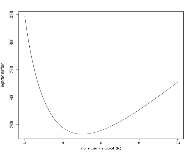
Figure 2: Display of expected number of blood tests required as a function of pool-size ($k$), with $N=5000,p=0.05$

3.1.2 Analytic (closed-form) solution

Approach (A): the expected number of tests needed is $E[T_{A}]=N=n*k,$ because we would be testing each individual exactly once.

For Approach (B):

1. Let $Y$ = the # of pools infected and $T_{B}$ = the total number of tests needed. Assuming independence, we have that $E[Y]=n(1-.95^{k})$ and $E[T_{B}]=n+kE[Y]=n+k(n(1-.95^{k}))$. With $N=5000$ people, this simplifies to: $E[T_{B}]=5000(1/k+(1-.95^{k}))$. When $k=10$, $n=500$ and $P(\textrm{infected})=p=0.05$, $E[T_{B}]=2506.3$, which closely matches the results from the simulation.

2. We find the derivative of $E[T_{B}]$ with respect to $k$ and solve (using a symbolic mathematics package such as Maple or Wolfram Alpha), which yields a positive solution of $k=5.022$ (see Figure 2). When $k=5$,

   $$E[T_{B}]=n+5(n(1-.95^{5}))=n+1.13n=2.13n=2130.$$

   This result is similar to that shown in the empirical simulations.

3. We compare the two expected number of tests needed for each of the approaches when $k=5$ and $p=0.05$:

   $$E[T_{A}]/E[T_{B}]=5n/2.13n=2.35.$$

   Approach (A) requires an average of 2.35 times the number of tests than Approach (B). Figure 2 demonstrates that this ratio is greater than 1 for pool sizes between 2 and 10, given a prevalence of $0.05$.

3.1.3 Commentary

This problem was part of a series of probability questions at the start of the course. While more efficient programming approaches could be used, the empirical solution features a number of idioms and tricks of the trade that are repeated throughout the class.

This example demonstrates a setting where the analytic solution is straightforward using basic properties of expectations, but where the empirical solution provides a useful check on the results. This type of question helps students build confidence in using knowledge from the prerequisite course in new ways.

3.2 Sampling from a probability distribution

Questions [from evan:rose:2004]:

1. Is it possible to find a tractable expression for the cdf of a distribution with density given by: $f(y)=c(1+|y|)^{3}\exp(-y^{4}),$ where $c$ is a normalizing constant and $y$ is defined on the whole real line? If not, can you find $c$?

2. Show how to generate a sample of observations from this distribution.

3. Describe how this is useful in Bayesian inference.

3.2.1 Solution

1. While it is possible to find a closed-form solution for the cdf of this distribution it is not easily solvable. Note that because the density is a function of the absolute value of $y$, the integral can be broken into two symmetric parts. To find $c$, we evaluate twice the integral from $[0,\infty)$ in R:

   > f = function(x){exp(-x^4)*(1+abs(x))^3}
   > integral = integrate(f, 0, Inf)
   > 2 * integral$value
   [1] 6.809611
   

   Hence $c=1/6.809611\cong 0.15.$

2. We created a Markov Chain Monte Carlo sampler, using the Metropolis-Hastings algorithm. The premise for this algorithm is that it chooses proposal probabilities so that after the process has converged draws are generated from the desired distribution. A further discussion for enthusiasts can be found on Page 610 of evan:rose:2004. We find the acceptance probability $\alpha(x,y)$ in terms of two densities, our $f(y)$ and $q(x,y)$, a normal proposal density with mean $x$ and variance 1, so that

   $$\alpha(x,y) = \mathrm{min}\left\{1,\frac{f(y)q(y,x)}{f(x)q(x,y)}\right\}$$

   $$= \mathrm{min}\left\{1,\frac{c\exp{(-y^{4})}(1+|y|)^{3}(2\pi)^{-1/2}\exp{(-(y-x)^{2}/2)}}{c\exp{(-x^{4})}(1+|x|)^{3}(2\pi)^{-1/2}\exp{(-(x-y)^{2}/2)}}\right\}$$

   $$= \mathrm{min}\left\{1,\frac{\exp{(-y^{4}+x^{4})}(1+|y|)^{3}}{(1+|x|)^{3}}\right\}$$

   Pick an arbitrary value for $X_{1}$. The Metropolis-Hastings algorithm then computes the value $X_{n+1}$ as follows:
   1. Generate $Y_{n+1}$ from a normal($X_{n}$, 1).
   2. Let $y=Y_{n+1}$, compute $\alpha(x,y)$ as before.
   3. With probability $\alpha(x,y)$, let $X_{n+1}=Y_{n+1}=y$ (use proposal value). Otherwise, with probability $1-\alpha(x,y)$, let $X_{n+1}=X_{n}=x$ (keep previous value).
   

   The code (displayed in Figure 3), uses the first 100,000 iterations as a burn-in period, then generates 100,000 samples. A histogram is displayed in Figure 4.

3. The Metropolis-Hastings algorithm is a form of Markov Chain Monte Carlo (MCMC) and is particularly attractive when the posterior density function does not have a familiar integral (such as when $f(x)$ is a posterior density that does not correspond to a conjugate prior).

   Simulation is a central part of applied Bayesian analysis, because of the relative ease with which samples can be generated from a probability distribution, even when the density function cannot be explicitly integrated (see page 25 of gelm:carl:2004).

x = seq(from=-3, to=3, length=200)
pdfval = 1/6.809610784*exp(-x^4)*(1+abs(x))^3
par(mfrow=c(2, 1)); plot(x, pdfval, type="n"); lines(x, pdfval)
title("Actual pdf")

alphafun = function(x, y) { return(exp(-y^4+x^4)*(1+abs(y))^3*
   (1+abs(x))^-3) }
numvals = 100000; burnin = 100000
i = 1
xn = 3 # arbitrary value to start
while (i <= burnin) {
   propy = rnorm(1, mean=xn, sd=1)
   alpha = min(1, alphafun(xn, propy))
   unif = runif(1) < alpha
   xn = unif*propy + (1-unif)*xn
   i = i + 1
}
i = 1
res = rep(0, numvals)
while (i <= numvals) {
   propy = rnorm(1, mean=xn, sd=1)
   alpha = min(1, alphafun(xn, propy))
   unif = runif(1) < alpha
   xn = unif*propy + (1-unif)*xn
   res[i] = xn
   i = i + 1
}
hist(res, nclass=20, main="Metropolis-Hastings samples",
   xlab="x", freq=FALSE)

Figure 3: R code to generate Metropolis-Hastings samples

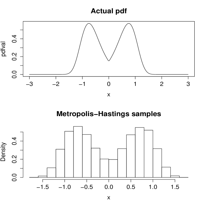
Figure 4: True density and simulated draws from probability distribution

3.2.2 Commentary

This problem was taken from the final set of problems, entitled Bayesian statistics: a big idea, which was intended to introduce students to more sophisticated simulations that are necessary to get answers for more complex models. Because the students had no prior experience with MCMC, a preliminary mini-lecture on the topic was provided along with supporting readings from lavi:2007. This included some classic examples with conjugate priors. Throwing the nasty density function at students was initially off-putting, but it helped to motivate MCMC methods and introduce Bayesian ideas and methods. The goal of this section was to give students a glimpse into a flexible and sophisticated set of models that can tackle problems far outside the realm of a traditional math stat class.

4 Grading and assessment

Assessment of students in the course was done in several ways. Students completed 7 sets of problems over the course of the semester (each one approximately 2 weeks apart). Grades on preliminary solutions and weekly papers constituted 35% of the grade, with class participation, attendance and oral presentations an additional 20%. Two midterm exams accounted for 40% while 5% reflected good faith effort towards completion of low-stakes online assessments. The midterm exams had in-class and take-home components. They included problems similar to those undertaken by the groups, albeit with simpler solutions.

An informal mid-semester evaluation was undertaken approximately halfway through the course. For the first offering of the course, a colleague met with the class during the last 15 minutes of a class session (without the instructor present). Feedback from this assessment indicated great worries about the structure of the take-home midterm (would the problems be as hard as Rice?) and queries about other forms of assessment.

For the second offering, a more formal evaluation was undertaken where a staff member from the college learning center spent the last 20 minutes of a class session with students in focus groups. The students appreciated the structure of the course and the opportunities for revision. They “like that we get lectures on background, the collaboration and group work” and “like that we do analytic and empirical solutions.” Students sought more input from the instructor, with a desire for more lectures to “put things into perspective.” Some students suggested that the instructor “tell us what are the key points to absolutely know from each problem set.” The final question from the focus groups related to the students’ roles as learners. Students revealed that they understand that they have to prepare more thoroughly for class, improve their own class participation and assume additional responsibilities outside of class. The students acknowledged that they should read the text more carefully, read other groups’ problems before the presentations, and “try harder” with Rice.

The outside evaluator summarized the report with the following quote:

As you made clear to me in our discussion, although your students may want you to tell them “the key points to absolutely know,” you believe strongly that they must work their way towards knowledge mastery in this course. To assist them in achieving this end, you have structured the course in ways that require them to work individually and collaboratively–with guidance from you–as they become more expert and reflective learners.

Many of your students are uneasy with this approach and unsure of themselves: they want to know the right answers, the correct way to think, hence their request for more input from you. Their unease marks them as less sophisticated about real learning and/or timid about undertaking independent intellectual journeys. You might have an explicit discussion with your students about your pedagogy and your learning goals for them. I suspect they would be quite responsive to this kind of communication given their high regard for you and this course: they know you believe in them. And, since their answers to the third question reveal that they are aware of their own responsibilities as students, you could also use this discussion to reinforce their own good insights on becoming more active and inquisitive learners.

The students also completed the CAOS post-test at the end of the class, with a mean of 72.5% correct (sd=13%, min=43%, max=90%). There was a statistically significant increase in scores compared to the pre-test (paired t-test p=0.01, df=30, 95% confidence interval from 1.4 to 9.2 point increase). Figure 5 displays the relationship between pre and post scores (with a solid scatterplot smoother plus dashed $POST=PRE$ line). There is some indication of larger improvement for students with lower pre-test scores, which is consistent with a ceiling effect. Given that the CAOS test is intended to assess outcomes from a first course, this is not surprising.

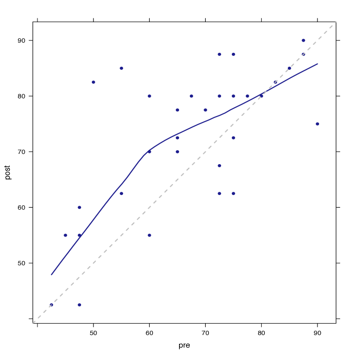
Figure 5: Relationship between student outcomes on the CAOS (Comprehensive Assessment of Outcomes in a first Statistics course) from the class in 2007 and 2011 (plus smoothed line and $POST=PRE$ line).

5 Discussion

This paper describes an implementation of a modified Moore-Cohen method mathematical statistics course at an undergraduate liberal arts college. The course featured a series of challenging problems, some theoretical, others data-driven, designed to help teach mathematical statistics using applications. A key idea is that the use of technology (R/RStudio and reproducible analysis tools) has opened up new possibilities.

An attractive aspect of the proposed course was how it intentionally dovetailed with the GAISE recommendations [gaise]. In particular, it was designed to encourage statistical thinking through empirical problem solving, use real data to motivate methods, stress conceptual understanding, foster active learning and use technology to develop conceptual understanding. The course is consistent with the American Statistical Association guidelines for statistics programs [asa-undergrad], which call for students to develop effective technical writing, presentation skills, teamwork and collaboration, in addition to knowledge of statistics.

5.1 Comparisons, advantages and limitations

This approach differs significantly from the traditional Moore-method, which was developed for a definition-theorem-proof type course and relies primarily on individual work and competition as a motivator. The modified Moore-Cohen method uses group work to facilitate engagement, with stronger students able to plunge more deeply into their solutions while still ensuring that weaker students can receive assistance as needed. This modification might be better thought of as a species split-off, where rather than competing, students are supported to go beyond their expectation and discover something in themselves.

A primary challenge of teaching is to engage students in the material being studied. cohe:1992 noted that the method effectively raises the level of communication between students and that most students are stimulated by the change from passive to active learning. laza:2011 described the importance of capstone courses in statistics. Structuring the class with multiple, challenging problems that were not amenable to quick individual solution helped to achieve the goals of a capstone. This includes getting students to grapple with real-world problems, helping them develop capacities to work effectively in groups, augmenting their ability to compute to extend their problem-solving abilities, and helping them to sharpen their abilities to communicate the complexity and power of statistical methods. The course also dovetails with other efforts to involve students in interdisciplinary research projects [legl:2010], which tend to focus on larger, more complex datasets in the context of a client discipline.

While no formal assessment of the course was undertaken, student feedback from less formal appraisals was generally positive. Students found the approach to be challenging, particularly at the beginning of the semester when they were confronted with simultaneously learning R/RStudio, LaTeX/Sweave, empirical problem solving techniques as well as oral and written presentation skills. The particular technical challenges of learning new packages and systems quickly receded, and the primary challenge related to answering difficult questions and learning new material, concepts and statistical methods.

A limitation of problem or case-based courses is that they typically cover fewer topics in more depth. That was true for this course, which had more constrained coverage goals than the traditional math stat class (though most of the typical key concepts were covered). In addition, students would be expected to have variable mastery of particular topics that were included, since they engaged in the problems that their group was assigned at an intense level, but had more passive involvement in the problems that other groups presented. The combination of written and oral presentation of solutions from other groups was designed to minimize these disparities. Ideally students would emerge from the course with useful capacities (such as ability to compute with data, simulate to approximate answers, and communicate orally and through their writing) that would allow them to fill any gaps in their knowledge and succeed in a graduate level course.

Classes that include group work as a component of assessments often have group dynamic issues, and this course was no exception. In general there was a positive sense of community and engagement which flowed from the group-based workload. Knowing that the groups would be reshuffled twice helped as well. Focusing much of the work in groups allowed students to tackle far more challenging questions than they could solve individually and also modeled a common post-college work environment. Several students have provided anecdotal reports of the value of learning tools for statistical computing and reproducible analysis.

There are other challenges to use of this method for teaching the mathematical statistics courses. The enrollments were 12 and 20 students in Spring 2007 and Spring 2011, respectively. While scaling to course sizes of 30–40 students would be straightforward, larger class sizes would require different systems and structures. These might include multiple sections taught with some common mini-lectures, doubling up on problems or student support for computing. The time commitment was comparable to a standard course, due to the extensive coaching and preparation, despite the fact that formal lectures were relatively short (generally at the start of each new topic).

5.2 Use of technology

Empirical (simulation-based) estimation complements analytic solutions, and can often allow approximate solution of extremely challenging problems. Besides providing a useful check on analytic answers, these simulations can help with insights into how to solve a problem. R and RStudio serve as a flexible and powerful environment for such exploration.

A number of technologies were prominently featured in the course. These included extensive use of LaTeX and R. Reproducible analysis (the Sweave system [leis:2002] as implemented within RStudio) greatly facilitated integration of commands, output and graphics, and led to better facility for students to undertake analyses outside the course. This scaffolding also helped to move students from a “point and click” approach to statistical analysis towards a more flexible scripting interface. Further discussion of how to integrate reproducible analysis and effective mechanisms to build students’ ability to “compute with data” are important issues but lie somewhat outside the scope of this paper.

Other courses may find the use of R and RStudio for simulation and approximation of analytic solutions to be helpful, without the Moore-method approach. The new text by prui:2011 features such a presentation.

5.3 Closing thoughts

cobb:2011 argues that the profession needs two types of statisticians: those with the capacity to appropriately analyze and interpret data, as well as those with interest in devising novel solutions to methodological challenges. Teaching mathematical statistics in this manner has the potential to foster engagement by presenting students with extended glimpses of the excitement of developing statistical procedures to solve challenging problems [nola:temp:2010]. This approach could also serve as a model for other intermediate and advanced undergraduate statistics classes. This method may also be relevant for the teaching of similar quantitative courses in other disciplines.

Online Appendix: Additional Example Problems

I hear, I forget. I do, I understand:
a modified Moore-method mathematical statistics course

The following material is proposed as an online appendix.

5.4 Estimating $\sigma$ using IQR

Assume that we observe $n$ iid observations from a normal distribution. Questions:

1. Use the IQR of the list to estimate $\sigma$.

2. Use simulation to assess the variability of this estimator for samples of $n=100$ and $400$.

3. How does the variability of this estimator compare to $\hat{s}$ (usual estimator)?

numsim=1000; mu=42; n1=100; n2=400
runsim = function(numsim, n, mu, sigma) {
  res1 = numeric(numsim); res2 = res1
  for (i in 1:numsim) {
    mynorms = rnorm(n, 0, sigma)
    vals = quantile(mynorms)
    res1[i] = (vals[4]-vals[2])/1.34898
    res2[i] = sd(mynorms)
  }
  return(data.frame(IQR=res1, S=res2))
}
res100 = runsim(numsim, n1, mu, pi)
res400 = runsim(numsim, n2, mu, pi)
boxplot(res100$IQR, res100$S, res400$IQR, res400$S,
  names=c("n=100 (IQR)","n=100 (S)",
  "n=400 (IQR)", "n=400 (S)"),
  ylab="distribution of sigma-hat")
text(3.5, 4.0, "True sigma is 3.14159")
abline(h=pi); abline(v=2.5)

Figure 6: R code to carry out simulation study (estimation of $\sigma$)

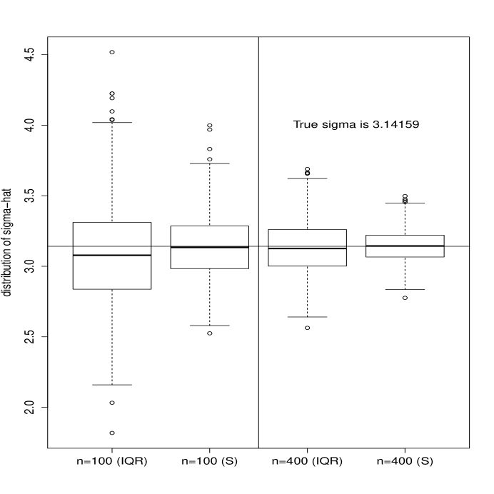
Figure 7: Distribution of sample estimates by estimator and sample size

5.4.1 Solution

1. We know that for a standard normal random variable $P(Z>0.675)=0.25$. So we would expect that the IQR (interquartile range) would extend to $2*.6745=1.35$ standard units. We use this expectation to determine the estimator: $\tilde{s}=IQR/1.35$.

2. We carried out a simple simulation study with a fixed mean and standard deviation (set to $\pi$). A thousand simulations of samples were taken using $\tilde{s}$ and $\hat{s}$ (MLE). The results are displayed in Figure 7. We note that both estimators are less variable when $n=400$ than for $n=100$ and conclude that the variability of the estimators goes down as a function of $\sqrt{n}$.

3. The IQR for $\tilde{s}$ is 0.50 for n=100 and 0.25 for n=400, while the IQR for $\hat{s}$ is 0.30 for n=100 and 0.16 for n=400. We conclude that the MLE is more efficient than our ad-hoc estimator.

5.4.2 Commentary

This exercise was included with a problem set mid-way through the class as the nature and properties of estimators were explored. This problem introduced the idea of a simulation study to investigate the behavior of a new estimator. While the analytic solution was straightforward, it required the students to think about estimation in a different way, and tap properties of the normal distribution. The empirical solution provided a glimpse into the additional variability of the IQR estimator compared to the standard estimator of standard deviation. A full analytic solution for this problem was beyond the scope of the course, but can be undertaken for specific values of $n$.

5.5 Assessing robustness of chi-square statistic to small cell counts

Perform a simulation study on the sensitivity of the $\chi^{2}$ test for the uniform distribution to expected cell counts below 5. Simulate the distribution of the test statistic for 16 and 64 observations from a uniform distribution using 8 equal-length bins (from nola:spee:2000).

simchisq = function(n, bins) {
  vals = cut(runif(n, 0, bins), breaks=0:bins)
  obs = c(table(vals))
  exp = c(rep(n/bins, bins))
  return(sum(((obs - exp)^2)/exp))
}
library(mosaic); par(mfrow=c(1, 2))
bins = 8; n = 16    # Expected count per cell equal to 2
res = do(10000)*simchisq(n, bins)
plot(density(res$result), main="", lwd=2,
     xlab=paste("N=",n,", ",bins," bins", sep=""), xlim=c(0, 20))
curve(dchisq(x, bins-1), 0, max(res$result), add=TRUE, lwd=2, lty=2)

n = 64              # Expected count per cell equal to 8
res = do(10000)*simchisq(n, bins)
plot(density(res$result), main="", lwd=2,
  xlab=paste("N=",n,", ",bins," bins", sep=""), xlim=c(0, 20))
curve(dchisq(x, bins-1), 0, max(res$result), add=TRUE, lwd=2, lty=2)

Figure 8: R code to carry out simulation study (chi-square problem)

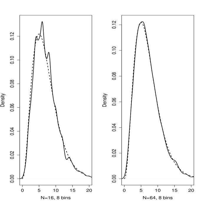
Figure 9: Observed and expected distribution for chi-square statistic

5.5.1 Solution

We know that the chi-square test is recommended only in situations where the expected cell count is 5 or more in each cell. In this simulation study, we generate repeated samples from the null distribution and compare these to the large-sample distribution of the chi-square ($\chi^{2}$) statistic (see Figure 8). We know that in this setting, the appropriate degrees of freedom are equal to the number of bins minus 1. The main work is done using the simchisq() function, which generates data from a continuous uniform variable, then constructs the observed and expected cell counts and the chi-square statistic. This is repeated for the two scenarios and displayed in Figure 9. We see that the observed distribution under the null is somewhat jumpy (due to the discreteness of the possible values) when the expected cell counts are low (left figure), and that the observed curve is quite similar to the chi-square distribution when the expected cell count is 8 (right figure).

5.5.2 Commentary

This problem was intended to provide more practice in the construction of simulation studies as well as introduce new idioms related to looping and writing of functions. It also serves to highlight the importance of assumptions and the idea of sampling under the null distribution (as a precursor to resampling based inference). This was included with a group of problems mid-way through the class as the nature and properties of tests of hypotheses along with sampling distributions under the null were explored.

References

- [1] \harvarditemBarrows \harvardand Tamblyn1980barr:tamb:1980 Barrows, H. \harvardand Tamblyn, R. \harvardyearleft1980\harvardyearright. Problem based learning: an approach to medical education, Springer-Verlag, New York.
- [2] \harvarditemBrown \harvardand Kass2009brow:kass:2009 Brown, E. N. \harvardand Kass, R. E. \harvardyearleft2009\harvardyearright. What is statistics?, The American Statistician 63(2): 105–110.
- [3] \harvarditem[Buttrey et al.]Buttrey, Nolan \harvardand Temple Lang2001butt:nola:2001 Buttrey, S. E., Nolan, D. \harvardand Temple Lang, D. \harvardyearleft2001\harvardyearright. Computing in the mathematical statistics course, ASA Proceedings of the Joint Statistical Meetings .
- [4] \harvarditemCobb2011cobb:2011 Cobb, G. \harvardyearleft2011\harvardyearright. Teaching statistics: some important tensions, Chilean Journal of Statistics 2(1): 31–62.
- [5] \harvarditemCobb1992cobb:1992 Cobb, G. W. \harvardyearleft1992\harvardyearright. Teaching statistics, In Lynn A. Steen (ed), Heeding the call for change: suggestions for curricular action (MAA Notes No. 22) pp. 3–43.
- [6] \harvarditemCohen1992cohe:1992 Cohen, D. W. \harvardyearleft1992\harvardyearright. A modified Moore method for teaching undergraduate mathematics, American Mathematical Monthly 89(7): 473–74,487–490.
- [7] \harvarditem[DelMas et al.]DelMas, Garfield, Ooms \harvardand Chance2006delm:garf:2006 DelMas, R., Garfield, J., Ooms, A. \harvardand Chance, B. \harvardyearleft2006\harvardyearright. Assessing students’ conceptual understanding after a first course in statistics, Proceedings of the Annual Meetings of the American Educational Research Association .
- [8] \harvarditemEvans \harvardand Rosenthal2004evan:rose:2004 Evans, M. J. \harvardand Rosenthal, J. S. \harvardyearleft2004\harvardyearright. Probability and Statistics: the Science of Uncertainty, W H Freeman and Company, New York.
- [9] \harvarditemFroelich2008froe:2008 Froelich, A. \harvardyearleft2008\harvardyearright. Using R in probability and mathematical statistics courses, ASA Proceedings of the Joint Statistical Meetings.
- [10] \harvarditemGAISE College Group2005gaise GAISE College Group \harvardyearleft2005\harvardyearright. Guidelines for assessment and instruction in statistics education, http://www.amstat.org/education/gaise, accessed August 18, 2013, Technical report, American Statistical Association.
- [11] \harvarditem[Gelman et al.]Gelman, Carlin, Stern \harvardand Rubin2004gelm:carl:2004 Gelman, A., Carlin, J. B., Stern, H. S. \harvardand Rubin, D. B. \harvardyearleft2004\harvardyearright. Bayesian data analysis (second edition), Chapman and Hall.
- [12] \harvarditemGentleman \harvardand Temple Lang2007gent:temp:2007 Gentleman, R. \harvardand Temple Lang, D. \harvardyearleft2007\harvardyearright. Statistical analyses and reproducible research, Journal of Computational and Graphical Statistics 16(1): 1–23.
- [13] \harvarditemGould2010goul:2010 Gould, R. \harvardyearleft2010\harvardyearright. Statistics and the modern student, International Statistical Review 78(2): 297–315.
- [14] \harvarditemHalmos1985halm:1985 Halmos, P. \harvardyearleft1985\harvardyearright. I Want to Be a Mathematician: An Automathography, Springer.
- [15] \harvarditem[Horton et al.]Horton, Brown \harvardand Qian2004hort:brow:2004 Horton, N. J., Brown, E. R. \harvardand Qian, L. \harvardyearleft2004\harvardyearright. Use of R as a toolbox for mathematical statistics exploration, The American Statistician 58(4): 343–357.
- [16] \harvarditemIhaka \harvardand Gentleman1996ihak:gent:1996 Ihaka, R. \harvardand Gentleman, R. \harvardyearleft1996\harvardyearright. R: A language for data analysis and graphics, Journal of Computational and Graphical Statistics 5(3): 299–314.
- [17] \harvarditemJones1977jone:1977 Jones, F. B. \harvardyearleft1977\harvardyearright. The Moore method, American Mathematical Monthly 84: 273–278.
- [18] \harvarditemKaplan2003kapl:2003 Kaplan, D. \harvardyearleft2003\harvardyearright. Introduction to Scientific Computation and Programming, CL-Engineering.
- [19] \harvarditemLamport2011latex Lamport, L. \harvardyearleft2011\harvardyearright. LaTeX: a document preparation system, http://www.latex-project.org, accessed August 18, 2013, Technical report, LaTeX Project.
- [20] \harvarditemLavine2013lavi:2007 Lavine, M. \harvardyearleft2013\harvardyearright. Introduction to Statistical Thought, https://www.math.umass.edu/~lavine/Book/book.html, accessed August 18, 2013, Creative Commons.
- [21] \harvarditem[Lazar et al.]Lazar, Reeves \harvardand Franklin2011laza:2011 Lazar, N. A., Reeves, J. \harvardand Franklin, C. \harvardyearleft2011\harvardyearright. A capstone course for undergraduate statistics majors, The American Statistician 65(3): 183–189.
- [22] \harvarditem[Legler et al.]Legler, Roback, Ziegler-Graham, Scott, Lane-Getaz \harvardand Richey2010legl:2010 Legler, J., Roback, P., Ziegler-Graham, K., Scott, J., Lane-Getaz, S. \harvardand Richey, M. \harvardyearleft2010\harvardyearright. A model for an interdisciplinary undergraduate research program, The American Statistician 64: 184–189.
- [23] \harvarditemLeisch2002leis:2002 Leisch, F. \harvardyearleft2002\harvardyearright. Sweave, part I: Mixing R and LaTeX, R News 2(3): 28–31.
- [24] \harvarditemMcLoughlin2008mclo:2008 McLoughlin, P. \harvardyearleft2008\harvardyearright. A modified Moore approach to teaching probability and mathematical statistics: An inquiry based learning technique, ASA Proceedings of the Joint Statistical Meetings.
- [25] \harvarditem[Moore et al.]Moore, Cobb, Garfield \harvardand Meeker1995moor:cobb:1995 Moore, D. S., Cobb, G. W., Garfield, J. \harvardand Meeker, W. Q. \harvardyearleft1995\harvardyearright. Statistics education fin de siècle, The American Statistician 49: 250–260.
- [26] \harvarditemNolan2003nola:2003 Nolan, D. A. \harvardyearleft2003\harvardyearright. Case studies in the mathematical statistics course, Science and statistics: A festschrift for Terry Speed (IMS Press, Fountain Hills, AZ) pp. 165–176.
- [27] \harvarditemNolan \harvardand Speed2000nola:spee:2000 Nolan, D. \harvardand Speed, T. (eds) \harvardyearleft2000\harvardyearright. Stat Labs: Mathematical Statistics Through Applications, Springer-Verlag, New York.
- [28] \harvarditemNolan \harvardand Temple Lang2003nola:temp:2003 Nolan, D. \harvardand Temple Lang, D. \harvardyearleft2003\harvardyearright. Case studies and computing: broadening the scope of statistical education, Proceedings of the 2003 ISI Meeting.
- [29] \harvarditemNolan \harvardand Temple Lang2010nola:temp:2010 Nolan, D. \harvardand Temple Lang, D. \harvardyearleft2010\harvardyearright. Computing in the statistics curriculum, The American Statistician 64(2): 97–107.
- [30] \harvarditemPruim2011prui:2011 Pruim, R. \harvardyearleft2011\harvardyearright. Foundations and Applications of Statistics: An Introduction using R, American Mathematical Society.
-
[31]
\harvarditemR Core Team2013r-ref
R Core Team \harvardyearleft2013\harvardyearright.
R: A Language and Environment for Statistical Computing, R
Foundation for Statistical Computing, Vienna, Austria.
\harvardurlhttp://www.R-project.org/ - [32] \harvarditemRice1995rice:1995 Rice, J. A. \harvardyearleft1995\harvardyearright. Mathematical statistics and data analysis, Duxbury.
- [33] \harvarditemRossman \harvardand Chance2003obsolete Rossman, A. \harvardand Chance, B. \harvardyearleft2003\harvardyearright. Notes from the 2003 JSM session Is the Math Stat Course Obsolete? www.amstat.org/sections/educ/MathStatObsolete.pdf, accessed August 18, 2013, Technical report, American Statistical Association.
- [34] \harvarditem[Smith et al.]Smith, Yoo \harvardand Nichols2009chri:2009 Smith, J. C., Yoo, S. \harvardand Nichols, S. R. \harvardyearleft2009\harvardyearright. Evaluation and assessment: Effectiveness of the method, The Moore Method: A Pathway to Learner-Centered Instruction, pp. 139–149.
- [35] \harvarditem[Wild et al.]Wild, Pfannkuch, Regan \harvardand Horton2010wild:2010 Wild, C. J., Pfannkuch, M., Regan, M. \harvardand Horton, N. J. \harvardyearleft2010\harvardyearright. Towards more accessible conceptions of statistical inference (with discussion), Journal of the Royal Statistical Society, Series A (Applied Statistics) 174: 247–295.
- [36] \harvarditemWorkgroup on Undergraduate Statistics2000asa-undergrad Workgroup on Undergraduate Statistics \harvardyearleft2000\harvardyearright. Guidelines for undergraduate statistics programs, http://www.amstat.org/education/curriculumguidelines.cfm, accessed August 18, 2013, Technical report, American Statistical Association.
-
[37]
\harvarditemXie2012knitr
Xie, Y. \harvardyearleft2012\harvardyearright.
knitr: A general-purpose package for dynamic report generation
in R.
R package version 0.8.
\harvardurlhttp://CRAN.R-project.org/package=knitr, accessed August 18, 2013 - [38]