Critical transitions in a model of a genetic regulatory system

Abstract.

We consider a model for substrate-depletion oscillations in genetic systems, based on a stochastic differential equation with a slowly evolving external signal. We show the existence of critical transitions in the system. We apply two methods to numerically test the synthetic time series generated by the system for early indicators of critical transitions: a detrended fluctuation analysis method, and a novel method based on topological data analysis (persistence diagrams).

Jesse Berwald

Institute for Mathematics and Its Applications

Minneapolis, Minneapolis, MN 55455, USA

Marian Gidea

Yeshiva University, Department of Mathematical Sciences,

New York, NY 10016

and

School of Mathematics, Institute for Advanced Study

Princeton, NJ 08540, USA

(Communicated by the associate editor name)

1. Introduction

Gene expression is the process by which the genetic code is used to synthesize functional gene products (proteins, functional RNAs). The timing and the level of gene production is specified by a wide range of mechanisms, termed gene regulation. It is believed that a significant number of genes express cyclically, with about $10-15$% of genes directly regulated by the circadian molecular clock. Such gene expression oscillations allow for rapid adaptation to changes in intracellular and environmental conditions. In general, the phase and amplitude of gene expression depend on the function of the gene and internal and external stimuli. It has been postulated that gene expression oscillation is a basic property of all genes, not necessarily connected with any specific gene function [27].

Gene regulatory systems are intrinsically stochastic. Stochasticity originates in the statistical uncertainty of the chemical reactions between molecules, and is inversely proportional to the square root of the number of molecules. Thus, lower numbers of interacting molecules yield increasingly significant statistical fluctuations. Besides intrinsic stochasticity, gene expression is also subjected to extrinsic stochasticity, due to environmental effects. In general, stochastic fluctuations are seen as a source of robustness and stability, but sometimes can adversely affect a cell function [22].

A motivation for the modeling and simulation of gene regulatory systems comes from synthetic biology, an emerging field of research devoted to the design and construction of biological systems, based on engineering principles. An interesting analogy in [31] compares a molecular network to an electrical circuit, where, instead of resistors, capacitors and transistors connected via circuits one has genes, proteins, and metabolites connected via chemical reactions and molecular pathways. Some milestone achievements in this direction have been reported, e.g., in [1, 10, 13]. Relatedly, one would also like to achieve a clear understanding of the functionality of the molecular circuits and networks through measurements of various product outputs, in the same way one understands an electrical circuit through measurements of current, voltage, and resistance. In particular, one would like to discern possible ways in which systems subjected to varying parameters and noise may switch between different stable regimes, or more generally, between potential attractors.

It is the concept of suddenly shifts amongst stable regimes which we explore in this paper. We investigate the occurrence of these critical transitions in a model of a genetic regulatory system. By a critical transition we mean a sudden change of a system from one stable regime (fixed point, limit cycle) to an unstable regime, possibly followed by some other stable regime. We consider a simple genetic circuit that exhibits an oscillatory regime, and we study the behavior of the system under noise. Explicitly, we consider a two-gene model whose oscillations depend on several parameters. We show that the system undergoes a critical transition under slow parameter drift. We accomplish this by recording the time series generated by this model and analyzing the critical transitions. We utilize numerical methods to identify early warning signals indicative of critical transitions in the synthetic data.

First, we apply a statistical method, based on detrended fluctuation analysis, to analyze these time series data. The method is described in detail in Subsection 4.1. The tests are performed using a windowed analysis of the data and reveal that the autocorrelation of the time series increases towards $1$, and the variance of the time series distribution grows steadily prior to a critical transition. These signs are consistent with early warning indicators of critical transitions described by others; for instance, see results in Scheffer, et al [28].

Secondly, we apply a method from topological data analysis, based on persistence diagrams, which we describe in more detail in Subsection 4.2. Again, we consider windows of data from the time series. In this case, we consider these windows as strings of data points to which we associate filtrations of Rips complexes and for which we generate associated persistence diagrams to analyze the topology of the data at different resolutions. The persistence diagrams reveal qualitative changes in the topology of the strings of data points prior to the critical transitions: the distribution of data points becomes more widespread and/or asymmetric. While the detrended fluctuation analysis has been previously used for detection of critical transitions, the application of persistence diagrams, a method from topological data analysis, is novel.

We also make a comparison between the two methods. While the detrended fluctuation analysis introduces artificial choices and possible bias (see also [2]), the proposed topological method is inherently robust. Note that both methods can be applied to detect or predict critical transitions in experimental data as well. As such, the results from model testing may serve as benchmarks for testing data measured from real world sources.

2. Background

In this section we briefly describe critical transitions in the context of fast-slow systems. We consider both deterministic and stochastic systems. Then we present a simple genetic regulatory model of the substrate-depletion oscillator type.

2.1. Critical transitions

A fast-slow system of ordinary differential equations is a system of the type

(1) $$x^{\prime} = f(x,y),$$

(2) $$\varepsilon y^{\prime} = g(x,y),$$

where $(x,y)\in\mathbb{R}^{m}\times\mathbb{R}^{n}$, $f:\mathbb{R}^{m+n}\to\mathbb{R}^{m}$, $g:\mathbb{R}^{m+n}\to\mathbb{R}^{n}$ are $C^{r}$-functions with $r\geq 3$, $\varepsilon>0$ is a small parameter, and ${}^{\prime}=\frac{d}{dt}$. One can regard $y$ as a fast variable. Rescaling the time $t=\varepsilon\tau$ yields

(3) $$\dot{x} = \varepsilon f(x,y),$$

(4) $$\dot{y} = g(x,y),$$

where $\,\dot{}=\frac{d}{d\tau}$. The singular limit of (1),(2) when $\varepsilon\to 0$ gives the slow subsystem, and the singular limit of (3),(4) gives the fast subsystem. The critical set is defined as

$$C_{0}=\{(x,y)\,:\,g(x,y)=0\}$$

and consists of equilibrium points for the fast subsystem. If the Jacobian $\frac{\partial g}{\partial y}$ is nonsingular on $C_{0}$, then $C_{0}$ is an $m$-dimensional manifold, and is the graph of a smooth function $y=h_{0}(x)$. The slow subsystem is determined by $x^{\prime}=f(x,h_{0}(x))$ and restricts to $C_{0}$. In the case that all eigenvalues of $\frac{\partial g}{\partial y}$ at a point have non-zero real parts, then the point is normally hyperbolic. The set of normally hyperbolic points forms a normally hyperbolic invariant manifold (NHIM). In particular, it has stable and unstable manifolds. The NHIM can have attractive components, where all the eigenvalues of $\frac{\partial g}{\partial y}$ have negative real part, and repelling components, where at least one eigenvalue has positive real part. An attractive component has an $n$-dimensional stable manifold, while a repelling component has a non-trivial unstable manifold.

Fenichel’s Theorem [11] implies that, for all sufficiently small $\varepsilon$, every compact submanifold (with boundary) $S_{0}$ of $C_{0}$ can be continued to a NHIM $S_{\varepsilon}$ (not uniquely defined) for the flow of (1), (2), which is the graph of a smooth function $y=h_{\varepsilon}(x)$. The stable and unstable manifolds of $S_{0}$ continue to stable and unstable manifolds of $S_{\varepsilon}$. The flow on $S_{\varepsilon}$ converges to the slow flow as $\varepsilon\to 0$. Such a manifold $S_{\varepsilon}$ is referred to as a slow manifold.

We define a critical transition for this type of system following [17]. We assume that the critical set $C_{0}$ can be decomposed as $C_{0}=S^{a}_{0}\cup S^{r}_{0}\cup S^{b}_{0}$, where $S^{a}_{0}$ is an attractive NHIM, $S^{r}_{0}$ a repelling NHIM, and $S^{b}_{0}$ is the part of $C_{0}$ that is not normally hyperbolic (corresponding to bifurcation points). By definition, a point $p_{0}=(x_{0},y_{0})$ on $C_{0}$ that is not normally hyperbolic is a critical transition if there exists a concatenation of trajectories $\gamma_{0}$, $\gamma_{1}$, where $\gamma_{0}:[t_{-1},t_{0}]\to\mathbb{R}^{m+n}$, $\gamma_{1}:[t_{0},t_{1}]\to\mathbb{R}^{m+n}$ satisfy the following properties:

• $\gamma_{0}(t_{-1},t_{0})$ is a trajectory of the slow subsystem, oriented from $\gamma_{0}(t_{-1})$ to $\gamma_{0}(t_{0})$, contained in the attracting NHIM $S^{a}_{0}$;

• $\gamma_{0}(t_{0})=\gamma_{1}(t_{0})=p_{0}\in S^{b}_{0}$ is a point that is not normally hyperbolic;

• $\gamma_{1}(t_{0},t_{1})$ is a trajectory of the fast subsystem, oriented from $\gamma_{1}(t_{0})$ to $\gamma_{1}(t_{1})$.

When we consider the dynamics of the system for $\varepsilon>0$ sufficiently small, a trajectory starting near $\gamma_{0}$ follows closely the slow dynamics around $\gamma_{0}$ for some time, after which it transitions to follow the fast dynamics near $\gamma_{1}$ for a period of time. In [17, 18] several types of bifurcations are examined to determine whether or not they exhibit the characteristics of critical transitions, under some suitable conditions on the smoothness, compactness, and non-degeneracy on the system. We summarize the findings below:

• for $m=n=1$, saddle-node (fold) bifurcation points determine critical transitions;

• for $m=n=1$, subcritical pitchfork bifurcation points determine critical transitions;

• for $m=n=1$, transcritical bifurcation points determine critical transitions;

• for $m=2$ and $n=1$, subcritical non-degenerate Hopf bifurcations determine critical transitions.

2.2. Incorporating noise

It is often important for the understanding of a physical system to incorporate stochastic effects. We consider the Langevin form of (1), (2)

(5) $$dx = f(x,y)+\sigma_{1}dW_{1},$$

(6) $$dy = \frac{1}{\varepsilon}g(x,y)+\frac{1}{\sqrt{\varepsilon}}\sigma_{2}dW_{2},$$

where $\sigma_{1}$, $\sigma_{2}$ represent noise levels (depending on $\varepsilon$), and $W_{1},W_{2}$ are one-dimensional Wiener processes (Brownian motions). Assuming $\sigma_{1},\sigma_{2}$ are sufficiently small, the sample paths of the system (5), (6) stay near $S^{a}_{0}$ with high probability, up to a neighborhood of the critical transition, after which they exit the neighborhood. In [17, 18], it is argued that the following behaviors are typical of a system prior to a critical transition:

• The system recovery from small perturbations is ‘critically’ slows down;

• The variance in the time series increases steadily;

• The autocorrelation of the time series increases towards $1$;

• The distribution of the time series becomes more asymmetric.

We note that (iv) from above depends on whether or not the underlying bifurcation has symmetry. For example, a saddle-node bifurcation as in (a) from above will typically yield asymmetric fluctuations, while a pitchfork bifurcation as in (b) from above will typically yield symmetric fluctuations. A complementary characteristic to (iv) is that the distribution of the time series loses its normality, for example it changes from uni-modal to multi-modal.

Such system response characteristics can be monitored numerically and serve as ‘early warnings’ of critical transitions in real-world systems. Examples include Earth’s climate, ecological systems, global finance, asthma attacks or epileptic seizures; see, e.g., [7, 28, 29, 30], and the references therein.

2.3. A simple genetic circuit

We briefly describe a model of simple genetic circuit which generates oscillations of varying amplitude. The model consists of two genes, one producing the protein $R(t)$, and the other producing the protein $X(t)$. The protein $X(t)$ is a substrate for the activator protein $R(t)$ that is produced in an autocatalytic process. As $R(t)$ accumulates, the production of $R(t)$ accelerates until there is an explosive conversion of the whole of $X(t)$ into $R(t)$. This rapid change corresponds to a critical transition in the underlying system. With the substrate $X(t)$ depleted, the autocatalytic reaction terminates, and the activator $R(t)$ degrades in time. This allows the level of $X(t)$ to grow again, leading to another cycle of explosive growth in $R(t)$. This process is know as a substrate-depletion oscillator.

An example of this mechanism is the oscillation of the M-phase-promoting factor (MPF) activator in the frog egg, where the substrate is the phosphorylated form of the B-cyclin-dependent kinase (note that the true mechanism involves several other proteins and reactions) [26]. A mathematical model for the substrate-depletion oscillator is given by the following system:

(7) $$X^{\prime}(t) = k_{1}S-[k_{0}^{\prime}+k_{0}E_{P}(R(t))]X(t),$$

(8) $$R^{\prime}(t) = [k_{0}^{\prime}+k_{0}E_{P}(R(t))]X(t)-k_{2}R(t).$$

Here $E_{P}(R(t))$ represents the level of the phosphorylated version of the protein $R(t)$ – involved with $R(t)$ in a mutual activation process – given by $E_{P}(R)=G(k_{3}R,k_{4},J,K)$, where $G$, the Goldbeter-Koshland function, is defined by

$$G(u,v,J,K)=\frac{2uK}{v-u+vJ+uK+\sqrt{(v-u+vJ+uK)^{2}-4(v-u)uK}}.$$

The Goldbeter-Koshland function represents the equilibrium concentration of the phosphorylated form of a protein, for a phosphorylation-dephosphorylation reaction governed by Michelis-Menten kinetics. The Goldbeter-Koshland function is responsible for creating a switch-like signal-response in the evolution of the protein $R(t)$. The quantities $k_{0},k^{\prime}_{0},k_{1},k_{2},k_{3},k_{4},J,K,S$ are parameters. The parameter $S$ is the strength of a signal, representing the rate of synthesis of the substrate $X$, which we regard as an external input to the system.

This system presents both positive and negative feedback. The positive feedback loop creates a bistable system and the negative-feedback loop drives the system back and forth between two stable steady states. In what follows, we will modify the simple genetic circuit in (7) and (8) by considering the external input $S$ as a slowly varying parameter, in addition to including a stochastic term. We will study critical transitions in the resulting system.

3. Model

We consider a new model of a genetic regulatory network with a slowly dependent signal, given by (7), (8), with $S$ being now a slowly evolving parameter, i.e.

(9) $$X^{\prime}(t) = k_{1}S(t)-[k_{0}^{\prime}+k_{0}E_{P}(R(t))]X(t),$$

(10) $$R^{\prime}(t) = [k_{0}^{\prime}+k_{0}E_{P}(R(t))]X(t)-k_{2}R(t),$$

(11) $$S^{\prime}(t) = \varepsilon,$$

where $\varepsilon>0$ is small. We will fix the parameter as in [31], $k_{0}=0.04,k^{\prime}_{0}=0.01,k_{1}=k_{2}=k_{3}=1,k_{4}=0.3,J=K=0.05$.

The fast subsystem is obtained by letting $\varepsilon\to 0$ yielding

(12) $$X^{\prime}(t) = k_{1}S(t)-[k_{0}^{\prime}+k_{0}E_{P}(R(t))]X(t),$$

(13) $$R^{\prime}(t) = [k_{0}^{\prime}+k_{0}E_{P}(R(t))]X(t)-k_{2}R(t),$$

(14) $$S^{\prime}(t) = 0.$$

We rescale time $\tau=\varepsilon t$, and we rewrite the corresponding system relative to the rescaled time

(15) $$\varepsilon\dot{X} = k_{1}S-[k_{0}^{\prime}+k_{0}E_{P}(R)]X,$$

(16) $$\varepsilon\dot{R} = [k_{0}^{\prime}+k_{0}E_{P}(R)]X-k_{2}R,$$

(17) $$\dot{S} = 1.$$

Sample trajectories for this system are plotted in Fig. 1. From the above equations the slow subsystem is obtained by letting $\varepsilon\to 0$ yielding

(18) $$0 = k_{1}S-[k_{0}^{\prime}+k_{0}E_{P}(R)]X,$$

(19) $$0 = [k_{0}^{\prime}+k_{0}E_{P}(R)]X-k_{2}R,$$

(20) $$\dot{S} = 1.$$

From this we see that the critical submanifold is given by

$$C_{0}=\left\{(X,R,S)\,,\,X=\frac{k_{1}S}{k_{0}^{\prime}+k_{0}E_{P}({\frac{k_{1}}{k_{2}}S)}},R=\frac{k_{1}}{k_{2}}S\right\}.$$

The critical submanifold consists of equilibrium points of the fast subsystem. The stability of the $C_{0}$ is determined by the eigenvalues of the Jacobi matrix evaluated at the equilibrium points

$$J=\left(\begin{array}[]{cc}-[k^{\prime}_{0}+k_{0}E_{P}(R)]&-[k_{0}\partial_{R}E_{P}(R)X]\\ k^{\prime}_{0}+k_{0}E_{P}(R)&k_{0}\partial_{R}E_{P}(R)X-k_{2}\\ \end{array}\right).$$

For the values of the parameters chosen above, we find that the stability at an equilibrium point changes at $S_{crit1}=0.13326703$ and $S_{crit2}=0.34680193$, respectively. The corresponding equilibria are $X_{crit1}=5.41285587$, $R_{crit1}=0.13326703$, and $X_{crit2}=1.07370450$, $R_{crit2}=0.34680193$.

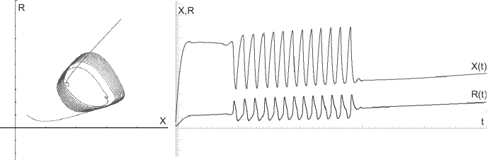
Figure 1. A sample trajectory, and the $X$-time series (higher value) and $R$-time series (lower values).

Precisely, for $S<S_{crit1}$ and $S>S_{crit2}$ the equilibrium point is stable. For $S\in(S_{crit1},S_{crit2})$ the equilibrium point is unstable, and there exists a periodic orbit that is asymptotically stable, whose existence can be established numerically, as observed in Fig. 1. The values $S=S_{crit1}$, $S=S_{crit2}$ yield subcritical Hopf bifurcations, where an unstable equilibrium point is turned into a stable one and a small unstable periodic orbit is born (or vice versa). In addition, one expects canard-type solutions in some exponentially small neighborhoods of $S_{crit1}$, $S_{crit2}$, relative to $\varepsilon$ (see, e.g., [19]). In Fig. 2 we plot the nullclines of the system for the critical points $S_{crit1}$ and $S_{crit2}$.

$$\begin{array}[]{cc}\includegraphics[width=180.67499pt,clip,keepaspectratio]{nullclines01_v2-eps-converted-to.pdf}&\includegraphics[width=180.67499pt,clip,keepaspectratio]{nullclines02_v2-eps-converted-to.pdf}\end{array}$$

Figure 2. The nullclines of the fast system for $S=S_{crit1}$ and $S=S_{crit2}$.

The specific stochastic differential equation (SDE) system associated to (15), (16), (17) can be written

(21) $$\dot{X} = \frac{1}{\varepsilon}(k_{1}S-[k_{0}^{\prime}+k_{0}E_{P}(R)]X)+\frac{\sigma_{1}}{\sqrt{\varepsilon}}dW_{1},$$

(22) $$\dot{R} = \frac{1}{\varepsilon}([k_{0}^{\prime}+k_{0}E_{P}(R)]X-k_{2}R)+\frac{\sigma_{2}}{\sqrt{\varepsilon}}dW_{2},$$

(23) $$\dot{S} = 1,$$

where $W_{1},W_{2}$ represent Brownian motions, and $\sigma_{1},\sigma_{2}$ are noise levels. Since the parameter values $S_{crit1}$ and $S_{crit2}$ yield subcritical Hopf bifurcations, the theory from Subsection 2.1 allows us to conclude that the corresponding points $(X_{crit1},R_{crit1})$, $(X_{crit2},R_{crit2})$ determine critical transitions. A typical trajectory of the stochastic system in the phase space and its corresponding $R$-time series are shown in Fig. 3. Examining the $R$-time series, one can see that a critical transition occurs near time $t\approx 1000$. We note that a similar analysis for activator-inhibitor oscillations has been performed in [18].

Remark 1.

As mentioned in Section 1, noise in the form of random fluctuations arises naturally in gene regulatory networks. One typically distinguishes between intrinsic noise, inherent in the biochemical reactions, and extrinsic noise, originating in the random variation of the externally set control parameters. Both types of noise can be model by augmenting the governing rate equations with additive or multiplicative stochastic terms. We refer the interested reader to [14].

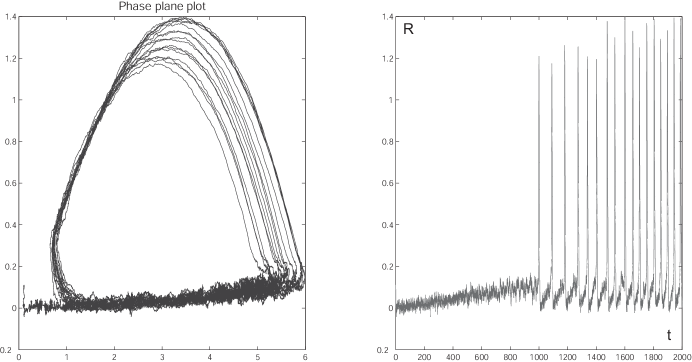
Figure 3. Phase space of the model described by (21), (22), (23), and a corresponding $R$-time series.

In our model we only consider the effects of additive noise, which can be thought of as a randomly varying external field acting on the biochemical reactions. The field enters into the governing rate equations as an additive stochastic term in the Langevin equation. We choose to focus on additive extrinsic noise as this could be used as a switch and/or amplifier for gene expression, which has potential applications to gene therapy [14]. Switching mechanisms are exactly the type of phenomena that we would like to capture via the critical transitions approach.

4. Methods

We use the model proposed in Section 3 to generate a synthetic time series given by successive reading of one of the variables. We investigate the synthetic time series for early warning signs of critical transitions. Below we describe two such detection methods: a well-known detrended fluctuation analysis method, and a novel method inspired by topological data analysis.

4.1. Detrended fluctuation analysis

Detrended fluctuation analysis (DFA) is a technique introduced by Hurst half a century ago to analyze fluctuations in time series. The DFA procedure has been widely used for early detection of critical transitions [23, 28, 30]. We outline the algorithm below.

4.1.1. Algorithmic description of DFA

The DFA procedure takes as input a time series $(s_{k},z_{k}),\,k=1,\ldots,N$, where $s_{k}$ is the instant of time of the $k$-th measurement (not necessarily equally spaced), and $z_{k}$ is the $k$-th measurement of some observable. To detect whether the system undergoes a critical transition, the DFA algorithms proceeds as follows:

Interpolation:

Choose an optimal step size $\Delta t$, and interpolate the given time series such that it is evenly spaced in time. Denote the new series $(t_{k},x_{k})$, with $t_{k}=k\Delta t$.

Detrending:

One way to remove a general trend from statistical data is by subtracting a moving average. For example, using a Gaussian kernel

$$G_{k}(t)=\frac{1}{\sqrt{2\pi}d}\exp\left(-\frac{(t-k\Delta t)^{2}}{2d^{2}}\right)$$

of bandwidth $d$, one may compute the weighted average of $x_{k}$,

$$X(k\Delta t)=\frac{\sum_{i=1}^{N}G_{k}(i\Delta t)x_{i}}{\sum_{i=1}^{N}G_{k}(i\Delta t)}.$$

Subtracting the weighted average from the time series yields the detrended series,

$$y_{k}=x_{k}-X(k\Delta t)$$

.

Remark 2.

Instead of Gaussian kernel detrending, alternative detrending methods can be used, such as linear, cubic spline, or Fourier interpolation, depending on the nature of the data. We also explore these additional methods in Section 5

Lag-1 autocorrelation:

The final step involves fitting a first-order autoregressive (AR(1)) process

$$y_{k+1}=c_{k}y_{k}+\sigma\xi_{k},$$

to the detrended time series $y_{k}$, where $(\sigma\xi_{k})_{k\in\mathbb{N}}$ is white noise of intensity $\sigma$. In order to compute $c_{k}$, choose a sliding window of size $w$ and determine the least-squares fit

$$y_{j+1}\approx c_{k}y_{j},\quad\textrm{ for }j=k,\ldots,k+w-1.$$

Hence, for each window we extract the value of $AR(1)$ $c_{k}$. Recall that the lag-1 autocorrelation $AR(1)$ is $0$ for white noise and close to $1$ for red (autocorrelated) noise.

4.1.2. Detection of critical transitions via DFA

The following criterion has been proposed for the detection of critical transition [28]:

• Given a time series measured from a system approaching a critical transition, the DFA outputs a time series $(t_{k},y_{k})$ for which

  1. the autocorrelation has a general trend which increases towards $1$;

  2. the variance has a positive trend.

In certain special cases, this criterion has a rigorous justification [17, 18].

The DFA method is an effective tool in detecting early signs of critical transitions in noisy data. However, the method comes with several significant drawbacks, such as its sensitivity to the procedures and parameters used in processing the data. For instance, the sample frequency, detrending method (e.g., the bandwidth of the Gaussian detrending), or the size of the sliding window all have a strong effect on the conclusions drawn from the algorithm in subsection 4.1 and hence on the power of the DFA method to serve as a prediction tool. One concern is that the measurement of the $AR(1)$ values as well as the variance are strongly influenced by the fit of the detrending method, with a poor fit being likely to signal ‘false positives’ for critical transitions (see [2]).

4.2. Persistence diagrams

As mentioned in Section 1, we propose to use tools from the field of topological data analysis as a new method to detect critical transitions in dynamical systems. In particular, we leverage the stability properties of persistence diagrams to detect critical transitions. Topological persistence is a relatively recent development that forms the core of topological data analysis and has been widely used to extract relevant information from noisy data (see [8] for background in persistence topology in general). There are numerous applications, including computer vision, cluster analysis, biological networks, cancer survival analysis, and granular material (see [4, 8, 12, 20, 25] and the references listed there).

In this section we describe the way in which we adapt this method to observe changes in time series from systems approaching or undergoing critical transitions. The key idea is to extract from the time series consecutive strings of data points of a fixed length, which we regard as individual point cloud data sets. To each such point cloud we assign a topological invariant, namely its persistence diagram. Roughly speaking, the persistence diagram is a representation of the data set in an abstract metric space which encodes information about topological features of the data.

The highlight of this method is that when the system undergoes a critical transition, the topological features associated to the point cloud data sets also change significantly. The fact that the corresponding persistence diagrams and distances between them can be computed algorithmically enables us to describe these changes quantitatively.

4.2.1. Description of persistence diagrams

We describe the concept of a persistence diagram associated with point cloud data starting with an informal description. From a high-level perspective, the data analysis pipeline works as follows:

$$\text{Data }\implies\text{ Filtration }\implies\text{ Persistence Module }\implies\text{ Persistence Diagram}$$

We focus on the first two and the fourth parts of this pipeline, and only briefly detail the algebraic aspects of the third component below. Suppose that one is provided with a point cloud data set, $X_{0}$, that is an approximation of some geometric shape. One would like to infer from the data the topological information on that shape. However, a finite collection of points has only trivial topology. One way to convert the collection of points into a non-trivial topological space is to replace the points of the set by balls of a certain radius $\epsilon$. One then computes the topological features of the resulting set, $X_{\epsilon}$. Typical invariants resulting from this computation, which serve to classify the set, include the number connected components along with the number of ‘tunnels’ and number of ‘cavities’ (known as Betti numbers).

Of course, the topology of $X_{\epsilon}$ depends on the choice of the radius of the balls in this construction. Instead of fixing a certain radius, topological persistence considers all possible radii, from some sufficiently small value, up to a sufficiently large radius. This growth of the radius yields the filtration step above. As the radius is gradually increased, new topological features will be ‘born’ and certain existing ones will ‘die’. A schematic representation of this process is depicted in Fig. 4. The birth and death of each topological feature at a given dimension is recorded by a persistence diagram. This is a collection (multiset actually) of (birth,death) times in $\mathbb{R}^{2}$. The 0- and 1-dimensional diagrams for the associated filtration are shown in the bottom row of Fig. 4.

The lifespan of a feature is easily computed by calculating (death time) - (birth time). A topological feature with a long lifespan, measured by the range of radii over which it ‘persists’, is likely to capture an essential topological feature of the underlying space from which the data was sampled. On the other hand, short lived features are likely to result from ‘noise’ in the data. However, rather than discriminating between what is an essential feature of the topology and what is not, the persistence diagram method provides a summary of topological features that appear and disappear throughout the variation of the radii of the balls, as well as a ranking of the significance of these features, expressed in terms of the lifespans.

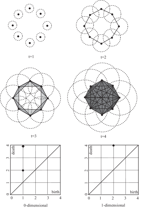
Figure 4. A collection of points in the plane, resembling a ‘noisy’ circle, is given. At each instant of time $t=1,\ldots,4$, around each point we constructs disks of radii $\delta_{1}/2,\ldots,\delta_{4}/2$, respectively, with $\delta_{1}<\delta_{2}<\delta_{3}<\delta_{4}$. The corresponding Rips complexes are also constructed at each instant. The topological features of the Rips complexes change as time increases. At time $t=1$ there are 8 connected components and no 1-dimensional hole. At time $t=2$ the connected components coalesce into a single component (thus in the 0-dimensional diagram there are actually 7 deaths represented at $(1,2)$), and a 1-dimensional hole is born. Both the single connected component and the 1-dimensional hole survive to $t=3$. At time $t=4$ the 1-dimensional hole dies as it fills in (the death is represented at $(2,4)$), while the single connected component continues living (in fact, it has infinite lifespan). The $\Diamond$ at $(1,4)$ represents this fact.

We now continue with a concise, formal description of persistence diagrams. For an introduction to algebraic topology and homology, see [15]; surveys of persistent topology can be found in [8, 32] Given point cloud data $X\subset\mathbb{R}^{d}$, i.e., a collection of points in $\mathbb{R}^{d}$, and $\delta>0$, we associate to them the Rips complex $\mathcal{R}_{\delta}$. This is, by definition, the abstract simplicial complex whose $0$-simplices are points $x_{\alpha}$, and whose $k$-simplices are given by unordered $(k+1)$-tuples of points $\{x_{\alpha_{j}}\}_{j=0,\ldots,k}$ which are pairwise within a distance $\delta$. Figure 4 provides an example for $X\subset\mathbb{R}^{2}$. For all $0<a<b$ we have $\mathcal{R}_{a}\subset\mathcal{R}_{b}$. That is, the family $\{\mathcal{R}_{\delta}\}_{\delta>0}$ forms a filtration.

Denote by $H_{p}(\mathcal{R}_{a})$ the $p$-homology of $\mathcal{R}_{a}$ with $\mathbb{Z}_{2}$ coefficients. Heuristically, the homology of a simplicial complex provides information about the topological features of the complex, e.g., the number of connected components, tunnels and cavities in that complex. The inclusion $\mathcal{R}_{a}\hookrightarrow\mathcal{R}_{b}$ induces the homomorphisms $f^{a,b}_{*}:H_{*}(\mathcal{R}_{a})\to H_{*}(\mathcal{R}_{b})$ in all dimensions. Note that the image $F^{a-\rho,b}$ of $f^{a-\delta,a}_{*}$ in $H_{*}(\mathcal{R}_{b})$ is independent of $\rho$ for all $\rho>0$ sufficiently small. We denote this image by $F^{a-,b}_{*}$.

A real value $c>0$ is called a homological critical value if there exists $q$ such that the homomorphism $f^{c-\rho,c}_{q}:H_{q}(\mathcal{R}_{c-\rho})\to H_{q}(\mathcal{R}_{c})$ is not an isomorphism for all sufficiently small $\rho>0$. The image $F_{q}^{c-,c}$ of $f^{c-\rho,c}_{q}$ in $H_{q}(\mathcal{R}_{c})$ is independent of $\rho$, if this is small enough. The quotient group $B_{q}^{c}=H_{q}(\mathcal{R}_{c})/F_{q}^{c-,c}$ is called the $q$-th birth group at $\mathcal{R}_{c}$, and it captures the homology classes that did not exist in $\mathcal{R}_{c-\rho}$. A homology class $\alpha\in H_{q}(\mathcal{R}_{c})$ is born in $\mathcal{R}_{c}$ if it represents a non-trivial element in $B_{q}^{c}$, that is, the canonical projection of $\alpha$ is non-zero.

Now consider the homomorphism $g^{a,b}_{q}:B_{q}^{a}\to H_{q}(\mathcal{R}_{b})/F^{a-,b}$, where $g^{a,b}_{q}([\alpha])=[f^{a,b}_{q}(\alpha)]$, for $\alpha\in H_{q}(\mathcal{R}_{b})$, where the notation $[\cdot]$ stands for equivalence class. We set $g_{q}^{a,b}=0$ for all $b>0$ sufficiently large. The kernel $D_{q}^{a,b}$ of the map $g^{a,b}_{q}$ is called the death subgroup of $B_{q}^{a}$ at $\mathcal{R}_{q}^{b}$. A homology class $\alpha\in H_{q}(\mathcal{R}_{a})$ dies entering $\mathcal{R}_{b}$ if $[\alpha]\in D_{q}^{a,b}$ but $[\alpha]\not\in D_{q}^{a,b-\rho}$, for $\rho>0$ sufficiently small. The degree $r$ of the death value $b$ of $B^{a}_{q}$ is defined by $r=\textrm{rank}D_{q}^{a,b}-\textrm{rank}D_{q}^{a,b-}$. The sum of the degrees of all death value of the birth group $B_{q}^{a}$ is clearly equal to $\textrm{rank}(B^{a}_{q})$. The birth time of a homology class $\alpha$ is the value $a>0$ where the $\alpha$ is born in $\mathcal{R}_{a}$, and the death time is the value $b>0$ where $\alpha$ dies in $\mathcal{R}_{b}$.

The $q$-persistence diagram of the filtration $(\mathcal{R}_{\delta})_{\delta>0}$ is defined as a multiset $\mathcal{P}_{q}$ in $\mathbb{R}^{2}$ consisting of points of the type $z_{i}=(a,b_{i})$, where $a$ is a birth value corresponding to a non-trivial group $B_{p}^{a}$, and $b_{i}$ is a death value of $B_{p}^{a}$; the point $z_{i}$ appears in the diagram with multiplicity equal to the degree $r_{i}$ of the death value $b_{i}$. Since deaths occur after births, all points $(a,b_{i})$ lie above the diagonal set of $\mathbb{R}^{2}$. By default, the diagonal set of $\mathbb{R}^{2}$ is part of the persistence diagram, representing all trivial homology generators that are born and die at every level. Each point on the diagonal has infinite multiplicity. The axes of the persistence diagram are birth values on the horizontal axis and death values on the vertical axis. Again, see Figure 4 for a schematic representation of the construction of a persistence diagram.

It is convenient to define a metric on the space of persistence diagrams. A number of options exist. A fairly standard metric is the $p$-Wasserstein metric. On the set of the $q$-persistence diagrams consider the $p$-Wasserstein metric, $1\leq p\leq\infty$, defined by

$$d_{p}(\mathcal{P}^{1}_{q},\mathcal{P}^{2}_{q})=\left(\inf_{\phi}\sum_{z\in\mathcal{P}^{1}_{q}}\|z-\phi(z)\|_{\infty}^{p}\right)^{1/p},$$

where $\mathcal{P}^{1}_{q},\mathcal{P}^{2}_{q}$ are two $q$-persistence diagrams, and the sum is taken over all bijections $\phi:\mathcal{P}_{q}^{1}\rightarrow\mathcal{P}^{2}_{q}$. The set of bijections, $\{\phi:\mathcal{P}^{1}_{q}\to\mathcal{P}^{2}_{q}\}$, is nonempty owing to the fact that each diagram includes the diagonal set, allowing one to match off-diagonal elements in one diagram with diagonal elements in another when their numbers differ.

The space of $q$-persistence diagrams together with the $p$-Wasserstein metric forms a metric space, which is complete and separable. The Wasserstein distance takes the ‘best’ matching; that is, it minimizes the distance, relative to the $L_{p}$ norm, that one has to shift generators in $\mathcal{P}^{1}_{q}$ to match them with those in $\mathcal{P}^{2}_{q}$. In probability theory, and in particular cases with continuous or weighted distributions, the Wasserstein metric is sometimes termed the ‘earth mover distance’, which refers to the operation of transforming one distribution into another with the minimal change in mass. In what follows we set $p=2$ and drop the reference to $p$. For details on the Wasserstein metric, see [6].

One of the remarkable properties of persistence diagrams is their stability, meaning that small changes in the initial point cloud data produce persistence diagrams that are close to one another relative to Wasserstein metric. The stability results are very general for the ‘bottleneck distance’, when $p=\infty$, and more restrictive for the Wasserstein metric with $p<\infty$. The essence of the stability results, as shown in [3, 6, 9], is that the persistence diagrams depend Lipschitz-continuously on point cloud data.

In applications, the stability result ensures the robustness of the data analysis performed via persistence diagrams, which makes them a powerful alternative to statistical methods. This is particularly useful in context of data from stochastic systems, since persistence diagrams turn out to be quite versatile in distinguishing between small but relevant features in a data set and noise.

4.2.2. Detection of critical transitions via persistence diagrams

We now describe how to apply this method to detect critical transitions in time series. Consider a time series $(t_{j},x_{j})$, $j=1,\ldots,J$, with $x_{j}\in\mathbb{R}^{d}$. (In the case of a time series obtained from the model discussed in Section 3, we will chose $d=1$). Assume that the time series $(t_{j},x_{j})$ is obtained as a time discretization of a process $(t,x_{t})$ which is Lipschitz continuous. (This is indeed the case when a time series is obtained from a Langevin equation, as in Subsection 3.) To each $t_{i}$ we associate a string of $N$ consecutive data points points from the time series, with $N$ sufficiently large, which we denote

(24) $$t_{i}\mapsto X_{i}=(x_{i},x_{i+1},\ldots,x_{i+N-1}).$$

We regard each $X_{i}$ as a point cloud set in $\mathbb{R}^{d}$. We compute the persistence diagrams $\mathcal{P}_{*}(X_{i})$ of $X_{i}$, in all dimensions, and follow the evolution of the persistence diagrams in time.

Diagrams corresponding to nearby times will be close to one another, due to the Lipschitz continuity of the process underlying the time series and to the robustness of persistence diagrams. Within this context, persistence diagrams that are near to each other in time, but relatively far from one another in the Wasserstein metric, indicate a sudden change in the time series. Therefore, we propose the following empirical criterion for detection of critical transitions in slow-fast systems:

• Persistence diagrams undergo significant changes, measured using the Wasserstein metric, prior to a critical transition.

This criterion follows from the following heuristic argument. If the noise level in the Langevin equation is small, then far from a critical transition the time series follows closely, with high probability, a trajectory of the slow subsystem. A point cloud associated to a data string displays significant topological features similar to those of the slow manifold, plus less significant topological features due to noise. In addition, the corresponding persistence diagrams at nearby times are close to one another relative to the Wasserstein metric.

When the system undergoes a critical transition, the time series ceases to follow the slow manifold, as the dynamics enters a transient regime. The topological features associated to the slow manifold are destroyed, and new topological features appear in the point cloud structure. Furthermore, if the system moves to a different stable regime after a finite time, the point cloud will reflect the topological features associated to that regime. Critically, for a point cloud data near a critical transition the corresponding persistence diagrams shift away from those diagrams corresponding to data far from the critical transition. Consequently, successive distances between diagrams in this region exhibit a large jump prior to a critical transition.

5. Results

We numerically solve the SDE defined in (21) – (23) using the Euler-Maruyama procedure, with stepsize $0.01$ and noise level $\sigma_{1}=\sigma_{2}=0.02$. We fix the rate of change of the parameter $S$ to be $\varepsilon=10^{-4}$. As output, we choose the time series given by the $R$-component; a particular realization of this time series is shown in the righthand panel of Fig. 3. Since the solution values are dense in time, we subsample the time series by taking every $10$-th data point. The time series follows a slowly varying attractive equilibrium point, until it reaches a critical transition, at which point it enters an oscillatory mode. To test for early signs of the critical transition, we truncate the time series before it enters the oscillatory regime. This truncated region is shown in Fig. 5.

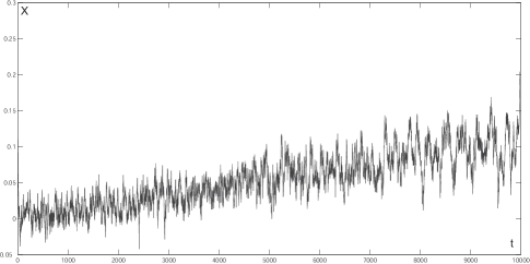
Figure 5. $R$-time series for the gene regulatory network model from Section 3 cut off before the critical transition.

5.1. DFA analysis

We conduct three experiments to detect critical transitions using the DFA methodology on the time series generated by our model. The first experiment uses a Gaussian kernel to detrend the time series; in the second experiment we use a cubic spline interpolation; and in the third experiment, we use Fourier interpolation. For each of the detrended time series we compute $AR(1)$ and the variance for a windowed time series. The results are summarized in Fig. 6. All three experiments show $AR(1)$ increases to $1$ as the system approaches the transition, while the variance also grows steadily, both behaviors being consistent with a critical transition.

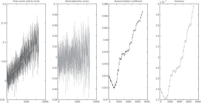
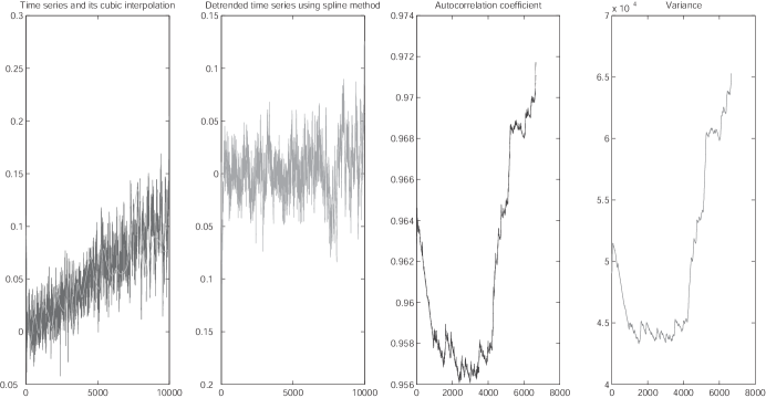
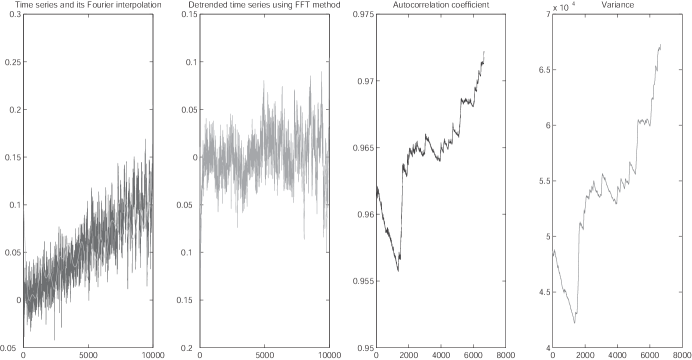
Figure 6. DFA analysis of the time series using (top to bottom) Gaussian kernel, cubic spline, and Fourier interpolation detrending.

5.2. Persistence diagram analysis

We compute the $0$-dimensional persistence diagrams for strings of $N$ data points $X_{i}$ (see Eq. (24)) as the $t_{i}$ approaches a critical transition, as for the example time series in Fig. 5. We construct Rips complexes, with an initial radius of $\delta=10^{-4}$ around each data point, and then grow the radii of the balls $\delta,2\delta,\ldots,n\delta$, where $n$ is chosen large enough so that the final complex in the resulting filtration has a single connected component. From this filtration we compute the $0$-persistence diagrams. We choose the size of the data sets $N=300$; larger sizes make little difference in the qualitative behavior of the diagrams.

The $0$-dimensional persistence diagrams are easy to interpret: they track of the births and deaths of connected components in the Rips complex, as the radii of the balls increase. Note that all births occur at the same time, when the radius of balls is zero and we have $N$ disjoint points. After this initial stage, a large number of connected components die as the radii of the balls increase, as connected components merge with one another.

$\begin{array}[]{cc}\includegraphics[width=162.60638pt,clip,keepaspectratio]{sd4070-0-eps-converted-to.pdf}&\includegraphics[width=162.60638pt,clip,keepaspectratio]{sd9680-0-eps-converted-to.pdf}\end{array}$

Figure 7. The 0-persistence diagram on the left corresponds to a string of data sampled far from the critical transition; the diagram on the right corresponds to a string of data sampled near the critical transition. In each persistence diagram, the dots mark finite deaths times, and the diamond indicates infinite death times.

Consider Fig. 7, where the persistence diagrams for a data string far from the critical transition (left panel) and a data string close to the critical transition (right panel) are shown. For data far from the critical transition, points cluster near the attractive equilibrium. Thus, when balls are constructed in the Rips filtration around these points, they will quickly yield a robust connected component around the attractive equilibrium , plus a small number of scattered connected components corresponding to points that escape for brief periods time from the equilibrium point due to stochastic effects. The implication is that, in the corresponding persistence diagram, the vertical spread of the death times is relatively small, and consists of a small numbers of points away from the diagonal (accounting for the robust connected component and a few outliers), plus many short-lived points close to the diagonal (accounting for noise).

Conversely, when a data string originates from close to a critical transition, the points tend to spread further away from the attractive equilibrium point, due to changes in the potential field. Heuristically, the equilibrium loses its attractiveness. This causes the distribution of the data points from the time series to grow. The implication is that, in the corresponding persistence diagram, the vertical spread of the death times is much larger, with a tendency to form multiple small clusters.

The visual inspection of persistence diagrams provides intuition, but is not a precise way to indicate the approach to a critical transition. To quantify the above assessment, we study the behavior of the Wasserstein distances between consecutive diagrams which are summarized in Fig. 8. In the figure, time increases from left to right. The figures in the top row represent persistence diagrams for data sampled far from the critical transition, and those in the middle represent persistence diagrams for data sampled close to the critical transition. The five time frames captured in each column spread over a time interval of size $\Delta t=0.5$. We then compute the Wasserstein distances between consecutive persistence diagrams. These changes in the persistence diagrams are quantified in the bottom row of Fig. 8. The solid curve, corresponding to data near the critical transition, shows a significant increase in the distances between consecutive diagrams as the point cloud anayzed near the critical transition. The dotted curve, corresponding to distances between diagrams far from the critical transition, shows only small variations in the consecutive distances. The computed distance are indicated by the symbols on each curve and are placed between the diagrams from which they were computed.

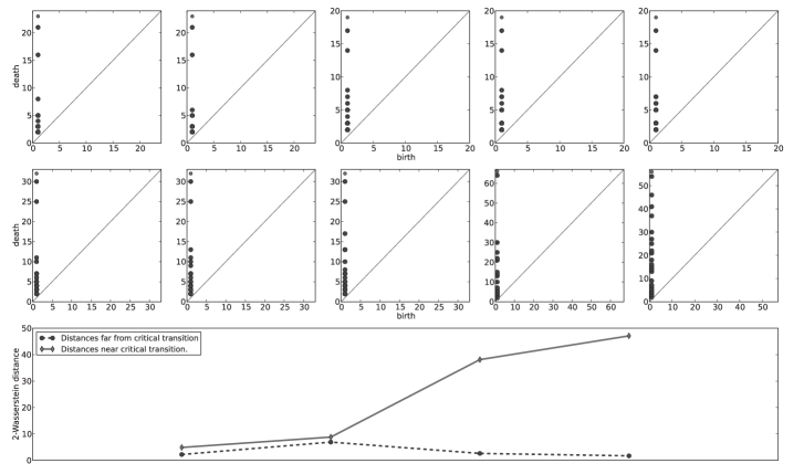
Figure 8. The $0$-persistence diagrams on the top row correspond to consecutive strings of data sampled far from the critical transition; the diagrams in the middle row correspond to consecutive strings of data sampled near the critical transition. The bottom curves describe the distances between consecutive diagrams. The plot labels are positioned between two successive diagrams with values on the $y$-axis indicating the 2-Wasserstein distances between them.

Note that the variance of the lifespans is related to the variance in the time series. An increase in the vertical spread while approaching a critical transition is consistent with the findings by the DFA method in Subsection 5.1. Also, the change observed in the clustering of the diagram coordinates is related to asymmetric or multimodal properties of the data, as mentioned in Subsection 4.2.

6. Conclusions

The substrate-depletion oscillator that we analyze in this paper is a realistic model for certain types of molecular regulation circuits studied experimentally. The methods for detecting critical transitions that we propose are suitable for the analysis of real data as well. Indeed, most of the experimental data obtained about gene regulatory networks (e.g., data obtained from microarrays, or reverse transcriptase polymerase chain reaction) is limited by background noise, and both the DFA and persistence diagram methods are robust to noise in data, as long as the noise does not overwhelm the signal. Also, in comparison with the DFA method, which necessitates a number of ‘ad-hoc’ choices of statistical parameters and procedures, the persistence diagram method appears more robust and objective.

In current and future work, we are developing a theoretical framework for the empirical criterion proposed in this paper. Namely, we plan to establish rigorously that bifurcation-induced critical transitions determine large changes in the persistence diagrams, and, conversely, large changes in the persistence diagrams imply the existence of bifurcations.

References

- [1] T. Bulter, S.-G. Lee, W.-W. Wong, E. Fung, M.R. Connor, and J.C. Liao, Design of artificial cell-cell communication using gene and metabolic networks, Proc. Natl. Acad. Sci. USA, 101 (2004), 2299–2304.
- [2] R.M. Bryce and K.B. Sprague, Revisiting detrended fluctuation analysis, Scientific Reports 2, (2012), doi:10.1038/srep00315
- [3] F. Chazal, D. Cohen-Steiner, L. J. Guibas, F. Mémoli, S. Oudot, Gromov-Hausdorff Stable Signatures for Shapes using Persistence, Computer Graphics Forum (proc. SGP 2009) (2009), 1393–1403.
- [4] F. Chazal, L.Guibas, S. Oudot, and P. Skraba, Persistence-Based Clustering in Riemannian Manifolds, Proc. 27th Annual ACM Symposium on Computational Geometry, (2011), 97–106.
- [5] F. Chazal, V. de Silva, S. Oudot, Persistence stability for geometric complexes, Geometriae Dedicata, (2013), doi: 10.1007/s10711-013-9937-z
- [6] D. Cohen-Steiner, H. Edelsbrunner, J. Harer, Y. Mileyko. Lipschitz Functions Have -Stable Persistence. Foundations of Computational Mathematics. Vol. 10 (2010), doi: 10.1007/s10208-010-9060-6
- [7] P.D. Ditlevsen and S.J. Johnsen, Tipping points: Early warning and wishful thinking, Geophysical Research Letters, Vol. 37, L19703 (2010), doi:10.1029/2010GL044486
- [8] H. Edelsbrunner and J. Harer, Persistent homology — a survey, in “Surveys on Discrete and Computational Geometry. Twenty Years Later”, 257-282, eds. J. E. Goodman, J. Pach and R. Pollack, Contemporary Mathematics 453, Amer. Math. Soc., Providence, Rhode Island, (2008).
- [9] H. Edelsbrunner and M. Morozov, Persistent Homology: Theory and Applications, Proceedings of the European Congress of Mathematics, (2012).
- [10] M. Elowitz and S.Leibler, A Synthetic Oscillatory Network of Transcriptional Regulators, Nature, Vol. 403, (2000), 335–338.
- [11] N. Fenichel, Geometric singular perturbation theory for ordinary differential equations, Journal of Differential Equations, 31 (1979), 53–98.
- [12] M. Gameiro, Y. Hiraoka, S. Izumi, M. Kramar, K. Mischaikow, and V. Nanda, A Topological Measurement of Protein Compressibility, preprint, (2013).
- [13] T.S Gardner, C.R. Cantor, and J.J. Collins, Construction of a genetic toggle switch in Escherichia coli, Nature, Vol. 403 (2000), 339–342.
- [14] J. Hasty, J. Pradines, M. Dolnik, and J.J. Collins, Noise-based switches and amplifiers for gene expression, PNAS 97 (2000), 2075–2080.
- [15] A. Hatcher,Algebraic Topology. Cambridge University Press, (2002).
- [16] R.M. Jones, Matlab code for the DFA procedure, http://criticaltransitions.wikispot.org/ (2013).
- [17] C. Kuehn, A mathematical framework for critical transitions: Bifurcations, fast-slow systems and stochastic dynamics, Physica D: Nonlinear Phenomena, 240(12) (2011), 1020 -1035.
- [18] C. Kuehn, A Mathematical Framework for Critical Transitions: Normal Forms, Variance and Applications, Journal of Nonlinear Science, DOI 10.1007/s00332-012-9158-x
- [19] M. Krupa, and P. Szmolyan, Extending geometric singular perturbation theory to nonhyperbolic points -fold and canard points in two dimensions, SIAM J. of Math. Anal. 33 (2001), 286– 314.
- [20] L. Kondic, A. Goullet, C.S. O’Hern, M. Kramar, K.Mischaikow, R.P. Behringer, Topology of force networks in compressed granular media, Europhys. Lett. 97 (2012), 54001.
- [21] M. Kramar, C++ code to compute the Wasserstein metric, Personal communication, http://www.math.rutgers.edu/ miroslav (2013).
- [22] A. Leier, P.D. Kuo, W. Banzhaf, and K. Burrage, Evolving noisy oscillatory dynamics in genetic regulatory networks, In EuroGP’06 Proceedings of the 9th European conference on Genetic Programming, LNCS 3905 (2006), 290–299.
- [23] V.N. Livina and T. M. Lenton, A modified method for detecting incipient bifurcations in a dynamical system, Geophys. Res. Lett., 34, (2007), L03712.
- [24] V. Nanda, The Perseus Software Project for Rapid Computation of Persistent Homology, http://www.math.rutgers.edu/~vidit/perseus.html
- [25] M. Nicolau, A.J. Levine, and G. Carlsson, Topology based data analysis identifies a subgroup of breast cancers with a unique mutational profile and excellent survival, PNAS,17 (2011)
- [26] B. Novak, and J.J. Tyson, Numerical analysis of a comprehensive model of M-phase control in Xenopus oocyte extracts and intact embryos, J. Cell. Sci., 106 (1993), 1153–1168.
- [27] A.A. Ptitsyn, S. Zvonic, and J.M. Gimble, Digital Signal Processing Reveals Circadian Baseline Oscillation in Majority of Mammalian Genes, PLoS Comput Biol 3 (2007), e120.
- [28] M. Scheffer et al., Early-warning signals for critical transitions, Nature, 461 (2009), 53–59.
- [29] M. Scheffer et al, Anticipating Critical Transitions, Science 338, (2012) 344, DOI: 10.1126/science.1225244
- [30] J.M.T. Thompson, and J. Sieber, Climate tipping as a noisy bifurcation: a predictive technique, IMA Journal of Applied Mathematics (2010), 1–20.
- [31] J.J. Tyson, K.C. Chen, and B. Novak, Sniffers, buzzers, toggles and blinkers: dynamics of regulatory and signaling pathways in the cell, Curr. Opin. Cell. Biol. 15(2), (2003), 221–231.
- [32] A.J. Zomorodian, Topology for Computing, Cambridge University, (2005)