Perfect clustering for stochastic blockmodel graphs via adjacency spectral embedding

Abstract

Vertex clustering in a stochastic blockmodel graph has wide applicability and has been the subject of extensive research. In this paper, we provide a short proof that the adjacency spectral embedding can be used to obtain perfect clustering for the stochastic blockmodel and the degree-corrected stochastic blockmodel. We also show an analogous result for the more general random dot product graph model.

1 Introduction

In many problems arising in the natural sciences, technology, business and politics, it is crucial to understand the specific connections among the objects under study: for example, the interactions between members of a political party; the firing of synapses in a neuronal network; or citation patterns in reference literature. Mathematically, these objects and their connections are modeled as graphs, and a common goal is to find clusters of similar vertices within a graph.

Both model-based and heuristic-based techniques have been proposed for clustering the vertices in a graphs [14, 2, 5, 19]. In this paper we focus on probabilistic performance guarantees for spectral-based techniques which have elements of both model- and heuristic-based methods [18, 20]. We study the consistency of mean squared error clustering via the adjacency spectral embedding for three nested classes of models, each an examples of latent position models [7]:

• the stochastic blockmodel where vertices in the same cluster are stochastically equivalent [8],

• the degree-corrected stochastic blockmodel where stochastic equivalence holds up to a scaling factor [9],

• and the random dot product graph where a natural vertex clustering may not exist [27].

The generality of our main result allows for the extension of our asymptotically error-free results from the rather restrictive stochastic blockmodel to more general settings.

Numerous spectral clustering procedures have been proposed and analyzed under various random graph models [4, 10, 17, 18, 20]. For example, Laplacian spectral embedding [18] and adjacency spectral embedding [20] have been shown to yield consistent clustering for the stochastic blockmodel. These results have relied on bounding the Frobenius norm difference between the embedded vertices and associated eigenvectors of the population Laplacian (in Laplacian spectral embedding) or edge probability matrix (in adjacency spectral embedding).

Relying on global Frobenius norm bounds for demonstrating consistent clustering is suboptimal, however, because in general, one cannot rule out that a diminishing but positive proportion of the embedded points contribute disproportionately to the global error. When this occurs, these “outliers” are very likely to be misclustered, and hence the best existing bounds on the Frobenius norm show that at most $O(\log(n))$ vertices will be misclustered (see [18, Theorem 3.1] and [20, Theorem 1]).

In contrast, our main technical result gives a bound (in probability) on the maximum error between individual embedded vertices and the associated eigenvectors of the edge probability matrix (see Lemma 2.5). This lemma is proved for general random dot product graphs and provides the necessary tools to improve the bounds on the error rate of mean squared error clustering in adjacency spectral embedding. The first main clustering result of this paper gives a bound on the probability that a mean square error clustering of the adjacency spectral embedding will be error-free, i.e. zero vertices will be misclustered (see Theorem 2.6).

Due to the generality of our main lemma, we are able to prove an analogous asymptotically error free clustering result in the degree-corrected stochastic blockmodel (see Theorem 4.3). Note again that the best existing results for spectral methods in the degree-corrected model assert that at most $O(\log(n))$ vertices will be misclustered [17, Theorem 4.4]. Finally, we prove a very general result that spectral clustering of random dot product graphs is strongly universally consistent in the sense of [16] (see Theorem 5.2). These extensions underly the wide utility of our approach, and we believe our main lemma to be of independent interest.

We note that the authors of [3], among others, have shown that likelihood-based techniques can be employed to achieve asymptotically error-free clustering in the stochastic blockmodel. However, likelihood based approaches are computationally intractable for very large graphs compared to our present spectral clustering approach.

2 Setting and main theorem

In the first part of this section, we will define the random dot product graph and our main tool, the adjacency spectral embedding. Next, we define the stochastic blockmodel and clustering procedure, and finally, we will state our main theorem and the supporting lemmas.

2.1 Random dot product graphs and the adjacency spectral embedding

The random dot product graph model is a convenient theoretical tool, and spectral properties of the adjacency matrix is well understood. While the stochastic blockmodel relies on an inherently non-geometric construction—indeed, each block in associated with a categorical label, and these labels determine the adjacency probabilities—the random dot product graph relies on a geometric construction in which each block is associated with a point in Euclidean space, i.e. a vector. The dot products of these vectors then determine the adjacency probabilities in the graph.

Definition 2.1 (Random Dot Product Graph (RDPG)).

A random adjacency matrix $A\sim\mathrm{RDPG}(X)$ for $X=[X_{1},\dotsc,X_{n}]^{\top}\in\mathcal{X}_{d}$ where

$$\mathcal{X}_{d}=\{Z\in\mathbb{R}^{n\times d}:ZZ^{\top}\in[0,1]^{n\times n},\mathrm{rank}(Z)=d\}$$

is said to be an instance of a random dot product graph (RDPG) if

$$\mathbb{P}[A|X]=\prod_{i>j}(X_{i}^{\top}X_{j})^{A_{ij}}{(1-X_{i}^{\top}X_{j})}^{1-A_{ij}}.$$

Remark.

In general we will denote the rows of an $n\times d$ matrix $M$ by $M_{i}^{\top}$. With this notation, in the above definition $P(A_{ij}=1)=X_{i}^{\top}X_{j}$ for all $1\leq i<j\leq n.$ We then define $P=XX^{\top}$, so that the entries of $P$ give the Bernoulli parameters for edge probabilities.

Note that, as defined above, the rank of $P$ is $d$. Let $P=[V|\widetilde{V}][S\oplus\widetilde{S}][V|\widetilde{V}]^{T}$ be the spectral decomposition of $P$ where $[V|\widetilde{V}]\in\mathbb{R}^{n\times n}$ is orthogonal, $V\in\mathbb{R}^{n\times d}$ has orthonormal columns, $S\in\mathbb{R}^{d\times d}$ is diagonal with

$$S(1,1)\geq S(2,2)\geq\dotsb\geq S(d,d)>0\text{ and }\widetilde{S}=0.$$

Importantly, we shall assume throughout this paper that the non-zero eigenvalues of $P$ are distinct, i.e., the inequalities above are strict.

It follows that there exists an orthonormal $W\in\mathbb{R}^{d\times d}$ such that $VS^{1/2}=XW$. We thus suppose that $X=VS^{1/2}$; the assumption does not lead to any loss of generality because the distribution of $A$ is invariant under orthogonal transformations of the latent positions and the clustering method considered in this paper is invariant under orthogonal transformations. This relationship between the spectral decomposition of $P$ and the latent positions $X$ for the RDPG model motivates our main tool: the adjacency spectral embedding.

Definition 2.2 (Adjacency Spectral Embedding (ASE)).

Let $\hat{V}\in\mathbb{R}^{n\times d}$ have orthonormal columns given by the eigenvectors of $A$ corresponding to the $d$ largest eigenvalues of $A$ according to the algebraic ordering. Let $\hat{S}\in\mathbb{R}^{d\times d}$ be diagonal with diagonal entries given by these eigenvalues in descending order. We define the $d$-dimensional adjacency spectral embedding of $A$ via $\hat{X}=\hat{V}\hat{S}^{1/2}$.

We shall assume, for ease of exposition, that the diagonal entries of $\hat{S}$ are positive. As will be seen later, e.g., Lemma 3.2, this assumption is justified in the context of random dot product graphs due to the concentration of the eigenvalues of $A$ around those of $P$. Recall that the rows of $\hat{X}$ will be denoted by $\hat{X}_{i}^{\top}$.

2.2 Clustering

We begin by considering the task of clustering in the $K$-block stochastic blockmodel. This model is typically parameterized by a $K\times K$ matrix of probabilities of adjacencies between vertices in each of the blocks along with the block memberships for each vertex. Here we present an alternative definition in terms of the RDPG model.

Definition 2.3 ((Positive Semidefinite) $K$-block Stochastic Blockmodel (SBM)).

We say an RDPG is an SBM with $K$ blocks if the number of distinct rows in $X$ is $K$. In this case, we define the block membership function $\tau:[n]\mapsto[K]$ to be a function such that $\tau(i)=\tau(j)$ if and only if $X_{i}=X_{j}$. For each $k\in[K]$, let $n_{k}$ be the number of vertices such that $\tau_{i}=k$, i.e. the number of vertices in block $k$.

To ease notation, we will always use $K$ to denote the number of blocks in an SBM, and we will refer to a $K$-block SBM as simply an SBM when appropriate.

Remark.

Note that a general $K$-block SBM can only be represented in this way if the $K\times K$ matrix of probabilities is positive semidefinite.

Next, we introduce mean square error clustering, which is the clustering sought by $K$-means clustering.

Definition 2.4 (Mean Square Error (MSE) Clustering).

The MSE clustering of the rows of $\hat{X}$ into $K$ blocks returns

$$\hat{C}:=\min_{C\in\mathcal{C}_{K}}\|C-\hat{X}\|_{F},\text{ where }$$

$$\mathcal{C}_{K}=\{C\in\mathbb{R}^{n\times d}:C\text{ has }K\text{ distinct rows}\},\$$

are the optimal cluster centroids for the MSE clustering. We also define the cluster membership function $\hat{\tau}:[n]\mapsto[K]$, which satisfies $\hat{\tau}_{i}=\hat{\tau}_{j}$ if and only if $\hat{C}_{i}=\hat{C}_{j}$, where $\hat{C}_{i}^{\top}$ is the $i^{\text{th}}$ row of $\hat{C}$.

In our results, we consider the MSE clustering of the rows of $\hat{X}$ in two contexts, the SBM and RDPG models defined above. We will also consider a variation of the SBM, the degree-corrected SBM, in which we perform MSE clustering on the rows of a projected version of $\hat{X}$.

2.3 Main theorems

Before stating our main results, we indicate our notation for matrix norms and we define constants to be used throughout the remaining text. For a matrix $M\in\mathbb{R}^{n\times d}$ we let $\|M\|_{2\to\infty}=\max_{i}\|M_{i}\|_{2}$, i.e. the maximum of the Euclidean norm of the rows. For a square matrix $M\in\mathbb{R}^{n\times n}$, $\|M\|_{2}=\sqrt{\text{largest eigenvalue of }M^{\top}M}$ denotes the spectral norm. The Frobenius norm of a matrix is denoted by $\|\cdot\|_{F}$.

We define:

• $\Delta=\max_{i}\sum_{j\not=i}P_{ij}$ is the maximum of the row sums of $P$;

• $d$ is the rank of $P$;

• $\gamma n=\min_{1\leq i\leq d}|S(i+1,i+1)-S(i,i)|>0$ is the minimum gap among the distinct eigenvalues of $P$;

• $K$ is the number of blocks in the SBM.

Note, $\gamma n$ is not necessarily equal to the magnitude of the smallest non-zero eigenvalue of $P$, as the gaps between consecutive non-zero eigenvalues could be smaller. We now state a technical but highly useful lemma in which we bound the maximum difference between the rows of $\hat{X}$ and the rows of an orthogonal transformation of $X$.

Lemma 2.5.

Suppose $0<\eta<1/2$ is given such that $\gamma n\geq 4\sqrt{\Delta\log{(n/\eta)}}$. Then, with probability at least $1-2\eta$, one has

$$\|\hat{X}-X\|_{2\to\infty}\leq\frac{85d\Delta^{3}\log{(n/\eta)}}{(\gamma n)^{7/2}}.$$ (1)

Remark.

The parameter $\Delta$ is the maximum expected degree for the random graph. In many models, $\gamma$ will be of the same order of the density of the graph. If the density is very small, the bound in the Eq. (1) will be large. Frequently $\Delta$ and $\gamma n$ are of the same order, so that the bound in Eq. (1) is of order $O(\log(n)/\sqrt{\gamma n})$ for $d$ fixed and $\eta$ decaying polynomially. See Example 1 for a simple illustration of how this bound can be applied. Finally, note that we always have $\Delta>\gamma n$ so that the condition in Lemma 2.5 implies that $\Delta>16\log(n/\eta)$, which allows us to use the results of [15, 25].

Lemma 2.5 gives far greater control of the errors than the previous results that were derived for the Frobenius norm $\|\hat{X}-X\|_{F}$; indeed, the latter bounds do not allow fine control of the errors in the individual rows of $\hat{X}$, and therefore can only bound the number of mis-clustered vertices via $O(\log n)$. Lemma 2.5, on the other hand, provides exactly this control and, as such, vastly improves the bounds on the error rate of MSE clustering of $\hat{X}$.

Our main theorem is the following result on the probability that mean square error clustering on the rows of $\hat{X}$ is error-free.

Theorem 2.6 (SBM).

Let $A\sim\mathrm{RDPG}(X)$ be an SBM with $K$ blocks and block membership function $\tau$ and suppose $\eta\in(0,1/2)$. Assume that

1. the non-zero eigenvalues of $P=XX^{\top}$ are distinct.

Denote the bound on $\|\hat{X}-X\|_{2\to\infty}$ in Lemma 2.5 as $\beta=\beta(d,n,\eta,\gamma)$. Let $\hat{\tau}:[n]\rightarrow[K]$ be the optimal MSE clustering of the rows of $\hat{X}$ into $K$ clusters. Let $S_{K}$ denote the symmetric group on $K$, and $\pi\in S_{K}$ a permutation of the blocks. Finally, let $n_{min}=\min_{k\in[K]}n_{k}$ be the smallest block size. If

1. for all $i,j\in[n]$ if $X_{i}\neq X_{j}$ then $\|X_{i}-X_{j}\|_{2}>6\beta\sqrt{n/n_{min}}$ and

2. the eigenvalue gap satisfies $\gamma n>4\sqrt{\Delta\log(n/\eta)},$

then with probability at least $1-2\eta$,

$$\min_{\pi\in S_{K}}|\{i\in[n]:\tau(i)\neq\pi(\hat{\tau}(i))\}|=0.$$

We remark that assumptions (A1) and (A2) are quite natural: (A1) requires that the rows of $X$ with distinct entries have some minimum separation that is large enough compared to the ratio of the number of vertices to the smallest block size and compared to the bound in Lemma 2.5. Assumption (A2) on $\gamma$ ensures a large enough gap in the eigenvalues to use Lemma 2.5. We note that Lemma 2.5 is applicable to the sparse setting, i.e., the setting wherein the average degrees of the vertices are of order $\omega(\log^{k}{n})$ for some $k\geq 2$, but that we still need sufficient separation between the distinct rows of $X$. For a simple illustration of how this theorem can be applied for a concrete model see Example 1. Finally, we admit that assumption (A0) is less natural, but it is a helpful technical restriction and it excludes a small range of parameters.

While Theorem 2.6 is proven in the SBM setting, we note that our final theorem, Theorem 5.2, is an analogous clustering result in which we prove strong universal consistency of MSE clustering for more general random dot product graphs.

Finally, we observe that Theorem 2.6 has both finite-sample and asymptotic implications. In particular, under these model assumptions, for any finite $n$, the theorem gives a lower bound on the probability of perfect clustering. We do not assert—and indeed it is easy to refute—that in the finite sample case, perfect clustering occurs with probability one. Nevertheless, we can choose $\eta=n^{-c}$ for some constant $c\geq 2$, in which case the probability of perfect clustering approaches one as $n$ tends to infinity.

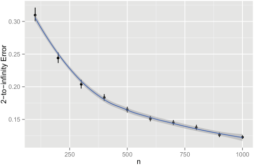
Figure 1: Mean with standard error bars of $\|\hat{X}-X\|_{2\to\infty}$ for each value of $n$ for the model in Example 1. The decay in the error is very close to $O(n^{-1/2})$.

Example 1 (Dense SBM).

Here we consider a simple concrete example where we can apply Lemma 2.5 and Theorem 2.6. Let $\nu_{1}=(.5,.4)^{\top}$ and $\nu_{2}=(0.5,-0.4)^{T}$ and let $X_{i}=\nu_{1}$ for $i=1,\dotsc,n/2$ and $X_{i}=\nu_{2}$ for $i=n/2+1,\dotsc,n$. Hence, this is a two block model and the $2\times 2$ matrix of edge probabilities is given by

$$B=\begin{pmatrix}0.41&0.09\\ 0.09&0.41\end{pmatrix}.$$

The constants in our theorem are $d=2$, $\delta=0.41n+0.09n=n/2$. The distinct eigenvalues of $P$ are $n/2,0.32n$, and 0 so the smallest gap is $0.18n$; hence $\gamma=0.18$. Lemma 2.5 can be applied as long as $0.18n\geq 4\sqrt{0.5n\log(n/\eta)}$, which will clearly hold for $n$ sufficiently large for any fixed $\eta\in(0,1/2)$. This also establishes assumptions (A0) and (A1) of Theorem 2.6.

The implication of Lemma 2.5 is that

$$\|\hat{X}-X\|_{2\to\infty}\leq\frac{85\cdot 2\cdot(0.5n)^{3}\log(n/\eta)}{(0.18n)^{7/2}}\approx\frac{8588\log(n/\eta)}{\sqrt{n}}.$$

While this bound is loose for small to moderate $n$, the asymptotic implications are clear. Empirically, Figure 1 shows the average $\|\cdot\|_{2\to\infty}$ error for this model as a function of $n$ and we see that the error becomes small much sooner and decays at a rate very close to $O(n^{-1/2})$.

For Theorem 2.6 we can compute that if $X_{i}\neq X_{j}$ then $\|X_{i}-X_{j}\|_{2}=0.8$ for all $n$ and hence since $n/n_{min}=2$ and $\beta=O(\log(n)/\sqrt{n})$, the assumption (A1) will hold for $n$ sufficiently large. Hence, for large enough $n$, there will be a very high probability that the mean square error clustering will provide perfect performance.

Example 2 (Sparse SBM).

In this example, we will illustrate some asymptotic implications of the assumptions of Theorem 2.6 in a generalization of Example 1. The SBM of the previous example is a specific instance of an SBM with edge probabilities given by

$$B=c\begin{pmatrix}a&b\\ b&a\end{pmatrix},$$ (2)

where $\tau_{i}=1$ for $i\in[n/2]$, and $\tau_{i}=2$ otherwise. In order for $P$ to be positive semidefinite we need $a>b$, and the subsequent RDPG representation is

$$\nu_{1}=\frac{\sqrt{c}}{2}\begin{pmatrix}\sqrt{a+b}+\sqrt{a-b}\\ \sqrt{a+b}-\sqrt{a-b}\end{pmatrix}\text{ and }\nu_{2}=\frac{\sqrt{c}}{2}\begin{pmatrix}\sqrt{a+b}-\sqrt{a-b}\\ \sqrt{a+b}+\sqrt{a-b}\end{pmatrix}.$$ (3)

We will investigate for what values of $a$, $b$ and $c$ the assumptions of our theorem are satisfied, noting first that (A0) is automatically satisfied. For the key constants, we can work out that the distinct eigenvalues of $P$ are $nc(a+b)/2$, $nc(a-b)/2,$ and $0$. This gives $\gamma=c\min\{b,(a-b)/2\}$. In addition, $\Delta=nc(a+b)/2$, so that assumption (A2) reads

$$nc\min\{b,(a-b)/2\}>4\sqrt{nc(a+b)\log(n/\eta)/2}.$$

We restrict ourselves to the sparse domain, and assume that $c=1/n$, $a=o(n),$ and $b=o(n).$ Assumption (A2) then becomes

$$\frac{\min\{b^{2},(a-b)^{2}/4\}}{a+b}>8\log(n/\eta).$$

Here, we have $\|\nu_{1}-\nu_{2}\|_{2}=\sqrt{2(a-b)/n}$, and assumption (A1) in this regime is equivalent to

$$\frac{\sqrt{a-b}}{(a+b)^{3}}\left(\min\{b,(a-b)/2\}\right)^{7/2}>127.5\sqrt{n}\log(n/\eta).$$

Highlighting a few special cases, we consider

• $a=O(1)$ and $b=O(1)$. In this case, our assumptions do not hold. Indeed, in [13] it is established that if $(a-b)^{2}<2(a+b)$, then clustering is impossible, and the same authors recently extended this result in [12] to show that consistent estimation is impossible for any choice of $a=O(1)$ and $b=O(1)$.

• $b=\Theta(a)=\Theta(a-b)$. In order to satisfy assumptions (A1) and (A2), it suffices that $b=\omega(\sqrt{n}\log(n)),$ and (A1) does not hold if $b=o(\sqrt{n}\log(n))$.

• $b=o(a).$ In order to satisfy assumptions (A1) and (A2), it suffices that $b/\sqrt{a}=\omega(\sqrt{\log(n)})$ and $b^{7/2}/a^{5/2}=\omega(\sqrt{n}\log(n)).$ Note that (A2) does not hold if $b/\sqrt{a}=o(\sqrt{\log(n)}),$ and (A1) does not hold if $b^{7/2}/a^{5/2}=o(\sqrt{n}\log(n)).$

• $a-b=o(b).$ In order to satisfy assumptions (A1) and (A2), it suffices that $a-b=\omega(\sqrt{\log(n)b})$ and $a-b=\omega(n^{1/8}\log(n)^{1/4}b^{3/4}).$ Note that (A2) does not hold if $a-b=o(\sqrt{\log(n)b})$, and (A1) does not hold if $a-b=o(n^{1/8}\log(n)^{1/4}b^{3/4}).$

3 Proof of Theorem 2.6

Before we prove Theorem 2.6, we first collect a sequence of useful bounds from [24, 25, 20]. We then prove two key lemmas.

Proposition 3.1.

Suppose $A\sim\mathrm{RDPG}(X)$ with $X\in\mathcal{X}_{d}$ and let $\Delta$ and $\gamma$ be as defined in Lemma 2.5. For any $\eta\in(0,1/2)$, if $\gamma n>4\sqrt{\Delta\log(n/\eta)}$, then the following occur with probability at least $1-\eta$

$$\|A-P\|_{2} \leq 2\sqrt{\Delta\log(n/\eta)},$$

$$\|\hat{V}-V\|_{F}^{2} \leq 4d\,\,\frac{\Delta\log(n/\eta)}{\gamma^{2}n^{2}}.$$

In addition, as $P$ is a non-negative matrix, $\|S\|_{2}\leq\Delta$. Thus, if $\Delta\geq 16\log{(n/\eta)}$, then provided that the above events occur, $\|\hat{S}\|_{2}\leq\min\{2\Delta,n\}$.

The next two lemmas from [1] are essential to our argument.

Lemma 3.2 ([1]).

In the setting of Proposition 3.1, if the events in Proposition 3.1 occur, then

$$\|\hat{S}-S\|_{2}\leq 18d\frac{\Delta^{2}\log{(n/\eta)}}{\gamma^{2}n^{2}}.$$

Lemma 3.3 ([1]).

In the setting of Proposition 3.1, if the events in Proposition 3.1 occur, then

$$\|V^{\top}\hat{V}-I\|_{F}\leq\frac{10d\Delta\log(n/\eta)}{\gamma^{2}n^{2}}.$$

We then have the following bound

Lemma 3.4.

In the setting of Proposition 3.1, if the events in Proposition 3.1 occur, then

$$\|AV\hat{S}^{-1/2}-\hat{X}\|_{F}\leq\frac{24\sqrt{2}d\Delta^{2}\log(n/\eta)}{(\gamma n)^{5/2}}.$$

Proof.

Let $E=A-\hat{V}\hat{S}\hat{V}^{\top}$. Denoting by $Z$ the quantity $AV\hat{S}^{-1/2}$, we have

$$\begin{split}\|Z-\hat{X}\|_{F}&=\|AV\hat{S}^{-1/2}-\hat{V}\hat{S}^{1/2}\|_{F}\\ &=\|A(V-\hat{V})\hat{S}^{-1/2}\|_{F}\\ &=\|(\hat{V}\hat{S}\hat{V}^{\top}+E)(V-\hat{V})\hat{S}^{-1/2}\|_{F}\leq C_{1}+C_{2}\end{split}$$

where $C_{1}$ and $C_{2}$ are given by

$$C_{1}=\|\hat{S}\|_{2}\|\hat{V}^{\top}(V-\hat{V})\|_{F}\|\hat{S}^{-1/2}\|_{2};\quad C_{2}=\|E\|_{2}\|V-\hat{V}\|_{F}\|\hat{S}^{-1/2}\|_{2}.$$

Note that by Proposition 3.1 and our assumption that $\gamma\sqrt{n}\geq 4\sqrt{\log(n/\eta)}$,

$$\|\hat{S}^{-1}\|_{2}\leq(\gamma n-2\sqrt{n\log n/\eta})^{-1}\leq\frac{2}{\gamma n}.$$

Combining the previous displayed equation and Lemma 3.3 yields

$$C_{1}\leq\frac{20\sqrt{2}d\Delta^{2}\log(n/\eta)}{(\gamma n)^{5/2}}.$$

Similarly, we have that $\|E\|_{2\to 2}\leq 2\sqrt{\Delta\log(n/\eta)},$ and combining this with Proposition 3.1, we bound $C_{2}$ by

$$C_{2}\leq\frac{4\sqrt{2}d\Delta\log(n/\eta)}{(\gamma n)^{3/2}},$$

from which the desired bound follows. ∎

We now use Lemma 3.2, Lemma 3.4 and Hoeffding’s inequality to prove Lemma 2.5. We note that for any matrices $A\in\mathbb{R}^{k_{1}\times k_{2}}$ and $B\in\mathbb{R}^{k_{2}\times k_{2}}$, $\|AB\|_{2\to\infty}\leq\|A\|_{2\rightarrow\infty}\|B\|_{2}$.

Proof of Lemma 2.5.

Since $X=PVS^{-1/2}$ we can add and subtract the matrix $AV\hat{S}^{-1/2}$ and $AVS^{-1/2}$ to rewrite $\hat{X}-X$ as

$$\begin{split}\hat{X}-X=A(\hat{V}-V)\hat{S}^{-1/2}+AV(\hat{S}^{-1/2}-S^{-1/2})+(A-P)VS^{-1/2}.\end{split}$$

Lemma 3.4 bounds the first term in terms of the Frobenius norm which is a bound for the $2\to\infty$ norm. For the second term, we have

$$\hat{S}^{-1/2}-S^{-1/2}=(S-\hat{S})(S^{1/2}+\hat{S}^{1/2})^{-1}(\hat{S}^{-1/2}S^{-1/2}),$$

as both $\hat{S}$ and $S$ are diagonal matrices. Applying Lemma 3.2 thus yields

$$\begin{split}\|\hat{S}^{-1/2}-S^{-1/2}\|_{2}&\leq\|S-\hat{S}\|_{2}(3/2\sqrt{\gamma n})(1/2\gamma n)\\ &\leq 24d\frac{\Delta^{2}\log{(n/\eta)}}{(\gamma n)^{7/2}},\end{split}$$

and hence

$$\begin{split}\|AV(\hat{S}^{-1/2}-S^{-1/2})\|_{2\rightarrow\infty}&\leq\|AV\|_{2\to\infty}\|\hat{S}^{-1/2}-S^{-1/2}\|_{2}\\ &\leq 48d\frac{\Delta^{3}\log{(n/\eta)}}{(\gamma n)^{7/2}}.\end{split}$$

We now bound the third term. Let $Z_{ij}$ denote the $i,j$th entry, and $Z_{i}^{\top}$ the $i$th row, of the $n\times d$ matrix $(A-P)V$. Observe that

$$\|(A-P)V\|_{2\rightarrow\infty}=\max_{i}\|Z_{i}\|_{2}\leq\sqrt{d}\max_{i,j}|Z_{i,j}|.$$

Next, since

$$Z_{ij}=\sum_{k=1}^{n}(A_{ik}-P_{ik})(V)_{kj},$$

we see that $Z_{ij}$ is a sum of $n$ independent, mean zero random variables $R_{k}(ij)=(A_{ik}-P_{ik})(V)_{kj}$, and $|R_{k}(ij)|\leq|(V)_{kj}|$. Since $V$ has orthonormal columns, $\sum_{k}(V)^{2}_{kj}=1$. Therefore, Hoeffding’s inequality implies

$$\mathbb{P}\Bigl{(}|Z_{ij}|>\sqrt{\tfrac{1}{2}\log(2nd/\eta)}\,\,\Bigr{)}\leq\frac{\eta}{nd}.$$

Since there are $nd$ entries $Z_{ij}$, a simple union bound ensures that

$$\mathbb{P}\Bigl{(}\max_{i,j}|Z_{ij}|>\sqrt{\tfrac{1}{2}\log(2nd/\eta)}\,\,\Bigr{)}\leq\eta,$$

and consequently that

$$\mathbb{P}\Bigl{(}\|(A-P)V\|_{2\rightarrow\infty}>\sqrt{\tfrac{d}{2}\log(2nd/\eta)}\,\,\Bigr{)}\leq\eta.$$

The third term can therefore be bounded as

$$\begin{split}\|(A-P)VS^{-1/2}\|_{2\to\infty}\leq\|(A-P)V\|_{2\to\infty}\|S^{-1/2}\|_{2}\leq\sqrt{\frac{d\log{(2nd/\eta)}}{2\gamma n}}\end{split}$$

with probability at least $1-\eta$. Combining the bounds for the above three terms yields Lemma 2.5. ∎

Proof of Theorem 2.6.

Let $r:=\beta\sqrt{n/n_{min}}.$ We assume that the event in Lemma 2.5 occurs and show that this implies the result. Since $X$ has $K$ distinct rows, it follows that

$$\|\hat{C}-\hat{X}\|_{F}\leq\|X-\hat{X}\|_{F}\leq\beta\sqrt{n}.$$

Let $\mathcal{B}_{1},\mathcal{B}_{2},\ldots,\mathcal{B}_{K}$ be $L^{2}$-balls with radii $2r$ around the $K$ distinct rows of $X$. By the assumptions in Theorem 2.6, these balls are disjoint. Suppose there exists $k\in[K]$ such that $\mathcal{B}_{k}$ does not contain any rows of $\hat{C}$. Then $\|\hat{C}-X\|_{F}>2r\sqrt{n_{min}}$, as for each $k$, no row of $\hat{C}$ is within $2r$ of the (at least $n_{min}$) rows of $X$ in $\mathcal{B}_{k}$. This implies that

$$\begin{split}\|\hat{C}-\hat{X}\|_{F}&\geq\|\hat{C}-X\|_{F}-\|\hat{X}-X\|_{F}\\ &>2r\sqrt{n_{min}}-\beta\sqrt{n}\\ &>2\beta\sqrt{\frac{n}{n_{min}}}\sqrt{n_{min}}-\beta\sqrt{n}=\beta\sqrt{n},\end{split}$$

a contradiction. Therefore, $\|\hat{C}-X\|_{2\to\infty}\leq 2r$. Hence, by the pigeonhole principle, each ball $\mathcal{B}_{k}$ contains precisely one distinct row of $\hat{C}$.

If $X_{i}=X_{j}$, then both $\hat{C}_{i}$ and $\hat{C}_{j}$ are elements of $\mathcal{B}_{\tau(i)}$, and since there is exactly one distinct row of $\hat{C}$ in $\mathcal{B}_{k}$, $\hat{C}_{i}=\hat{C}_{j}$. Conversely, if $\hat{C}_{i}\not=\hat{C}_{j}$, then $X_{i}$ and $X_{j}$ are in disjoint balls $\mathcal{B}_{k}$ and $\mathcal{B}_{k^{\prime}}$ for some $k,k^{\prime}\in[K]$, implying that $X_{i}\not=X_{j}$. Thus, $X_{i}=X_{j}$ if and only if $\hat{C}_{i}=\hat{C}_{j}$, proving the theorem. ∎

4 Degree corrected SBM

In this section we extend our results to the degree corrected SBM [9].

Definition 4.1 (Degree Corrected Stochastic Blockmodel (DCSBM)).

We say an RDPG is a DCSBM with $K$ blocks if there exist $K$ unit vectors $y_{1},\dotsc,y_{K}\in\mathbb{R}^{d}$ such that for each $i\in[n]$, there exists $k\in[K]$ and $c_{i}\in(0,1)$ such that $X_{i}=c_{i}y_{k}$.

Remark.

This model is inherently more flexible than the standard SBM because it allows for vertices within each block/community to have different expected degrees. This flexibility has made it a popular choice for modeling network data [9].

For this model, we introduce $Y\in\mathbb{R}^{n\times d}$ via $Y_{i}^{\top}=y_{\tau(i)}^{\top}$, so that each row of $Y$ has unit $L^{2}$-norm. As demonstrated in [17], a key to spectrally clustering DCSBM graphs is to project the spectral embedding onto the unit sphere, yielding an estimate of $Y$ rather than an estimate of $X$. As such, let $\hat{Y}=\mathrm{diag}(\hat{X}\hat{X}^{\top})^{-1/2}\hat{X}$ where $\mathrm{diag}(\cdot)$ denotes the operation of setting all the off-diagonal elements of the argument to 0. If we denote the unit sphere in $\mathbb{R}^{d}$ by $\mathcal{S}=\{x\in\mathbb{R}^{d}:\|x\|_{2}=1\}$, then $\hat{Y}$ is the projection of $\hat{X}$ on $\mathcal{S}$. See Figure 2 for a simple example of this projection step.

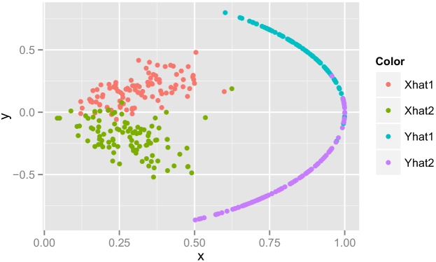
Figure 2: Example of $\hat{X}$ (the red and green points) and $\hat{Y}$ (the blue and purple points) for a 2-block DCSBM with latent positions $y_{1}=[1/5,2\sqrt{6}/5]$ and $y_{2}=[2\sqrt{6}/5,1/5]$ and 100 vertices in each block. The $c_{i}$’s are i.i.d. Uniform(0.2,0.5).

Our next lemma is the analogue of Lemma 2.5 in the DCSBM setting, allowing us to tightly control the errors in the individual rows of $\hat{Y}$.

Lemma 4.2.

In the setting of Lemma 2.5, let the $n\times d$ matrices $\widetilde{Y},\hat{Y}\in\mathcal{S}$ be the projections of $X$ and $\hat{X}$, respectively, onto $\mathcal{S}$. Let $c_{min}=\min_{i\in[n]}\|X_{i}\|_{2}$. If $\|\hat{X}-X\|_{2\to\infty}\leq\beta$, then

$$\|\hat{Y}-\widetilde{Y}\|_{2\to\infty}\leq\frac{2\beta}{c_{min}}.$$

Proof.

We have $\widetilde{Y}_{i}=(\|X_{i}\|_{2})^{-1}X_{i}$ and $\hat{Y}_{i}=(\|\hat{X}_{i}\|_{2})^{-1}\hat{X}_{i}$. Straightforward calculations then yield

$$\begin{split}\|\widetilde{Y}_{i}-\hat{Y}_{i}\|_{2}&=\Bigl{\|}\frac{X_{i}}{\|X_{i}\|_{2}}-\frac{\hat{X}_{i}}{\|\hat{X}_{i}\|_{2}}\Bigr{\|}_{2}\\ &=\Bigl{\|}\frac{X_{i}}{\|X_{i}\|_{2}}-\frac{\hat{X}_{i}}{\|X_{i}\|_{2}}+\frac{\hat{X}_{i}}{\|X_{i}\|_{2}}-\frac{\hat{X}_{i}}{\|\hat{X}_{i}\|_{2}}\Bigr{\|}_{2}\\ &\leq\frac{\|X_{i}-\hat{X}_{i}\|_{2}}{\|X_{i}\|_{2}}+\|\hat{X}_{i}\|_{2}\Bigl{(}\frac{1}{\|X_{i}\|_{2}}-\frac{1}{\|\hat{X}_{i}\|_{2}}\Bigr{)}\leq 2\frac{\|X_{i}-\hat{X}_{i}\|_{2}}{\|X_{i}\|_{2}}\leq\frac{2\beta}{c_{\mathrm{min}}}\end{split}$$

as desired. ∎

As in Theorem 2.6, this allows us to bound the probability of error-free MSE clustering.

Theorem 4.3 (Degree-corrected SBM).

Suppose $A\sim\mathrm{RDPG}(X)$ and is a DCSBM with $K$ blocks and block membership function $\tau$ and suppose $\eta\in(0,1/2)$. Let $y_{1},\dotsc,y_{K}$ be the $K$ unit vectors for the DCSBM and let $c_{min}$ denote the smallest scaling factor. Let $\gamma,\beta$ be as in Theorem 2.6. Suppose $r>0$ is such that for all $i,j\in[K]$, $\|y_{i}-y_{j}\|_{2}>6r$. Let $\hat{\tau}:[n]\rightarrow[K]$ be the optimal MSE clustering of the rows of $\hat{Y}$, the projection of $\hat{X}$ onto $\mathcal{S}$, into $K$ clusters. Finally, let $n_{min}=\min_{k\in[K]}n_{k}$ be the smallest block size. If

$$r>(2\beta\sqrt{n/n_{min}})/c_{min}\text{ and }\gamma n>4\sqrt{\Delta\log(n/\eta)},$$

then with probability at least $1-2\eta$,

$$\min_{\pi\in S_{K}}|\{i\in[n]:\tau(i)\neq\pi(\hat{\tau}(i))\}|=0.$$

The proof of this theorem follows mutatis mutandis from the proof of Theorem 2.6.

5 Strong universal consistency

We next show how our methodology can be used to prove strong universal consistency of $K$-means clustering (as considered in [16]) in the general RDPG setting. Specifically, suppose that $\{X_{1},\dots,X_{n}\}$ is a sample of independent observations from some common compactly supported distribution $F$ on $\mathbb{R}^{d}$. Denote by $F_{n}$ the empirical distribution of the $\{X_{i}\}$, and let $C$ be a set containing $K$ or fewer points. Suppose that $\phi\colon[0,\infty)\mapsto[0,\infty)$ is a continuous, nondecreasing function with $\phi(0)=0$. Now define $\Phi(C,F_{n})$ and $\Phi(C,F)$ by

$$\Phi(C,F_{n})=\int\bigl{(}\min_{c\in C}\phi(\|x-c\|)\bigr{)}dF_{n}(x),$$

$$\Phi(C,F)=\int\bigl{(}\min_{c\in C}\phi(\|x-c\|)\bigr{)}dF(x).$$

The problem of $K$-means mean square error clustering given $\{X_{1},\dots,X_{n}\}$ can then be viewed as the minimization of $\Phi(A,F_{n})$ for $\phi(r)=r^{2}$ over all sets $C$ containing $K$ or fewer elements. The strong consistency of $K$-means clustering corresponds then to the following statement.

Theorem 5.1 ([16]).

Suppose that for each $k=1,\dots,K$, there is a unique set $\bar{C}_{k}$ for which

$$\Phi(\bar{C}_{k},F)=\inf_{C\colon|C|=k}\Phi(C,F).$$

For any given $\{X_{1},\dots,X_{n}\}$, denote by $C_{n}$ a minimizer of $\Phi(C,F_{n})$ over all sets $C$ containing $K$ or fewer elements. Then $C_{n}\rightarrow\bar{C}_{K}$ almost surely and $\Phi(C_{n},F_{n})\rightarrow\Phi(\bar{C}_{K},F)$ almost surely.

We now state the counterpart to Theorem 5.1 for the RDPG setting.

Theorem 5.2 (RDPG).

Let $A\sim\mathrm{RDPG}(X)$, where the latent positions are sampled from some common compactly supported distribution $F$. Let $\hat{F}_{n}$ be the empirical distribution of the $\{\hat{X}_{i}\}_{i=1}^{n}$. Denote by $\hat{C}_{n}$ a minimizer of $\Phi(C,\hat{F}_{n})$ over all sets $C$ containing $K$ or fewer elements. Then provided that the conditions in Theorem 5.1 holds for $F$, $\hat{C}_{n}\rightarrow\bar{C}_{K}$ almost surely, and furthermore, $\Phi(\hat{C}_{n},\hat{F}_{n})\rightarrow\Phi(\bar{C}_{K},F)$ almost surely.

Proof.

We can suppose, without loss of generality, that $F$ is a distribution on a totally bounded set, say $\Omega$. Let $\mathcal{G}$ denote the family of functions of the form $g_{C}(x)=\min_{c\in C}\phi(\|x-c\|_{2})$ where $C$ ranges over all subsets of $\Omega$ containing $K$ or fewer points. The theorem is equivalent to showing

$$\sup_{g\in\mathcal{G}}\Bigl{|}\int g\,\,d\hat{F}_{n}-\int g\,\,dF\Bigr{|}\overset{\mathrm{a.s.}}{\longrightarrow}0.$$

By Theorem 5.1, we know that

$$\sup_{g\in\mathcal{G}}\Bigl{|}\int g\,\,dF_{n}-\int g\,\,dF\Bigr{|}\overset{\mathrm{a.s.}}{\longrightarrow}0.$$

and so the theorem holds provided that

$$\sup_{g\in\mathcal{G}}\Bigl{|}\int g\,\,d\hat{F}_{n}-\int g\,\,dF_{n}\Bigr{|}=\sup_{g\in\mathcal{G}}\Bigl{|}\frac{1}{n}\sum_{i=1}^{n}\bigl{\{}\min_{c\in C}\phi(\|\hat{X}_{i}-c\|_{2})-\min_{c\in C}\phi(\|X_{i}-c\|_{2})\bigr{\}}\Bigr{|}\overset{\mathrm{a.s.}}{\longrightarrow}0.$$

Let $s_{i}$ denote the summand in the above display. We then have the following bound

$$|s_{i}|\leq\max_{c\in C}\{\bigl{|}\phi(\|\hat{X}_{i}-c\|_{2})-\phi(\|X_{i}-c\|_{2})\bigr{|}\};$$

and hence

$$\begin{split}\Bigl{|}\frac{1}{n}\sum_{i=1}^{n}s_{i}\Bigr{|}&\leq\frac{1}{n}\sum_{i=1}^{n}\sum_{c\in C}|\phi(\|\hat{X}_{i}-c\|_{2})-\phi(\|X_{i}-c\|_{2})|\\ &\leq K\max_{i}\max_{c\in C}|\phi(\|\hat{X}_{i}-c\|_{2})-\phi(\|X_{i}-c\|_{2})|.\end{split}$$

We thus have the bound

$$\sup_{g\in\mathcal{G}}\Bigl{|}\frac{1}{n}\sum_{i=1}^{n}s_{i}\Bigr{|}\leq K\sup_{c\in\Omega}\max_{i}|\phi(\|\hat{X}_{i}-c\|_{2})-\phi(\|X_{i}-c\|_{2})|.$$

Now, by Lemma 2.5, $\sup_{i}\|\hat{X}_{i}-X_{i}\|_{2}$ converges to $0$ almost surely. Since $\phi$ is continuous on a compact set, it is uniformly continuous. Thus

$$\sup_{c\in\Omega}\sup_{i}|\phi(\|\hat{X}_{i}-c\|_{2})-\phi(\|X_{i}-c\|_{2})|\overset{\mathrm{a.s.}}{\longrightarrow}0$$

as desired. ∎

6 Discussion

Lemma 2.5 provides a bound on the $2$-to-$\infty$ norm of the difference between $\hat{X}$ and $X$. The ability to control the errors of individual rows of $\hat{X}$ allows us to prove asymptotically almost surely perfect clustering in the SBM and DCSBM, a substantive improvement on the best existing spectral clustering results.

Our approach can be easily modified to prove several extensions of Theorem 2.6. For example, we can consider the special case in which the constants are fixed in $n$ and $n_{min}=\Theta(n)$, whereupon the conditions of Theorem 2.6 are all satisfied for $n$ sufficiently large. In this setting, we can further suppose that there are $K$ positions $\xi_{1},\dotsc,\xi_{k}$ and $\mathbb{P}[X_{i}=\xi_{k}]=\pi_{k}$ for some $\pi_{k}>0$, i.e. a mixture of point masses. In other words, this is an stochastic block model with independent, identically distributed block memberships (that are not fixed) across vertices. Proving that the number of errors converges almost surely to zero is then an easy application of Theorem 2.6. Furthermore, our methods can be extended to alternate clustering procedures, such as Gaussian mixture modeling (see [22]) or hierarchical clustering.

Indeed, one can construct many examples where perfect performance isachieved asymptotically (see Examples 1 and 2). We will not detail all regimes explicitly, but rather note that this theory can be easily applied to handle a growing number of blocks, possibly impacting $d$, $\gamma$ and $n_{min}$, and moderately sparse regimes, impacting $\gamma$.

We believe Lemma 2.5 to be of independent interest apart from clustering. Indeed, Lemma 2.5 is a key result in proving consistency of a divide-and-conquer seeded graph matching procedure [11]. The lemma also leads to an easy proof of the strong consistency of $k$-nearest-neighbors for vertex classification, thereby extending the results of [21]. The lemma is a key component of the construction of a consistent two-sample graph hypothesis test [23]. Additionally, we are exploring the implications of the lemma on parameter estimation for more general latent position random graphs.

The DCSBM is inherently more general than the SBM, and has key properties useful in modeling group structures in graphs. In [17], the authors provide complementary results for spectral analysis of the DCSBM without requiring lower bounds on the degrees; however, in turn, they obtain less-than-perfect clustering. Our results are the first to show that, depending on model parameters, the probability of perfect clustering tends to one as the number of vertices tends to infinity. The keys to the easy extension of these results to more general models are Lemmas 2.5 and 3.4, stated here in the RDPG setting.

For a general RDPG, there may not be a “natural” community structure. Nonetheless, the strong universal consistency result of Theorem 5.2 ensures that clustering the embedded graph will be asymptotically equivalent to the clustering the true latent positions. Finding the $k$-centers of the estimated latent positions provides one way to approximate the distribution of the latent positions as a mixture of point masses corresponding to an SBM, where the $k$ distinct latent positions are given by the $k$-centers. Approximating a more general graph distribution as a stochastic blockmodel has been studied by [26] and [6], and here we have detailed one spectral solution to this problem. If $k$ is chosen appropriately, these approximations yield suitably parsimonious distributions that can be used for understanding large complex graphs, without requiring the estimation of a correspondingly complex distribution.

References

- [1] A. Athreya, V. Lyzinski, D. J. Marchette, C. E. Priebe, D. L. Sussman, and M. Tang. A limit theorem for scaled eigenvectors of random dot product graphs. Arxiv preprint. http://arxiv.org/abs/1305.7388, 2013.
- [2] P. J. Bickel and A. Chen. A nonparametric view of network models and Newman-Girvan and other modularities. Proc. Natl. Acad. Sci. USA, 106:21068–73, 2009.
- [3] P. J. Bickel, A. Chen, and E. Levina. The method of moments and degree distributions for network models. Ann. Statist., 39:38–59, 2011.
- [4] K. Chaudhuri, F. Chung, and A. Tsiatas. Spectral partitioning of graphs with general degrees and the extended planted partition model. In Proceedings of the 25th conference on learning theory, 2012.
- [5] D. S. Choi, P. J. Wolfe, and E. M. Airoldi. Stochastic blockmodels with a growing number of classes. Biometrika, 99:273–284, 2012.
- [6] David Choi, Patrick J Wolfe, et al. Co-clustering separately exchangeable network data. The Annals of Statistics, 42(1):29–63, 2014.
- [7] P. D. Hoff, A. E. Raftery, and M. S. Handcock. Latent space approaches to social network analysis. Journal of the American Statistical Association, 97(460):1090–1098, 2002.
- [8] P. W. Holland, K. Laskey, and S. Leinhardt. Stochastic blockmodels: First steps. Social Networks, 5:109–137, 1983.
- [9] B. Karrer and M. E. J. Newman. Stochastic blockmodels and community structure in networks. Phys. Rev. E, 83, 2011.
- [10] J. Lei and A. Rinaldo. Consistency of spectral clustering in sparse stochastic blockmodels. Arxiv preprint. http://arxiv.org/abs/1312.2050, 2013.
- [11] V. Lyzinski, D. L. Sussman, D. E. Fishkind, H. Pao, L. Chen, J. T. Vogelstein, and C. E. Priebe. Spectral clustering for divide-and-conquer graph matching. Arxiv preprint. http://arxiv.org/abs/1310.1297, 2014.
- [12] E. Mossel, J. Neeman, and A. Sly. Consistency thresholds for binary symmetric block models. arXiv preprint arXiv:1407.1591, 2014.
- [13] E. Mossel, J. Neeman, and A. Sly. Stochastic block models and reconstruction. Probability Theory and Related Fields, In press.
- [14] M. E. J. Newman. Modularity and community structure in networks. Proceedings of the National Academy of Sciences, 103(23):8577–8582, 2006.
- [15] R. I. Oliveira. Concentration of the adjacency matrix and of the laplacian in random graphs with independent edges. Arxiv preprint http://arxiv.org/abs/0911.0600, 2010.
- [16] D. Pollard. Strong consistency of -means clustering. Ann. Statist., 9:135–140, 1981.
- [17] Tai Qin and Karl Rohe. Regularized spectral clustering under the degree-corrected stochastic blockmodel. arXiv preprint., 2013.
- [18] K. Rohe, S. Chatterjee, and B. Yu. Spectral clustering and the high-dimensional stochastic blockmodel. Ann. Statist., 39:1878–1915, 2011.
- [19] T. A. B. Snijders and K. Nowicki. Estimation and Prediction for Stochastic Blockmodels for Graphs with Latent Block Structure. J. Classification, 14:75–100, 1997.
- [20] D. L. Sussman, M. Tang, D. E. Fishkind, and C. E. Priebe. A consistent adjacency spectral embedding for stochastic blockmodel graphs. Journal of the American Statistical Association, 107(499):1119–1128, 2012.
- [21] D. L. Sussman, M. Tang, and C. E. Priebe. Consistent latent position estimation and vertex classification for random dot product graphs. IEEE T. Pattern. Anal., 36:48–57, 2014.
- [22] S. Suwan, D.S Lee, R. Tang, D.L. Sussman, M. Tang, and C.E. Priebe. Empirical bayes estimation for the stochastic blockmodel. Arxiv preprint at arxiv.org/abs/1405.6070, 2014.
- [23] M. Tang, A. Athreya, D. L. Sussman, V. Lyzinski, and C. E. Priebe. A semiparametric two-sample hypothesis testing problem for random dot product graphs. arXiv preprint. http://arxiv.org/abs/1403.7249, 2014.
- [24] M. Tang, D. L. Sussman, and C. E. Priebe. Universally consistent vertex classification for latent position graphs. Ann. Statist., 41:1406 – 1430, 2013.
- [25] J. A. Tropp. Freedman’s inequality for matrix martingales. Electron. Commun. Probab, 16:262–270, 2011.
- [26] P. J. Wolfe and S. C. Olhede. Nonparametric graphon estimation. arXiv preprint at http://arxiv.org/abs/1309/5936, 2013.
- [27] S. Young and E. Scheinerman. Random dot product graph models for social networks. In Proceedings of the 5th international conference on algorithms and models for the web-graph, pages 138–149, 2007.