Colors of c-type RR Lyrae Stars and Interstellar Reddening

Abstract

RR Lyrae stars pulsating in the fundamental mode have long been used to measure interstellar reddening, based on their observed uniformity of $B-V$ color at minimum light after small corrections for metallicity and period are applied. However, little attention has been paid to the first overtone pulsators (RRc or RR1). We present new $V-I$ observations of field RRc stars, supplemented with published data from uncrowded RRc in globular clusters. Preliminary results indicate the RRc colors are correlated with period, but appear to be independent of the stars’ metallicity. The scatter around the period-color relation is slightly larger than a comparable relation for RRab. Thus, RRc can be useful indicators of line of sight reddening toward old stellar systems, particularly when multiple stars are available as in Oosterhoff II globular clusters and metal-poor galaxies.

I Introduction

The first figure of Horace Smith’s book on RR Lyrae stars (RRL) demonstrates the difference between fundamental mode pulsators (RRab or RR0) and the first overtone stars (RRc or RR1): the latter have shorter periods, typically $0.20<P<0.45$ days, and smaller amplitudes, typically $\Delta V\approx 0.5$ mag (Smith 1995). Preston (1964) first noted that RRab have a constant color over the ”minimum light” phase interval of $0.5<\phi<0.8$, and Sturch (1966) utilized this to develop a tight relation between intrinsic $B-V$ color, pulsation period, and the photometric metallicity indicator $\delta(U-B)$. Blanco (1992) improved this relation by adding more stars and casting the metallicity in terms of the spectroscopic $\Delta S$ index of the strength of the Ca II K line. Walker (1990) provided a similar relation using [Fe/H] to indicate metallicity.

Since then, more and more RRL photometry has been done using red-sensitive CCDs in the $VI$ bands. Mateo et al. (1995) showed that $V-I$ colors can also be used to determine interstellar reddening, and that the metallicity sensitivity is weaker than for $B-V$ based on their sample of a dozen stars drawn from the literature. Day et al. (2002) and Guldenschuh et al. (2005) refined and extended this relation for RRab using new observations of six southern stars. Kunder et al. (2010) extended the relation to $V-R$ colors.

Despite this extensive development for RRab stars, little work has been done to calibrate a reddening relation for RRc. One example is the relation presented in McNamara (2011),

$$(\langle B\rangle-\langle V\rangle)_{0}=0.048+0.501P,$$ (1)

where the angled brackets indicate the intensity mean magnitude over all phases. McNamara derived this relation for the RRc in M3, and extended it to other metallicities using a color correction based on model atmospheres. Our goal in this study is to provide reliable calibrations for $B-V$ and $V-I$ colors based on a larger sample of RRc stars spanning a wide range in metallicity and including stars in both globular clusters and the Galactic field.

II Data

Over the last decade, we have acquired numerous $VI$ images of RRL using the 0.5-m Cassegrain telescope and Apogee Ap6e CCD camera located on the BGSU campus. Here, we present data for 11 RRc. For each star, all-sky photometry was obtained using the WIYN 0.9-m telescope at Kitt Peak in order to calibrate the $VI$ magnitudes of about ten surrounding comparison stars to the Landolt (1992) scale, and thereby enable the transformation of the differential photometry of the RRc taken at BGSU onto the standard $VI$ system.

Several southern RRc were observed using the PROMPT 0.4-m telescopes on Cerro Tololo, Chile. Differential photometry was derived from most images, and calibrated to the standard $VI$ system using Landolt (1992) standards taken on one photometric night.

Additional $BVI$ data were gleaned from published studies of RRc in globular clusters. For consistency with the field star data, we preferentially selected studies with photometry tied to Landolt (1992) or Stetson (2000) standard stars. Table 1 shows the clusters we have currently utilized, including the metallicity and reddening from the Harris (1996) compilation, the Oosterhoff type, the number of RRc stars in the cited reference, the filters employed, the standard stars used to calibrate the photometry, the method of photometry, and the reference to the study from which the photometry was taken. In most cases, we were able to retrieve the original time series photometry, so we can plot the light curves in all available passbands and perform our own statistical analysis on the data. For many of these clusters, more recent photometry is available, but it tends to be of variables in the inner, crowded region of the cluster. This summer, we are in the process of adding 3-4 new clusters to the analysis.

lccccccll Globular Clusters 0pt

NGC & [Fe/H] $E(B-V)$ Oo $N_{RRc}$ Filters Stdsa Methodb Reference

1851 & –1.18 0.02 I 7 $BVI$ L92 DAO Walker (1998)

5904=M5 –1.29 0.03 I 14 $VI$ L92 DAO Reid (1996)

5272=M3 –1.50 0.01 I 47 $BVI$ S00 ISIS Benkő et al. (2006)

4171 –1.80 0.02 I? 10 $BVI$ S00 DAO Stetson et al. (2005)

4590=M68 –2.23 0.05 II 16 $BVI$ L92 DAO Walker (1994)

Standard stars from Landolt (1992) or Stetson (2000). Photometry derived from DAOPHOT (Stetson 1987) or ISIS (Alard, 2000).

Light curves for two typical stars are shown in the top panels of Figure 1. For stars with non-contemporaneous $BVI$ observations we created color curves by creating a series of twenty phase bins, each 0.05 phase units wide, and calculating the magnitude-mean $B$, $V$, and $I$ in each bin, and then calculating $B-V$ and $V-I$ in each bin. Results are shown in the bottom panels of Figure 1.

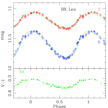
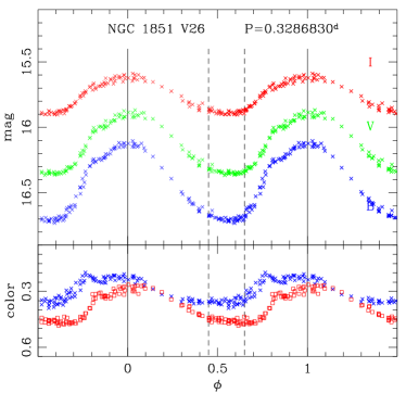
Figure 1: The light and color curves for the field star BX Leo observed at BGSU $(left)$, and the globular cluster star V26 in NGC 1851 from Walker (1998), which has $C_{C}=1~{}(right)$. The red and blue color curves for V26 show $V-I$ and $B-V$, respectively.

Because photometric crowding and blending can bias photometry in globular clusters, we visually inspected the environs of each variable star on a wide-field, mosaicked CCD image provided with the Stetson (2000) standards, using finder charts or equatorial coordinates to identify the variable. We assigned the star a “crowding class” ($C_{C}$) on a 0-4 scale, where 0 indicates an isolated star comparable to most field stars, and 4 indicates a badly blended image. While admittedly more subjective than the separation index of Stetson, Bruntt & Grundahl (2003), we do not have access to the original CCD images or DAOPOT photometry from which to calculate the separation index. The crowding class has the advantage that it includes stars not in the DAOPHOT star list, such as badly saturated stars, and it considers the level of unresolved background light. It is also a good training exercise for acquainting new students with astronomical image analysis and star field recognition.

The RRL-rich cluster M3 provides an opportunity to check how photometry may be biased by stellar crowding, though this cluster is far from the most crowded in our list. In Figure 2 we show the intensity-mean magnitudes and colors of the RRc in M3 plotted against their crowding class. The right-side panels show generalized histograms (replacing each binned point in a normal histogram with a unit Gaussian having $\sigma=0.02$ mag) of the stars having $0\leq C_{C}\leq 2$ (solid curves) and for all stars (dotted curves). In the top panel, we would expect to see more crowded stars show a tendency to be brighter and span a wider range of magnitudes as neighbor stars blend and merge with the target variable. We see some of this behavior, but there is also vertical scatter at every crowding class, perhaps due to binary companions. The colors show more affect of crowding: in both cases the scatter increases with crowding class, though some of the scatter seen in $\langle V\rangle-\langle I\rangle$ at all crowding classes is attributable to the strong period-dependence described below. Also shown in the figure is the fact that the point-to-point scatter in a star’s light curve tends to increase with crowding class, suggesting that the effects of crowding vary from image to image depending on factors like seeing, sky background, etc. From this analysis, we conclude that the photometry of stars with $0\leq C_{C}\leq 2$ is generally trustworthy, while that of stars with $C_{C}=3$ or 4 becomes increasingly less so. Since our goal is to get the best possible mean colors, rather than a complete sample, and many clusters have abundant RRc, we can reject stars with $C_{C}\geq 3$.

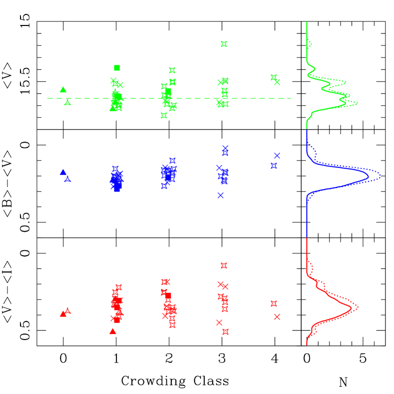
Figure 2: The left panels show the intensity-mean $V$ magnitude (top), $B-V$ color (middle), and $V-I$ color (bottom) as functions of crowding class for the RRc stars in M3. The symbols indicate light curves with little scatter (solid), some scatter (open), and large scatter (crosses), with 3-point and 4-point symbols indicating data from the Schmidt and RCC telescopes, respectively (Benkő et al. 2006). The right panels show generalized histograms of these distributions.

III Analysis

The color of an RRL can be calculated in many ways. Past studies of RRab stars have focused on the mean magnitude-averaged color during minimum light, defined as the interval between phases of 0.5 and 0.8 (Sturch 1966), where the color is approximately constant. The advantage of this definition is that when the number of data points is small, as in a program to find RRL in a distant galaxy (e.g., M33, Sarajedini et al. 2006) or heavily reddened cluster (e.g., NGC 6441, Pritzl et al. 2003), a single observation in this phase interval may result in a better reddening estimate than the average of all the data points over a light curve with sparse or gappy phase coverage. A disadvantage of minimum light colors, noted by McNamara (2011), is that many extant studies (including those listed in Table 1) do not tabulate minimum-light colors, necessitating recovery of the original time-series data and its analysis.

The aim of our present study is to maximize the utility of our $V-I$ and $B-V$ color data by expressing the color in terms of all three of the current definitions, and to explore which definition might produce the smallest scatter and hence serve as the best reddening indicator. We calculate minimum light colors from the original time-series, but adopt from each study their tabulated intensity-mean colors, $\langle V\rangle-\langle I\rangle$ (where the $\langle\rangle$ notation indicates an intensity-mean magnitude taken over all phases), and the magnitude-mean colors, ${V-I}_{mag}$ taken over all phases (our calculated values usually match the tabulated ones to several 0.001 mag).

Our first task is to determine whether RRc stars have a minimum light phase interval in which the color is roughly constant. We selected about four stars from each cluster that have low crowding class, light curves with little scatter, and which span a wide range in period. Figure 3 shows the color curves of these stars after correction for the small reddenings listed in Table 1. The goal was to get a representative sample of light curve shapes and periods at each cluster’s metallicity. It is clear from Figure 3 that the phase interval used for RRab, $0.5\leq\phi\leq 0.8$, is too large for the more sinusoidal light curve shapes of RRc. However, star-to-star variations in color due to period (see below) tend to confuse and mask the behavior of the RRc near minimum light. Following the method used by Sturch (1966), we vertically shift each light curve so they match at a common phase point, in our case we chose $\phi=0.525$ as shown in Figure 4. For $B-V$, it seems that many stars have a fairly constant color over the phase interval $0.45\leq\phi\leq 0.65$, but in $V-I$ the stars have a wider range of color curve shapes so that some stars become bluer during this phase interval while others become redder. As the summer progresses and we add more clusters to Figures 3 and 4, we will perform a quantitative analysis like Sturch (1966) to define the best minimum light interval for RRc stars, but for now it appears that $0.45\leq\phi\leq 0.65$ provides a good working definition.

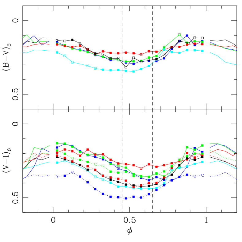
Figure 3: Color curves for a selection of RRc in globular clusters. The phase points 0.45 and 0.65 are marked.

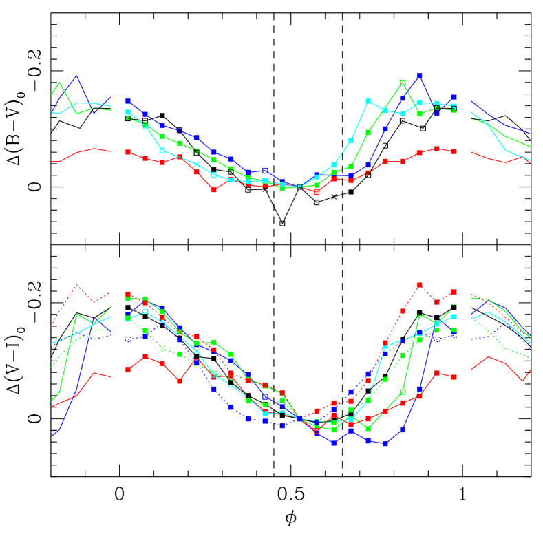
Figure 4: The color curves from Figure 3 shifted vertically to register at $\phi=0.525$.

IV Analysis of Colors

Here we report preliminary results obtained by Tyler Anderson as part of his 2012 M.Sc. thesis. He focused on two definitions of color, the intensity-mean $\langle V\rangle-\langle I\rangle$, and the color at minimum light, $(V-I)_{min}$ using the Sturch (1966) definition of minimum light, $0.5\leq\phi\leq 0.8$ developed for RRab. As shown in the previous section, a phase range of 0.45-0.65 is more appropriate for RRc, so the following results offer only a preliminary look at this relation. Tyler began by correcting each star’s observed color for the small amount of reddening estimated from the reddening maps of Schlegel et al. (1998):

$$(\langle V\rangle-\langle I\rangle)_{0}=(\langle V\rangle-\langle I\rangle)-1.24E(B-V),$$ (2)

with a similar definition for $(V-I)_{min,0}$, and where the color conversion factor of 1.24 is from Cardelli et al. (1989). He then performed leasts-squares regressions of the form

$$(\langle V\rangle-\langle I\rangle)_{0}=c_{0}+c_{1}x,$$ (3)

where $x$ is an independent variable: the pulsation period $P$, the stellar metallicity [Fe/H], or the light curve amplitude, $A_{V}$, taken in turn. For each regression, he computed the rms of the points around the best fit line as a measure of goodness of fit. The results are shown in Table 2 and Figures 5 and 6.

ccccc Preliminary Color Relations for RRc 0pt

Color & $x$ $c_{0}$ $c_{1}$ rms $(\langle V\rangle-\langle I\rangle)_{0}$ & none 0.342 0.000 0.054

$(\langle V\rangle-\langle I\rangle)_{0}$ $P$ 0.036 0.924 0.031

$(\langle V\rangle-\langle I\rangle)_{0}$ [Fe/H] 0.222 –0.074 0.044

$(\langle V\rangle-\langle I\rangle)_{0}$ $A_{V}$ 0.324 0.038 0.054

$(V-I)_{min,0}$ none 0.394 0.000 0.072

$(V-I)_{min,0}$ $P$ 0.225 0.536 0.073

$(V-I)_{min,0}$ [Fe/H] 0.272 –0.086 0.069

$(V-I)_{min,0}$ $A_{V}$ 0.226 0.332 0.059

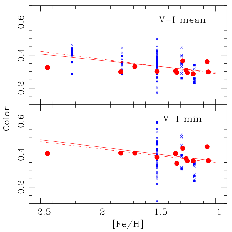
Figure 5: Regressions of $(\langle V\rangle-\langle I\rangle)_{0}$ and $(V-I)_{min,0}$ versus [Fe/H]. Field and cluster stars are shown in red and blue, respectively, with stars having high crowding class marked with crosses. The dashed and solid curves use all the data, and the stars with low crowding class, respectively.

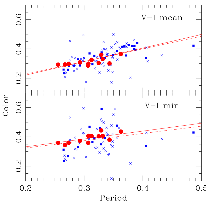
Figure 6: As for Figure 5, but regressed against pulsation period in days.

Figure 5 shows a weak correlation between color and metallicity, with the cluster stars having a marginally steeper slope. Figure 6 shows a stronger correlation between color and period, again with the cluster stars having a marginally steeper slope. Plots of the residuals from this fit versus metallicity and amplitude show little or no slope, indicating that period and metallicity are themselves related. Expanding the model to a color-period-metallicity is thus not warranted. Plots of color versus amplitude, $A_{V}$ show little correlation.

V Conclusions and Future

Our best, preliminary predictor of the intrinsic color of RRc variables is

$$(\langle V\rangle-\langle I\rangle)_{0}=0.036+0.924P,$$ (4)

with rms = 0.031 mag. This scatter is only slightly larger than the best relation for RRab stars from Guldenschuh et al. (2005), indicating that RRc are also valuable tools for measuring interstellar reddening. We show that the cluster and field RRc obey approximately the same relation, further extending the utility of RRc as a reddening indicator.

In the summer of 2013, undergraduate student Paul Husband is working to refine and extend these relations by adding more field and cluster stars, particularly at the metal-poor end of the relation. He is revising the minimum-light color measurements using the more appropriate phase range of 0.45-0.65, and is extending Tyler’s work in $V-I$ to $B-V$ using all three color definitions. We will also use the compiled data to see whether the color changes for stars exhibiting the Blazhko effect when they are observed at different phases in their Blazhko cycles.

Acknowledgements: P.H. and A.C.L. acknowledge support from BGSU’s SETGO Summer Research program, which is funded by the NSF.

References

- Blanco (1992) Blanco, V. M. 1992, AJ, 104, 734
- Benkő et al. (2006) Benkő, J. M., Bakos, G. A., & Nupsl, J. 2006, MNRAS, 372, 1657
- Cardelli et al. (1989) Cardelli, J. A., Clayton, G. C., & Mathis, J. S. 1989, ApJ, 345, 245
- Day et al. (2002) Day, A. S., Layden, A. C., et al. 2002, PASP, 114, 645
- Guldenschuh et al. (2005) Guldenschuh, K. A., Layden, A. C., et al. 2005, PASP, 117, 721
- Harris (1996) Harris, W. E. 1996, AJ, 112, 1478
- Kunder et al. (2010) Kunder, A., Chaboyer, B. & Layden, A. C. 2010, AJ, 139, 415
- Landolt (1992) Landolt, A. U. 1992, AJ, 104, 340
- Mateo et al. (1995) Mateo, M., Udalski, A., Szymanski, M., Kaluzny, J., Kubiak, M., & Krzeminski, W. 1995, AJ, 109, 588
- McNamara (2011) McNamara, B. 2011, AJ, 142, 110
- Preston (1964) Preston, G. W. 1964, ARAA, 2, 23
- Pritzl et al. (2003) Pritzl, B.J., Smith, H.A., Stetson, P.B., Catelan, M., Sweigart, A.V., Layden, A.C., & Rich, R.M. 2003, AJ, 126, 1381
- Reid (1996) Reid, N. 1996, MNRAS, 278, 367
- Sarajedini et al. (2006) Sarajedini, A., Barker, M.K., Geisler, D., Harding, P. & Schommer, R. 2006, AJ, 132, 1361
- Schlegel et al. (1998) Schlegel, D. J., Finkbeiner, D. P., & Davis, M. 1998, ApJ, 500, 525
- Smith (1995) Smith, H. A. 1995, “RR Lyrae Stars,” Cambridge Univ. Press: Cambridge
- Stetson (2000) Stetson, P. B. 2000, PASP, 112, 925
- Stetson et al. (2003) Stetson, P. B., Bruntt, H. & Grundahl, F. 2003, PASP, 115, 41
- Stetson et al. (2005) Stetson, P. B., Catelan, M. & Smith, H. A. 2005, PASP, 117, 1325
- Sturch (1966) Sturch, C. 1966, ApJ, 143, 774
- Walker (1990) Walker, A. R. 1990, AJ, 100, 1532
- Walker (1994) Walker, A. R. 1994, AJ, 108, 555
- Walker (1998) Walker, A. R. 1998, AJ, 116, 220