The Universal Stellar Mass–Stellar Metallicity Relation for Dwarf Galaxies

Abstract

We present spectroscopic metallicities of individual stars in seven gas-rich dwarf irregular galaxies (dIrrs), and we show that dIrrs obey the same mass–metallicity relation as the dwarf spheroidal (dSph) satellites of both the Milky Way and M31: $Z_{*}\propto M_{*}^{0.30\pm 0.02}$. The uniformity of the relation is in contradiction to previous estimates of metallicity based on photometry. This relationship is roughly continuous with the stellar mass–stellar metallicity relation for galaxies as massive as $M_{*}=10^{12}~{}M_{\sun}$. Although the average metallicities of dwarf galaxies depend only on stellar mass, the shapes of their metallicity distributions depend on galaxy type. The metallicity distributions of dIrrs resemble simple, leaky box chemical evolution models, whereas dSphs require an additional parameter, such as gas accretion, to explain the shapes of their metallicity distributions. Furthermore, the metallicity distributions of the more luminous dSphs have sharp, metal-rich cut-offs that are consistent with the sudden truncation of star formation due to ram pressure stripping.

1. Introduction

The average metal content of a galaxy correlates with its mass. More massive galaxies are more metal-rich than less massive galaxies. The relation can be explained by the retention of metals in the galaxies’ gravitational potential wells (e.g., Dekel & Silk, 1986). High-mass galaxies have deep potential wells that can resist some of the expulsion of gas and metals by supernova winds, stellar winds, and galaxy-scale feedback. Low-mass galaxies lack the gravity to resist these feedback mechanisms. The correlation between metallicity and mass can also be explained by a correlation between star formation efficiency and stellar mass (e.g., Matteucci, 1994; Calura et al., 2009; Magrini et al., 2012; Pipino et al., 2013). If massive galaxies evolve quickly, then they can achieve high stellar masses and low gas mass fractions. Consequently, their metallicities will be high. On the other hand, slowly evolving, low-mass galaxies can have high gas fractions, which dilute the metallicity of both the gas and the stars that form from the gas. Yet another explanation for the mass–metallicity relation is a stellar initial mass function (IMF) that changes with the rate of star formation (Köppen et al., 2007). Because that rate depends on galaxy mass and because the metal yield depends on the masses of stars, a galaxy’s metallicity then depends on its stellar mass.

Galactic metallicity is typically measured in the gas phase. Emission line diagnostics of metallicity (e.g., Kewley & Dopita, 2002) sample the metallicity of H II regions. Hence, these measures probe presently star-forming gas. Using strong line diagnostics, McClure & van den Bergh (1968) and Lequeux et al. (1979) established the first luminosity–metallicity relations (LZRs) for star-forming galaxies. Lequeux et al. found that the effective metal yields of all of the galaxies they considered were below the true yield expected from a “closed box” or “simple” model of galactic chemical evolution (Schmidt, 1963; Talbot & Arnett, 1971; Searle & Sargent, 1972). More recently, Tremonti et al. (2004) showed that the average metallicities of star-forming galaxies in the Sloan Digital Sky Survey (SDSS, Abazajian et al., 2004) correlate strongly with their stellar masses or rotation speeds. The correlation with stellar mass has an intrinsic scatter of only 0.1 dex in $\log({\rm O/H})$. As with previous studies, Tremonti et al. interpreted the relation as a progression of a larger effective yield for more massive galaxies. Expressed another way, more massive galaxies lose a smaller fraction of the metals that their stars produce.

The mass–metallicity relation (MZR)—where metallicity was measured in the gas phase—extends down to the mass range of dwarf galaxies as small as a few million solar masses. Mould et al. (1983) and Skillman et al. (1989) showed that dwarf elliptical (dE) and dwarf irregular galaxies (dIrrs) in and around the Local Group (LG) obey a LZR. Garnett (2002) extended the relation to more distant spiral galaxies. Irregular and spiral galaxies obey the same, unbroken relation over 4.5 orders of magnitude in luminosity.

One of the sources of error in determining the MZR is the stellar mass-to-light ratio ($M_{*}/L$). This ratio is required to convert the LZR into the MZR. It depends on a galaxy’s star formation history (SFH) with potential contributions from the stellar IMF. Lee et al. (2006a) measured stellar masses for dwarf galaxies based on 4.5 $\mu$m luminosity, which is less sensitive to age, SFH, and dust than visible luminosity. While Skillman et al. (1989) already established that the LZR applies to dwarf galaxies, Lee et al. (2006a) showed that the MZR from more massive spiral galaxies (Tremonti et al., 2004) also applies to dIrrs.

The MZR also exists at high redshift. Erb et al. (2006) found that the relation persists, but evolves in the sense that high-redshift galaxies are more metal-poor at a given stellar mass than galaxies in the local universe. Zahid et al. (2013) and Henry et al. (2013) showed that the MZR evolves smoothly from $z=2.2$ to the present. However, Mannucci et al. (2010), Hunt et al. (2012), and Lara-López et al. (2013) found that the independent variable controlling the offset of the MZR was star formation rate (SFR), not redshift. Because SFR increases with redshift (Madau et al., 1996), it appeared as though the MZR was evolving, but it is in fact constant after the correction for SFR. Correcting for SFR leads to the unevolving “fundamental metallicity relation.” Star formation depresses the gas-phase metallicity of a galaxy because star formation requires hydrogen gas. Metallicity is expressed as the ratio of metals to hydrogen. Therefore, vigorously star forming galaxies contain a lot of hydrogen, which dilutes the metals. In fact, Bothwell et al. (2013) established that the offset in the MZR correlates better with H I gas mass than SFR.

The majority of stellar mass in the local universe resides in galaxies that are not forming stars and have very little gas (Bell et al., 2003; Baldry et al., 2004; Gallazzi et al., 2008). Therefore, it is not possible to place them on the same fundamental metallicity relation corrected for SFR or gas mass. Instead, it is necessary to construct a separate MZR that measures stellar metallicity rather than gas-phase metallicity.

Emission line diagnostics of metallicity apply only to star-forming galaxies. They sample the present metallicity of stars forming at the time of observation. A complementary technique for measuring the composition of a galaxy is to measure stellar metallicities from stellar colors or spectral absorption lines. Baum (1959) first noticed a correlation between galaxies’ $B-V$ colors and their absolute magnitudes. He suggested that the cause of the correlation was a variable ratio of Population I (young, metal-rich) to Population II (old, metal-poor) stars. In essence, he first suggested the idea of a LZR. Later, Sandage & Visvanathan (1978) showed that the color–magnitude relation applies to both Virgo cluster galaxies and field galaxies.

The stellar metallicity of a galaxy is a record of the past star formation. Each star preserves the metallicity of the galactic gas at the time and site of formation. A stellar metallicity distribution function is therefore a chronicle of the chemical evolution of the galaxy. In the typical mode of a monotonic increase of gas metallicity with time, the gas-phase metallicity is greater than the average stellar metallicity. Furthermore, the gas-phase metallicity in principle fluctuates more than the stellar metallicity. The gas metallicity changes as rapidly as gas flows into and out of the galaxy, whereas the stellar metallicity responds to gas flows on a longer timescale, which depends on the SFR. On the other hand, Berg et al. (2011, 2012) showed that the dispersion in the MZR is just 0.15 dex when the “direct” method is used to measure gas-phase abundances from auroral lines. Furthermore, rare outliers from the MZR when using the strong nebular lines are not outliers when using the more trusted, direct method. The low dispersion leaves little room for large fluctuations in the gas-phase metallicity. However, the direct method is only practical for a limited range of galaxies because the [O III] $\lambda$4363 emission line is intrinsically faint, especially at high metallicities ($12+\log({\rm O/H})\gtrsim 8.5$).

Quiescent and gas-free galaxies have no emission lines. The only light from these galaxies comes from stars. Hence, spectroscopic metallicities must be measured from absorption lines rather than emission lines. In practice, models of the integrated light spectrum from an entire stellar population (Tinsley & Gunn, 1976) are compared to observed galaxy spectra. One implementation of this technique is to measure spectrophotometric indices, such as Lick indices (Faber, 1973; Worthey, 1994). Bruzual & Charlot (2003) updated the use of line indices to rely on spectral models rather than fixed-resolution templates. This method can even be used with ultraviolet line indices for high-redshift galaxies (Rix et al., 2004; Halliday et al., 2008; Sommariva et al., 2012). Spectral models can even be compared directly to observed spectra without compressing the abundance information into a few line indices (e.g., Conroy et al., 2009). Gallazzi et al. (2005) applied the Bruzual & Charlot models to SDSS spectra of over 40,000 galaxies. They showed that the average stellar metallicities of galaxies with stellar masses in the range $10^{9}<M_{*}/M_{\sun}<10^{12}$ correlate tightly with stellar mass. The correlation has the same shape as the correlation between gas-phase metallicity and stellar mass for SDSS galaxies found by Tremonti et al. (2004). Gallazzi et al. (2006) showed that early-type galaxies’ stellar metallicities correlate better with their dynamical masses than their stellar masses. The correlation with dynamical mass lends credence to the theory that galaxies with shallower potential wells are more susceptible to metal loss.

On the other hand, dark matter halo masses for dwarf galaxies ($M_{*}<10^{8}~{}M_{\sun}$) may not correlate at all with their stellar masses or metallicities (Strigari et al., 2008). However, the full dark matter potential is difficult to measure in any galaxy. While it is straightforward to constrain the mass within the half-light radius (Wolf et al., 2010), it is nearly impossible to measure the total gravitational potentials of most dispersion-supported galaxies in the absence of an extended tracer (Tollerud et al., 2011). The baryons are so deeply embedded in the dark matter halo that any connection to halo virial mass requires a theoretical extrapolation.

Gas-phase abundances are usually expressed in terms of oxygen abundance. Oxygen absorption lines in stars are few and weak. The spectral features most readily available in stars are from iron and magnesium. Therefore, comparing gas-phase to stellar metallicities requires the assumption of abundance ratios, such as [O/Fe]. This ratio depends on the SFH. Another option to compare gas-phase abundances in star-forming galaxies to quiescent galaxies is to measure oxygen abundances of planetary nebulae (PNe), which are the long-lived remnants of dead stars. Richer & McCall (1995) measured the oxygen abundances of PNe in both dIrrs and dwarf elliptical/spheroidal galaxies (dEs/dSphs). They found that the dE/dSph LZR was offset from dIrrs in the sense that PNe in dEs and dSphs are more oxygen-rich than in dIrrs of similar luminosity. There is some question about whether oxygen abundances in PNe trace the oxygen abundances of stars. Richer et al. (1998) laid out the reasons for possible discrepancies, but did not find them to apply to the PNe in dwarf galaxies. Gonçalves et al. (2007) revisited the offset, and they showed that it applies whether the oxygen abundances in dIrrs are measured from PNe or H II regions. One possibility is that the PNe themselves produce oxygen in the third dredge-up, while they are expelling their envelopes (e.g., Magrini et al., 2005). Another possibility is that PNe and H II regions could preferentially trace a younger, more metal-rich population than the average.

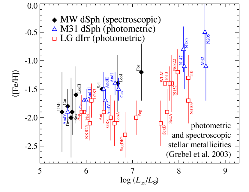
Figure 1.— The luminosity–stellar metallicity relation for Local Group dwarf galaxies where the metallicity is determined from spectroscopy (filled symbols) and photometry (hollow symbols). The data is taken from the compilation of Grebel et al. (2003). There is an apparent offset between dIrrs and dSphs. We argue that the offset is not a reflection of the dIrrs’ true metallicities and is instead caused by the age–metallicity degeneracy for photometric metallicities.

Nearby galaxies can be resolved into individual H II regions and individual stars. Whereas integrated light spectra do not allow a measurement of the spread of metallicity within a galaxy, spectroscopy of individual stars resolves the shapes of metallicity distributions. Individual stellar metallicities can be measured from color–magnitude diagrams (CMDs). Grebel et al. (2003) compiled average metallicities of LG dwarf galaxies. The metallicities were measured spectroscopically for the nearer dSph galaxies and from the optical colors of the red giant branch (RGB) for the more distant dIrr galaxies. In agreement with the oxygen measurements from PNe, Grebel et al. (2003) found an offset in the LZR such that dIrrs are more iron-poor at fixed luminosity than dSphs (see Figure 1).

However, the colors of red giants are subject to the age–metallicity degeneracy (e.g., Salaris & Girardi, 2005; Lianou et al., 2011). As a stellar population ages, the RGB becomes redder. However, more metal-rich red giants are also redder. Thus, the age of the population needs to be determined before the RGB color can be used to measure metallicity. Determining the age is especially important for a comparison between dSphs and dIrrs because the stellar populations of dSphs are systematically older than dIrrs. Lee et al. (2008) reported in conference proceedings that they re-analyzed the metallicities of dIrrs from RGB colors, and they found iron metallicities on average 0.5 dex higher than Grebel et al. (2003) for the same galaxies. The difference in the analyses arose from a different treatment in the ages of the stellar populations as well as accounting for a spread in age and metallicity. The offset between dIrrs and dSphs in the LZR vanished in the more recent study.

When it is possible to observe stars spectroscopically, spectroscopic metallicities are preferred to photometric metallicities because the age–metallicity degeneracy applies only in subtle ways to stellar spectra. Armandroff & Da Costa (1991) first measured the spectroscopic metallicities for extragalactic stars. They based their measurements of the Carina dSph on the strength of the near-infrared Ca II triplet (CaT), which they calibrated to Galactic globular clusters of known metallicity. Since then, the CaT technique has been used to quantify the metallicity distributions of most of the classical dSph Milky Way (MW) satellites (e.g., Helmi et al., 2006) and two dIrrs: NGC 6822 (Tolstoy et al., 2001) and WLM at a distance of 930 kpc (Leaman et al., 2009). Using a technique not based on empirical calibrations, Kirby et al. (2008b, 2011a) quantified the metallicity distributions of 15 MW dSphs using synthetic spectral fitting to iron lines in individual red giants. They found a single, power-law relation between metallicity and galaxy luminosity over the range $10^{3.5}<L/L_{\sun}<10^{7.3}$. This relation for dSphs is consistent with the MZR determined from photometric metallicities of stars in more massive dEs (Grebel et al., 2003; Woo et al., 2008).

In the present study, we extend our spectroscopic analysis of iron lines in red giants to gas-rich dIrrs. We aim to resolve the ambiguity of the photometric metallicity measurements in dIrrs. We construct a unified stellar mass–stellar metallicity relation for LG dwarf galaxies of various morphologies, ages, and gas fractions. This relation spans six orders of magnitude in luminosity or stellar mass. We further connect this relation to the stellar mass–stellar metallicity relation of more massive galaxies (Gallazzi et al., 2005). We discuss the origin of the universal MZR in the context of metal loss. Finally, we present the shapes of the metallicity distributions and discuss the role of gas inflow, outflow, and ram pressure stripping.

2. Spectroscopic Observations

2.1. The Galaxy Sample

Table 1Dwarf Galaxy Sample

Galaxy	RA (J2000)	Dec (J2000)	$\log M_{*}$	$D_{\rm MW}$	$D_{\rm M31}$	$v_{\rm rot}/\sigma_{v}$	$M_{\rm HI}/M_{*}$
			($M_{\sun}$)	(kpc)	(kpc)
Milky Way dSphs
Fornax	02 39 59	$-$34 26 57	7.39	0149	$\cdots$	$<1$	0
Leo I	10 08 28	$+$12 18 23	6.69	0258	$\cdots$	$<1$	0
Sculptor	01 00 09	$-$33 42 33	6.59	0086	$\cdots$	$<1$	0
Leo II	11 13 29	$+$22 09 06	6.07	0236	$\cdots$	$\cdots$	0
Sextans	10 13 03	$-$01 36 53	5.84	0089	$\cdots$	$<1$	0
Ursa Minor	15 09 08	$+$67 13 21	5.73	0078	$\cdots$	$<1$	0
Draco	17 20 12	$+$57 54 55	5.51	0076	$\cdots$	$<1$	0
Canes Venatici I	13 28 04	$+$33 33 21	5.48	0218	$\cdots$	$\cdots$	0
Hercules	16 31 02	$+$12 47 30	4.57	0126	$\cdots$	$\cdots$	0
Ursa Major I	10 34 53	$+$51 55 12	4.25	0102	$\cdots$	$\cdots$	0
Leo IV	11 32 57	$-$00 32 00	3.93	0155	$\cdots$	$\cdots$	0
Canes Venatici II	12 57 10	$+$34 19 15	3.90	0161	$\cdots$	$\cdots$	0
Ursa Major II	08 51 30	$+$63 07 48	3.73	0038	$\cdots$	$<1$	0
Coma Berenices	12 26 59	$+$23 54 15	3.68	0045	$\cdots$	$<1$	0
Segue 2	02 19 16	$+$20 10 31	3.01	0041	$\cdots$	$\cdots$	$\cdots$
Local Group dIrrs
NGC 6822	19 44 56	$-$14 47 21	7.92	0452	0897	8.1	1.6
IC 1613	01 04 48	$+$02 07 04	8.01	0758	0520	4.2	0.6
VV 124	09 16 02	$+$52 50 24	7.00	1367	1395	$<1$	0.1
Pegasus dIrr	23 28 36	$+$14 44 35	6.82	0921	0474	$>2.3$	0.9
Leo A	09 59 27	$+$30 44 47	6.47	0803	1200	$<1$	3.7
Aquarius	20 46 52	$-$12 50 53	6.15	1066	1173	$<1$	2.9
Leo T	09 34 53	$+$17 03 05	5.21	0422	0991	$<1$	1.7
M31 dSphs
NGC 205	00 40 22	$+$41 41 07	8.67	$\cdots$	0042	0.3	0.0009
NGC 185	00 38 58	$+$48 20 15	7.83	$\cdots$	0187	0.6	0.0016
NGC 147	00 33 12	$+$48 30 32	8.00	$\cdots$	0142	1.1	0
Andromeda VII	23 26 32	$+$50 40 33	6.93	$\cdots$	0218	$\cdots$	0
Andromeda II	01 16 30	$+$33 25 09	6.88	$\cdots$	0184	$\cdots$	0
Andromeda I	00 45 40	$+$38 02 28	6.80	$\cdots$	0058	$\cdots$	0
Andromeda III	00 35 34	$+$36 29 52	6.18	$\cdots$	0075	$\cdots$	0
Andromeda XVIII	00 02 15	$+$45 05 20	5.78	1358	0591	$\cdots$	$\cdots$
Andromeda XV	01 14 19	$+$38 07 03	5.76	$\cdots$	0174	$\cdots$	0
Andromeda V	01 10 17	$+$47 37 41	5.63	$\cdots$	0110	$\cdots$	0
Andromeda XIV	00 51 35	$+$29 41 49	5.45	$\cdots$	0162	$\cdots$	0
Andromeda IX	00 52 53	$+$43 11 45	5.26	$\cdots$	0040	$\cdots$	0
Andromeda X	01 06 34	$+$44 48 16	5.02	$\cdots$	0110	$\cdots$	0

References. — The June 2013 version of the compilation of McConnachie (2012) and references therein.

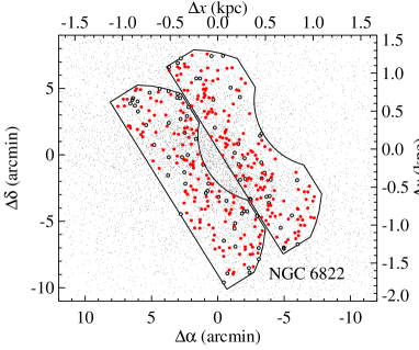
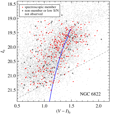
Figure 2.— Stars from the NGC 6822 photometric catalog (Massey et al., 2007) represented in celestial coordinates (left) and in a color–magnitude diagram (right). The irregular shapes in the left panel show the outlines of the DEIMOS field of view for both slitmasks. Solid red and hollow black points show targets for which we obtained DEIMOS spectra. Solid red points are spectroscopically confirmed members. The blue curve in the right panel is a Padova theoretical isochrone (Girardi et al., 2002) with an age of 6 Gyr and a metallicity of ${\rm[Fe/H]}=-1.2$. The age of the isochrone is not meant to indicate the true age of the galaxy. It was chosen merely to illustrate the approximate shape of the RGB. Stars below the dashed gray line have uncertainties in $V_{0}$ larger than 0.1 dex.

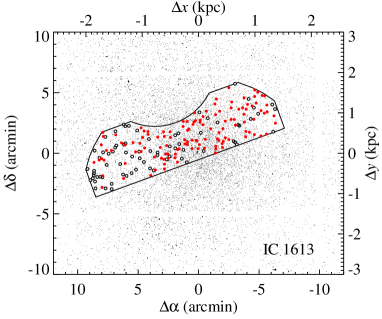
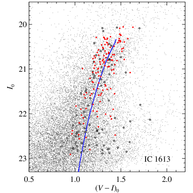
Figure 3.— Stars from the IC 1613 photometric catalog (Bernard et al., 2007). The symbols are the same as in Figure 2. The blue curve is a Padova theoretical isochrone (Girardi et al., 2002) with an age of 4 Gyr and a metallicity of ${\rm[Fe/H]}=-1.2$.

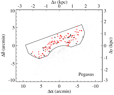
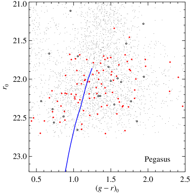
Figure 4.— Stars from the SDSS DR7 catalog (Abazajian et al., 2009) centered on the Pegasus dIrr. Substantial photometric errors blur the shape of the RGB. The symbols are the same as in Figure 2. The blue curve is a Padova theoretical isochrone (Girardi et al., 2004) with an age of 12 Gyr and a metallicity of ${\rm[Fe/H]}=-1.2$.

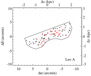
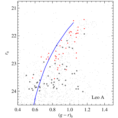
Figure 5.— Stars from the Leo A photometric catalog (McMahon et al., 2001). The symbols are the same as in Figure 2. The blue curve is a Padova theoretical isochrone (Girardi et al., 2004) with an age of 8 Gyr and a metallicity of ${\rm[Fe/H]}=-1.6$. Although the isochrone is bluer than most of the stars, an older, redder isochrone would be inconsistent with the photometrically measured SFH (Cole et al., 2007).

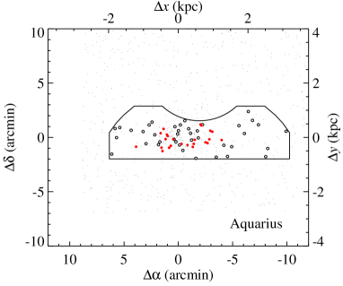
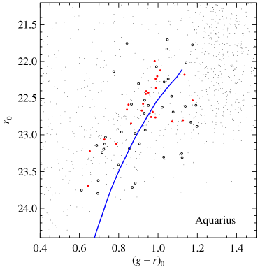
Figure 6.— Stars from the Aquarius photometric catalog. The symbols are the same as in Figure 2. The blue curve is a Padova theoretical isochrone (Girardi et al., 2004) with an age of 2 Gyr and a metallicity of ${\rm[Fe/H]}=-1.2$.

Table 2DEIMOS Observations of dIrrs

Galaxy	Slitmask	# targets	Exp. Time	Date			Seeing	Individual Exposures
			(h)	(UT)			(′′)	(s)
NGC 6822	n6822a	180	08.7	2010	Aug	12	$1.2$	$5\times 1800+1630+1560+1200$
				2011	Jul	30	$0.7$	$2\times 1800$
				2011	Jul	31	$0.7$	$5\times 1800$
				2011	Aug	6	$1.0$	$3\times 1800$
	n6822b	180	06.0	2011	Jul	29	$0.7$	$8\times 1800$
				2011	Aug	4	$0.9$	$4\times 1800$
IC 1613	i1613a	199	10.3	2010	Aug	11	$0.9$	$5\times 1800+2\times 1500$
				2010	Aug	13	$0.9$	$3\times 1800+720$
				2011	Jul	29	$0.7$	$2\times 1800+2\times 1680$
				2011	Jul	30	$0.7$	$3\times 1800+1020$
				2011	Jul	31	$0.7$	$3\times 1800$
VV 124	vv124a	121	03.7	2011	Jan	30	$0.6$	$6\times 1800+2\times 1200$
	vv124b	120	03.8	2011	Jan	30	$0.6$	$6\times 1800+1600+1200$
Pegasus dIrr	pega	113	06.8	2011	Aug	4	$0.7$	$1800+1680+1380+600$
				2011	Aug	5	$0.9$	$2\times 1800+2\times 1500+1200$
				2011	Aug	6	$1.0$	$1800+1720+600$
				2011	Aug	7	$0.4$	$1800+3\times 1500+900$
Leo A	leoaaW	091	06.7	2013	Jan	14	$0.9$	$12\times 1800+2\times 1200$
Aquarius	aqra	064	08.9	2013	Jul	8	$0.5$	$10\times 1800+1260+720$
				2013	Sep	1	$0.7$	$2\times 1800$
				2013	Sep	2	$0.9$	$3\times 1800+2\times 1560$
Leo T	LeoT–1	087	01.0	2007	Feb	14	$0.7$	$3\times 1200$

We observed dwarf galaxies spanning a range of luminosities and galaxy types. In order to maintain the homogeneity of the spectroscopic data by using only Keck/DEIMOS (Faber et al., 2003) spectroscopy, we observed only galaxies visible from Mauna Kea. Table 2.1 lists the galaxies observed, separated by host (MW or M31) and galaxy type (dSph/dE or dIrr). The table includes the primary observables that distinguish dSphs from dIrrs (the June 2013 version of the compilation of McConnachie, 2012, and references therein).

DSphs and dEs are distinct from dIrrs in their morphology; distance from a host galaxy, like the MW or M31; degree of rotation, quantifiable as the ratio of the rotation speed to the velocity dispersion ($v_{\rm rot}/\sigma_{v}$); and gas content. The distinction between dSphs and dEs is not clear. The two classes have similar surface brightness profiles, which are distinct from slightly larger “true” elliptical galaxies, like M32 (Wirth & Gallagher, 1984; Kormendy et al., 2009). The dEs of M31 (NGC 147, 185, and 205) seem to be higher luminosity counterparts to LG dSphs. Therefore, we classify those three galaxies as dSphs.

On the other hand, the dIrrs are not a homogeneous group. Some dIrrs, like VV 124, Pegasus, and Leo T, share some properties with dSphs. Their stellar and gas motions may be less dominated by rotation than dispersion, and they may have lower gas fractions than typical dIrrs. In accordance with the theory that dIrrs transform into dSphs by interaction with a larger galaxy (Lin & Faber, 1983; Mayer et al., 2001), these galaxies are called transition dwarf galaxies (dTs or dIrr/dSphs). Alternatively, at least some dTs may simply be dIrrs that are experiencing a temporary lull in SFR (Skillman et al., 2003), but the morphology–density relation indicates that proximity to a host plays some role in making the transition from dSph to dIrr (Weisz et al., 2011). However, even dTs are starkly distinct from dSphs, especially in their gas fractions. All of the dSphs in our sample have $M_{\rm HI}/M_{*}<0.002$ and all of the dIrrs and dTs have $M_{\rm HI}/M_{*}\geq 0.1$. For simplicity, we conflate dIrrs and dTs into a single category called dIrr.

Much of the spectroscopy and chemical analysis presented here has already been published. Simon & Geha (2007) and Kirby et al. (2010, 2013) published the details of the observations and the analysis of the MW dSphs. Simon & Geha also included the Leo T transition dwarf galaxy in their sample. Kirby et al. (2012) described the VV 124 data and analysis. The M31 satellite sample comes from the Spectroscopic and Panchromatic Landscape of Andromeda’s Stellar Halo (SPLASH, Guhathakurta et al., 2005, 2006). The details of the spectroscopy have been published by Geha et al. (2006, 2010, NGC 147, 185, and 205), Kalirai et al. (2009, 2010, Andromeda I, II, III, VII, and X), Ho et al. (2012, additional Andromeda II spectra), Majewski et al. (2007, Andromeda XIV), and Tollerud et al. (2012, Andromeda V, IX, XV, and XVIII and additional spectroscopy of Andromeda III and XIV).

We present new spectroscopy of red giants in NGC 6822, IC 1613, the Pegasus dIrr, Leo A, and Aquarius. These are the first published results from red giant spectroscopy in all of these galaxies except NGC 6822, which was studied by Tolstoy et al. (2001). The next section describes our target selection for the new spectroscopy.

2.2. Target Selection

We selected red giants for DEIMOS spectroscopy from existing photometric catalogs of NGC 6822, IC 1613, Pegasus, and Leo A. We obtained new images of Aquarius with Subaru/Suprime-Cam (Miyazaki et al., 2002).

2.2.1 NGC 6822

We selected targets in NGC 6822 from Massey et al.’s (2007) $UBVRI$ photometric catalog. The NGC 6822 data came from the Mosaic camera on the Cerro Tololo Blanco 4 m telescope. RGB candidates were selected from the CMD assuming a distance modulus of 23.40, based on measurements of Cepheid variables (Feast et al., 2012). No star with an apparent magnitude fainter than $I=22$ was selected. Magnitudes were corrected for extinction based on a reddening of $E(B-V)=0.25$ (Massey et al., 2007). In order not to bias the sample with respect to metallicity, color was not given much weight in the target selection other than to select targets with the approximate colors of red giants. Figure 2 shows the target selection in celestial coordinates and in a CMD. The figure also identifies targets that passed the spectroscopic membership criteria (Section 3.1). The theoretical isochrones shown in Figure 2 and in the subsequent figures are meant simply to show the approximate shape of the RGB, not to indicate the true ages of the galaxies.

2.2.2 IC 1613

We selected DEIMOS targets for IC 1613 from Bernard et al.’s (2007) photometric catalog, kindly provided to us by E. Bernard. We assumed a Cepheid-based distance modulus of 24.34 (Tammann et al., 2011). The faint magnitude limit was $I=23$. The extinction corrections were $A_{V}=0.08$ and $A_{I}=0.05$ (Sakai et al., 2004). Other details are the same as NGC 6822. Figure 3 shows the target selection.

2.2.3 Pegasus dIrr

We consulted SDSS Data Release 7 (DR7, Abazajian et al., 2009) to generate a photometric catalog for Pegasus. We used CasJobs, the SDSS database server, to download $ugriz$ magnitudes for all point sources classified as stars within $30^{\prime}$ of Pegasus. The tip of the RGB in Pegasus is close to SDSS’s faint magnitude limit. As a result, the photometric errors are large, as revealed by the large scatter of spectroscopic targets in color and magnitude (Figure 4). The Cepheid-based distance modulus is 24.87 (Tammann et al., 2011). We used SDSS’s extinction corrections, which are based on the Schlegel et al. (1998) dust maps. The faint magnitude limit, set by the SDSS photometric depth, was $r=23$.

2.2.4 Leo A

We selected spectroscopic targets in Leo A from the Isaac Newton Telescope Wide Field Survey (McMahon et al., 2001). A. Cole and M. Irwin kindly provided the photometric catalog to us. We imposed a faint magnitude limit of $r=24.1$. We assumed the Cepheid-based distance of 24.59 (Tammann et al., 2011). We corrected for extinction star by star based on the Schlegel et al. (1998) dust maps. Other details are the same as NGC 6822. Figure 5 shows the targets.

2.2.5 Aquarius

We observed Aquarius with Suprime-Cam on 2010 May 25 in $0.8^{\prime\prime}$ seeing. We obtained five 60 s exposures in each of the $g$ and $r$ filters for a total of five minutes in each filter. The images were reduced with the SDFRED2 software (Ouchi et al., 2004). We identified point sources and calculated photometric magnitudes using DAOPHOT (Stetson, 1987) within version 2.12.2 of IRAF (Tody, 1986).

We selected targets for spectroscopy in a manner similar to the other dIrrs. The assumed distance modulus, based on the magnitude of the tip of the RGB, was 25.15 (McConnachie et al., 2006). We imposed a faint magnitude limit of $r=24$. We corrected magnitudes for extinctions of $A_{g}=0.20$ and $A_{r}=0.13$ (Schlegel et al., 1998). Figure 6 shows the astrometry and photometry for spectroscopic targets.

2.3. DEIMOS Spectroscopy

We observed the new dIrr slitmasks with DEIMOS in the summers of 2010, 2011, and 2013. We observed two slitmasks for NGC 6822 and VV 124 and one slitmask each for the remaining dIrrs. Table 2 gives the number of red giant candidates, the exposure time, the observation date, and the seeing for each slitmask.

We configured the spectrograph in the same way for all of the slitmasks. We used the 1200G grating, which has a groove spacing of 1200 mm^-1 and a blaze wavelength of 7760 Å. The grating was tilted to a central wavelength of 7800 Å, which resulted in a spectral range of roughly 6400–9000 Å. The exact spectral range for each object depended on the placement of the slit on the slitmask. The slit width was $0.7^{\prime\prime}$ for all slitmasks except leoaaW. For Leo A, we used a backup slitmask with $1.1^{\prime\prime}$ slits because the seeing exceeded $1^{\prime\prime}$ when we started observing. The resolution of DEIMOS in this configuration yields a line profile of 1.2 Å FWHM for the $0.7^{\prime\prime}$ slits and 1.8 Å FWHM for the $1.1^{\prime\prime}$ slits. These resolutions correspond to resolving powers of $R\sim 7100$ and 4700, respectively, at 8500 Å, near the CaT. We reduced the data into sky-subtracted, one-dimensional spectra with the spec2d software pipeline (Cooper et al., 2012; Newman et al., 2013). For slightly more details on the observing and reduction procedures, see Kirby et al. (2012).

3. Metallicity Measurements

3.1. Membership

We removed contaminants that do not belong to the galaxies from the spectroscopic sample in order to have clean metallicity distributions. We imposed membership cuts based on the CMD, spectral features, and radial velocities.

The CMD membership cut was very lax. Stars that could plausibly be members of the RGB in each galaxy were allowed. No culling based on the CMD was performed after the slitmasks were designed. This liberalism with color selection minimizes selection bias in the metallicity distribution (but see Section 3.4). The selection of stars based on colors and magnitudes is shown in Figures 2 through 6.

The membership cut based on spectral features was also not stringent. We discarded a few stars with very strong Na I 8190 doublets, which happen only in dwarf stars with high surface gravities (Spinrad & Taylor, 1971). All of these stars would also have been ruled non-members on the basis of radial velocity.

The primary membership cut was radial velocity. We used the same procedure for determining velocity membership as Kirby et al. (2010). The radial velocities were measured by cross-correlating the observed spectra with DEIMOS template spectra in the wavelength range of the CaT. We used the same templates as Simon & Geha (2007). For each galaxy, we started with a guess at the average velocity ($v_{0}$) and velocity dispersion ($\sigma_{v}$). Then, we discarded all stars more than $3\sigma_{v}$ discrepant from $v_{0}$. We recalculated $v_{0}$ and $\sigma_{v}$ from the culled sample, and we repeated the process until it converged. The stars in each galaxy that passed this iterative membership cut comprise the final member samples.

3.2. Individual Stellar Metallicities

We measured spectroscopic metallicities for individual stars in the dIrrs and the MW satellites. Kirby et al. (2008b, 2009, 2010, 2012, 2013) published the metallicities for the MW satellites, VV 124, and Leo T. Here, we present new measurements for the remaining dIrrs.

Kirby et al. (2008a, 2009, 2010) detailed the technique for measuring metallicities for individual stars. It is based on spectral synthesis of Fe I absorption lines. First, the continuum of the observed spectrum was shifted to the rest frame and normalized to unity. Then, it was compared to a large grid of synthetic spectra. The search for the best-fitting synthetic spectrum was a minimization of $\chi^{2}$ of pixels around Fe I lines.

Photometry helped to constrain the surface gravity and effective temperature. The surface gravity was fixed with the help of 14 Gyr theoretical isochrones and the observed color and magnitude of the star. The same method was used to determine a first guess at the effective temperature, but the temperature was allowed to vary during the spectral fitting within a range around the photometric temperature. The amount by which the spectroscopic temperature was allowed to stray from the photometric temperature depended on the magnitude of the error in the photometric color. For galaxies with photometry in the Johnson/Cousins filter set, we used Yonsei-Yale isochrones (Demarque et al., 2004). For photometry in the SDSS filter set, we used Padova isochrones (Girardi et al., 2004), which were computed with SDSS filter transmission curves. This procedure is slightly different from our earlier metallicity catalogs (Kirby et al., 2008b, 2010), where we transformed SDSS magnitudes to Johnson/Cousins magnitudes. As a result, some of the average metallicities for galaxies are slightly different, especially for the ultra-faint galaxies (Kirby et al., 2008b). We made this revision to eliminate any potential errors caused by the transformation of colors.

After the best-fitting temperature and metallicity were found, the [$\alpha$/Fe] ratio was measured from neutral Mg, Si, Ca, and Ti lines. Next, the metallicity measurement was refined based on the measured [$\alpha$/Fe] ratio. The process was repeated until neither [Fe/H] nor [$\alpha$/Fe] changed between iterations. Finally, [Mg/Fe], [Si/Fe], [Ca/Fe], and [Ti/Fe] were measured individually. This paper presents measurements of [Fe/H] only. The [$\alpha$/Fe] ratios will be used in a different study of the SFHs of the dIrrs, similar to Kirby et al.’s (2011b) study of the SFHs of the MW dSph satellites.

We discovered a minor error in the metallicity measurements published by Kirby et al. (2010). The $[\alpha/{\rm Fe}]_{\rm atm}$ ratio sometimes fixed itself on spurious $\chi^{2}$ minima. This error affected the measurement of [Fe/H] by a small amount, on the order of 0.1–0.2 dex. This study includes the corrected measurements.

Table 3 gives the coordinates, extinction-corrected magnitudes, temperatures, gravities, microturbulent velocities, and metallicities for all of the individual member stars in the dIrrs and the MW satellites. The photometric filter set varies from galaxy to galaxy. Table 3 includes Washington $M$ and $T_{2}$ magnitudes; Johnson/Cousins $B$, $V$, $R$, and $I$ magnitudes; and SDSS $g$, $r$, and $i$ magnitudes. The metallicities for the MW satellites have been corrected for the aforementioned error.

3.3. Coadded Stellar Metallicities

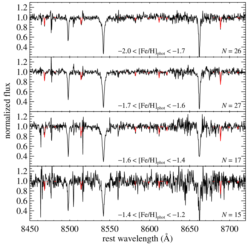
Figure 7.— Small portions of coadded spectra (black) for the four bins of stars in Andromeda V. Portions of the best-fitting, coadded, synthetic spectra that were used for determining [Fe/H] from Fe I lines are shown in red. Each panel gives the photometric metallicity range of the bin and the number of stars in the bin.

The M31 satellite spectra are too noisy to permit metallicity measurements of individual stars. We coadded the spectra in order to attain signal-to-noise ratios (S/Ns) sufficient for comparing to the grid of synthetic spectra. Yang et al. (2013) described this technique and demonstrated that it is effective at recovering the average metallicities for groups of stars. We applied their procedure to the M31 satellite spectra.

The stars were selected for membership based on position in the CMD and radial velocity (see Tollerud et al., 2012). The measurement of velocities does not require S/N as high as the measurement of metallicity. Hence, velocities can be determined for individual stars. These velocities and the associated membership cuts were given by the references listed in Section 2.1.

The binning was based on photometric metallicity (${\rm[Fe/H]}_{\rm phot}$), which was determined by comparing the de-reddened color and extinction-corrected magnitude of each star to a set of theoretical Yonsei–Yale isochrones (Demarque et al., 2004) with an age of 14 Gyr. This choice of age affects the binning but not the spectroscopic metallicity. By interpolating in the CMD between isochrones of different metallicities, a value of ${\rm[Fe/H]}_{\rm phot}$ can be assigned to each star. The stars were binned in ${\rm[Fe/H]}_{\rm phot}$. This procedure is similar to binning by color, but it accounts for the curvature of the RGB in the CMD. The bins were chosen to have a minimum width of $\Delta{\rm[Fe/H]}_{\rm phot}=0.1$ and a minimum of 15 stars per bin. Table 4 lists the number of bins in each M31 satellite as well as the total number of stars across all bins.

Because the spectral shape varies from star to star, continuum normalization needed to be treated carefully. The continua of the individual spectra were determined by fitting a B-spline to the spectra, masking out regions of telluric absorption and stellar absorption lines (see Kirby et al., 2010). The spectra were divided by their continua and rebinned onto a common rest wavelength array. They were stacked with inverse variance weighting on each pixel. The stacked spectrum is called $s_{1}$.

To refine the continuum determination, each individual, un-normalized spectrum was divided by $s_{1}$. B-splines were fit to the residual spectra, but only the strongest absorption lines (those reaching a 15% flux decrement in $s_{1}$) were masked. These splines served as the new continua for the individual spectra. The new continuum-divided individual spectra were stacked using a median rather than a weighted mean. The median spectrum is called $s_{2}$.

The coaddition was refined a third time to remove noise spikes from improperly subtracted sky lines, cosmic rays, and other artifacts. The individual spectra were continuum-divided as in the previous round, but pixels in the individual spectra more than $5\sigma$ discrepant from $s_{2}$ were masked. The final coadded spectrum, $s_{3}$, is a median stack of the individual spectra with $5\sigma$ clipping. Figure 7 shows an example of the four coadded spectra in the M31 satellite Andromeda V.

The rest of our procedure followed Yang et al. (2013). The coadded spectrum, $s_{3}$, was compared to coadded synthetic spectra from the spectral grid described in Section 3.2. Each coadded synthetic spectrum was composed of the same number of spectra as the coadded observed spectrum. The effective temperature and surface gravity of each star in the synthetic coaddition matched the photometric temperature and gravity of each corresponding star in the observed coaddition. The metallicity was the same for each star in the synthetic coaddition. This metallicity was varied to minimize $\chi^{2}$.

The metallicities of the coadded spectra show no systematic difference with the central photometric metallicity of the bin. The rms between the spectral and photometric metallicities is about 0.2 dex for any particular M31 satellite. Even so, the coadded, spectroscopic metallicities should be regarded as more accurate because they do not suffer from the age–metallicity degeneracy. Although the stars were grouped according to ${\rm[Fe/H]}_{\rm phot}$, that value does not enter into the determination of the spectroscopic metallicity. The metallicity determination relies on the photometric temperatures and gravities of the stars, but those values are much less sensitive to age than ${\rm[Fe/H]}_{\rm phot}$ is.

3.4. Selection Biases

Certain aspects of our experimental design could bias our metallicity distributions against metal-rich or metal-poor stars. Although we performed almost no selection on color within the reasonable bounds of the RGB, the photometric catalogs have a color bias for the faintest stars. For example, the photometry for NGC 6822 has a magnitude limit of $V_{0}\sim 22.3$ and $I_{0}\sim 22.5$. Stars fainter than these limits have photometric errors greater than 0.1 dex. The dashed, gray line in Figure 2 shows the $V_{0}$ limit, which is more restrictive than the $I_{0}$ limit for RGB colors. The magnitude limit imposes a slight color bias against red stars for the faintest stars in our NGC 6822 sample. This bias is very small because many stars fainter than the 0.1 dex error limit are still included in our sample. Furthermore, the excluded portion of the RGB—had we been able to include it—would have comprised less than 5% of our spectroscopic sample. We deem this bias as negligible.

There is also a bias in the sense that galaxies have radial metallicity gradients (e.g., Mehlert et al., 2003; Kirby et al., 2011a). When a galaxy has a metallicity gradient, it is almost always in the sense that the innermost stars are more metal-rich than the outermost stars. Our sample could have a bias against the outer, metal-poor stars because most of our slitmasks were placed at the centers of their respective galaxies. This bias is especially applicable to the dSphs, which are closer than the dIrrs and therefore have larger angular sizes. Fortunately, most of the stars in both dIrrs and dSphs are concentrated toward their centers. Our slitmasks span at least the half-light radii for all galaxies in our sample except Sextans. Therefore, our samples represent at least half of the stellar populations—and typically much more than half—in all of the galaxies except for Sextans, which has a radial metallicity gradient of 0.35 dex kpc^-1 (Battaglia et al., 2011). If the gradients that Kirby et al. (2011a) and Battaglia et al. (2011) measured persist out the tidal radii, then the typical bias in $\langle{\rm[Fe/H]}\rangle$ caused by the central concentration of our spectroscopic sample is $\lesssim 0.15$ dex.

Some galaxies also show a correlation between metallicity and velocity dispersion of distinct kinematic populations (Tolstoy et al., 2004; Battaglia et al., 2006, 2011; Walker & Peñarrubia, 2011). Usually, the more metal-poor population is dynamically hotter. Applying a membership cut in velocity space could bias the sample against metal-poor stars. However, our $3\sigma_{v}$ velocity cut is quite inclusive. If the velocities are normally distributed among a single population, then our velocity criterion includes 99.7% of member stars. Although Fornax, Sculptor, and Sextans do not have single kinematic populations, our velocity criterion includes 98.4%, 99.0%, and 96.9%, respectively, of possible members within $5\sigma_{v}$ of $v_{0}$. The Sextans spectroscopic sample is expected to be more contaminated with non-members than the other two dSphs because it has the lowest galactic latitude. Even if all of the discarded stars belonged to Sextans, the bias against metal-poor stars is at most 3.1%.

We conclude that selection biases do not significantly affect the average metallicities discussed in Section 4. However, selection biases could subtly affect the metallicity distributions (Section 5). Our sample might be missing some of the rare, extremely metal-poor stars that preferentially inhabit the dwarf galaxies’ outskirts. It is also these stars that would be lost first in tidal stripping as the dSphs fell into the MW. This bias is difficult to quantify because it depends on the dSph orbits and the shape of the radial metallicity gradient out to the tidal radii, both of which are unknown or poorly known for most dwarf galaxies. Nonetheless, this bias affects only the detailed shape of the metal-poor part of the metallicity distributions, not average metallicities or the bulk of the metallicity distributions.

4. Mass–Metallicity Relation

Table 4Summary of MDFs

Galaxy	$N$	$\log(L_{V}/L_{\sun})$	$\log(M_{*}/M_{\sun})$	$\langle{\rm[Fe/H]}\rangle$	$\sigma$	Median	mad	IQR	Skewness	Kurtosis
Milky Way dSphs
Fornax	672	$7.31\pm 0.14$	$7.39\pm 0.14$	$-1.04\pm 0.01$	$0.33$ $(0.29)$	$-1.06$	$0.17$	$0.34$	$-1.29\pm 0.09$	+$3.80\pm 0.19$
Leo I	814	$6.74\pm 0.13$	$6.69\pm 0.13$	$-1.45\pm 0.01$	$0.32$ $(0.28)$	$-1.44$	$0.18$	$0.36$	$-1.43\pm 0.09$	+$4.66\pm 0.17$
Sculptor	375	$6.36\pm 0.21$	$6.59\pm 0.21$	$-1.68\pm 0.01$	$0.46$ $(0.44)$	$-1.65$	$0.33$	$0.71$	$-0.70\pm 0.13$	+$0.36\pm 0.25$
Leo II	256	$5.87\pm 0.13$	$6.07\pm 0.13$	$-1.63\pm 0.01$	$0.40$ $(0.36)$	$-1.61$	$0.22$	$0.47$	$-1.15\pm 0.15$	+$1.40\pm 0.30$
Sextans	123	$5.64\pm 0.20$	$5.84\pm 0.20$	$-1.94\pm 0.01$	$0.47$ $(0.38)$	$-1.96$	$0.26$	$0.56$	$-0.12\pm 0.22$	+$0.44\pm 0.43$
Ursa Minor	190	$5.45\pm 0.20$	$5.73\pm 0.20$	$-2.13\pm 0.01$	$0.43$ $(0.34)$	$-2.12$	$0.24$	$0.48$	+$0.60\pm 0.18$	+$2.52\pm 0.35$
Draco	269	$5.43\pm 0.10$	$5.51\pm 0.10$	$-1.98\pm 0.01$	$0.42$ $(0.35)$	$-1.97$	$0.24$	$0.48$	$-0.35\pm 0.15$	+$0.43\pm 0.30$
Canes Venatici I	151	$5.36\pm 0.09$	$5.48\pm 0.09$	$-1.91\pm 0.01$	$0.44$ $(0.39)$	$-1.88$	$0.29$	$0.56$	$-0.12\pm 0.20$	+$0.26\pm 0.39$
Hercules	019	$4.56\pm 0.14$	$4.57\pm 0.14$	$-2.39\pm 0.04$	$0.51$ $(0.45)$	$-2.48$	$0.41$	$0.83$	+$0.64\pm 0.52$	$-0.66\pm 1.01$
Ursa Major I	028	$4.15\pm 0.13$	$4.28\pm 0.13$	$-2.10\pm 0.03$	$0.65$ $(0.60)$	$-2.39$	$0.52$	$1.01$	+$0.40\pm 0.44$	$-0.72\pm 0.86$
Leo IV	009	$3.94\pm 0.16$	$3.93^{+0.15}_{-0.11}$	$-2.45\pm 0.07$	$0.65$ $(0.59)$	$-2.37$	$0.49$	$0.94$	+$0.47\pm 0.72$	$-1.26\pm 1.40$
Canes Venatici II	014	$3.90\pm 0.20$	$3.90\pm 0.20$	$-2.12\pm 0.05$	$0.59$ $(0.57)$	$-2.39$	$0.36$	$0.71$	+$0.66\pm 0.60$	$-0.64\pm 1.15$
Ursa Major II	011	$3.60\pm 0.23$	$3.73\pm 0.23$	$-2.18\pm 0.05$	$0.66$ $(0.60)$	$-2.30$	$0.44$	$0.60$	+$0.53\pm 0.66$	$-0.93\pm 1.28$
Coma Berenices	019	$3.57\pm 0.22$	$3.68\pm 0.22$	$-2.25\pm 0.04$	$0.43$ $(0.39)$	$-2.44$	$0.30$	$0.52$	+$0.27\pm 0.52$	$-0.59\pm 1.01$
Segue 2	008	$2.93\pm 0.13$	$3.14\pm 0.13$	$-2.14\pm 0.05$	$0.38$ $(0.33)$	$-2.20$	$0.33$	$0.62$	+$0.51\pm 0.75$	$-1.16\pm 1.50$
Local Group dIrrs
NGC 6822	278	$8.02\pm 0.09$	$7.92\pm 0.09$	$-1.05\pm 0.01$	$0.49$ $(0.47)$	$-1.02$	$0.28$	$0.60$	$-0.84\pm 0.15$	+$1.38\pm 0.29$
IC 1613	125	$8.01\pm 0.06$	$8.01\pm 0.06$	$-1.19\pm 0.01$	$0.37$ $(0.32)$	$-1.22$	$0.23$	$0.47$	$-0.36\pm 0.22$	$-0.09\pm 0.43$
VV 124	052	$6.92\pm 0.08$	$6.92\pm 0.08$	$-1.43\pm 0.02$	$0.52$ $(0.55)$	$-1.53$	$0.32$	$0.68$	$-0.53\pm 0.33$	$-0.26\pm 0.65$
Pegasus dIrr	095	$6.82\pm 0.08$	$6.82\pm 0.08$	$-1.39\pm 0.01$	$0.56$ $(0.54)$	$-1.31$	$0.33$	$0.68$	$-1.04\pm 0.25$	+$0.85\pm 0.49$
Leo A	039	$6.78\pm 0.09$	$6.47\pm 0.09$	$-1.58\pm 0.02$	$0.42$ $(0.36)$	$-1.67$	$0.21$	$0.42$	$-0.25\pm 0.38$	$-0.39\pm 0.74$
Aquarius	024	$6.19\pm 0.05$	$6.15\pm 0.05$	$-1.44\pm 0.03$	$0.35$ $(0.31)$	$-1.47$	$0.28$	$0.51$	+$0.20\pm 0.47$	$-0.95\pm 0.92$
Leo T	016	$5.13\pm 0.20$	$5.13\pm 0.20$	$-1.74\pm 0.04$	$0.54$ $(0.47)$	$-1.76$	$0.16$	$0.70$	$-0.68\pm 0.56$	$-0.71\pm 1.09$
M31 dSphs from Coadded Spectra
NGC 205	11 / 334	$8.52\pm 0.05$	$8.67\pm 0.05$	$-0.92\pm 0.13$	$\cdots$	$\cdots$	$\cdots$	$\cdots$	$\cdots$	$\cdots$
NGC 185	10 / 440	$7.83\pm 0.05$	$7.83\pm 0.05$	$-1.12\pm 0.36$	$\cdots$	$\cdots$	$\cdots$	$\cdots$	$\cdots$	$\cdots$
NGC 147	08 / 434	$7.79\pm 0.05$	$8.00\pm 0.05$	$-0.83\pm 0.25$	$\cdots$	$\cdots$	$\cdots$	$\cdots$	$\cdots$	$\cdots$
Andromeda VII	07 / 137	$7.22\pm 0.13$	$7.17\pm 0.13$	$-1.62\pm 0.21$	$\cdots$	$\cdots$	$\cdots$	$\cdots$	$\cdots$	$\cdots$
Andromeda II	09 / 071	$6.96\pm 0.08$	$6.96\pm 0.08$	$-1.47\pm 0.37$	$\cdots$	$\cdots$	$\cdots$	$\cdots$	$\cdots$	$\cdots$
Andromeda I	02 / 052	$6.68\pm 0.05$	$6.88\pm 0.05$	$-1.33\pm 0.17$	$\cdots$	$\cdots$	$\cdots$	$\cdots$	$\cdots$	$\cdots$
Andromeda III	03 / 064	$6.00\pm 0.12$	$6.26\pm 0.12$	$-1.84\pm 0.05$	$\cdots$	$\cdots$	$\cdots$	$\cdots$	$\cdots$	$\cdots$
Andromeda V	04 / 085	$5.75\pm 0.09$	$5.79\pm 0.09$	$-1.94\pm 0.18$	$\cdots$	$\cdots$	$\cdots$	$\cdots$	$\cdots$	$\cdots$
Andromeda XVIII	01 / 018	$5.70\pm 0.30$	$5.90\pm 0.30$	$-1.35\pm 0.20$	$\cdots$	$\cdots$	$\cdots$	$\cdots$	$\cdots$	$\cdots$
Andromeda XV	01 / 019	$5.68^{+0.16}_{-0.13}$	$5.89^{+0.16}_{-0.13}$	$-1.70\pm 0.20$	$\cdots$	$\cdots$	$\cdots$	$\cdots$	$\cdots$	$\cdots$
Andromeda XIV	02 / 047	$5.37^{+0.20}_{-0.30}$	$5.58^{+0.20}_{-0.30}$	$-2.21\pm 0.01$	$\cdots$	$\cdots$	$\cdots$	$\cdots$	$\cdots$	$\cdots$
Andromeda IX	01 / 032	$5.18\pm 0.44$	$5.38\pm 0.44$	$-1.93\pm 0.20$	$\cdots$	$\cdots$	$\cdots$	$\cdots$	$\cdots$	$\cdots$
Andromeda X	01 / 027	$4.94\pm 0.40$	$5.15\pm 0.40$	$-2.46\pm 0.20$	$\cdots$	$\cdots$	$\cdots$	$\cdots$	$\cdots$	$\cdots$

References. — The luminosities for most galaxies were taken from the June 2013 version of the compilation of McConnachie (2012) and references therein. The luminosities and stellar masses for Canes Venatici I through Coma Berenices were taken from Martin et al. (2008). Stellar masses for all other galaxies not marked with “g” or “h” were calculated by multiplying the luminosity by the stellar mass-to-light ratios of Woo et al. (2008).

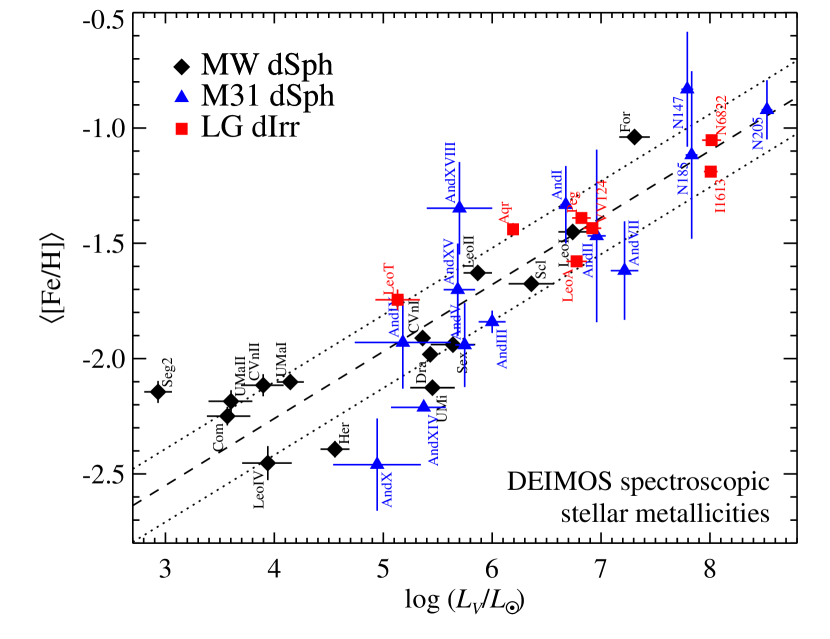
Figure 8.— The luminosity–stellar metallicity relation for Local Group dwarf galaxies. The black diamonds (MW dSphs) and red squares (dIrrs) are the average stellar iron abundances from spectroscopy of individual stars. The blue triangles (M31 dSphs) are the average stellar iron abundances from coadded spectroscopy of groups of similar stars within each dwarf galaxy. The dashed line shows the least-squares line (Equation 3, where the intercept is calculated at $10^{6}~{}L_{\sun}$), excluding the M31 data points and Segue 2, which may be a heavily tidally stripped galaxy (Kirby et al., 2013). The dotted line shows the rms about the best fit. Unlike Figure 1, there are no photometric metallicities in this figure. Hence, these data are not subject to the age–metallicity degeneracy.

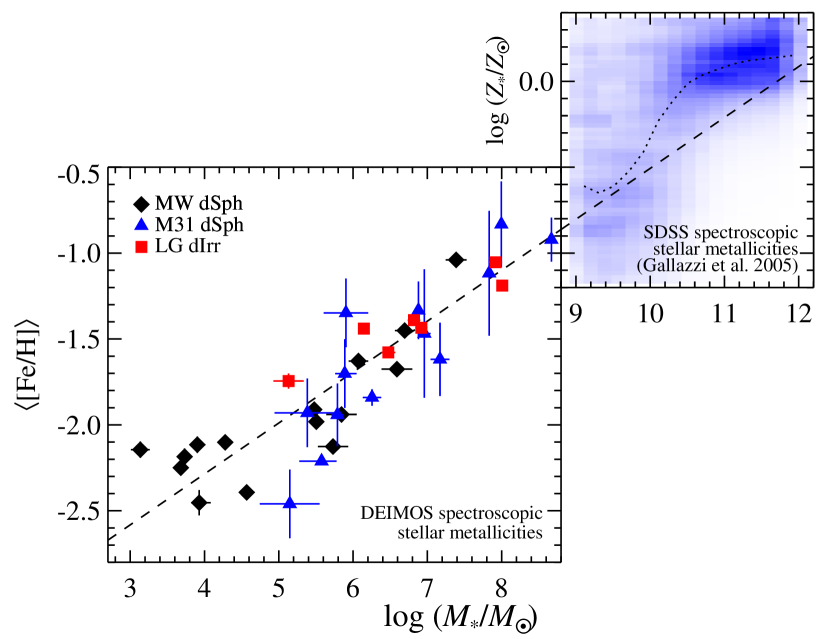
Figure 9.— The stellar mass–stellar metallicity relation for Local Group dwarf galaxies (left) and more massive SDSS galaxies galaxies (right, Gallazzi et al., 2005). The Local Group metallicities ($\langle{\rm[Fe/H]}\rangle$) were measured from iron lines, and the SDSS metallicities ($\log Z_{*}$) were measured from a combination of absorption lines, mostly Mg and Fe. The conversion between $\langle{\rm[Fe/H]}\rangle$ and $\log Z_{*}$ depends on [Mg/Fe]. The Local Group data is the same as in Figure 8, but it is plotted here versus stellar mass rather than luminosity. The dashed line is the least-squares fit to the Local Group galaxies (Equation 4, where the intercept is calculated at $10^{6}~{}M_{\sun}$), and the dotted line in the right panel is the moving median for the SDSS galaxies. Although the techniques at measuring both mass and metallicity differ between the two studies, the mass–metallicity relation is roughly continuous over nine orders of magnitude in stellar mass.

The simplest diagnostic of differential chemical evolution among galaxies is the LZR or MZR. As discussed in Section 1, Grebel et al. (2003) presented evidence that the LZR for dwarf galaxies is dichotomous between dIrrs and dSphs (see Figure 1). However, all of their MW dSph metallicities were based on spectroscopy whereas all of their dIrr metallicities were based on broadband color. Photometric metallicities are subject to the age–metallicity degeneracy, which is difficult to resolve without photometry reaching the main sequence turn-off. Only recently has such photometry become available for the dIrrs. As Lee et al. (2008) pointed out, the dichotomy in the LZR may be a result of the inability to resolve the photometric age–metallicity degeneracy for dIrrs. Lianou et al. (2011) estimated that the effect of even a small (15%) intermediate-age population is a depression of ${\rm[Fe/H]}_{\rm phot}$ by a few tenths of a dex.

In order to address the dichotomy, we calculated average metallicities from spectroscopy, which is not subject to the age–metallicity degeneracy. For each galaxy in Table 2.1, we computed a weighted mean of [Fe/H]. The metallicity of each star in the average was weighted by the inverse square of the error in [Fe/H]. For the coadded spectra of M31 satellites, the average was computed from bins of stars rather than individual stars. For those galaxies with only one bin (And IX, X, XV, and XVIII), the number presented as $\langle{\rm[Fe/H]}\rangle$ is simply the metallicity of the bin. Table 4 and Figure 8 show the resulting LZR, separated by galaxy type (dSph or dIrr).

The LZR for dSphs and dIrrs is nearly identical. The least-squares fit for the MW dSphs, accounting for measurement uncertainty in both $L_{V}$ and $\langle{\rm[Fe/H]}\rangle$ (Akritas & Bershady, 1996), is

$$\langle{\rm[Fe/H]}\rangle_{\rm dSph}=\left(-1.69\pm 0.06\right)+\left(0.29\pm 0.04\right)\log\left(\frac{L_{V}}{10^{6}~{}L_{\sun}}\right)\>.$$ (1)

We excluded Segue 2 from this fit because it may be heavily tidally stripped (Kirby et al., 2013), and its present luminosity may not reflect its luminosity when it finished forming stars. We also excluded the M31 satellites because the technique used to measure their metallicities is different and because their error bars are larger. Including them changes the slope and intercept by less than the uncertainties quoted in Equation 1. The rms of the MW dSphs about Equation 1 is $0.17$.

The LZR for the dIrrs is

$$\langle{\rm[Fe/H]}\rangle_{\rm dIrr}=\left(-1.58\pm 0.04\right)+\left(0.21\pm 0.02\right)\log\left(\frac{L_{V}}{10^{6}~{}L_{\sun}}\right)\>.$$ (2)

The rms of the dIrrs about Equation 2 is $0.09$. The rms of the dIrrs about Equation 1 is $0.12$. The dIrrs have a smaller scatter than dSphs about the best-fit line for dSphs.

We conclude that dIrrs are not deviant from the LZR defined by MW dSphs. Both types of galaxies obey the same relation. The least-squares fit for the dIrrs and MW dSphs, again excluding Segue 2, is

$$\langle{\rm[Fe/H]}\rangle=\left(-1.68\pm 0.03\right)+\left(0.29\pm 0.02\right)\log\left(\frac{L_{V}}{10^{6}~{}L_{\sun}}\right)\>.$$ (3)

The rms about the best-fit line is $0.16$. Equation 3 is the dashed line in Figure 8.

Luminosity is a direct observable, but stellar mass is more closely related to chemical evolution. The mass-to-light ratio depends on the SFH. Woo et al. (2008) calculated $M_{*}/L_{V}$ for the brighter MW dSphs and the LG dIrrs in two ways. They used modeled SFHs (Mateo, 1998), or they converted integrated galaxy colors into mass-to-light ratios based on stellar population models (Bell & de Jong, 2001; Bell et al., 2003). Generally, they preferred the SFH-based masses, but sometimes only integrated colors were available. For the fainter MW dSphs, we adopted Martin et al.’s (2008) stellar masses, which were based on modeling the distribution of stars in the CMD for each galaxy. Table 4 includes the stellar masses we adopted. For those galaxies where stellar mass measurements were not available from the aforementioned references, we assumed Woo et al.’s median SFH-based mass-to-light ratio for the appropriate galaxy type. The footnotes in Table 4 identify these galaxies.

In analogy to Figure 8 for the LZR, Figure 9 shows the MZR for the same dwarf galaxies. The least-squares fit excluding Segue 2 and the M31 satellites is

$$\langle{\rm[Fe/H]}\rangle=\left(-1.69\pm 0.04\right)+\left(0.30\pm 0.02\right)\log\left(\frac{M_{*}}{10^{6}~{}M_{\sun}}\right)\>.$$ (4)

The rms about the best-fit line is $0.17$. The scatter about the MZR is about as small as the scatter about the LZR. The similarity is expected because the variance in $M_{*}/L_{V}$ is small—especially in logarithmic space—for the predominantly old dwarf galaxies in the LG.

Ignoring possibly tidally stripped galaxies like Segue 2, the MZR is unbroken and of constant slope from the galaxies with the lowest known stellar masses up to $M_{*}=5\times 10^{8}~{}M_{\sun}$ (NGC 205), which is the upper stellar mass limit of our sample. The continuity of the relation begs the question, to what mass does the MZR persist?

The gas-phase MZR has been analyzed for many different galaxy masses, SFRs, and redshifts. Section 1 provides some background on some of those studies. However, the gas-phase metallicity depends on the instantaneous SFR or gas fraction of the galaxy (Mannucci et al., 2010; Bothwell et al., 2013). A more stable metallicity indicator is the average metallicity, $\langle{\rm[Fe/H]}\rangle$, of the stars. Besides, our measurements are of stellar metallicities. After all, the dSphs have no gas for which we could measure metallicity. Therefore, it makes sense to compare our dwarf galaxy MZR to a study of more massive galaxies with measurements of stellar metallicity.

Gallazzi et al. (2005, 2006) compiled the largest sample of galactic stellar metallicities. They measured ages, metallicities, and an empirical proxy for [$\alpha$/Fe] ratios for tens of thousands of SDSS galaxies. The right panel of Figure 9 shows a Hess diagram of their MZR. Although both our measurements and those of Gallazzi et al. are stellar metallicities, they were not measured in the same manner. We measured [Fe/H] from iron absorption lines in individual stars. Gallazzi et al. measured metallicities using broad spectral features, dominated by Mg and Fe, in the integrated light of galaxies. The $y$-axis labels in Figure 9 discriminate between the pure iron abundances and SDSS “metallicities” by calling them $\langle{\rm[Fe/H]}\rangle$ and $\log(Z_{*}/Z_{\sun})$, respectively. The conversion from $\langle{\rm[Fe/H]}\rangle$ to $\log Z_{*}$ depends on [Mg/Fe]. For solar abundance ratios, $\langle{\rm[Fe/H]}\rangle$ and $\log Z_{*}$ are directly comparable. The measurements also differ in many other ways, such as the method of taking the average (averaging individual stars versus light-weighted mean), the stellar population probed (red giants versus the entire stellar population), and the models used (Kirby et al. 2010 versus Bruzual & Charlot 2003).

Despite the different techniques in measuring average metallicity and stellar mass, these two samples are the best available to merge together to form one MZR from the lowest to highest galaxy masses. The dashed line in Figure 9 is the best fit to the LG dwarf galaxies (Equation 4). The dotted line in the right panel shows the moving median of the SDSS galaxies. The shape of the MZR for dwarf galaxies is a straight line in log–log space, but the shape for the more massive galaxies flattens at higher metallicity. The flattening also happens in the gas-phase MZR (Tremonti et al., 2004; Andrews & Martini, 2013; Zahid et al., 2013). At least some of this flattening is due to aperture bias of the SDSS fibers (also see Kauffmann et al., 2003). The more massive galaxies are rare and preferentially farther away. The fixed angular size of the fiber covers a larger fraction of these more massive, more distant galaxies. Radial metallicity gradients cause a larger fraction of the outermost, metal-poor stars to be included in the more massive galaxies. In any case, the MZRs for the dwarf galaxies and the SDSS galaxies are roughly continuous across the boundary between the two samples of galaxies at $M_{*}=10^{9}~{}M_{\sun}$. The MZR slope is not quite the same at the $M_{*}$ boundary, but again, the techniques at measuring stellar metallicities in the two samples are not homogeneous.

A possible origin of the MZR is metal loss. Galaxies with deeper gravitational potential wells are able to retain supernova ejecta more readily than less massive galaxies (e.g., Dekel & Silk, 1986). The less massive galaxies lose gas and metals to supernova winds, and their stars end up more metal-poor.

The success of feedback in explaining the MZR implies that dwarf galaxies are extremely susceptible to metal loss. Kirby et al. (2011b) showed that the MW satellite galaxies lost more than 96% of the iron that their stars produced. That conclusion was based simply on the stellar masses of the galaxies, theoretical nucleosynthetic yields, and present stellar metallicities. This metal loss could have been caused by any gas loss mechanism, including supernova feedback (e.g., Murray et al., 2005), radiation pressure (e.g., Murray et al., 2011), tidal stripping, or ram pressure stripping (e.g., Mayer et al., 2001).

The dIrr galaxies fall on the same MZR. The same argument about metal loss can be applied to them with one modification. The MW dSphs have no gas today, but dIrrs do have gas. This difference alone implicates gas stripping as a major cause for gas and metal removal from the dSphs (e.g., Lin & Faber, 1983). Any metals not present in dIrrs’ stars could be present in the gas. Gavilán et al. (2013) proposed that dIrrs could indeed evolve with no metal loss. Instead, gas infall combined with low star formation efficiencies (high gas mass fractions) can be responsible for the low metallicities of dIrrs (also see Matteucci 1994 and Calura et al. 2009). This scenario would lead to high gas-phase metallicities.

However, the gas-phase metallicities of dIrrs are not especially high. As an example, based on supernova yields (Iwamoto et al., 1999; Nomoto et al., 2006) and a Type Ia supernova delay time distribution (Maoz et al., 2010), the stellar population in NGC 6822 should have produced $3\times 10^{5}~{}M_{\sun}$ of iron. Based on their average metallicity ($\langle{\rm[Fe/H]}\rangle=-1.05$), the stars in NGC 6822 harbor just 5% of this iron. If the remaining iron were in the gas ($M_{\rm HI}=1.3\times 10^{8}~{}M_{\sun}$, Koribalski et al., 2004), then the metallicity of the gas would be ${\rm[Fe/H]}=+0.1$. The gas-phase oxygen abundance is ${\rm[O/H]}=-0.55\pm 0.10$ (Lee et al., 2006b). Therefore, the gas would have ${\rm[O/Fe]}=-0.7$ if the galaxy never lost its iron. This value is at odds with the stellar ratio (${\rm[O/Fe]}=+0.1$, Venn et al., 2001) measured from young A supergiants. Furthermore, the MZR shows no trend with gas fraction. DIrrs with gas-to-stellar mass ratios less than one, like IC 1613 and VV 124, do not show any deviation from the MZR compared to gas-rich dIrrs. We conclude that the missing iron is no longer part of stars or the star-forming gas. Our present measurements do not inform us whether the missing iron has left the galaxy or has been incorporated into a hot gas halo (Shen et al., 2012, 2013).

We have established that a single MZR applies to all LG galaxies with $10^{3.5}<M_{*}/M_{\sun}<10^{9}$, but we have not shown that all galaxies in the universe obey such a tight relation. Gallazzi et al. (2005, 2006) separated more massive galaxies in the MZR into high and low concentration groups. The high-concentration galaxies have lower SFRs than the low-concentration galaxies. The two groups also follow different MZRs. The high-concentration galaxies have higher metallicities on average, especially in the mass range $10^{9}<M_{*}/M_{\sun}<10^{10.5}$. The low-concentration galaxies have a larger scatter in metallicity at fixed stellar mass. The model of Magrini et al. (2012) explains these trends in the context of star formation efficiency without invoking mass loss. Denser galaxies (presumably with denser gas) form stars more efficiently and end up with higher metallicities. Furthermore, satellite galaxies appear to be more metal-rich at fixed halo or stellar mass than central galaxies (Pasquali et al., 2010). Therefore, there is a parameter other than $M_{*}$ that controls the slope, offset, and scatter of the MZR for more massive galaxies.

Our findings also cannot explain the offset in the MZR between dSphs and dIrrs from abundances of PNe (Richer et al., 1998; Gonçalves et al., 2007). PNe in dSphs are found to have very high oxygen abundances compared to their stellar iron metallicities. For example, the field population of Fornax hosts one PN, which has an oxygen abundance between ${\rm[O/H]}=-0.7$ and $-0.3$ (Maran et al., 1984; Richer & McCall, 1995; Kniazev et al., 2007). For comparison, the stellar iron abundance is $\langle{\rm[Fe/H]}\rangle=-1.04$. NGC 205 is another dSph/dE with very oxygen-rich PNe. Richer & McCall (1995) reported its mean PN abundance at ${\rm[O/H]}=-0.1$. We measured its mean stellar iron abundance as $\langle{\rm[Fe/H]}\rangle=-0.92$. Similarly, the PN abundances for NGC 147 and 185 are ${\rm[O/H]}=-0.6$ (Gonçalves et al., 2007) and $-0.5$ (Richer & McCall, 1995), respectively, whereas our stellar metallicities are $\langle{\rm[Fe/H]}\rangle=-0.83$ and $-1.12$. It is possible that the PN abundances are overestimated. For example, Richer & McCall’s average PN abundances were based on lower limits on the abundances for several PNe in each galaxy. As an example, the lower limits on individual PNe in NGC 205 are up to 27 times smaller than the quoted mean for the galaxy. Perhaps the method of averaging lower limits leads to a bias in the quoted abundance. Alternatively, the dSph PNe themselves might produce oxygen in the third dredge-up (Magrini et al., 2005; Kniazev et al., 2007). The PNe might also be sampling a younger population of stars that are preferentially more metal-rich than the population average. In the future, we will use measurements of stellar magnesium abundances to compare to the oxygen abundances in the PNe because oxygen is nucleosynthetically much more closely related to magnesium than iron.

5. Galactic Chemical Evolution

Table 5Chemical Evolution Models

	Leaky Box		Pre-Enriched				Accretion
dSph	$p_{\rm eff}$ ($Z_{\sun}$)		$p_{\rm eff}$ ($Z_{\sun}$)	${\rm[Fe/H]}_{0}$	$\Delta{\rm AICc}$		$p_{\rm eff}$ ($Z_{\sun}$)	$M$	$\Delta{\rm AICc}$	Best Model
MW dSphs
Fornax	$0.106\pm 0.005$		$0.082_{-0.004}^{+0.005}$	$-2.05\pm 0.06$	+$124.03$		$0.111\pm 0.003$	$9.3_{-1.3}^{+1.5}$	$306.90$	Accretion
Leo I	$0.041\pm 0.002$		$0.030\pm 0.002$	$-2.33_{-0.06}^{+0.05}$	+$178.41$		$0.043\pm 0.001$	$7.9_{-1.0}^{+1.2}$	$353.33$	Accretion
Sculptor	$0.029\pm 0.002$		$0.027\pm 0.002$	$-3.39_{-0.26}^{+0.18}$	+0$10.72$		$0.029\pm 0.002$	$1.4\pm 0.2$	00$5.32$	Pre-Enriched
Leo II	$0.028\pm 0.002$		$0.024\pm 0.002$	$-2.92_{-0.13}^{+0.11}$	+0$25.47$		$0.028\pm 0.002$	$3.3_{-0.5}^{+0.7}$	0$45.22$	Accretion
Sextans	$0.016\pm 0.002$		$0.013\pm 0.002$	$-3.17_{-0.23}^{+0.16}$	+0$12.01$		$0.014\pm 0.001$	$3.3_{-1.0}^{+1.8}$	0$10.43$	Pre-Enriched
Ursa Minor	$0.011\pm 0.001$		$0.007\pm 0.001$	$-2.92_{-0.10}^{+0.09}$	+0$41.85$		$0.009\pm 0.001$	$11.0_{-4.5}^{+5.6}$	0$44.30$	Accretion
Draco	$0.014\pm 0.001$		$0.011\pm 0.001$	$-3.06_{-0.10}^{+0.09}$	+0$37.67$		$0.013\pm 0.001$	$4.2_{-0.9}^{+1.3}$	0$44.70$	Accretion
Can. Ven. I	$0.019\pm 0.002$		$0.016\pm 0.002$	$-3.10_{-0.20}^{+0.15}$	+0$13.39$		$0.017_{-0.001}^{+0.002}$	$2.6_{-0.7}^{+1.0}$	00$9.62$	Pre-Enriched
Local Group dIrrs
NGC 6822	$0.129\pm 0.008$		$0.127_{-0.008}^{+0.009}$	$<-2.93$	00$-1.92$		$0.126_{-0.007}^{+0.008}$	$1.7_{-0.2}^{+0.3}$	00$6.95$	Accretion
IC 1613	$0.078_{-0.007}^{+0.008}$		$0.058_{-0.006}^{+0.007}$	$-2.08_{-0.11}^{+0.09}$	+0$29.82$		$0.075_{-0.005}^{+0.006}$	$4.3_{-1.1}^{+1.5}$	0$22.73$	Pre-Enriched
VV 124	$0.043_{-0.006}^{+0.007}$		$0.042_{-0.006}^{+0.007}$	$<-3.37$	00$-2.12$		$0.041\pm 0.006$	$1.5_{-0.3}^{+0.7}$	0$-2.63$	Leaky Box
Peg. dIrr	$0.058_{-0.006}^{+0.007}$		$0.058_{-0.006}^{+0.007}$	$<-3.87$	00$-2.09$		$0.058\pm 0.006$	$1.4_{-0.2}^{+0.4}$	0$-1.76$	Leaky Box
Leo A	$0.033\pm 0.006$		$0.030_{-0.006}^{+0.007}$	$-3.06_{-2.88}^{+0.44}$	+00$2.17$		$0.030\pm 0.004$	$6.2_{-3.0}^{+4.1}$	00$2.13$	Pre-Enriched
Aquarius	$0.044_{-0.009}^{+0.012}$		$0.039_{-0.010}^{+0.012}$	$<-2.08$	00$-0.11$		$0.040_{-0.006}^{+0.007}$	$5.6_{-2.7}^{+3.7}$	00$2.87$	Accretion
Leo T	$0.021_{-0.006}^{+0.008}$		$0.021_{-0.006}^{+0.007}$	$<-4.93$	00$-2.49$		$0.020\pm 0.005$	$4.1_{-2.1}^{+6.3}$	0$-2.12$	Leaky Box

Note. — Error bars represent 68% confidence intervals. Upper limits are at 95% (2$\sigma$) confidence.

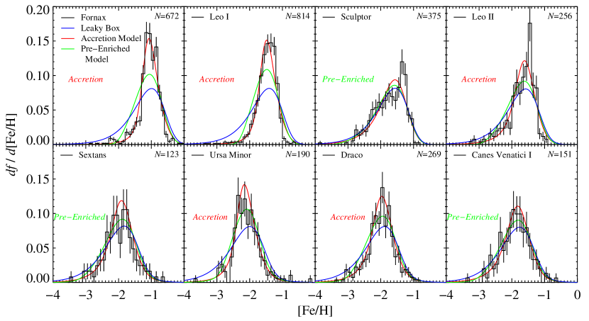
Figure 10.— The metallicity distributions for the eight most luminous MW dSphs in our sample. The galaxies are arranged from most luminous (Fornax) to least luminous (Canes Venatici I). The colored lines show the maximum likelihood fits of three different chemical evolution models convolved with the measurement uncertainties. The colored, italicized text indicates the preferred model.

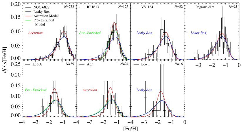
Figure 11.— The metallicity distributions for the dIrrs in our sample. The galaxies are arranged from most luminous (NGC 6822) to least luminous (Leo T). Whereas the Accretion Model is generally a better description of dSphs (Figure 10), the Leaky Box or Pre-Enriched Models are fair descriptions of the dIrrs.

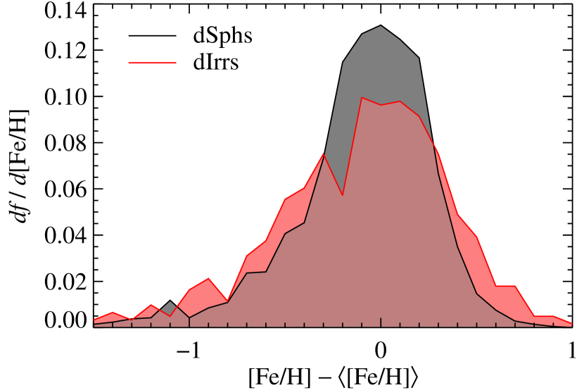
Figure 12.— The combined MDFs for the luminous dSphs in Figure 10 (black) and the luminous dIrrs in Figure 11 (red). Only galaxies with $M_{*}>10^{6}~{}M_{\sun}$ were included in the stacked MDFs. Each individual galaxy’s MDF was centered at its mean [Fe/H] before the MDFs were stacked together. The average MDF for dIrrs is broader and less peaked than the average MDF for dSphs.

Because we measured metallicities of individual stars in the dIrrs and MW dSphs, we can analyze the metallicity distribution function (MDF) rather than just the mean metallicity. The MDF encodes the star formation and gas flow history of the galaxy. The shape of the MDF indicates whether the galaxy conforms to a closed box or whether it accreted gas during its star formation lifetime. Figure 10 shows the MDFs for the MW dSphs. This figure is nearly the same as Figure 1 of Kirby et al. (2011a). We show it here to contrast the dSphs with the dIrrs, whose MDFs are shown in Figure 11. Only stars with measurement uncertainties $\delta{\rm[Fe/H]}<0.5$ are included in those figures and in the following discussion.

The MDFs of the dIrrs are shaped differently from the dSphs, even at the same luminosity or stellar mass. Three of the most luminous MW dSphs—Fornax, Leo I, and Leo II—have narrowly peaked distributions with a metal-poor tail. Sculptor and the four least luminous MW dSphs in Figure 10 have broader MDFs. The dIrr MDFs are also broader even though six of the seven dIrrs have luminosities similar to Leo I and Fornax. Figure 12 illustrates the different shapes. The average MDF for the dIrrs with $M_{*}>10^{6}~{}M_{\sun}$ is broader and less peaked than the average MDF for dSphs in the same stellar mass range. The two-sided Kolmogorov–Smirnov test gives a probability of $0.02\%$ that the distributions in Figure 12 are drawn from the same parent distribution.

Some of the difference in MDF shape between dSphs and dIrrs may reflect the different SFHs between the two types of galaxies. Because dIrrs generally have more extended SFHs than dSphs (Mateo, 1998; Orban et al., 2008), they could have different [$\alpha$/Fe] ratios. The dSph and dIrr MDFs of an $\alpha$ element, like oxygen or magnesium, might be less diverse than the MDFs of iron. Our spectral synthesis technique of measuring abundances is sensitive to some $\alpha$ elements. In a future article, we will compare MDF shapes of elements other than iron.

The uniformity of the MZR is even more remarkable in light of the differently shaped MDFs. Somehow, the mean metallicity of a dwarf galaxy depends only on its stellar mass, regardless of how the metallicities of individual stars are distributed about the mean. We return to this discussion in Section 5.1.

The shape of a galaxy’s MDF can be understood in the context of its history of star formation and gas flow. For example, the accretion of external, metal-poor gas can lower the metallicity of the galaxy’s star-forming interstellar medium (ISM). However, the presence of new gas also triggers star formation, which raises the ISM metallicity. These effects can counteract each other to keep the ISM metallicity roughly constant while stars are forming. Therefore, accretion of external gas can cause a peak in the MDF around a single metallicity.

5.1. Chemical Evolution Models

Quantitative models of galactic chemical evolution can be used to interpret the shape of the MDF. Kirby et al. (2011a) fit three different models of chemical evolution to the eight dSphs in Figure 10. We re-fit the same models to the dSph MDFs, updated as described in Section 3.2. We also fit the same models to the dIrrs.

All of the following analytic models assume the instantaneous mixing and instantaneous recycling approximations. The latter approximation is not particularly appropriate for elements that have production timescales delayed with respect to star formation. For example, iron is produced mostly in Type Ia SNe, which are delayed with respect to star formation. It would be more appropriate to compare our models to oxygen abundance distributions because oxygen production closely tracks star formation. However, iron is the best measured stellar metallicity indicator available to us. It must be kept in mind that the instantaneous recycling approximation is a weakness in the following models.

The simplest model is the Leaky Box (called the Pristine Model by Kirby et al., 2011a). In this model, the galaxy begins its life with all the gas it will ever have. The gas is initially metal-free. It may turn into stars or be expelled from the galaxy. The galaxy is not allowed to accrete new gas. The functional form of the Leaky Box is the same as the Closed Box (Schmidt, 1963; Talbot & Arnett, 1971; Searle & Sargent, 1972). The only difference is that the stellar nucleosynthetic yield ($p$) in the Closed Box becomes the effective yield ($p_{\rm eff}$) in the Leaky Box. The definition of effective yield subsumes metal loss from the galaxy. The effective yield is the yield of metals that participate in forming the next generation of stars. The MDF of the Leaky Box is

$$\frac{dN}{d{\rm[Fe/H]}}\propto\left(\frac{10^{{\rm[Fe/H]}}}{p_{\rm eff}}\right)\exp\left(-\frac{10^{{\rm[Fe/H]}}}{p_{\rm eff}}\right)\>.$$ (5)

The only free parameter is $p_{\rm eff}$.

The Pre-Enriched Model (Pagel, 1997) is a generalization of the Leaky Box, but the initial gas has a metallicity ${\rm[Fe/H]}_{0}$. The MDF of the Pre-Enriched Model is

$$\frac{dN}{d{\rm[Fe/H]}}\propto\left(\frac{10^{{\rm[Fe/H]}}-10^{{\rm[Fe/H]}_{0}}}{p_{\rm eff}}\right)\exp\left(-\frac{10^{{\rm[Fe/H]}}}{p_{\rm eff}}\right)\>.$$ (6)

The two free parameters are $p_{\rm eff}$ and ${\rm[Fe/H]}_{0}$.

The Accretion model (called the Extra Gas Model by Kirby et al., 2011a) is also a generalization of the Leaky Box. Lynden-Bell (1975) invented this model and called it the Best Accretion Model. The initial metallicity is zero, but gas is allowed to flow into the galaxy according to a specific functional form. The MDF is described by two transcendental equations that must be solved for the stellar mass fraction, $s$.

$${\rm[Fe/H]}(s) = \log\bigg{\{}p_{\rm eff}\left(\frac{M}{1+s-\frac{s}{M}}\right)^{2}\times$$ (7)

$$\left[\ln\frac{1}{1-\frac{s}{M}}-\frac{s}{M}\left(1-\frac{1}{M}\right)\right]\bigg{\}}$$

$$\frac{dN}{d{\rm[Fe/H]}} \propto \frac{10^{{\rm[Fe/H]}}}{p_{\rm eff}}\times$$ (8)

$$\frac{1+s\left(1-\frac{1}{M}\right)}{\left(1-\frac{s}{M}\right)^{-1}-2\left(1-\frac{1}{M}\right)\times 10^{{\rm[Fe/H]}}/p_{\rm eff}}$$

The two free parameters are $p_{\rm eff}$ and the accretion parameter, $M$, which is the ratio of the final mass to the initial gas mass.

We found the most likely parameters for all three models for all of the dSphs in Figure 10 and dIrrs in Figure 11. Following the same procedure as Kirby et al. (2011a), we maximized the likelihood that the model described the observed MDF with a Monte Carlo Markov chain. The length of the chain was $10^{3}$ trials for the Leaky Box and $10^{5}$ trials for the Pre-Enriched and Accretion Models. Table 5 gives those parameters along with the 68% likelihood intervals. Figures 10 and 11 show the best-fitting model MDFs convolved with functions that approximate the observational uncertainties for each galaxy. Thus, the model curves in Figure 11 already reflect that the measurement uncertainties are larger on average for the dIrrs compared to the dSphs.

The Pre-Enriched and Accretion Models are generalizations of the Leaky Box. They always fit the MDF better than the Leaky Box because they have two free parameters rather than one. However, introducing a free parameter into a model risks over-fitting the data. The Bayesian information criterion is a statistic that estimates whether the extra free parameter is necessary. A revision to this statistic is the Akaike information criterion (AIC, Akaike, 1974). Sugiura (1978) revised this statistic and called it the corrected AIC (AICc):

$${\rm AICc}=-2\ln L+2r+\frac{2r(r+1)}{N-r-1}$$ (9)

where $L$ is the maximum likelihood of the model, $r$ is the number of free parameters, and $N$ is the number of stars. Table 5 includes the value $\Delta{\rm AICc}$, which is the difference between the AICc of the Pre-Enriched or Accretion Model and the Leaky Box. Positive values of $\Delta{\rm AICc}$ indicate that the introduction of the extra free parameter is justified and that the more complicated model fits better. Negative values of $\Delta{\rm AICc}$ indicate that the extra free parameter is an unnecessary complication. The best model—the one with the largest AICc—is indicated in Table 5 and in colored text in Figures 10 and 11.

The Leaky Box is not the best model to describe any of the dSphs. Five of the dSphs require the accretion of pristine gas to explain the shapes of their MDFs. Three of the dSphs are better described by the Pre-Enriched Model.

On the other hand, the Leaky Box is the best model to describe the MDFs of three of seven dIrrs. The Accretion Model is the best model only for NGC 6822 and Aquarius. Even in those two cases, $\Delta{\rm AICc}$ is over six times smaller than $\Delta{\rm AICc}$ for any of the dSph MDFs that prefer the Accretion Model. In other words, those two dIrrs prefer the Accretion Model, but not nearly as much as the dSphs.

Again, the uniformity of the MZR is remarkable in light of the different gas flow histories implied by the MDF shapes. Despite the varying importance of gas accretion and pre-enrichment, the mean metallicity of dwarf galaxies is strictly a function of stellar mass. The metallicity of any Closed Box galaxy approaches the nucleosynthetic yield, regardless of stellar mass. The average metallicity of a Leaky Box is lower than the true yield only by virtue of the expulsion of metals from the galaxy. Therefore, the MZR can be interpreted as a relation between stellar mass and metal loss.

However, the variable that controls metal loss is more likely to be the depth of the gravitational potential well than stellar mass. Therefore, the MZR may indicate that the stellar mass is an excellent tracer of potential well depth. Massive galaxies with deeper wells retain more gas and hence form more stars. Retention of gas goes hand in hand with retention of metals produced by the stellar population. The details of how the galaxy acquired the gas are not important.

In support of this interpretation of the MZR, Gallazzi et al. (2006) showed that the average stellar metallicity of SDSS galaxies is a tighter function of dynamical mass (essentially velocity dispersion) than stellar mass (although we note that Tollerud et al. 2011 found that finding the total, virial masses is not straightforward even for massive elliptical galaxies). Unfortunately, the velocity dispersion of dwarf galaxies traces only the innermost mass. The half-light radius is much smaller than the half-mass radius for galaxies with $\sigma_{v}\lesssim 10$ km s^-1 (see, e.g., Wolf et al., 2010). Consequently, the dynamical masses of the dwarf galaxies in our sample are virtually unconstrained compared to the SDSS galaxies. We cannot directly test the hypothesis that the fundamental independent variable of the MZR is potential well depth (virial mass) rather than stellar mass without assuming a strong theoretical relation between inner mass and virial mass.

5.2. Ram Pressure Stripping

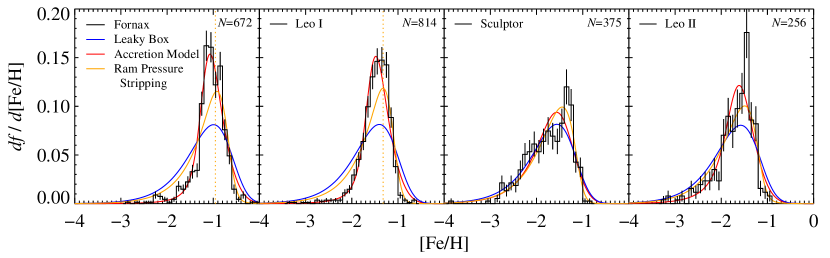
Figure 13.— The metallicity distributions for the four most luminous dSphs in our sample. This figure is the same as the top row of Figure 10 except that the Ram Pressure Stripping Model replaces Pre-Enriched Model. The dotted orange line indicates ${\rm[Fe/H]}_{s}$, the metallicity at which ram pressure stripping turns on, in the two cases where it was able to be constrained.

Table 6Ram Pressure Stripping Model of Chemical Evolution

	Ram Pressure Stripping
dSph	$p_{\rm eff}$ ($Z_{\sun}$)	${\rm[Fe/H]}_{s}$	$\zeta$	$\Delta{\rm AICc}$
Fornax	$0.465_{-0.101}^{+0.082}$	$-0.95\pm 0.05$	$2.01_{-0.70}^{+0.61}$	+$177.74$
Leo I	$0.178_{-0.033}^{+0.022}$	$-1.32_{-0.05}^{+0.04}$	$2.30_{-0.65}^{+0.23}$	+$242.12$
Sculptor	$0.079_{-0.019}^{+0.048}$	$<-1.41$	$0.43_{-0.17}^{+0.53}$	+0$21.88$
Leo II	$0.165_{-0.061}^{+0.027}$	$<-3.74$	$1.68_{-0.82}^{+0.31}$	+0$43.26$

None of the models is a great fit to the MDFs of the four most luminous MW dSphs in our sample (Fornax, Leo I, Sculptor, and Leo II). The observed MDFs approach a wall in [Fe/H] at the metal-rich end. None of the three models we presented so far can explain the sharpness of the wall. All three models overpredict the number of the most metal-rich stars. None of the dIrrs or the four least luminous dSphs show this feature.

As the MW’s satellite galaxies orbit around it, they pass through the hot gas corona. This corona can exert ram pressure on the galaxy’s gas. Hydrodynamical models (e.g., Mayer et al., 2006) show that ram pressure stripping is effective at removing all of the gas from a galaxy after just a couple pericentric passages. In a new model (Gatto et al., 2013) that incorporates supernova feedback, the MW removes all of the gas from an infalling satellite galaxy in just one pericentric passage. The timescale for gas removal can be as short as 0.5 Gyr.

The LG galaxies show evidence for ram pressure stripping. Grcevich & Putman (2009) showed that nearly all galaxies within 270 kpc of the MW or M31 have no gas. Nearly all galaxies outside that boundary do have gas. Proximity to a large host galaxy is very effective at removing gas. Grcevich & Putman argued that the most likely culprit is ram pressure stripping.

Rapid, efficient removal of gas can explain the sharp, metal-rich cut-offs we observed for Fornax, Leo I, Sculptor, and Leo II. A simple modification to the Leaky Box model can predict the shape of the metallicity distribution in the presence of ram pressure stripping. This model is similar to the “constant velocity flow” model of Edmunds & Greenhow (1995). We assume that gas is removed at a constant rate starting at time $t_{s}$. Because the model has just one zone, time $t_{s}$ corresponds to a metallicity $Z_{s}$.

At time $t=0$, the galaxy consists only of gas, and the gas mass fraction is $g=1$. The stellar mass fraction is $s$. In the absence of inflowing gas, the gas fraction is depleted by the outflow rate ($E$) and the SFR.

$$\frac{dg}{dt} = -E-\frac{ds}{dt}$$ (10)

$$\frac{dg}{ds} = -\frac{E+ds/dt}{ds/dt}$$ (11)

Pagel (1997) derived the following relation between $g$, $s$, metallicity ($Z$), and the nucleosynthetic yield ($p$) in the absence of accretion.

$$g\frac{dZ}{ds}=p$$ (12)

For convenience, we define $z\equiv Z/p$ such that $g\;dz/ds=1$. Combining Equations 11 and 12,

$$g\frac{dz}{dg}=-\frac{ds/dt}{E+ds/dt}\>.$$ (13)

For simplicity, we assume that the SFR is proportional to the gas mass.

$$ds/dt=\beta g$$ (14)

This is a simplified version of the Kennicutt–Schmidt law.

Now we assume that the gas outflow rate has a term proportional to the SFR, such as would be the case with supernova feedback, and a constant term that turns on after a time $t_{s}$, which mimics the commencement of ram pressure stripping.

$$E = \eta\frac{ds}{dt}+E_{s}^{\prime}$$ (15)

$$E_{s}^{\prime} = \left\{\begin{array}[]{ll}0&\mbox{ if $t<t_{s}$ or $z<z_{s}$}\\ E_{s}&\mbox{ if $t\geq t_{s}$ or $z\geq z_{s}$}\end{array}\right.$$ (18)

Equation 13 becomes

$$g\frac{dz}{dg} = -\frac{\beta g}{(1+\eta)\beta g+E_{s}^{\prime}}\>.$$ (19)

$$dz = -\frac{\beta\;dg}{(1+\eta)\beta g+E_{s}^{\prime}}$$ (20)

$$e^{-(1+\eta)z} \propto (1+\eta)\beta g+E_{s}^{\prime}$$ (21)

We require that $g=1$ at $z=0$, and we require continuity in the function $g$ at $t=t_{s}$. These conditions combined with Equation 15 and 18 yield

$$g=\left\{\begin{array}[]{ll}e^{-(1+\eta)z}&\mbox{ if $z<z_{s}$}\\ \left[1+\frac{E_{s}e^{(1+\eta)z_{s}}}{(1+\eta)\beta}\right]e^{-(1+\eta)z}-\frac{E_{s}}{(1+\eta)\beta}&\mbox{ if $z\geq z_{s}$}\end{array}\right.\>.$$ (22)

For simplicity, we define a stripping parameter $\zeta\equiv E_{s}/((1+\eta)\beta)$. As for the Leaky Box model, an effective yield can also be defined: $p_{\rm eff}\equiv p/(1+\eta)$ and $z\equiv Z/p_{\rm eff}$.

The metallicity distribution in this model can be represented as follows.

$$\frac{ds}{d\log z} = (\ln 10)z\frac{ds}{dz}$$ (23)

$$= (\ln 10)zg$$ (24)

$$= \left\{\begin{array}[]{ll}(\ln 10)ze^{-z}&\mbox{ if $z<z_{s}$}\\ (\ln 10)z\left[e^{-z}+\zeta\left(e^{z_{s}-z}-1\right)\right]&\mbox{ if $z\geq z_{s}$}\end{array}\right.$$ (27)

The first case ($z<z_{s}$) is identical to Equation 5. The second case can be rewritten as

$$\frac{dN}{d{\rm[Fe/H]}} \propto \left(\frac{10^{{\rm[Fe/H]}}}{p_{\rm eff}}\right)\Bigg{[}\exp\left(-\frac{10^{{\rm[Fe/H]}}}{p_{\rm eff}}\right)+$$ (28)

$$\zeta\left(\exp\left(\frac{10^{{\rm[Fe/H]}_{s}}-10^{{\rm[Fe/H]}}}{p_{\rm eff}}\right)-1\right)\Bigg{]}\>.$$

The three free parameters are $p_{\rm eff}$, ${\rm[Fe/H]}_{s}$, and $\zeta$.

We fit Equation 28 to the MDFs of Fornax, Leo I, Sculptor, and Leo II in the same manner that we fit the Pre-Enriched and Accretion Models. Figure 13 shows the Ram Pressure Stripping Model compared to the Leaky Box and Accretion Models. The dotted lines in the panels for Fornax and Leo I show ${\rm[Fe/H]}_{s}$. In the cases of Sculptor and Leo II, ${\rm[Fe/H]}_{s}$ is very small. In other words, ram pressure stripping turned on at the same time that the galaxy started to form its first, most metal-poor stars. Table 6 gives the best-fitting model parameters as well as $\Delta{\rm AICc}$ compared to the Leaky Box.

The Ram Pressure Stripping Model fits all four dSphs better than the Leaky Box, even after accounting for the addition of an extra two free parameters. In particular, the new model reproduces the sharpness of the metal-rich cut-off. In fact, the model was designed to do so.

However, the Ram Pressure Stripping Model is the best fit of all four models only for Sculptor. Fornax, Leo I, and Leo II prefer the Accretion Model, although the difference between the two models for Leo II is tiny. It is too simplistic to apply ram pressure stripping to a Leaky Box to explain the MDF shapes of the dSphs. It would be better to apply ram pressure stripping to the Accretion Model to explain the MDFs of Fornax and Leo I. We did not attempt to do so. Rather our modification of the Leaky Box model already illustrates the point that gas stripping can describe the metal-rich cut-offs.

The dIrrs and the four least luminous dSphs in our sample do not have sharp metal-rich cut-offs. The Ram Pressure Stripping Model is not required to explain their MDFs. It makes sense that dIrrs have not encountered ram pressure stripping. They are far from large galaxies with gas halos that could strip them. On the other hand, the low-luminosity dSphs do orbit the MW at distances small enough to encounter ram pressure stripping. The fact that their MDFs show no evidence for stripping may indicate that they finished their star formation before they fell into the MW. This interpretation is consistent with the exclusively ancient populations in Sextans (Orban et al., 2008), Ursa Minor (Mighell & Burke, 1999), Draco (Grillmair et al., 1998; Aparicio et al., 2001), and Canes Venatici I (Okamoto et al., 2012). On the other hand, Fornax (Coleman & de Jong, 2008) and Leo I (Held et al., 2001) had SFHs easily extended enough to be affected by ram pressure stripping. While ram pressure stripping likely ended star formation in Fornax and Leo I, something else ended star formation in the less luminous dSphs. Suspects are reionization—as long as it happened gradually enough to fail to produce a metal-rich cut-off in the MDF—and supernova feedback. We note that Monelli et al. (2010) and Hidalgo et al. (2011) found no evidence for the effects of reionization on the SFHs of isolated dwarf galaxies.

The differently shaped MDFs between dSphs and dIrrs pose a problem for the theory that dIrrs transform into dSphs (Lin & Faber, 1983; Mayer et al., 2001) unless tidal stripping removed many metal-poor stars from dSphs as they fell into the MW (see Section 3.4). Most of the dSphs have MDFs that seem to require gas accretion. Even incorporating an environmental effect, like ram pressure stripping, cannot avoid the fact that the MDF shapes of Fornax and Leo I are not Leaky Boxes. Sextans, Ursa Minor, Draco, and Canes Venatici I are neither Leaky Boxes nor ram pressure stripped. Their MDF shapes are not that simple. On the other hand, the dIrr MDF shapes are fairly simple. Even the dIrrs that prefer the Accretion Model have only a slight preference (comparatively small values of $\Delta{\rm AICc}$). Additionally, NGC 6822 has a low accretion parameter of $M=1.7^{+0.2}_{-0.3}$. The accretion parameters for the dSphs that prefer the Accretion Model range from $M=3.3^{+0.5}_{-0.7}$ (Leo II) to $11.0^{+4.5}_{-5.6}$ (Ursa Minor). In other words, the dSph MDFs are not consistent with transforming the dIrr MDFs via removal of gas associated with falling into the MW.

We have presented a limited set of chemical evolution models. It is possible that the Accretion Model fits the MDFs deceptively well. The physical interpretation of the model is not necessarily the truth of the galaxy’s history just because it fits the MDF. More complex models may better reflect the dSphs’ SFH. For example, Fornax experienced multiple discrete episodes of star formation rather than one smoothly varying SFR (Buonanno et al., 1999; Saviane et al., 2000; Battaglia et al., 2006; Gullieuszik et al., 2007; Coleman & de Jong, 2008). A proper chemical evolution model should incorporate multiple episodes of star formation, the accompanying expulsion of gas, and the possible subsequent re-accretion of gas (e.g., see the chemical evolution models of Romano et al. 2006 and Yin et al. 2010). It is also possible that galaxies as large as Fornax were not completely ram pressure stripped on their first pericentric approach to the MW. After all, simulations of tidal stirring (e.g., Mayer et al., 2006; Kazantzidis et al., 2011; Łokas et al., 2011) require multiple pericentric passages to complete the transformation of a dIrr into a dSph. It may be appropriate to add complexity to our Ram Pressure Stripping Model to account for multiple pericentric passages. This is best achieved in hydrodynamical simulations (e.g., Mayer et al., 2006; Gatto et al., 2013).

6. Summary and Conclusions

We measured metallicities from spectra of individual red giants in 15 MW dSphs and seven LG dIrrs as well as from coadded spectra of red giants in 13 M31 dSphs. In contrast to metallicities measured from emission lines, our stellar metallicities were not affected by the instantaneous gas fraction in the galaxies. Instead, they are a chronicle of the galaxies’ past star formation. Unlike integrated light spectroscopy, resolving individual stars also allowed us to explore the chemical evolution of an individual galaxy. Our measurements were based exclusively on Fe I lines. This technique avoided some of the uncertainties associated with the empirical calibration of CaT equivalent width and Lick indices. While these methods are sensitive to [Ca/Fe] and [Mg/Fe], respectively, our method provides a direct measurement of iron abundance.

The stellar mass–stellar metallicity relation is roughly continuous from the smallest galaxies ($M_{*}=10^{3.5}~{}M_{\sun}$) to the largest galaxies ($M_{*}=10^{12}~{}M_{\sun}$). The MZR measured from the galaxies in our sample ($M_{*}<10^{9}~{}M_{\sun}$) is $Z_{*}\propto M_{*}^{0.30\pm 0.02}$. The slope of the MZR for SDSS galaxies in the mass range $10^{9}<M_{*}/M_{\sun}<10^{10.5}$ (Gallazzi et al., 2005) is slightly steeper than for the dwarf galaxies, but the comparison is approximate because the techniques used to measure metallicities in the two stellar mass ranges were different.

The MZR can be understood in the context of gas and metal flows. Galaxies in less massive halos expel a larger fraction of their gas because they lack the gravity to resist galactic winds. The lost gas carries away metals that the stellar population produced. Without those metals, the subsequent generations of stars are born more metal-poor than they would have been in a more massive galaxy. The relationship between gravitational potential and metal retention is especially apparent in the massive SDSS galaxies. The stellar metallicities in the SDSS galaxies follow a tighter relation with potential well depth (dynamical mass) than stellar mass (Gallazzi et al., 2006).

An alternative interpretation of the MZR is variable star formation efficiency. Low mass galaxies have high gas mass fractions (Begum et al., 2008). Their gas dilutes the metals created by the stellar population. Consequently, the metallicity of the gas remains low, and the stars that form from the gas are correspondingly metal-poor. However, this explanation does not quite fit the gas fractions and gas-phase metallicities of all galaxies. In Section 4, we showed that our measurement of NGC 6822’s stellar metallicity implies that 95% of the iron created by the stellar population is missing from the stars. If the galaxy has not lost mass, then this iron must be hiding in the gas. Although gas-phase iron abundances are not available, gas-phase oxygen abundance measurements combined with the amount of missing iron imply an [O/Fe] ratio six times less than that observed in stars. We conclude that it is more likely that NGC 6822 is losing metals rather than harboring them in its gas.

DIrrs follow the same MZR as dSphs. Photometric metallicities previously indicated that the dIrrs are more metal-poor that dSphs at fixed luminosity (Grebel et al., 2003). However, photometric metallicities require a knowledge of the ages of stars. The younger ages of dIrrs compared to dSphs result in bluer red giants, which could be interpreted as more metal-poor. Our spectroscopic metallicities circumvented the age–metallicity degeneracy, and we found no significant difference in the average metallicities of dSphs and dIrrs at fixed luminosity or stellar mass.

Despite the MZR’s uniformity without regard to galaxy type, the metallicity distributions of dSphs are different from dIrrs. The dSphs have narrow, peaked distributions compared to dIrrs. All of the dwarf galaxies have a tail of metal-poor stars, but this tail blends more smoothly with the metal-rich stars for dIrrs than for dSphs. The MDFs of the four most luminous dSphs in our sample have sharp cut-offs at high metallicity.

The shapes of the dIrrs’ MDFs resemble a Leaky Box model of chemical evolution. Allowing for gas accretion improved the fit to the MDFs of a couple dIrrs, like NGC 6822, but the amount of accretion required was small. On the other hand, most of the dSphs required a great deal of gas accretion during their star formation lifetimes to explain the shapes of their MDFs. However, the chemical evolution models are simplistic. Most importantly, they assume the instantaneous recycling approximation, which is not strictly applicable to our iron abundance measurements. The ideal model will both relax this approximation and be set in a cosmological context. In the meantime, our interpretation of our model fits should be regarded as consistent with the data but not a unique description.

The MDFs of the four most luminous dSphs in our sample show a sharp cut-off at high metallicity. The cut-off is nearly perfectly sharp after accounting for observational uncertainty. The less luminous dSphs and the dIrrs do not show a cut-off. The metallicity wall may be environmental. The luminous dSphs could still have been forming stars when they fell into the hot gas corona of the MW. The removal of gas due to tidal or ram pressure stripping would have ended star formation rapidly, leading to a sudden end to chemical evolution. Conversely, the less luminous galaxies may have ended their star formation due to reionization or internal mechanisms before they fell into the MW. As a result, their MDFs do not show a rapid cessation in their chemical evolution. The dIrrs have no metal-rich cut-off because they are all too far from the MW or M31 to have experienced ram pressure stripping.

Although tidal and ram pressure stripping are likely mechanisms for metal loss, they do not shape the MZR. Ram pressure stripping freezes a galaxy’s chemical evolution at the moment of infall, and stripped galaxies still obey the MZR. Therefore, galaxies obey the MZR throughout their lives.

Despite widely varying SFHs, gas flow histories, and environments, most galaxies in the universe adhere closely to the universal stellar mass–stellar metallicity relation. DSphs and dIrrs seem to be shaped by environmental effects. For example, they have very different gas fractions (Grcevich & Putman, 2009), and even their metallicity distributions are shaped differently. Nonetheless, nearly all dwarf galaxies obey the same MZR. The relation indicates an inextricable connection between the acquisition of stellar mass and the retention of metals. The processes that eject metals also expel gas that can no longer be used to form stars. These processes can be supernova feedback, stellar winds, or ram pressure stripping. Although the details of metal and gas loss leave separate imprints on metallicity distributions, they all preserve the universal stellar mass–stellar metallicity relation.

Table 3Metallicity Catalog

Galaxy	Name	RA (J2000)	Dec (J2000)	Filter 1	Magnitude 1	Filter 2	Magnitude 2	Filter 3	Magnitude 3	$T_{\rm eff}$	$\log g$	$\xi$	[Fe/H]
					(mag)		(mag)		(mag)	(K)	(cm s-2)	(km s-1)	(dex)
NGC 6822	M07–9512	19 44 25.92	$-$14 50 30.2	$B$	$22.337\pm 0.210$	$V$	$21.878\pm 0.058$	$I$	$20.718\pm 0.008$	$4485\pm 57$	$1.19\pm 0.05$	$1.86$	$-0.56\pm 0.11$
NGC 6822	M07–9518	19 44 25.94	$-$14 52 05.7	$B$	$22.627\pm 0.101$	$V$	$21.640\pm 0.032$	$I$	$20.366\pm 0.001$	$4305\pm 32$	$0.97\pm 0.04$	$1.91$	$-2.23\pm 0.17$
NGC 6822	M07–9630	19 44 26.35	$-$14 50 49.8	$B$	$22.314\pm 0.065$	$V$	$21.207\pm 0.023$	$I$	$19.916\pm 0.001$	$4335\pm 28$	$0.80\pm 0.09$	$1.95$	$-1.20\pm 0.11$
NGC 6822	M07–9787	19 44 26.98	$-$14 52 02.5	$B$	$23.010\pm 0.116$	$V$	$21.397\pm 0.027$	$I$	$19.808\pm 0.001$	$3957\pm 15$	$0.55\pm 0.05$	$2.01$	$-2.46\pm 0.12$
NGC 6822	M07–9903	19 44 27.44	$-$14 49 42.4	$B$	$22.972\pm 0.159$	$V$	$22.292\pm 0.084$	$I$	$21.187\pm 0.001$	$4540\pm 90$	$1.41\pm 0.06$	$1.81$	$-0.90\pm 0.12$
NGC 6822	M07–10027	19 44 27.91	$-$14 50 08.3	$B$	$21.756\pm 0.045$	$V$	$21.172\pm 0.020$	$I$	$20.020\pm 0.001$	$4478\pm 34$	$0.94\pm 0.04$	$1.92$	$-0.39\pm 0.11$
NGC 6822	M07–10044	19 44 27.95	$-$14 51 21.5	$B$	$22.717\pm 0.110$	$V$	$21.815\pm 0.043$	$I$	$20.304\pm 0.001$	$4031\pm 22$	$0.81\pm 0.13$	$1.95$	$-1.53\pm 0.12$
NGC 6822	M07–10225	19 44 28.45	$-$14 50 42.3	$B$	$22.854\pm 0.194$	$V$	$21.778\pm 0.063$	$I$	$20.329\pm 0.008$	$4084\pm 34$	$0.85\pm 0.02$	$1.94$	$-2.00\pm 0.12$
NGC 6822	M07–10380	19 44 28.94	$-$14 52 39.5	$B$	$22.075\pm 0.139$	$V$	$21.519\pm 0.029$	$I$	$20.175\pm 0.001$	$4239\pm 25$	$0.85\pm 0.04$	$1.94$	$-1.76\pm 0.12$
NGC 6822	M07–10421	19 44 29.05	$-$14 50 07.6	$B$	$21.985\pm 0.068$	$V$	$21.731\pm 0.051$	$I$	$21.074\pm 0.001$	$5688\pm 117$	$1.72\pm 0.02$	$1.73$	$-0.44\pm 0.16$
$\cdots$	$\cdots$	$\cdots$	$\cdots$	$\cdots$	$\cdots$	$\cdots$	$\cdots$	$\cdots$	$\cdots$	$\cdots$	$\cdots$	$\cdots$	$\cdots$

Note. — Table 3 is published in its entirety in the electronic edition of the Astrophysical Journal.

References

- Abazajian et al. (2004) Abazajian, K., Adelman-McCarthy, J. K., Agüeros, M. A., et al. 2004, AJ, 128, 502
- Abazajian et al. (2009) Abazajian, K. N., Adelman-McCarthy, J. K., Agüeros, M. A., et al. 2009, ApJS, 182, 543
- Akaike (1974) Akaike, H. 1974, IEEE Transactions on Automatic Control, 19, 716
- Akritas & Bershady (1996) Akritas, M. G., & Bershady, M. A. 1996, ApJ, 470, 706
- Andrews & Martini (2013) Andrews, B. H., & Martini, P. 2013, ApJ, 765, 140
- Aparicio et al. (2001) Aparicio, A., Carrera, R., & Martínez-Delgado, D. 2001, AJ, 122, 2524
- Armandroff & Da Costa (1991) Armandroff, T. E., & Da Costa, G. S. 1991, AJ, 101, 1329
- Asplund et al. (2004) Asplund, M., Grevesse, N., Sauval, A. J., Allende Prieto, C., & Kiselman, D. 2004, A&A, 417, 751
- Baldry et al. (2004) Baldry, I. K., Glazebrook, K., Brinkmann, J., et al. 2004, ApJ, 600, 681
- Battaglia et al. (2006) Battaglia, G., Tolstoy, E., Helmi, A., et al. 2006, A&A, 459, 423
- Battaglia et al. (2011) Battaglia, G., Tolstoy, E., Helmi, A., et al. 2011, MNRAS, 411, 1013
- Baum (1959) Baum, W. A. 1959, PASP, 71, 106
- Begum et al. (2008) Begum, A., Chengalur, J. N., Karachentsev, I. D., Sharina, M. E., & Kaisin, S. S. 2008, MNRAS, 386, 1667
- Bell & de Jong (2001) Bell, E. F., & de Jong, R. S. 2001, ApJ, 550, 212
- Bell et al. (2003) Bell, E. F., McIntosh, D. H., Katz, N., & Weinberg, M. D. 2003, ApJS, 149, 289
- Berg et al. (2011) Berg, D. A., Skillman, E. D., & Marble, A. R. 2011, ApJ, 738, 2
- Berg et al. (2012) Berg, D. A., Skillman, E. D., Marble, A. R., et al. 2012, ApJ, 754, 98
- Bernard et al. (2007) Bernard, E. J., Aparicio, A., Gallart, C., Padilla-Torres, C. P., & Panniello, M. 2007, AJ, 134, 1124
- Bothwell et al. (2013) Bothwell, M. S., Maiolino, R., Kennicutt, R., et al. 2013, MNRAS, 433, 1425
- Bouchard et al. (2006) Bouchard, A., Carignan, C., & Staveley-Smith, L. 2006, AJ, 131, 2913
- Bruzual & Charlot (2003) Bruzual, G., & Charlot, S. 2003, MNRAS, 344, 1000
- Buonanno et al. (1999) Buonanno, R., Corsi, C. E., Castellani, M., et al. 1999, AJ, 118, 1671
- Calura et al. (2009) Calura, F., Pipino, A., Chiappini, C., Matteucci, F., & Maiolino, R. 2009, A&A, 504, 373
- Carignan et al. (1998) Carignan, C., Beaulieu, S., Côté, S., Demers, S., & Mateo, M. 1998, AJ, 116, 1690
- Cole et al. (2007) Cole, A. A., Skillman, E. D., Tolstoy, E., et al. 2007, ApJ, 659, L17
- Coleman & de Jong (2008) Coleman, M. G., & de Jong, J. T. A. 2008, ApJ, 685, 933
- Conroy et al. (2009) Conroy, C., Gunn, J. E., & White, M. 2009, ApJ, 699, 486
- Cooper et al. (2012) Cooper, M. C., Newman, J. A., Davis, M., Finkbeiner, D. P., & Gerke, B. F. 2012, Astrophysics Source Code Library, 3003
- Dekel & Silk (1986) Dekel, A., & Silk, J. 1986, ApJ, 303, 39
- Demarque et al. (2004) Demarque, P., Woo, J.-H., Kim, Y.-C., & Yi, S. K. 2004, ApJS, 155, 667
- Edmunds & Greenhow (1995) Edmunds, M. G., & Greenhow, R. M. 1995, MNRAS, 272, 241
- Erb et al. (2006) Erb, D. K., Shapley, A. E., Pettini, M., et al. 2006, ApJ, 644, 813
- Faber (1973) Faber, S. M. 1973, ApJ, 179, 731
- Faber et al. (2003) Faber, S. M., Phillips, A. C., Kibrick, R. I., et al. 2003, Proc. SPIE, 4841, 1657
- Feast et al. (2012) Feast, M. W., Whitelock, P. A., Menzies, J. W., & Matsunaga, N. 2012, MNRAS, 421, 2998
- Gallazzi et al. (2008) Gallazzi, A., Brinchmann, J., Charlot, S., & White, S. D. M. 2008, MNRAS, 383, 1439
- Gallazzi et al. (2006) Gallazzi, A., Charlot, S., Brinchmann, J., & White, S. D. M. 2006, MNRAS, 370, 1106
- Gallazzi et al. (2005) Gallazzi, A., Charlot, S., Brinchmann, J., White, S. D. M., & Tremonti, C. A. 2005, MNRAS, 362, 41
- Garnett (2002) Garnett, D. R. 2002, ApJ, 581, 1019
- Gatto et al. (2013) Gatto, A., Fraternali, F., Read, J. I., et al. 2013, MNRAS, 433, 2749
- Gavilán et al. (2013) Gavilán, M., Ascasibar, Y., Mollá, M., & Díaz, Á. I. 2013, MNRAS, 434, 2491
- Geha et al. (2006) Geha, M., Guhathakurta, P., Rich, R. M., & Cooper, M. C. 2006, AJ, 131, 332
- Geha et al. (2010) Geha, M., van der Marel, R. P., Guhathakurta, P., et al. 2010, ApJ, 711, 361
- Girardi et al. (2002) Girardi, L., Bertelli, G., Bressan, A., et al. 2002, A&A, 391, 195
- Girardi et al. (2004) Girardi, L., Grebel, E. K., Odenkirchen, M., & Chiosi, C. 2004, A&A, 422, 205
- Gonçalves et al. (2007) Gonçalves, D. R., Magrini, L., Leisy, P., & Corradi, R. L. M. 2007, MNRAS, 375, 715
- Grcevich & Putman (2009) Grcevich, J., & Putman, M. E. 2009, ApJ, 696, 385
- Grebel et al. (2003) Grebel, E. K., Gallagher, J. S., III, & Harbeck, D. 2003, AJ, 125, 1926
- Grillmair et al. (1998) Grillmair, C. J., Mould, J. R., Holtzman, J. A., et al. 1998, AJ, 115, 144
- Guhathakurta et al. (2005) Guhathakurta, P., Ostheimer, J. C., Gilbert, K. M., et al. 2005, arXiv:astro-ph/0502366
- Guhathakurta et al. (2006) Guhathakurta, P., Rich, R. M., Reitzel, D. B., et al. 2006, AJ, 131, 2497
- Gullieuszik et al. (2007) Gullieuszik, M., Held, E. V., Rizzi, L., et al. 2007, A&A, 467, 1025
- Halliday et al. (2008) Halliday, C., Daddi, E., Cimatti, A., et al. 2008, A&A, 479, 417
- Held et al. (2001) Held, E. V., Clementini, G., Rizzi, L., et al. 2001, ApJ, 562, L39
- Helmi et al. (2006) Helmi, A., Irwin, M. J., Tolstoy, E., et al. 2006, ApJ, 651, L121
- Henry et al. (2013) Henry, A., Scarlata, C., Domínguez, A., et al. 2013, ApJ, 776, L27
- Hidalgo et al. (2011) Hidalgo, S. L., Aparicio, A., Skillman, E., et al. 2011, ApJ, 730, 14
- Ho et al. (2012) Ho, N., Geha, M., Munoz, R. R., et al. 2012, ApJ, 758, 124
- Hunt et al. (2012) Hunt, L., Magrini, L., Galli, D., et al. 2012, MNRAS, 427, 906
- Iwamoto et al. (1999) Iwamoto, K., Brachwitz, F., Nomoto, K., et al. 1999, ApJS, 125, 439
- Kalirai et al. (2010) Kalirai, J. S., Beaton, R. L., Geha, M. C., et al. 2010, ApJ, 711, 671
- Kalirai et al. (2009) Kalirai, J. S., Zucker, D. B., Guhathakurta, P., et al. 2009, ApJ, 705, 1043
- Kauffmann et al. (2003) Kauffmann, G., Heckman, T. M., White, S. D. M., et al. 2003, MNRAS, 341, 33
- Kazantzidis et al. (2011) Kazantzidis, S., Łokas, E. L., Callegari, S., Mayer, L., & Moustakas, L. A. 2011, ApJ, 726, 98
- Kewley & Dopita (2002) Kewley, L. J., & Dopita, M. A. 2002, ApJS, 142, 35
- Kirby et al. (2013) Kirby, E. N., Boylan-Kolchin, M., Cohen, J. G., et al. 2013, ApJ, 770, 16
- Kirby et al. (2012) Kirby, E. N., Cohen, J. G., & Bellazzini, M. 2012, ApJ, 751, 46
- Kirby et al. (2009) Kirby, E. N., Guhathakurta, P., Bolte, M., Sneden, C., & Geha, M. C. 2009, ApJ, 705, 328
- Kirby et al. (2010) Kirby, E. N., Guhathakurta, P., Simon, J. D., et al. 2010, ApJS, 191, 352
- Kirby et al. (2008a) Kirby, E. N., Guhathakurta, P., & Sneden, C. 2008a, ApJ, 682, 1217
- Kirby et al. (2011a) Kirby, E. N., Lanfranchi, G. A., Simon, J. D., Cohen, J. G., & Guhathakurta, P. 2011a, ApJ, 727, 78
- Kirby et al. (2011b) Kirby, E. N., Martin, C. L., & Finlator, K. 2011b, ApJ, 742, L25
- Kirby et al. (2008b) Kirby, E. N., Simon, J. D., Geha, M., Guhathakurta, P., & Frebel, A. 2008b, ApJ, 685, L43
- Kniazev et al. (2007) Kniazev, A. Y., Grebel, E. K., Pustilnik, S. A., & Pramskij, A. G. 2007, A&A, 468, 121
- Köppen et al. (2007) Köppen, J., Weidner, C., & Kroupa, P. 2007, MNRAS, 375, 673
- Koribalski et al. (2004) Koribalski, B. S., Staveley-Smith, L., Kilborn, V. A., et al. 2004, AJ, 128, 16
- Kormendy et al. (2009) Kormendy, J., Fisher, D. B., Cornell, M. E., & Bender, R. 2009, ApJS, 182, 216
- Lara-López et al. (2013) Lara-López, M. A., Hopkins, A. M., López-Sánchez, A. R., et al. 2013, MNRAS, 434, 451
- Leaman et al. (2009) Leaman, R., Cole, A. A., Venn, K. A., et al. 2009, ApJ, 699, 1
- Lee et al. (2008) Lee, H., Bell, E. F., & Somerville, R. S. 2008, in IAU Symp. 255, Low-Metallicity Star Formation: From the First Stars to Dwarf Galaxies, ed. L. K. Hunt, S. Madden, & R. Schneider (Cambridge: Cambridge Univ. Press), 100
- Lee et al. (2006a) Lee, H., Skillman, E. D., Cannon, J. M., et al. 2006a, ApJ, 647, 970
- Lee et al. (2006b) Lee, H., Skillman, E. D., & Venn, K. A. 2006b, ApJ, 642, 813
- Lequeux et al. (1979) Lequeux, J., Peimbert, M., Rayo, J. F., Serrano, A., & Torres-Peimbert, S. 1979, A&A, 80, 155
- Lianou et al. (2011) Lianou, S., Grebel, E. K., & Koch, A. 2011, A&A, 531, A152
- Lin & Faber (1983) Lin, D. N. C., & Faber, S. M. 1983, ApJ, 266, L21
- Łokas et al. (2011) Łokas, E. L., Kazantzidis, S., & Mayer, L. 2011, ApJ, 739, 46
- Lynden-Bell (1975) Lynden-Bell, D. 1975, Vistas in Astronomy, 19, 299
- Madau et al. (1996) Madau, P., Ferguson, H. C., Dickinson, M. E., et al. 1996, MNRAS, 283, 1388
- Magrini et al. (2012) Magrini, L., Hunt, L., Galli, D., et al. 2012, MNRAS, 427, 1075
- Magrini et al. (2005) Magrini, L., Leisy, P., Corradi, R. L. M., et al. 2005, A&A, 443, 115
- Majewski et al. (2007) Majewski, S. R., Beaton, R. L., Patterson, R. J., et al. 2007, ApJ, 670, L9
- Mannucci et al. (2010) Mannucci, F., Cresci, G., Maiolino, R., Marconi, A., & Gnerucci, A. 2010, MNRAS, 408, 2115
- Maoz et al. (2010) Maoz, D., Sharon, K., & Gal-Yam, A. 2010, ApJ, 722, 1879
- Maran et al. (1984) Maran, S. P., Gull, T. R., Stecher, T. P., Aller, L. H., & Keyes, C. D. 1984, ApJ, 280, 615
- Martin et al. (2008) Martin, N. F., de Jong, J. T. A., & Rix, H.-W. 2008, ApJ, 684, 1075
- Massey et al. (2007) Massey, P., Olsen, K. A. G., Hodge, P. W., et al. 2007, AJ, 133, 2393
- Mateo (1998) Mateo, M. L. 1998, ARA&A, 36, 435
- Matteucci (1994) Matteucci, F. 1994, A&A, 288, 57
- Mayer et al. (2001) Mayer, L., Governato, F., Colpi, M., et al. 2001, ApJ, 547, L123
- Mayer et al. (2006) Mayer, L., Mastropietro, C., Wadsley, J., Stadel, J., & Moore, B. 2006, MNRAS, 369, 1021
- McClure & van den Bergh (1968) McClure, R. D., & van den Bergh, S. 1968, AJ, 73, 313
- McConnachie (2012) McConnachie, A. W. 2012, AJ, 144, 4
- McConnachie et al. (2006) McConnachie, A. W., Arimoto, N., Irwin, M., & Tolstoy, E. 2006, MNRAS, 373, 715
- McConnachie et al. (2008) McConnachie, A. W., Huxor, A., Martin, N. F., et al. 2008, ApJ, 688, 1009
- McMahon et al. (2001) McMahon, R. G., Walton, N. A., Irwin, M. J., et al. 2001, NewAR, 45, 97
- Mehlert et al. (2003) Mehlert, D., Thomas, D., Saglia, R. P., Bender, R., & Wegner, G. 2003, A&A, 407, 423
- Mighell & Burke (1999) Mighell, K. J., & Burke, C. J. 1999, AJ, 118, 366
- Miyazaki et al. (2002) Miyazaki, S., Komiyama, Y., Sekiguchi, M., et al. 2002, PASJ, 54, 833
- Monelli et al. (2010) Monelli, M., Hidalgo, S. L., Stetson, P. B., et al. 2010, ApJ, 720, 1225
- Mould et al. (1983) Mould, J. R., Kristian, J., & Da Costa, G. S. 1983, ApJ, 270, 471
- Murray et al. (2011) Murray, N., Ménard, B., & Thompson, T. A. 2011, ApJ, 735, 66
- Murray et al. (2005) Murray, N., Quataert, E., & Thompson, T. A. 2005, ApJ, 618, 569
- Newman et al. (2013) Newman, J. A., Cooper, M. C., Davis, M., et al. 2013, ApJS, 208, 5
- Nomoto et al. (2006) Nomoto, K., Tominaga, N., Umeda, H., Kobayashi, C., & Maeda, K. 2006, Nuclear Physics A, 777, 424
- Okamoto et al. (2012) Okamoto, S., Arimoto, N., Yamada, Y., & Onodera, M. 2012, ApJ, 744, 96
- Orban et al. (2008) Orban, C., Gnedin, O. Y., Weisz, D. R., et al. 2008, ApJ, 686, 1030
- Ouchi et al. (2004) Ouchi, M., Shimasaku, K., Okamura, S., et al. 2004, ApJ, 611, 660
- Pagel (1997) Pagel, B. E. J. 1997, Nucleosynthesis and Chemical Evolution of Galaxies (Cambridge UP)
- Pasquali et al. (2010) Pasquali, A., Gallazzi, A., Fontanot, F., et al. 2010, MNRAS, 407, 937
- Pipino et al. (2013) Pipino, A., Calura, F., & Matteucci, F. 2013, MNRAS, 432, 2541
- Richer & McCall (1995) Richer, M. G., & McCall, M. L. 1995, ApJ, 445, 642
- Richer et al. (1998) Richer, M., McCall, M. L., & Stasińska, G. 1998, A&A, 340, 67
- Rix et al. (2004) Rix, S. A., Pettini, M., Leitherer, C., et al. 2004, ApJ, 615, 98
- Romano et al. (2006) Romano, D., Tosi, M., & Matteucci, F. 2006, MNRAS, 365, 759
- Sakai et al. (2004) Sakai, S., Ferrarese, L., Kennicutt, R. C., Jr., & Saha, A. 2004, ApJ, 608, 42
- Salaris & Girardi (2005) Salaris, M., & Girardi, L. 2005, MNRAS, 357, 669
- Sandage & Visvanathan (1978) Sandage, A., & Visvanathan, N. 1978, ApJ, 223, 707
- Saviane et al. (2000) Saviane, I., Held, E. V., & Bertelli, G. 2000, A&A, 355, 56
- Schlegel et al. (1998) Schlegel, D. J., Finkbeiner, D. P., & Davis, M. 1998, ApJ, 500, 525
- Schmidt (1963) Schmidt, M. 1963, ApJ, 137, 758
- Searle & Sargent (1972) Searle, L., & Sargent, W. L. W. 1972, ApJ, 173, 25
- Shen et al. (2012) Shen, S., Madau, P., Aguirre, A., et al. 2012, ApJ, 760, 50
- Shen et al. (2013) Shen, S., Madau, P., Guedes, J., et al. 2013, ApJ, 765, 89
- Simon & Geha (2007) Simon, J. D., & Geha, M. 2007, ApJ, 670, 313
- Skillman et al. (2003) Skillman, E. D., Côté, S., & Miller, B. W. 2003, AJ, 125, 593
- Skillman et al. (1989) Skillman, E. D., Kennicutt, R. C., & Hodge, P. W. 1989, ApJ, 347, 875
- Sommariva et al. (2012) Sommariva, V., Mannucci, F., Cresci, G., et al. 2012, A&A, 539, A136
- Spinrad & Taylor (1971) Spinrad, H., & Taylor, B. J. 1971, ApJS, 22, 445
- Stetson (1987) Stetson, P. B. 1987, PASP, 99, 191
- Strigari et al. (2008) Strigari, L. E., Bullock, J. S., Kaplinghat, M., et al. 2008, Nature, 454, 1096
- Sugiura (1978) Sugiura, N. 1978, Communications in Statistics, A7, 13
- Talbot & Arnett (1971) Talbot, R. J., Jr., & Arnett, W. D. 1971, ApJ, 170, 409
- Tammann et al. (2011) Tammann, G. A., Reindl, B., & Sandage, A. 2011, A&A, 531, A134
- Tinsley & Gunn (1976) Tinsley, B. M., & Gunn, J. E. 1976, ApJ, 203, 52
- Tody (1986) Tody, D. 1986, Proc. SPIE, 627, 733
- Tollerud et al. (2012) Tollerud, E. J., Beaton, R. L., Geha, M. C., et al. 2012, ApJ, 752, 45
- Tollerud et al. (2011) Tollerud, E. J., Bullock, J. S., Graves, G. J., & Wolf, J. 2011, ApJ, 726, 108
- Tolstoy et al. (2001) Tolstoy, E., Irwin, M. J., Cole, A. A., et al. 2001, MNRAS, 327, 918
- Tolstoy et al. (2004) Tolstoy, E., Irwin, M. J., Helmi, A., et al. 2004, ApJ, 617, L119
- Tremonti et al. (2004) Tremonti, C. A., Heckman, T. M., Kauffmann, G., et al. 2004, ApJ, 613, 898
- Venn et al. (2001) Venn, K. A., Lennon, D. J., Kaufer, A., et al. 2001, ApJ, 547, 765
- Walker & Peñarrubia (2011) Walker, M. G., & Peñarrubia, J. 2011, ApJ, 742, 20
- Weisz et al. (2011) Weisz, D. R., Dalcanton, J. J., Williams, B. F., et al. 2011, ApJ, 739, 5
- Wirth & Gallagher (1984) Wirth, A., & Gallagher, J. S., III 1984, ApJ, 282, 85
- Wolf et al. (2010) Wolf, J., Martinez, G. D., Bullock, J. S., et al. 2010, MNRAS, 406, 1220
- Woo et al. (2008) Woo, J., Courteau, S., & Dekel, A. 2008, MNRAS, 390, 1453
- Worthey (1994) Worthey, G. 1994, ApJS, 95, 107
- Yang et al. (2013) Yang, L., Kirby, E. N., Guhathakurta, P., Peng, E. W., & Cheng, L. 2013, ApJ, 768, 4
- Yin et al. (2010) Yin, J., Magrini, L., Matteucci, F., et al. 2010, A&A, 520, A55
- Zahid et al. (2013) Zahid, H. J., Geller, M. J., Kewley, L. J., et al. 2013, ApJ, 771, L19