Inverse of magnetic dipole field using a reversible jump Markov chain Monte Carlo

Abstract:

We consider a three-dimensional magnetic field produced by an arbitrary collection of dipoles. Assuming the magnetic vector or its gradient tensor field is measured above the earth surface, the inverse problem is to use the measurement data to find the location, strength, orientation and distribution of the dipoles underneath the surface. We propose a reversible jump Markov chain Monte Carlo (RJ-MCMC) algorithm for both the magnetic vector and its gradient tensor to deal with this trans-dimensional inverse problem where the number of unknowns is one of the unknowns. A special birth-death move strategy is designed to obtain a reasonable rate of acceptance for the RJ-MCMC sampling.

Typically, a birth-move generates an extra dipole in the field. In order to have a reasonable acceptance rate for the birth move, we try to keep the change in the likelihood function due to the extra dipole to be small. To achieve this small perturbation in likelihood function, instead of randomly adding a new dipole to the system, we replace one of the existing dipoles with two new dipoles. Ideally, the combined magnetic field produced by the two new dipoles should be very close to the magnetic field of the replaced dipole, at every measurement point. It is analytically difficult to ensure this closeness of magnetic field at every measurement point.

We can simplify the problem by ensure that the magnetic field produced by the new pair of dipoles is close to that of the old dipole at one key measurement point, for example at the centre of the measurement range. Typically the measurement points can be arranged in a horizontal rectangular lattice and that key point can be chosen to be located at the centre of the lattice. We show that for any randomly chosen dipole to be removed, we can place two dipoles with the same strength at a special location such that the magnetic field at the key point remain exactly the same as before this two-for-one replacement of the birth move. The two new dipoles are then separated by random moves similar to that of a within-model move. The death move is simply the reverse of the birth move.

Some preliminary results show the strength and challenges of the algorithm in inverting the magnetic measurement data through dipoles. Starting with an arbitrary single dipole, the algorithm automatically produces a cloud of dipoles to reproduce the observed magnetic field, and the true dipole distribution for a bulky object is better predicted than for a thin object. Multi-objects located at different depths remain a very challenging inverse problem.

1 INTRODUCTION

Monte Carlo techniques for geophysical inversion were first used about forty years ago, Keilis-Borok and Yanovskaya (1967), Anderssen and Seneta (1971), Anderssen et al. (1972). since then there has been considerable advances in both computer technology and mathematical methodology, and therefore an increasing interest in those methods. Some examples can be found in Mosegaard and Tarantola (2002), Malinverno and Leaney (2005), Sambridge et al. (2006), Bodin and Sambridge (2009) and Luo (2010).

There is a class of problems where the “number of unknowns is one of the unknowns”. For these problems, a number of frameworks have been developed since the mid-1990s to extend the fixed-dimension Markov chain Monte Carlo (MCMC) to encompass trans-dimensional stochastic simulation. Among these trans-dimensional schemes, the reversible jump Markov chain sampling algorithm proposed by Green (1995) is certainly the most well understood and well developed. A survey of the state of the art on trans-dimensional Markov chain Monte Carlo can be found in Green (2003). Trans-dimensional MCMC has been successfully applied to geophysical models, see Sambridge et al. (2006) and Bodin and Sambridge (2009). Luo (2010) proposed a RJ-MCMC algorithm to detect the shape of a geophysical object underneath the earth surface from gravity anomaly data, assuming a two-dimensional polygonal model for the object.

Although the idea of Luo (2010) can in principle be extended to three-dimensional cases with polygons replaced by polyhedrons, in practice much numerical difficulties could be encountered. What is more, an arbitrary three-dimensional real object cannot always be presented by a simple polyhedron. Another limitation of the development in Luo (2010) is that it is not trivial to extend the model to multiple objects. The present paper is the first attempt to invert a three-dimensional magnetic dipole field using RJ-MCMC.

2 MAGNETIC FIELD AND LIKELIHOOD FUNCTION

Consider an arbitrary magnetic dipole ${\rm{\bf m}}$ with magnitude $m$ and unit vector ${\rm{\bf\hat{m}}}$, located at ${\rm{\bf x}}(x,y,z)$, the magnetic field at an arbitrary point ${\rm{\bf\tilde{x}}}(\tilde{x},\tilde{y},\tilde{z})$ is given by

$${\bf H}({\bf m},{\bf r})=-\mu_{0}\nabla V({\bf m},{\bf r})=-\frac{\mu_{0}m}{4\pi}\nabla\left(\frac{\bf\hat{m}\cdot r}{r^{3}}\right)=\frac{\mu_{0}m}{4\pi r^{3}}\left((3{\bf\hat{m}\cdot r}){\bf\hat{r}}-{\bf\hat{m}}\right)$$ (1)

where ${\rm{\bf r}}={\rm{\bf\tilde{x}}}(\tilde{x},\tilde{y},\tilde{z})-{\rm{\bf x}}(x,y,z)$, $\mu_{0}$ is the magnetic permeability of free space.

Consider $k$ dipoles, each denoted as ${\rm{\bf m}}_{i}$, $i=1,...,k$, and located at ${\rm{\bf x}}_{i}=(x_{i},y_{i},z_{i})$ and with a strength $m_{i}$ and a direction unit vector ${\rm{\bf\hat{m}}}_{i}$. Assume $N$ measurement locations at ${\rm{\bf\tilde{x}}}_{n}=(\tilde{x}_{n},\tilde{y}_{n},\tilde{z}_{n})$, $n=1,...,N$. Let ${\rm{\bf r}}_{i,n}={\rm{\bf\tilde{x}}}_{n}-{\rm{\bf x}}_{i}$. Then the magnetic field at ${\rm{\bf\tilde{x}}}_{n}$ due to dipole ${\rm{\bf m}}_{i}$ is given by ${\rm{\bf H}}({\rm{\bf m}}_{i},{\rm{\bf r}}_{i,n})$, and the total magnetic field at measurement point ${\rm{\bf\tilde{x}}}_{n}$ induced by all the $k$ dipoles is given by

$${\bf H}_{n}={\rm{\bf i}}{H}_{n,x}+{\rm{\bf j}}{H}_{n,y}+{\rm{\bf k}}{H}_{n,z}={\bf i}\sum_{i=1}^{k}H_{x}({\bf m}_{i},{\bf r}_{i,n})+{\bf j}\sum_{i=1}^{k}H_{y}({\bf m}_{i},{\bf r}_{i,n})+{\bf k}\sum_{i=1}^{k}H_{z}({\bf m}_{i},{\bf r}_{i,n})$$ (2)

The observed magnetic field at ${\rm{\bf\tilde{x}}}_{n}$ is ${\rm{\bf\tilde{H}}}({\rm{\bf\tilde{x}}}_{n})\equiv{\rm{\bf\tilde{H}}}_{n}={\rm{\bf i}}\tilde{H}_{n,x}+{\rm{\bf j}}\tilde{H}_{n,y}+{\rm{\bf k}}\tilde{H}_{n,z}$. Assuming an independent Gaussian noise with standard deviation $\sigma$ in each of the measured components, the likelihood function is then

$$\pi({\bf\tilde{H}}|{\rm{\bf\Theta}}_{k})\propto\frac{1}{\sigma^{3n}}exp\left(-\frac{\sum_{n=1}^{N}\left((H_{n,x}-\tilde{H}_{n,x})^{2}+(H_{n,y}-\tilde{H}_{n,y})^{2}+(H_{n,z}-\tilde{H}_{n,z})^{2}\right)}{2\sigma^{2}}\right)$$ (3)

where ${\rm{\bf\Theta}}_{k}=(\omega_{1},\varphi_{1},m_{1},x_{1},y_{1},z_{1},...,\omega_{k},\varphi_{k},m_{k},x_{k},y_{k},z_{k})$ denotes the model, with each dipole ${\rm{\bf m}}_{i}$ having six parameters $(\omega_{i},\varphi_{i},m_{i},x_{i},y_{i},z_{i})$ representing its direction, strength and location. The first two parameters $(\omega_{i},\varphi_{i})$ are the spherical polar coordinates of the unit vector for the dipole, i.e. $\hat{m}_{i,x}=\sin\omega_{i}\cos\varphi_{i}$, $\hat{m}_{i,y}=\sin\omega_{i}\sin\varphi_{i}$, $\hat{m}_{i,z}=\cos\omega_{i}$.

In a geophysical context, the object creating the magnetic anomaly could be represented by a collection of dipoles with the same orientation ${\rm{\bf\hat{m}}}=(\omega,\varphi)$ and the same strength $m$. In such a case the parameter vector for a collection of $k$ dipoles is ${\rm{\bf\Theta}}_{k}=(\omega,\varphi,m,x_{1},y_{1},z_{1},...,x_{k},y_{k},z_{k})$, i.e. there are only $3k+3$ parameters for the model of $k$ dipoles.

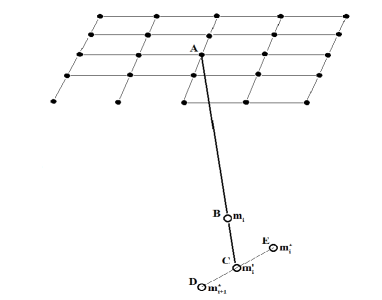
Figure 1. : Illustration of dipoles in a birth-move.

3 REVERSIBLE JUMP MCMC ALGORITHM

We now describe a reversible jump MCMC algorithm for the dipole model. First, we describe the within-model moves where the number of dipoles is fixed at $k$, i.e. there are no birth nor death moves.

3.1 Within model moves - Metropolis-Hastings algorithm

The Metropolis-Hastings algorithm was first described by Hastings (1970) as a generalization of the Metropolis algorithm, Metropolis et al. (1953). Denote the state vector for the model of $k$ dipoles as

$${\rm{\boldsymbol{\theta}}}=(\theta_{1},\theta_{2},...,\theta_{3k+2},\theta_{3k+3})={\rm{\bf\Theta}}_{k}=(\omega,\varphi,m,x_{1},y_{1},z_{1},...,x_{k},y_{k},z_{k}).$$

At step $t$ the state vector ${\boldsymbol{\theta}}={\boldsymbol{\theta}}^{(t)}$ and we wish to update it to a new state ${\rm{\bf\theta}}^{(t+1)}$. We generate a candidate ${\boldsymbol{\theta}}^{*}$ from candidate generating density $q({\boldsymbol{\theta}}^{*}|{\boldsymbol{\theta}}^{(t)})$, we then accept this point as the new state of the chain with probability $p_{a}({\boldsymbol{\theta}}^{(t)},{\boldsymbol{\theta}}^{*})$ given by

$$p_{a}({\boldsymbol{\theta}}^{(t)},{\boldsymbol{\theta}}^{*})=\text{min}\left\{1,\frac{\pi({\bf\tilde{H}}|{\boldsymbol{\theta}}^{*})\pi({\boldsymbol{\theta}}^{*})q({\boldsymbol{\theta}^{(t)}}|{\boldsymbol{\theta}}^{*})}{\pi({\bf\tilde{H}}|{\boldsymbol{\theta}^{(t)}})\pi({\boldsymbol{\theta}^{(t)}})q({\boldsymbol{\theta}}^{*}|{\boldsymbol{\theta}^{(t)}})}\right\}$$ (4)

where $\pi({\rm{\bf\tilde{H}}}|{\boldsymbol{\theta}})$ is the likelihood given by (3), $\pi({\boldsymbol{\theta}})$ is the prior density. If the proposal is accepted, we let the new state ${\boldsymbol{\theta}}^{(t+1)}={\boldsymbol{\theta}}^{*}$, otherwise ${\boldsymbol{\theta}}^{(t+1)}={\boldsymbol{\theta}}^{(t)}$. It is often more efficient to partition the state variable ${\boldsymbol{\theta}}$ into components and update these components one by one. This was the framework for MCMC originally proposed by Metropolis et al. (1953), and it is used in this work. For each component $\theta_{j}$, we take the normal density as the proposal density $q(\theta_{j}^{\ast}|\theta_{j}^{(t)})=f_{n}(\theta_{j}^{\ast}-\theta_{j}^{(t)}|0,\sigma_{j})$, where $f_{n}(.|0,\sigma_{j})$ is the normal density with zero mean and standard deviation $\sigma_{j}$. A sensible choice for the $\sigma_{j}$ values is to let $\sigma_{1}=\sigma_{2}=\sigma_{\omega}$ for the two common polar coordinates, $\sigma_{3}=\sigma_{m}$ for the common magnetic strength, and $\sigma_{4}=\sigma_{5}=...=\sigma_{3k+3}=\sigma_{xyz}$ for all the position coordinates.

3.2 Trans-dimensional moves

The reversible jump Markov chain Monte Carlo proposed by Green (1995) provides a framework for constructing reversible Markov chain samplers that jump between parameter spaces of different dimensions, thus permitting exploration of joint parameter and model probability space via a single Markov chain. As shown by Green (1995), detailed balance is satisfied if the proposed move from ${\rm{\bf\Theta}}_{i}$ to ${\rm{\bf\Theta}}_{j}$ is accepted with probability $\alpha=\min\left\{{1,\alpha_{i\to j}({\rm{\bf\Theta}}_{i},{\rm{\bf\Theta}}_{j})}\right\}$, with $\alpha_{i\to j}({\rm{\bf\Theta}}_{i},{\rm{\bf\Theta}}_{j})$ given by

$$\alpha_{i\to j}({\rm{\bf\Theta}}_{i},{\rm{\bf\Theta}}_{j})=\frac{\pi({\bf\tilde{H}}|{\rm{\bf\Theta}}_{j})r_{j\to i}({\rm{\bf\Theta}}_{j})\varphi_{j}({\rm{\bf{u}}_{j}}|{\rm{\bf{\beta}}_{j}})}{\pi({\bf\tilde{H}}|{\rm{\bf\Theta}}_{i})r_{i\to j}({\rm{\bf\Theta}}_{i})\varphi_{i}({\rm{\bf{u}}_{i}}|{\rm{\bf{\beta}}_{i}})}\left|\frac{\partial g_{i\to j}({\rm{\bf\Theta}}_{i},{\bf u}_{i})}{\partial({\rm{\bf\Theta}}_{i},{\bf u}_{i})}\right|$$ (5)

where $r_{i\to j}({\rm{\bf\Theta}}_{i})$ is the probability that a proposed jump from ${\rm{\bf\Theta}}_{i}$ to ${\rm{\bf\Theta}}_{j}$ is attempted, $\varphi_{i}(.)$ is a proposal density, and $\left|{\partial g_{i\to j}({\rm{\bf\Theta}}_{i},{\rm{\bf u}}_{i})/\partial({\rm{\bf\Theta}}_{i},{\rm{\bf u}}_{i})}\right|$ is the Jacobian of the deterministic mapping. Efficiency of RJ-MCMC depends on the choice of mapping function $g_{i\to j}$ and the proposal density $\varphi_{i}(.)$.

3.2.1 Birth move

Typically, a birth-move is from ${\rm{\bf\Theta}}_{k}$ to ${\rm{\bf\Theta}}_{k+1}$, i.e. in the above description we have $i=k$ and $j=k+1$. In order to have a reasonable acceptance rate for the birth move, we try to keep the change in the likelihood function from $\pi({\rm{\bf\tilde{H}}}|{\rm{\bf\Theta}}_{k})$ to $\pi({\rm{\bf\tilde{H}}}|{\rm{\bf\Theta}}_{k+1})$ to be small, i.e. the birth-move is designed in such a way that $\pi({\rm{\bf\tilde{H}}}|{\rm{\bf\Theta}}_{k})\approx\pi({\rm{\bf\tilde{H}}}|{\rm{\bf\Theta}}_{k+1})$. To achieve this small perturbation in likelihood function, instead of randomly adding a new dipole to the system, we replace one of the existing dipoles with two new dipoles. Ideally, the combined magnetic field produced by the two new dipoles should be very close to the magnetic field of the replaced dipole, at every measurement point ${\rm{\bf\tilde{x}}}_{n}$, $n=1,...,N$. It is analytically difficult to ensure this closeness of magnetic field at every measurement point ${\rm{\bf\tilde{x}}}_{n}$.

We can simplify the problem by ensure that the magnetic field produced by the new pair of dipoles is close to that of the old dipole at one key measurement point ${\rm{\bf\tilde{x}}}_{a}$, $1\leq a\leq N$. Typically the measurement points can be arranged in a horizontal ($\tilde{z}=\mbox{const})$ rectangular lattice$\tilde{x}_{\min}\leq\tilde{x}\leq\tilde{x}_{\max}$, $\tilde{y}_{\min}\leq\tilde{y}\leq\tilde{y}_{\max}$, as shown in Figure 1, and ${\rm{\bf\tilde{x}}}_{a}$ can be chosen to be located at the centre of the lattice.

In figure 1, the key measurement point ${\rm{\bf\tilde{x}}}_{a}$ is marked as A. Assuming the randomly chosen dipole ${\rm{\bf m}}_{i}$ is located at point B with coordinate vector ${\rm{\bf x}}_{i}$, we wish to find two locations near B such that the new pair of dipoles located at these two points will produce a combined magnetic field close to that of the old dipole ${\rm{\bf m}}_{i}$. Let the two new locations be E and D for the new dipoles ${\rm{\bf m}}_{i}^{\ast}$ and ${\rm{\bf m}}_{i+1}^{\ast}$, as shown in Figure 1.

Denote the vector $\overrightarrow{AB}=-{\rm{\bf r}}_{B,A}=-r_{B,A}{\rm{\bf\hat{r}}}_{B,A}$, where $r_{B,A}$ is the distance between A and B and ${\rm{\bf\hat{r}}}_{B,A}$ is the unit vector from B to A (from dipole to measurement point). Now extend $\overrightarrow{AB}$ to $\overrightarrow{AC}$ such that $\overrightarrow{AC}=-{\rm{\bf r}}_{C,A}=-\sqrt[3]{2}\times r_{B,A}{\rm{\bf\hat{r}}}_{B,A}$, i.e. let C be on the same line as $\overrightarrow{AB}$ and the length of $\overrightarrow{AC}$ is $\sqrt[3]{2}$ times that of the length of $\overrightarrow{AB}$. Now we put two dipoles $({\rm{\bf{m}^{\prime}}}_{i},{\rm{\bf{m}^{\prime}}}_{i})$ at the same location C.

We now can easily show that a pair of dipoles $({\rm{\bf{m}^{\prime}}}_{i},{\rm{\bf{m}^{\prime}}}_{i})$ co-located at C produce a combined magnetic field (all 3 components) at measurement point A identical to that of dipole ${\rm{\bf m}}_{i}$, given that all dipoles have the same strength $m$ and unit vector ${\rm{\bf\hat{m}}}$. Applying field equation (3) to dipole ${\rm{\bf m}}_{i}$ and measurement location $A$, we have

$${\bf H}({\bf m}_{i},{\bf r}_{B,A})=\frac{\mu_{0}m}{4\pi r^{3}_{B,A}}\left(3({\bf\hat{m}}\cdot{\bf\hat{r}}_{B,A})({\bf r}_{B,A}-{\bf\hat{m}})\right)$$ (6)

Similarly, applying field equation (3) to dipole ${\rm{\bf{m}^{\prime}}}_{i}$ and measurement location A, we have

$${\bf H}({\bf m}_{i}^{\prime},{\bf r}_{C,A})=\frac{\mu_{0}m}{4\pi r^{3}_{C,A}}\left(3({\bf\hat{m}}\cdot{\bf\hat{r}}_{C,A})({\bf r}_{C,A}-{\bf\hat{m}})\right)$$ (7)

Because $r_{C,A}=\sqrt[3]{2}\times r_{B,A}$ and ${\rm{\bf\hat{r}}}_{C,A}={\rm{\bf\hat{r}}}_{B,A}$, comparing (6) and (7) we obtain ${\rm{\bf H}}({\rm{\bf{m}^{\prime}}}_{i}^{,}{\rm{\bf r}}_{C,A})={\rm{\bf H}}({\rm{\bf m}}_{i},{\rm{\bf r}}_{C,A})/2$. Thus a pair of dipole $({\rm{\bf{m}^{\prime}}}_{i},{\rm{\bf{m}^{\prime}}}_{i})$ co-located at point C produce combined magnetic field at point A identical to the magnetic field produced by dipole ${\rm{\bf m}}_{i}$ located at B, provided all the three dipoles have a common strength $m$ and unit vector ${\rm{\bf\hat{m}}}$.

Therefore we propose the following birth-move procedure, assuming the key measurement point A is fixed throughout the MCMC iterations

1. Randomly remove a dipole ${\bf m}_{i}$ (located at B in Figure 1) .

2. Locate point C by extending the line from $\overrightarrow{AB}$ to $\overrightarrow{AC}$, so that C is on the same line as $\overrightarrow{AB}$ and $|\overline{AB}|=\sqrt[3]{2}|\overline{AC}|$;

3. Put two dipoles at location C;

4. Generate three independent random variables $dx$, $dy$, $dz$ from normal distribution $f_{n}(0,\sigma_{xyz})$;

5. Move one of the two dipoles from C to location E, such that $\overrightarrow{CE}={\rm{\bf i}}dx+{\rm{\bf j}}dy+{\rm{\bf k}}dz$. This new dipole is denoted as ${\rm{\bf m}}_{i}^{\ast}$ located at ${\rm{\bf x}}_{i}^{\ast}$ (point E in Figure 1);

6. Move the other dipole from C to location D, such that $\overrightarrow{CD}=-\overrightarrow{CE}$. This new dipole is denoted as ${\rm{\bf m}}_{i+1}^{\ast}$ located at ${\rm{\bf x}}_{i+1}^{\ast}$ (point D in Figure 1).

The random vector ${\rm{\bf u}}_{k}$ corresponding to the birth-move from ${\rm{\bf\Theta}}_{k}$ to ${\rm{\bf\Theta}}_{k+1}$ is identified as ${\rm{\bf u}}_{k}=(dx,dy,dz)$ with a single parameter $\beta_{k}=\sigma_{xyz}$, the standard deviation for the random walk of a dipole. Thus

$$\varphi_{k}({\rm{\bf u}}_{k}|{\rm{\bf\beta}}_{k})=f_{n}(dx|0,\sigma_{xyz})f_{n}(dy|0,\sigma_{xyz})f_{n}(dz|0,\sigma_{xyz}).$$

To find the Jacobian of the deterministic mapping, we first find the mapping function $g_{k\to k+1}({\rm{\bf\Theta}}_{k},{\rm{\bf u}}_{k})$

$$x_{i}^{\ast}=(1-c)\tilde{x}_{a}+cx_{i}+dx,\;\;\;y_{i}^{\ast}=(1-c)\tilde{y}_{a}+cy_{i}+dy,\;\;\;z_{i}^{\ast}=(1-c)\tilde{z}_{a}+cz_{i}+dz$$ (8)

$$x_{i+1}^{\ast}=(1-c)\tilde{x}_{a}+cx_{i}-dx,\;\;\;y_{i+1}^{\ast}=(1-c)\tilde{y}_{a}+cy_{i}-dy,\;\;\;z_{i+1}^{\ast}=(1-c)\tilde{z}_{a}+cz_{i}-dz$$ (9)

where $c=\sqrt[3]{2}$, from which we find the Jacobian to be $\left|{\partial g_{k\to k+1}({\rm{\bf\Theta}}_{k},{\rm{\bf u}}_{k})/\partial({\rm{\bf\Theta}}_{k},{\rm{\bf u}}_{k})}\right|=8c^{3}=16$. Assume the probability to propose the general birth move (as against a birth-move or a within-model move) is $p_{b}$, and we know the probability of choosing ${\rm{\bf m}}_{i}$ among the $k$ dipoles is $1/k$, so for the birth-move we have $r_{k\to k+1}({\rm{\bf\Theta}}_{k})=p_{b}/k$ and

$$\frac{1}{r_{k\to k+1}({\rm{\bf\Theta}}_{k})\varphi_{k}({\rm{\bf{u}}_{k}}|{\rm{\bf{\beta}}_{k}})}\left|\frac{\partial g_{k\to k+1}({\rm{\bf\Theta}}_{k},{\rm{\bf u}}_{k})}{\partial({\rm{\bf\Theta}}_{k},{\rm{\bf u}}_{k})}\right|=\frac{16k}{p_{b}f_{n}(dx|0,\sigma_{xyz})f_{n}(dy|0,\sigma_{xyz})f_{n}(dz|0,\sigma_{xyz})}$$ (10)

3.2.2 Death move

This is the reversal of the birth-move (still using Figure 1 as illustration):

1. Randomly select a pair of dipoles among the $k(k-1)/2$ pairs, delete them from the system, assuming that, without losing generality, the pair are ${\rm{\bf m}}_{j}({\rm{\bf x}}_{j})$ located at E and ${\rm{\bf m}}_{j+1}({\rm{\bf x}}_{j+1})$ located at D;

2. find the middle point C between E and D, as shown in Figure 1, and locate point B on the line $\overline{AC}$ so that $\left|{\overline{AC}}\right|=\sqrt[3]{2}\times\left|{\overline{AB}}\right|$.

3. Put one dipole $m_{j}^{\ast}({\rm{\bf x}}_{j}^{\ast})$ at location B, where ${\rm{\bf x}}_{j}^{\ast}$ is the coordinate of point B.

In the above one-for-two death-move, the only random number is from uniform $\left(1,k(k-1)/2\right)$. The probability of making the specific death-move is $r_{k+1}({\rm{\bf\Theta}}_{k+1})=2p_{d}/\left({k(k-1)}\right)$, where $p_{d}$ is the probability of attempting a general death-move. The mapping function $g_{k+1\to k}({\rm{\bf\Theta}}_{k+1},{\rm{\bf u}}_{k+1})$ is the inverse of the mapping function $g_{k\to k+1}({\rm{\bf\Theta}}_{k},{\rm{\bf u}}_{k})$.

3.2.3 Acceptance rates

Combining birth-move and death-move as described above, we obtain the following expressions for acceptance rates:

Birth-move acceptance rate

$$p_{a}({\rm{\bf\Theta}}_{k},{\rm{\bf\Theta}}_{k+1})=\text{min}\{1,\alpha_{k\to k+1}\}$$ (11)

$$\alpha_{k\to k+1}=\frac{32p_{d}\times\pi({\bf\tilde{H}}|{\rm{\bf\Theta}}_{k+1})}{p_{b}f_{n}(dx|0,\sigma_{xyz})f_{n}(dy|0,\sigma_{xyz})f_{n}(dz|0,\sigma_{xyz})(k-1)\times\pi({\bf\tilde{H}}|{\rm{\bf\Theta}}_{k})}$$ (12)

Death-move acceptance rate

$$p_{a}({\rm{\bf\Theta}}_{k+1},{\rm{\bf\Theta}}_{k})=\text{min}\{1,\alpha_{k+1\to k}\}$$ (13)

$$\alpha_{k+1\to k}=\frac{p_{b}f_{n}(dx|0,\sigma_{xyz})f_{n}(dy|0,\sigma_{xyz})f_{n}(dz|0,\sigma_{xyz})(k-1)\times\pi({\bf\tilde{H}}|{\rm{\bf\Theta}}_{k})}{32p_{d}\times\pi({\bf\tilde{H}}|{\rm{\bf\Theta}}_{k+1})}$$ (14)

4 PRELIMINARY RESULTS

We consider three cases: 1 - A bulky formation; 2 - A thin plate; 3 - Two objects. In each case we start with a single dipole, located at an arbitrary depth below the measured magnetic field, and with an arbitrary orientation and a fixed strength.

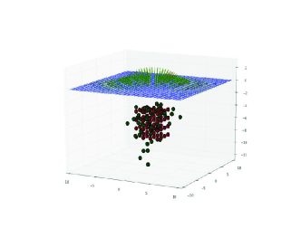
Figure 2. : Predicted dipoles and their vector fields for case 1.

Case 1. In this case the dipoles form a regular cube. Figure 2 shows a sample after 50000 simulations. In Figure 2, the red balls represent the true model, and green balls are the ’best’ prediction. The horizontal blue lattice indicates measurement points, and the lines originating from these points are the magnetic vectors with green corresponding to the green dipoles (the predicted dipoles) and red corresponding to the red diploes (the true model). As can be seen, on the whole, the inversed dipoles reasonably assemble the true model, with a few dipoles drifting to the deeper depth. The predicted magnetic vector field matches that of the true model very well - the green vectors and red vectors appear to be the same everywhere on the measurement lattice.

Case 2. In this case, the dipoles form a horizontal thin sheet, as shown by the blue balls in Figure 3. As seen in figure 3, the resulting dipoles are too much scattered vertically. Nevertheless, the horizontal scattering of the dipoles resemble the true model, and the resulting magnetic field vector matches the true vector field very well.

Case 3. In this case the dipoles form two separated identical cubes at a significantly different depths and horizontal locations. It can be seen there are still too many dipoles scattered in between the two objects, and already the fit between the predicted and measured magnetic vector fields are very good.

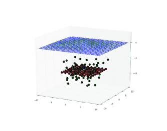
Figure 3. : Predicted dipoles and their vector fields for case 2.

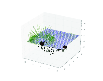
Figure 4. : Predicted dipoles and their vector fields for case 3.

The three test cases show that the present method is promising but some challenges remain. For a single cube-like object, the inverse is not too bad in terms of representing the overall shape of the object, although there seem to be always some dipoles scattered below the object. If the single object is a bit extreme, such as a horizontal thin sheet, the inverse cannot predict the depth resolution – it is too scattered vertically. For a more challenging problem of two objects located at different depth, the inverse tried hard to locate both, but with too many dipoles scattered in between.

In all the above cases the forward problem was well resolved – i.e. the predicted magnetic field agrees very well with measured field. This is typical in geophysical inversion – non-uniqueness or ill-conditioning is demonstrated in terms of large uncertainties in the prediction of depth.

5 CONCLUSIONS

We have proposed a reversible jump Markov chain Monte Carlo (RJ-MCMC) algorithm for both the magnetic vector and its gradient tensor to deal with this trans-dimensional inverse problem where the number of unknowns is one the unknowns. A special birth-death move strategy is designed to obtain a reasonable rate of acceptance for the RJ-MCMC sampling. Some preliminary results show the strength and challenges of the algorithm in inversing the magnetic measurement data. Although it is very difficult, if not impossible, to predict each individual dipole accurately, it is important to predict the cloud of dipoles accurately (e.g. uniformly distributed with the edges close to the true boundary). A different likelihood function or prior (in addition to new method) may be of help in this regard. As always, it is difficult to predict the depth of the object with reasonable certainty. Better ways are needed to locate multiple objects - with a clean break between two distinct objects, especially when they are located at very different depths.

Acknowledgement

This project was funded by the Capability Development Fund of CSIRO Earth Science and Resource Engineering.

References

- Anderssen and Seneta (1971) Anderssen, R. S. and E. Seneta (1971). A simple statistical estimation procedure for monte carlo inversion in geophysics. Pure and Applied Geophysics 91, VIII, 5–13.
- Anderssen et al. (1972) Anderssen, R. S., M. H. Worthington, and J. R. Cleary (1972). Density modelling by monte carlo inversion - i methodology. Geophys. J. R. astr. Soc. 29, 433–444.
- Bodin and Sambridge (2009) Bodin, T. and M. Sambridge (2009). Seismic tomography with the reversible jump algorithm. Geophys. J. Int. 178, 1411–1436.
- Green (1995) Green, P. (1995). Reversible jump mcmc computation and bayesian model determination. Biometrika 82, 711–732.
- Green (2003) Green, P. (2003). Trans-dimensional markov chain monte carlo. Highly Structured Stochastic Systems Chapter 6, 179–198.
- Hastings (1970) Hastings, W. (1970). Monte carlo sampling methods using markov chains and their applications. Biometrika 57, 97–109.
- Keilis-Borok and Yanovskaya (1967) Keilis-Borok, V. I. and T. B. Yanovskaya (1967). Inverse problems of seismology. Geophysics Journal 13, 223–34.
- Luo (2010) Luo, X. (2010). Constraining the shape of a gravity anomalous body using reversible jump markov chain monte carlo. Geophysical Journal International 180, 1067–1069.
- Malinverno and Leaney (2005) Malinverno, A. and W. S. Leaney (2005). Monte-carlo bayesian look-ahead inversion of walkaway vertical seismic profiles. Geophysical Prospecting 53, 689–703.
- Metropolis et al. (1953) Metropolis, N., A. W. Rosenbluth, M. N. Rosenbluth, A. H. Teller, and E. Teller (1953). Equations of state calculations by fast computing machines. J. Chem. Phys. 21, 1087–1091.
- Mosegaard and Tarantola (2002) Mosegaard, K. and A. Tarantola (2002). Probabilistic approach to inverse problems. International Handbook of Earthquake and Engineering Seismology Part A, 237–265.
- Sambridge et al. (2006) Sambridge, M., K. Gallagher, A. Jackson, and P. Rickwood (2006). Trans-dimensional inverse problems, model comparison and the evidence. Geophys. J. Int. 167, 528–542.