Continuous-time Modeling of Bid-Ask Spread and Price Dynamics in Limit Order Books

Abstract

We derive a continuous time model for the joint evolution of the mid price and the bid-ask spread from a multiscale analysis of the whole limit order book (LOB) dynamics. We model the LOB as a multiclass queueing system and perform our asymptotic analysis using stylized features observed empirically. We argue that in the asymptotic regime supported by empirical observations the mid price and bid-ask-spread can be described using only certain parameters of the book (not the whole book itself). Our limit process is characterized by reflecting behavior and state-dependent jumps. Our analysis allows to explain certain characteristics observed in practice such as: the connection between power-law decaying tails in the volumes of the order book and the returns, as well as statistical properties of the long-run spread distribution.

1 Introduction

Limit order book (LOB) models have recently attracted a lot of attention in the literature given their importance in modern financial markets and they are used as trading protocol in most exchanges around the world. For a brief review of worldwide financial markets that use LOB mechanism, see the first paragraph of Gould et al. [9]. As we shall discuss, the literature on price modeling based on LOB dynamics has mostly focused on one side of the order book, or price dynamics that are not fully informed by the LOB.

One of our main contributions is the construction of a continuous time model for the joint evolution of the mid price and the bid-ask spread (see Theorem 2 in Section 4). Such construction is informed by the full LOB dynamics, which we model as a multiclass queueing system (see Section 2). We endow the multiclass queue with characteristics that are inspired by common stylized features which are observed empirically in order book data, such as: very fast speed of orders relative to price changes, high cancellation rates, and power-law tails (see for example Sections 3 and 5). Some of these stylized features allow us to justify the use of certain asymptotic limits and weak convergence analyses which are applied to the LOB and ultimately give rise to our continuous time pricing model.

Another contribution that it is important to highlight is that our analysis sheds light on the connection between power-law tails which are present both in the distribution of orders inside the book, and also in the realized return distributions of price processes. The connection between these features, which are documented in the statistical literature (see Bouchard et al. [2]) are explained as a result of the statements obtained in Theorem 1 and Proposition 1 in Section 4. Basically the power-law tails arising from the distribution of returns in the price processes can be explained as a consequence of the power-law tails in the distribution of orders inside the book, the effect of cancellation policies, and the asymptotic regime under which LOBs operate.

We establish a one-to-one correspondence between the distribution of orders inside the book and the price-return distribution assuming a specific form of the cancellation policy (see Proposition 1 for the one-to-one correspondence and Assumption 1 for the form of the cancellation policy). We argue that such cancellation policy has qualitative features observed in practice. For example, we postulate higher cancellation rates for orders that are placed closer to the spread and lower cancellation rates for orders placed away from the spread (see the discussion at the end of Section 3.2). Further, we also argue that the cancellation rate that we postulate is such that, in statistical equilibrium, the probability at which a given order is executed before cancellation is roughly the same regardless of where the order is placed in book.

Although we believe that our cancellation policy is reasonable in some circumstances, more generally, our results are certainly useful to obtain insights into the form of cancellation used by market participants. This insight could be obtained by comparing the distribution of orders inside the book and the price return distribution relative to equation (1), which also contains the cancellation rates.

Furthermore, we also argue in Section 3.2.1 that a strong connection between distribution of orders inside the book and price-return distribution is to be expected in a different asymptotic regime, namely, that in which market and limit orders arrive at comparable speed, and constant cancellation rates per order across the book. We thus believe that our analysis provides significant evidence for such connection between these distributions.

We envisage our model to be useful in intra-day trading. Underlying the motivation behind the construction of our model is our belief that there is a significant amount of information in the order book which can be used to help describe the evolution of the price and bid-ask spread in the order of a few hours. At the same time, we recognize that it might be challenging in practice to keep track of the full LOB to describe price dynamics. Fortunately, as we demonstrate here, under the asymptotic regime that we utilize, implied by empirical observations, it is possible to keep track of the prices in continuous time using only a two dimensional Markov process. Our continuous-time pricing model can be calibrated, for example, from the historical data of the distribution of limit orders inside the book, and then fine tuned (through an additional parameter which we call the patience ratio, $c_{p}$) again based on historical price return distribution data (see for example the discussion in Section 5 involving Empirical Observation 3). Therefore, we are able to use the information on the order book in a meaningful, yet relatively simple, way to inform the future evolution of prices. Moreover, as we shall illustrate, using simulated data, our final model captures empirical features observed in practice (see Section 5).

Let us discuss briefly the elements that distinguish our work from previous contributions. As we indicated earlier, we built our model from a multiclass queueing system. Queueing theory provides a natural environment for the study of LOB dynamics at a microstructure level. Consequently, it is no surprise that there is a fast growing literature that leverages off the use of queueing theory in order to analyze LOBs and the corresponding price dynamics. Cont et al. [6] introduces birth-death queueing model similar to our prelimit model discussed in Section 2. They demonstrate that this model can lead to computable conditional probabilities of interest in terms of Laplace transforms studied in queueing theory. A scaling is introduced in a subsequent paper Cont and Larrard [5] in which a continuous-time process is derived for price dynamics, but there the authors assume that price dynamics only depend on best bid and ask quotes. In contrast, we derive a two dimensional Markovian process for the best bid and best ask quotes from the whole order book model. As a result, we arrive at a limiting process which is different from that of Cont and Larrard [5]. In Maglaras et al. [15], queueing models are used to address the problem of routing of orders in a fragmented market with different books. More recently, Lakner et al. [14]. discuss a one sided order book and track the whole process using measure-valued characteristics. Although they analyze the system in a high-frequency trading environment their scaling does not appear to highlight the role of the cancellations relative to what occurs in the markets, in which a large proportion of the orders are actually cancelled. In contrast we not only consider the two sides of the book, but we believe our scalings better preserve the empirical features observed in practice.

As mentioned earlier, we use multiscale analysis, which allows us to replace most of the stochasticity in the book by steady-state dynamics. The paper by Sowers et al. [18] also takes advantage of multiscale analysis, but their model is not purely derived from the microstructure characteristics at the level of arrivals of limit and market orders and therefore the ultimate model is different from the one we obtain. A recent paper by Horst and Paulsen [12] provides a law of large numbers description of the order book and the price process, which is in the end deterministic and therefore also different in nature to the stochastic model we derive here. Nevertheless, we feel that the spirit of Horst and Paulsen [12] is close to the work we do here.

A related literature on model building for order book dynamics relates to the use of self-exciting point processes. The approach is somewhat related to the queueing perspective, although the models are more aggregated than the ones we consider in this paper; for example, in Zheng et al. [20] a model is discussed that considers only best bid and ask quotes but with a self-exciting mechanism with constraints (see also Cartea et al. [4], Muni Toke [16] and the references therein) for more information on self-exciting processes in high-frequency trading.

This manuscript is organized as follows. In Section 2 we discuss the pre-limit model underlying the LOB dynamics. In Section 3 we discuss some empirical observations that inform the construction of certain approximations in our model which in particular allow to connect the price increments and the distribution of orders in the LOB. In Section 4 we present our asymptotic scalings and our continuous time price model. Finally, in Section 5 we discuss how, using simulated data, our final model captures empirical features observed in practice.

2 Basic Building Blocks

Ultimately, our goal is to construct a continuous time model for the joint evolution of the mid price and the bid-ask spread, which is informed by the whole order book dynamics in such a way that key stylized features are captured. In the end our model will be obtained as an asymptotic limit which is informed by stylized features observed empirically. We first discuss the building blocks of our model in the prelimit.

The building blocks of our model are consistent with prevalent limit order book models that describe the interactions between order flows, market liquidity and price dynamics, such as in Bouchard et al. [2] Cont et al. [6]. In most existing models, the arrival rate of limit orders corresponding, say, to a given price is given as a function of the distance between such given price and the best price of all present limit orders of the same type (buy or sell).

The best price of all limit sell (and buy) orders is called the ask (and bid) price and is usually denoted by $a(t)$ (and $b(t)$) at time $t$. However, as observed in recent empirical data, due to the growing popularity of algorithmic trading, limit orders are put and canceled without being executed at high frequency, especially at positions between the best ask or bid prices (fleeting orders). Therefore, the continuous observation of the best bid-ask prices may result in a process with too much “noise” due to variability caused by cancellations of such fleeting orders.

Instead, we shall construct our continuous time model by looking at the prices only at time at which an actual trade occurs; we call these quantities prices per trade. We believe that this is the natural time scale at which track the evolution of the LOB in order to derive a continuous time price process.

The relation between the price-per-trade process $(\bar{a}(\cdot),\bar{b}(\cdot))$ and $(a(\cdot),b(\cdot))$ is as follows. Suppose $\{t_{k}:k\geq 1\}$ are the arrival times of market orders (on both sides), then $(\bar{a}(t),\bar{b}(t))=(a(t_{k}),b(t_{k}))$ if $t_{k}\leq t<t_{k+1}$. As indicated, intuitively, we can think of $(\bar{a}(\cdot),\bar{b}(\cdot))$ as a mechanism to filter out the noise made by fleeting orders in the prelimit process $(a(\cdot),b(\cdot))$. The model that we consider in the prelimit is described as follows.

Model Dynamics and Notation:

1. Limit orders or market orders arrive one at a time (i.e. there are no batch arrivals).

2. Arrivals of limit buy orders and of sell orders are modelled as two independent Poisson processes with equal rate $\lambda$.

3. Arrivals of market buy orders and of sell orders are modelled as two independent Poisson processes with equal rate $\mu$.

4. Let $\{t_{k}:k\in\mathbb{Z^{+}}\}$ be the arrival times of the market orders (either buy or sell, so these are the arrivals of a Poisson process with rate $2\mu$).

5. The prices take values on the lattice $\{i\delta:i\in\mathbb{Z^{+}}\}$ and we observe their change at time lattice points $\{t_{k}:k\in\mathbb{Z^{+}}\}$. The parameter $\delta$ is called the tick size and in the sequel we will specify an asymptotic relationship between $\delta$ and the frequency of arrival times of orders.

6. At time $t$, the ask price $a(t)$ (the bid price $b(t)$) equals the minimum (maximum) of prices of all limit sell (buy) orders on the order book at time $t$.

7. For $t_{k}\leq t<t_{k+1}$, an order placed at a relative ask price equal to $i\delta$ at time $t$ implies that the order is posted for ask price equal to $a\left(t_{k}\right)+i\delta$. Similarly, a relative bid price equal to $i\delta$ at time $t$ implies an absolute bid price equal to $b\left(t_{k}\right)-i\delta$.

8. For $t_{k}\leq t<t_{k+1}$, upon its arrival at time $t$, a limit buy (and sell) order sits at a relative price equal to $i\delta$ with probability $p(i\delta;\bar{a}(t_{k}),\bar{b}(t_{k}))$. In particular, $p(i\delta;a,b)=0$ for all $i\delta\geq-(a-b)/2$ so that the incoming limit buy and sell orders do not overlap with each other.

9. An order that right after time $t_{k}$ sits at a relative (buy or sell) price equal to $i\delta$ is cancelled at rate $\alpha(i\delta;\bar{a}(t_{k}),\bar{b}(t_{k}))$ during the time interval $[t_{k},t_{k+1})$.

10. A market order immediately transacts with any of the best matching limit orders in the order book upon its arrival.

Remark: We can actually weaken the assumption described in item 1. above to allow market orders arriving in batches as long as the size of incoming market order is less than the volume of standing limit orders at the best quote.

In our model, the ask and bid sides are two separate multi-class single-server queues with exponentially distributed times between transition of events (i.e. Markovian queues). On each side, the limit orders can be view as customers that are divided into different classes according to their relative prices (i.e. number of ticks to the best price). The class with lower relative price has higher priority. The market orders play the role of the server, as each of them causes a departure of a limit order from the best tick price. In other words, limit orders are served at the same rate as the arrival rate of market orders and the market orders pick customers from the non-empty class with the highest priority.

It is important to note that between the arrivals of two consequent market orders, the dynamic of the limit order book is equivalent to a set of independent infinite-server systems. One such infinite-server system for each class in each of the sides (buy and sell) of the order book. The “service rate” of each such infinite server system is equal to the cancellation rate of the corresponding class.

We now proceed to develop the main ingredients of our model using stylized features that are prevalent in market data.

3 Empirical Observations, Price, and LOB’s Distributions

We now discuss several empirical features that motivate the asymptotic regime that we consider. In particular, these observations will help us inform the asymptotic distribution of the price increments in intermediate time scales (order of several seconds).

3.1 Empirical Observations and Distribution of Price Increments

Empirical Observation 1: Multi-Scale Evolution of Limit Order Flows and the Occurrence of Trades . Table 1 is a sample from the descriptive statistics of TAQ data from Cont et al. [7]. In particular, we would like to hight the contrast between the daily number of updates, which include the submission, cancellation and transactions of limit orders at the best quote, and the daily number of trades (transactions). Since each market order causes a transaction of limit orders, the fact that the daily number of updates of limit orders at the best quote is much bigger than that of trades indicate that the evolution of limit orders is much more frequent than the arrivals of market orders in the limit order book. Moreover, such difference is prevalent in both high-liquidity stocks (such as Bank of America) and low-liquidity stocks (such as CME Group). We will adopt the relative fast speed of the limit order flows relative to market order flow (or occurrences of trade) in our asymptotic regime.

Table 1: Daily average of 50 randomly chosen stocks in NYSE over 21 trading days in April 2010.

	Daily Number of best quote updates	Daily number of trades
Bank of America	$1529395$	$15008$
CME Group	$38504$	$1412$
Grand mean	$223132$	$4552$

Empirical Observation 2: Fleeting Orders and High Cancellation Rate.

Due to the prevalence of algorithmic trading in these days, the cancellation rate of limit orders has increased dramatically over recent years. Among recent studies on the Nasdaq INET data, Hasbrouck and Saar [10] compares the data from year 1990, 1999 and 2004 and find that the cancellation rate has increased dramatically, while Hautsch and Huang [11] finds that about $95\%$ of the limit orders are canceled in the 2010 data as shown in Table 2.

Table 2: Percentage of limit orders that are canceled without (partial) execution for 10 stocks on NASDAQ. Samples are collected in October 2010, covering 21 trading days.

GOOG	ADBE	VRTX	WFMI	WCRX	DISH	UTHR	LKQX	PTEN	STRA
97.52	92.57	93.82	95.25	92.83	94.56	95.54	96.62	91.62	95.57

As suggested by this empirical work, the high cancellation rate can be attributed to the large proportion of “fleeting” limit orders which are usually put inside the spread and then canceled immediately if not executed. For example, Hautsch and Huang [11] reports that in 2010 Nasdaq data the mean inter-arrival time of market orders is about 7 seconds while the mean cancellation rate of limit orders inside the spread is less than 0.2 seconds. However, limit orders deep outside the spread are more patient. We will assume that the arrival rates and cancellation rates are substantially higher than the arrival rates of market orders in our model.

Recall that $\{t_{k}:k\geq 1\}$ is the sequence of arrival times of market orders (on both sides). We now discuss the distribution of the ask price-per-trade increment $(\bar{a}(t_{k+1})-\bar{a}(t_{k}))$. Similar results on the distribution of the bid price-per-trade increment $(\bar{b}(t_{k+1})-\bar{b}(t_{k}))$ follow by symmetry.

Note that the following identity of events holds

$$\{\bar{a}(t_{k+1})-\bar{a}(t_{k})\geq i\delta\}=\{\text{The queues at relative prices lower than }i\delta\text{ are all empty at time }t_{k+1}\}.$$

Let

$$\theta(i\delta;a,b)=P_{\pi}(\text{the queues at relative tick prices lower then }i\delta\text{ are all empty}),$$

where $\pi$ is the stationary distribution of the underlying infinite server queues associated to each class (which are all independent). The $i$-th queue has arrival rate $\lambda p(i\delta;\bar{a}(t_{k}),\bar{b}(t_{k}))$ and cancellation rate $\alpha(i\delta;\bar{a}(t_{k}),\bar{b}(t_{k}))$. It is known that the stationary distribution of an infinite server queue with arrival rate $\lambda p(i\delta;\bar{a}(t_{k}),\bar{b}(t_{k}))$ and service rate $\alpha(i\delta;\bar{a}(t_{k}),\bar{b}(t_{k}))$ is Poisson with parameter $\lambda p(i\delta;\bar{a}(t_{k}),\bar{b}(t_{k}))/\alpha(i;\bar{a}(t_{k}),\bar{b}(t_{k}))$, therefore we have that

$$\theta(i\delta;\bar{a}(t_{k}),\bar{b}(t_{k}))=\exp\left(~{}~{}-\sum_{j\delta\geq-(\bar{a}(t_{k})-\bar{b}(t_{k}))/2}^{i-1}\frac{\lambda p(j\delta;\bar{a}(t_{k}),\bar{b}(t_{k}))}{\alpha(j\delta;\bar{a}(t_{k}),\bar{b}(t_{k}))}\right).$$ (1)

As $\lambda>>\mu$ is large, suggested by Empirical Observation 1, and $\alpha(\cdot)>>\mu$ as suggested by the Empirical Observation 2, we can typically approximate the distribution of the queue lengths at time $t_{k+1}$ (given the state of the system at time $t_{k}$) by the associated steady-state distribution of the queues. More precisely, we expect the approximation $P(\bar{a}(t_{k+1})-\bar{a}(t_{k})\geq i\delta|\bar{a}(t_{k}),\bar{b}\left(t_{k}\right))\approx\theta(i\delta;\bar{a}(t_{k}),\bar{b}\left(t_{k}\right))$ to hold. This heuristic is made rigorous in the following theorem, the proof, which is given in Section 6.1, is based on the so-called stochastic averaging principle, see Kurtz [13]. We use $D[0,\infty)$ to denote the space of right continuous with left limits functions from $[0,\infty)$ to $\mathbb{R}$ endowed with the Skorokhod $J_{1}$ topology (see Billingsley [1] for reference).

Theorem 1.

Consider a sequence of LOB systems indexed by $n$. In the $n$-th system, the total number of orders in the order book is given by $q_{n}=q<\infty$, the distribution of these orders in the order book is assumed to satisfy $\bar{a}_{n}\left(0\right)=a_{n}\left(0\right)=\bar{a}$ and $\bar{b}_{n}(0)=b_{n}\left(0\right)=\bar{b}$. We assume that the arrival rate of market orders satisfies $\mu_{n}=\mu$ and the distribution of incoming limit orders is $p_{n}(\cdot;\cdot,\cdot)=p(\cdot;\cdot,\cdot)$ (i.e. constant along the sequence of systems). Suppose there exists a sequence of positive number $\{\xi_{n}:n\geq 1\}$ such that $\lambda_{n}=\xi_{n}\lambda$, $\alpha_{n}(\cdot)=\xi_{n}\alpha(\cdot)$ and $\xi_{n}\rightarrow\infty$ as $n\rightarrow\infty$. We also assume the regularity condition that for any $(a,b)\in\mathbb{Z}^{2}$

$$\lim_{i\rightarrow\infty}\theta(i\delta;a,b)=0.$$ (2)

Then the corresponding price process $(\bar{a}_{n}(\cdot),\bar{b}_{n}(\cdot))$ converges weakly in $D[0,\infty)$ to a pure jump process $(\hat{a}(\cdot),\hat{b}(\cdot))$. The process $(\hat{a}(\cdot),\hat{b}(\cdot))$ jumps at time corresponding to the arrivals of a Poisson process with rate $2\mu$. The size of the jumps are not independent, in particular, if $t$ is a jump time, then the jump size at $t$ is a random vector following the the distribution

$$P\left(\hat{a}(t)-\hat{a}(t-)=i\delta,\hat{b}(t)-\hat{b}(t-)=j\delta~{}|\hat{a}(t-),\hat{b}(t-)\right)$$

$$= [\theta(i\delta;\hat{a}(t-),\hat{b}(t-))-\theta((i+1)\delta;\hat{a}(t-),\hat{b}(t-))]\times[\theta(j\delta;\hat{a}(t-),\hat{b}(t-))-\theta((j+1)\delta;\hat{a}(t-),\hat{b}(t-))].$$

Remark: The regularity condition (2) not only is quite natural, but it can be easily verified in terms of $p\left(i\delta;a,b\right)$ and $\alpha\left(i\delta;a,b\right)$ because there is an explicit formula for $\theta\left(i\delta;a,b\right)$ given below in equation (1).

It is important to note that in the previous result we have held the arrival rates of market orders constant, so this result simply describes the price processes at times scales corresponding to the inter-arrival times of market orders (i.e. in the order of a few seconds according to the representative date discussed earlier). In Section 4 we shall introduce a scaling that will allow us to consider the process in longer time scales (several minutes or longer) by increasing the arrival rate of market orders.

Theorem 1 can be extended without much complications to include more complex dynamics in the arrivals of the market orders. For instance, one way to extend our model is to allow traders to post market orders depending on the current bid-ask price. This modification can be introduced as thinning procedure to the original Poisson process with rate $2\mu$, the thinning parameter might depend on the observed bid-ask price $(a(\cdot),b(\cdot))$. Other examples of the interactions between market participants that can be included in our model extensions are correlation between the buying and selling sides and dependence between arrival rate of market orders and the spread width.

3.2 Connecting Distribution of Price Increments and LOB’s Distributions

We now will argue how Theorem 1 allows us to provide a direct connection between the increment distribution of the price-per-trade process and the distribution of orders in the LOB. We believe that this connection, although simple, is quite remarkable because it forms the basis behind our idea of using information in the LOB to predict the evolution of prices.

Let us assume the following form for the cancellation rate.

Assumption 1.

$$\alpha(i\delta;\bar{a}(t_{k}),\bar{b}(t_{k}))=\frac{\lambda}{c_{p}}\cdot\frac{p(i\delta;\bar{a}(t_{k}),\bar{b}(t_{k}))}{log(1-\sum_{j\leq i-1}p(j\delta;\bar{a}(t_{k}),\bar{b}(t_{k})))-log(1-\sum_{j\leq i}p(j\delta;\bar{a}(t_{k}),\bar{b}(t_{k})))},$$ (3)

where $c_{p}>0$ is a constant we call the patience ratio of limit orders and we will see in a moment that it plays an important role in the connection between the distributions of limit order flow and price returns.

Under this assumption, by simple algebra in (1), we have the following result.

Proposition 1.

$$\theta(i\delta;\bar{a}(t_{k}),\bar{b}(t_{k}))=(1-\sum_{j\leq i-1}p(j\delta;\bar{a}(t_{k}),\bar{b}(t_{k})))^{c_{p}},$$ (4)

Since $\theta(\cdot;a,b)$ is the tail of price return and $1-\sum_{j\leq\cdot}p(j;a,b)$ is the tail of the relative price of incoming limit orders. Proposition 1 indicates that the price return inherits some statistical properties of the distribution of limit order flow on the order book. In real market data, power-law tails are reported in both the relative price of limit orders and the mid-price return as discussed in the next subsection. In our model, given that the distribution of the limit order flow $p(\cdot;\bar{a},\bar{b})$ has a power-law with exponent $v$, in other words, $\bar{F}^{c_{p}}(i\delta)=\sum_{j\geq i}p(j\delta;\bar{a},\bar{b})\approx(c_{1}i\delta)^{-v}$. Then, as a direct consequence of (4), we have $P(\hat{a}(t)-\hat{a}(t-)\geq i\delta|\bar{a},\bar{b})\approx(c_{1}i\delta)^{-c_{p}v}$ and therefore the price returns also follows a power law but with different exponent $c_{p}v$.

For $c_{p}>1$, our model recovers an interesting phenomenon in real market that the price return has a thinner tail than the relative price of limit orders as reported in Bouchard et al. [2]. Besides, in our model when the limit orders are more patient ($c_{p}$ increases), the price return has a thinner tail. This is consistent with the fact that price volatility decreases when the market has more liquidity supply (since the limit orders stand longer in the order book as $c_{p}$ increases).

We shall put some remarks on our Assumption 1 on the cancellation rate of limit orders. Although this assumption is made for mathematical tractability and because we did not find enough data to develop an empirical-based model, it is consistent with empirical observations to some level. In particular, under Assumption 1, the cancellation rate is decreasing with respect to the relative price $i\delta$ as is reported in Gould et al. [9] and the references therein. To see why $\alpha(\cdot;a,b)$ is decreasing, let’s assume that $p(i\delta;a,b)\leq A\delta$ for some constant $A>0$. Since for any fixed $h>0$ and $x>0$ small enough, $x/(\log(a+x)-\log(a))\approx a$, we have

$$\alpha(i\delta;a,b)\approx\frac{\lambda}{c_{p}}(1-\sum_{j\leq i-1}p(j\delta;a,b))$$

when $\delta$ is small enough and hence it is decreasing in $i\delta$.

Moreover, when $c_{p}=1$, $\theta(\cdot;a,b)=1-\sum_{j\leq i-1}p(j\delta;a,b)$. In this case, $\theta(\cdot;a,b)$ is approximately proportional to $\alpha(\cdot;a,b)$, which implies that the impatience level of a standing limit order at position $i\delta$ (namely $\alpha\left(i\delta;a,b\right)$) is proportional to its rate of execution as observed by the arriving market orders (namely $\mu\theta\left(i\delta;a,b\right)$). So, the probability that a given limit order in equilibrium at position $i\delta$ gets executed before cancellation is equal to $\mu\theta\left(i\delta;a,b\right)/(\alpha\left(i\delta;a,b\right)+\mu\theta\left(i\delta;a,b\right))\approx\mu/(\lambda+\mu)$. Consequently, in this sense all limit orders have roughly the same probability of execution in equilibrium.

3.2.1 Connecting Distribution of Price Increments and LOB’s Distributions in Other Regimes

We close this section by briefly discussing another asymptotic regime. Suppose that one assumes that the cancellation rate per order at relative price $i\delta$ equals $\alpha\left(i\delta,a,b\right)=\alpha$ (constant) – see for example Cont et al. [6]. Then one can check that the stationary distribution of the multi-class queues becomes,

$$\theta\left(i\delta,a,b\right)=\left(\sum_{l=0}^{\infty}\prod_{k=1}^{l}\frac{\lambda F\left(i\delta,a,b\right)}{\mu+k\alpha}\right)^{-1}.$$ (5)

So, if $\lambda_{n},\mu_{n}\rightarrow\infty$ in such a way that $\lambda_{n}/\mu_{n}\rightarrow c^{\prime}$ as $n\rightarrow\infty$ and $\alpha_{n}/\lambda_{n}\rightarrow 0$, then we obtain

$$\theta\left(i\delta,a,b\right)\approx\bar{F}\left(i\delta,a,b\right)/c^{\prime},$$

and arrive at the same conclusion as in Proposition 1 which $c_{p}=1$. We therefore believe that the sort of relationship that we have exposed via Proposition 1 between the return distribution and the distribution of orders in the book might be relatively robust. Under the assumption that $\lambda_{n}/\mu_{n}\rightarrow c^{\prime}$, there is no stochastic averaging principle such as discussed in Theorem 1. However, one can obtain a limiting price process with price increment distributed as (5) by observing the LOB and the price in suitably chosen discrete time intervals.

4 Continuous Time Model

We write $\bar{s}(t)=\bar{a}(t)-\bar{b}(t)$ to denote the bid-ask spread per-trade at time $t$. We shall develop a stochastic model for the price-spread dynamics in longer time scale (order of several minutes or more). The model will be a jump-diffusion limit of the discrete price-spread processes as given in Section 2.

We will now introduce the distribution of relative prices in the LOB, $p(\cdot;\bar{a}(t_{k}),\bar{b}(t_{k}))$. We shall impose our assumptions directly on $\theta(\cdot;\bar{a}(t_{k}),\bar{b}(t_{k}))$ because we can go back and forth between $\theta(\cdot;\bar{a}(t_{k}),\bar{b}(t_{k}))$ and $p(\cdot;\bar{a}(t_{k}),\bar{b}(t_{k}))$ directly via (4). We shall consider a sequence of limit order books indexed by $n$ and their ask-bid (per-trade) price process $\{(\bar{a}^{n}(\cdot),\bar{b}^{n}(\cdot))\}$. The dynamic of $(\bar{a}^{n}(\cdot),\bar{b}^{n}(\cdot))$ is characterized by the arrival rate of market orders and the price increments. In turn, the price increments will be defined in terms of auxiliary (spread-dependent) random variables denoted by $\Delta_{a}^{n}\left(\bar{s}^{n}(t_{k})\right)$ for the ask price process and $\Delta_{b}^{n}\left(\bar{s}^{n}(t_{k})\right)$ for the buy price process. For simplicity in the notation, we often write $\Delta_{a}^{n}\left(t_{k}\right)$ instead of $\Delta_{a}^{n}\left(\bar{s}^{n}(t_{k})\right)$ (similarly for $\Delta_{b}^{n}\left(t_{k}\right)$). We will assume that both $\Delta_{a}^{n}\left(t_{k}\right)$ and $\Delta_{b}^{n}\left(t_{k}\right)$ have the same distribution given the spread-per trade, so we simply provide the description for $\Delta_{a}^{n}\left(t_{k}\right)$ in our following assumption which is motivated by the Empirical Observation 3.

Assumption 2.

(Price return distribution) First define,

$$\Delta_{a}^{n}\left(\bar{s}^{n}(t_{k})\right)=(1-I_{k}^{a})\cdot(-1)^{R_{k}^{a}}[U_{k}^{a}/(\sqrt{n}\delta)]\delta+I_{k}^{a}[\bar{s}^{n}(t_{k})V_{k}^{a}/(2\delta)]\delta$$ (6)

where:

i) $I_{k}^{a}$ is Bernoulli with $P(I_{k}^{a}=1)=q$ for some $q>0$,

ii) $U_{k}^{a}$ is a random variable with support on $[0,\xi]$ for $\xi\in(0,\infty)$.

iii) $R_{k}^{a}$ is Bernoulli with $P(R_{k}^{a}=1)=(1+2\beta/\sqrt{n})/2$ for some $\beta>0$,

iv) $V_{k}^{a}$ is a continuous random variable so that $P(V_{k}^{a}\geq-1)=1$.

v) the random variables $I_{k}^{a}$, $U_{k}^{a}$, $R_{k}^{a}$ and $V_{k}^{a}$ are independent of each other (independence is assumed to hold across $k$ and for the superindices $a,b$).

Then we let

$$\begin{cases}\bar{a}^{n}(t_{k+1})=\bar{a}^{n}(t_{k})+\Delta_{a}^{n}\left(\bar{s}(t_{k})\right)\vee([-\bar{s}^{n}(t_{k})/(2\delta)]\delta),\\ \bar{b}^{n}(t_{k+1})=\bar{b}^{n}(t_{k})-\Delta_{b}^{n}\left(\bar{s}(t_{k})\right)\vee([-\bar{s}^{n}(t_{k})/(2\delta)]\delta),\end{cases}$$ (7)

and this is equivalent to assuming

$$\theta(i\delta,\bar{a}^{n}(t_{k}),\bar{b}^{n}(t_{k}))=P\left(\Delta_{a}^{n}\left(\bar{s}(t_{k})\right)\vee([-\bar{s}^{n}(t_{k})/(2\delta)]\delta)\geq i\delta\right).$$

Remarks:

1. The first term $(1-I_{k}^{a})\cdot(-1)^{R_{k}^{a}}[U_{k}^{a}/(\sqrt{n}\delta)]\delta$ captures limit orders tend to cluster close to their respective best bid or ask prices; the parameter $(1-q)\in\left(0,1\right)$ can represents the proportion of orders that are concentrated around the best bid or ask price. Since, as observed earlier, these correspond to a substantial proportion of the total number of orders placed, we might choose $q\approx 0$.

2. The second term $I_{k}^{a}[\bar{s}^{n}(t_{k})V_{k}^{a}/(2\delta)]$ captures the limit orders that are put far away from the current bid or ask price. In Section 5, we shall choose $V_{k}^{a}$ to have a density $f_{V}$ with a power-law decaying tails which are consistent with empirical observations (see Empirical Observation 3). We also postulate a multiplicative dependence on $\bar{s}^{n}(t_{k})$ to capture the positive correlation between size of spread and variability in return distribution as reported in (Bouchard et al. [3]).

3. Recall that the most aggressive price ticks that are allowed in our pre-limit model assumptions are at the mid price; this results in the cap $\vee([-\bar{s}^{n}(t_{k})/(2\delta)]\delta)$ appearing in (7), which consequently yields $\bar{a}^{n},\bar{b}^{n}$.

4. The asymmetry in the distribution of $R_{k}^{a}$ allows us to introduce a drift term in the spread, which will be useful to induce the existence of steady-state distributions. We will validate certain features of the steady-state distribution of our model vis-a-vis statistical evidence in Section 5.

In addition, we impose the following assumptions on time and space scalings, which are consistent with Empirical Observations 1 and 2. In order to carry out a heavy traffic approximation, we consider a sequence of LOB systems indexed by $n\in\mathbb{Z}^{+}$, such that in the $n$-th system:

Assumption 3.

(Time and Space Scale)

1. The arrival rate of market orders on each side $\mu_{n}=n\mu$;

2. Tick size $\delta_{n}\longrightarrow 0$ so that either $\delta_{n}=o\left(n^{-1/2}\right)$ or $\delta_{n}=n^{-1/2}$.

3. We assume that $q_{n}=\gamma/n$ for some $\gamma>0$.

In order to explain our scaling, note that the number of jumps, corresponding to the component involving $V_{k}^{a}$ in (6) is Poisson with rate $\gamma\mu$ so Condition 1 of Assumption 3 helps us capture jump effects in the limit. The scaling that we consider implies the existence of two types of arriving limit orders, one type that arrives more frequently than the other, see Assumption 3, part 3. in connection to Assumption 2, part i). This scaling feature, together with the fact that the probability of an order being executed is roughly constant across the book (as discussed at the end of Section 3.2) induces a much higher cancellation rate close to the spread, which is consistent with empirical findings.

Now we are ready to state our result on the spread and price dynamics informed by the limit order book.

Theorem 2.

For the $n$-th system, let $\bar{s}^{n}(t)=\bar{a}^{n}(t)-\bar{b}^{n}(t)$ be the spread process and $\bar{m}^{n}(t)=\bar{a}^{n}(t)+\bar{b}^{n}(t)$ be twice of the mean price. Suppose $(\bar{s}^{n}(0),\bar{m}^{n}(0))=(s_{0},m_{0})$. Then, under Assumptions 1-4, the pair of processes $(\bar{s}^{n},\bar{m}^{n})\in D([0,\infty),\mathbb{R}^{+}\times\mathbb{R})$ converges weakly to $(\bar{s},\bar{m})\in D([0,\infty),\mathbb{R}^{+}\times\mathbb{R})$ with $(\bar{s}(0),\bar{m}(0))=(s_{0},m_{0})$ such that

$$\begin{cases}d\bar{s}(t)&=-\eta dt+dW_{a}(t)+dW_{b}\left(t\right)+\bar{s}\left(t_{-}\right)dJ_{1}(t)/2+\bar{s}\left(t_{-}\right)dJ_{2}(t)/2+dL(t),\\ d\bar{m}(t)&=dW_{a}(t)-dW_{b}\left(t\right)+\bar{s}\left(t_{-}\right)dZ_{1}(t)/2-\bar{s}\left(t_{-}\right)dZ_{2}(t)/2.\end{cases}$$ (8)

Here,

1. $\eta=2\mu\beta E\left(\left[U_{1}^{a}\right]\right)=2\mu\beta E\left(\left[U_{1}^{b}\right]\right)$ if $\delta_{n}=n^{-1/2}$, and $\eta=2\mu\beta E\left(U_{1}^{a}\right)=2\mu\beta E\left(U_{1}^{b}\right)$ for $\delta_{n}=o(n^{-1/2})$.

2. $W_{a}$ and $W_{b}$ are two independent Brownian motions, each with zero mean and variance rate $\sigma^{2}=\mu E(\left[U_{j}^{a}\right]^{2})=$ $\mu E(\left[U_{j}^{b}\right]^{2})$ if $\delta_{n}=n^{-1/2}$, and $\sigma^{2}=\mu E((U_{j}^{a})^{2})=\mu E((U_{j}^{b})^{2})$ for $\delta_{n}=o(n^{-1/2})$.

3. $J_{1}$ and $J_{2}$ are two i.i.d. compound Poisson processes with constant jump intensity $\gamma\mu$ and the jump density distribution given by the density of $V_{1}^{a}$.

4. $\bar{s}(t)\geq 0$ and $L(t)$ satisfies: $L(t)=0$, $dL(t)\geq 0$ and $\bar{s}(t)dL(t)=0$ for all $t\geq 0$.

5 Simulation Results

We simulate the pair of the spread and mid-price processes according to their asymptotic approximation $(\bar{s}(\cdot),M(\cdot))$ as given by (8) under different parameters. We use the distribution

$$f_{U}(x)=r/\xi,\text{ for }x\in(0,\xi]\text{ and }P(U=0)=1-r,$$

and

$$f_{V}(x)=\frac{(u-1)(\rho+x)^{-u}}{2(\rho^{1-u}-(c+\rho)^{1-u})}I\left(x\in\left(0,c\right)\right)+\frac{(u-1)(\rho-x)^{-u}}{2(\rho^{1-u}-(1+\rho)^{1-u})}I\left(x\in\left(-1,0\right)\right),$$

for $u\in(1,3]$, and $\rho,c>0$. We have chosen $f_{V}(\cdot)$ so that in the pre-limit, the distribution of the orders inside the order book yields a power-law tail (when $i>0$ is big) so that for fixed $a,b$,

$$p(i\delta;a,b)\propto\frac{1}{(c_{2}+i\delta)^{u}},$$

for some $c_{2}>0$. This choice is justified in view of the following empirical observation.

Empirical Observation 3: Distribution of limit orders inside the order book.

Power-law decaying tails in the distribution of the relative prices of incoming limit orders inside the book have been reported in several empirical studies on order books in different financial markets (see for instance Bouchard et al. [2], Potters and Bouchard [17] and Zovko and Farmer [21]). Market data suggest that although incoming limit orders concentrate around the bid or ask price (according to Bouchard et al. [2], half of the limit orders have relative tick price $-1,0$ and $1$), they spread widely on the order book and the tail of the relative price, either buy or sell, can be well approximated by a power-law with some power index $u>0$ (i.e. the proportion of orders at $i$ ticks away from the best quote is proportional to $1/\left(c_{1}+i\right)^{u}$ for some $c_{1}>0$). The index $u$ varies among different financial markets as reported in Bouchard et al. [2], Potters and Bouchard [17] and Zovko and Farmer [21] with values $u\in(1,3]$. It is also observed that the relative price distributions are basically symmetric on the sell and buy sides. Moreover, empirical observations also show that a substantial part of the limit sell (and buy) orders is clustered close to the ask (and bid) price, as is captured by the first term involving $U$ (see Remark 1 under Assumption 2).

We are choosing the parametric family of our price-return distribution directly to match empirical features of the distribution of orders in the book, so here implicitly we are assuming $c_{p}=1$. This parameter can be adjusted to better reflect tail behavior of the empirical price-return distribution.

We proceeded to simulate the spread and mid-price processes according to their asymptotic approximation $(\bar{s}(\cdot),M(\cdot))$ as given by (8) under different parameters. We then compute the stationary distribution of the spread and the volatility process of the mid-price return from the simulation data. The computation results show that the joint jump-diffusion dynamics of the spread and mid-price (8) derived from our LOB model can capture several stylized features in real spread and price data as reported in Wyart et al. [19], Gould et al. [9] and the references therein.

Stationary Distribution of the Spread: In Wyart et al. [19], the authors study the spread size immediately before trade from Philippine Stock Exchange market data and they find that the stationary distribution of the spread is close to an exponential while in some other markets, the stationary distribution of the spread admits a power-law. We simulated the spread process $\bar{s}(\cdot)$ according to (8) and estimate the mean $E[\bar{s}(\infty)]$ and standard deviation $std[\bar{s}(\infty)]=\sqrt{E\pi[{(\bar{s}(\infty)-E[\bar{s}(\infty)])^{2}}]}$ of the spread under its stationary distribution. In particular, we estimate expectations under the stationary distribution by the path-average of the simulated $\bar{s}(\cdot)$. The results are reported in Table 3 and show that the mean $E[\bar{s}(\infty)]$ is close to the standard deviation $std[\bar{s}(\infty)]$.

Figure 1 compares the empirical distribution of the simulated spread data of the spread $\bar{s}$ under the parameter set (b) and the exponential distribution with the same mean. Although the stationary distribution of $\bar{s}$ is roughly well fitted by the exponential distribution with the same mean as shown in Figure 1 (a), its tail is much heavier than exponential and resembles a power-law tail as shown in Figure 1 (b). Intuitively, the limit spread process (8) is a reflected Brownian motion with jumps. In this light, one could argue that the stationary distribution of the spread could be well approximated by a mixture of an exponential distribution and a power-law distribution because the reflected Brownian motion admits an exponential stationary distribution and the jump size follows some power-law distribution.

	$u$	$\beta$	$\xi$	$r$	$\mu\gamma$	$E[\bar{s}(\infty)]$	$std[\bar{s}(\infty)]$
(a)	2.8	0.25	0.02	0.25	6.75	0.1704	0.2068
(b)	2.3	0.25	0.02	0.25	6.75	0.1812	0.2273
(c)	2.8	0.5	0.025	0.25	6.75	0.0957	0.1056
(d)	2.8	0.25	0.02	0.5	4.5	0.1576	0.1663

Table 3: The mean and standard deviation of $\bar{s}$ in stationarity under different sets of parameters. $\rho=0.02$ and $\mu=9$ are the same for case (a) to (d).

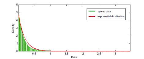
(a)

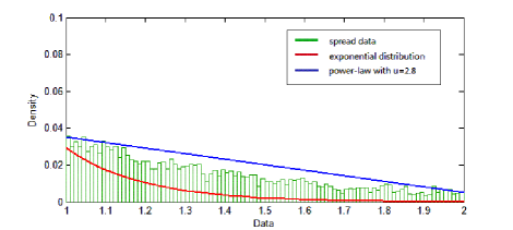
(b)

Figure 1: Power-law Decaying Tail of $\bar{s}$

Correlation between Spread and Volatility: We study the relation between the spread and the volatility of the mid-price return per trade as in Wyart et al. [19]. In their paper, the volatility of the mid-price return per trade is computed from empirical data as $\sigma_{1}=\sqrt{\sum_{i=1}^{N}(m_{i}-m_{i-1})^{2}/N}$, where $N$ is the number of trades that has been observed and $m_{i}$ is the mid-price per trade. They find a strong linear relationship between $\sigma_{1}$ and the mean spread in stationary distribution $E[\bar{s}(\infty)]$. Our model also capture the linear relationship between the volatility of the mid-price return and the spread per trade. To see this, we first simulate $(\bar{s}(\cdot),\bar{m}(\cdot))$ according to (8). Since $(\bar{s}(\cdot),\bar{m}(\cdot))$ is the limit of the price and spread per trade when the arrival rate of trades $\to\infty$, we estimate the volatility $\sigma_{1}$ (up to some constance) of the mid-price return per trade by

$$\hat{\sigma}_{1}^{2}=\lim_{n\to\infty}\frac{1}{n}\sum_{k=1}^{n}(\bar{m}(k\Delta t)-\bar{m}((k-1)\Delta t))^{2}/\Delta t,$$

and we choose $\Delta t=0.1$ unit of time. We compute $\hat{\sigma}_{1}$ as the path average of the simulated path of $\bar{m}(\cdot)$. We also compute $E[\bar{s}(\infty)]$ as the path average taking at every $\Delta t=0.1$ unit of time interval.

	$u$	$\xi$	$r$	$\mu$	$\beta$	$\mu\gamma$	$E[\bar{s}(\infty)]$	$\hat{\sigma}_{1}$
1	2.8	0.08	0.25	12	0.25	9	0.1704	0.0822
2	2.8	0.4	0.25	12	0.25	9	0.7934	0.4074
3	2.8	0.8	0.25	12	0.25	9	1.5862	0.8169
3	2.3	0.08	0.25	12	0.25	9	0.1812	0.0885
4	2.3	0.08	0.5	6	0.25	3	0.1696	0.0848
5	2.3	0.08	0.75	4	0.25	1	0.1559	0.0812

Table 4: Estimation of $E[\bar{s}(\infty)]$ and $\hat{\sigma}_{1}$ under different parameters.

The simulation results reported in Table 4 indicate a linear relation between $E[\bar{s}(\infty)]$ and $\hat{\sigma}_{1}$ that is found in Wyart et al. [19]. Heuristically, without the jump part in (8), $\bar{s}(\cdot)$ becomes a one dimensional reflected Brownian motion with drift $\xi\beta$ and variance coefficient $\xi^{2}r\mu/3$, and the mid-price is simply a Brownian motion with variance coefficient $\xi^{2}r\mu/3$. It is known that the stationary distribution of a reflected Brownian motion is exponential and one can compute that $\hat{\sigma}_{1}=\xi r\mu/(6\beta)$. Also, in the case of no jumps, we can clearly evaluate $\hat{\sigma}_{1}=\xi\sqrt{r\mu/3}$. Therefore, the mean spread and the mean volatility have a linear relationship of the form $E[\bar{s}(\infty)]=l\times\hat{\sigma}_{1}$ with $l=\sqrt{r\mu}/(2\beta\sqrt{3})$. In Table 4, we choose different sets of parameters such that $\sqrt{r\mu}/(2\beta\sqrt{3})\equiv 2$ and one can check that the estimated mean $E[\bar{s}(\infty)]\approx 2\hat{\sigma}_{1}$, so the effect of the jumps is actually relatively minor on the parameter ranges that we explored, for this particular performance measure.

Volatility Clustering: The jump-diffusion limit (8) also captures the volatility clustering feature in limit order book data as reported in a series of empirical studies (see Section G.2 in Gould et al. [9]). To see this, we measure the volatility in the mid-price process as the standard deviation of the mid-price return per 0.1 unit of time over every 10 units long time window. In detail, we compute a time series $\bar{\sigma}(t)$ from the simulated mid-price process $\bar{m}$ as

$$\bar{\sigma}(t)=\sqrt{\frac{1}{99}\sum_{i=1}^{100}(\bar{m}(10t+0.1i)-\frac{1}{100}\sum_{j=1}^{100}\bar{m}(10t+0.1j))^{2}}.$$

To illustrate volatility clustering, in Figure 2, we compare the original time series of the volatility we have computed and its random permutation. In the original time series, peaks are gathering together while in the permuted time series, peaks are uniformly distributed along the time.

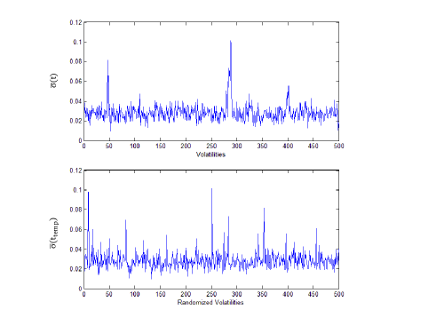
Figure 2: Volatility clustering of realized mid-price returns in simulation data

6 Appendix: Technical Proofs

In this section we provide all of the technical proofs in the order in which the results have been presented.

6.1 The Proof of Theorem 1

Proof of Theorem 1.

In this proof, we will follow the notations as used in Kurtz [13]. Define $X_{n}(\cdot)=(\bar{a}_{n}(\cdot),\bar{b}_{n}(\cdot))\in\mathbb{Z}^{2}$. Define $Y_{n}(\cdot)=(Y_{n}^{i}(\cdot):i\in\mathbb{Z})\in\mathbb{Z}^{\infty}$, where $Y_{n}^{i}(t)$ equals the number of limit sell orders (or minus the number of limit buy orders) on price tick $i$ in the $n$-th LOB system at time $t$. We denote by $E_{1}$ and $E_{2}$ respectively the space of $\mathbb{Z}^{2}$ and $\mathbb{Z}^{\infty}$ that are endowed with the discrete topology. Then, $\{(X_{n}(\cdot),Y_{n}(\cdot))\}$ is a sequence of stochastic processes living in the product space $E_{1}\times E_{2}$.

Note that for each $n$, $(X_{n}(\cdot),Y_{n}(\cdot))$ is a continuous time Markov Chain with countable number of states. Let $\{\mathfrak{F}_{t}^{n}\}$ be the natural filtration associated with $(X_{n}(\cdot),Y_{n}(\cdot))$. Then, one can check that for any $f\in C(E_{1})$,

$$f(X_{n}(t))-\int_{0}^{t}2\mu(f(a(Y_{n}(s)),b(Y_{n}(s)))-f(X_{n}(s)))ds\triangleq f(X_{n}(t))-\int_{0}^{t}\mathcal{A}f(X_{n}(s),Y_{n}(s))ds$$

is a martingale with respect to $\{\mathfrak{F}_{t}^{n}\}$. Here the functional $a:\mathbb{R}^{\infty}\rightarrow\mathbb{R}$ is just the ask price of the LOB at time $s$, more precisely,

$$a(Y_{n}(s))=\min\{i:Y_{n}^{i}(s)>0\}.$$

The functional $b(\cdot)$ can be defined in a similar way. One can also check that for any $g\in C(E_{2})$,

$$g(Y_{n}(t))-\int_{0}^{t}\sum_{i}\xi_{n}\left[\lambda p(i;X_{n}(s))\left(g(Y_{n}(s)+e_{\bar{a}_{n}(s)+i})+g(Y_{n}(s)+e_{\bar{b}_{n}(s)-i})-2g(Y_{n}(s))\right)\right.$$

$$+ \left.\alpha(i;X_{n}(s))\left(Y_{n}^{\bar{a}_{n}(s)+i}(s)(g(Y_{n}(s)-e_{\bar{a}_{n}(s)+i})-g(Y_{n}(s)))+Y_{n}^{\bar{b}_{n}(s)-i}(s)(g(Y_{n}(s)-e_{\bar{b}_{n}(s)-i})-g(Y_{n}(s)))\right)\right]ds$$

$$\triangleq ~{}g(Y_{n}(t))-\int_{0}^{t}\xi_{n}\mathcal{B}g(X_{n}(s),Y_{n}(s))ds$$

is also a martingale. Due to the regularity condition imposed (2), $\{X_{n}(\cdot)\}$ is tight. Therefore, each subsequence of $\{X_{n}(\cdot)\}$ admit a sub-subsequence that converges weakly to some sub-limit process $X(\cdot)$. Then according to Theorem 2.1 and the subsequent Example 2.4 in Kurtz [13], each sub-limit process $X(\cdot)=(\hat{a}(\cdot),\hat{b}(\cdot))$ is a solution to the martingale problem

$$f(X(t))-\int_{0}^{t}\int_{E_{2}}\mathcal{A}f(X(s),y)\pi_{X(s)}(dy)ds,$$ (9)

in the sense that the stochastic process defined by (9) is a martingale. Moreover, in the expression (9), $\pi_{X(s)}(\cdot)$ is the unique stationary distribution of a stochastic process $Y\in E_{2}$ which satisfies the martingale problem

$$g(Y(t))-\int_{0}^{t}\mathcal{B}g(x,Y(u))du.$$

In our case, $\pi_{x}(\cdot)$ is simply the stationary distribution of the LOB system under the parameters $\{p(i;x),\alpha(i;x)\}$.

Now we compute that in (9),

$$\int_{E_{2}}\mathcal{A}f(X(s),y)\pi_{X(s)}(dy)$$

$$= \sum_{i,j}\mu(f(\hat{a}(\cdot)+i,\hat{b}(\cdot)+j)-f(\hat{a}(\cdot),\hat{b}(\cdot)))\pi_{X(s)}(\{a(y)-\hat{a}_{n}(s)=i,b(y)-\hat{b}_{n}(s)=-j\})$$

$$= \sum_{i,j}\mu(f(\hat{a}(\cdot)+i,\hat{b}(\cdot)+j)-f(\hat{a}(\cdot),\hat{b}(\cdot)))[\theta(i;\hat{a}(t),\hat{b}(t))-\theta(i+1;\hat{a}(s),\hat{b}(s))]$$

$$\times[\theta(j;\hat{a}(s),\hat{b}(s))-\theta(j+1;\hat{a}(s),\hat{b}(s))].$$

One can check that the martingale problem (9) has a unique solution $X(\cdot)$, see for instance Chapter 4.4 in Ethier and Kurtz [8]. In particular, $X(\cdot)=(\hat{a}(\cdot),\hat{b}(\cdot))$ is equivalent in distribution to a jump process with jump intensity $2\mu$ and jump size distribution

$$P\left(\hat{a}(t)-\hat{a}(t-)=i,\hat{b}(t)-\hat{b}(t-)=j|\hat{a}(t-),\hat{b}(t-)\right)$$

$$=~{} [\theta(i;\hat{a}(t-),\hat{b}(t-))-\theta(i+1;\hat{a}(t-),\hat{b}(t-))]\times[\theta(j;\hat{a}(t-),\hat{b}(t-))-\theta(j+1;\hat{a}(t-),\hat{b}(t-))].$$

Since $\{X_{n}(\cdot)\}$ is tight and each of its convergent subsequence admits the same limit $X(\cdot)$, we can conclude that $\{X_{n}(\cdot)\}$ weakly converges to $X(\cdot)$. ∎

6.2 The Proof of Theorem 2

Now let us describe the roadmap for the proof of Theorem 2. We first construct some auxiliary process $(\tilde{S}^{n}(\cdot),\tilde{M}^{n}(\cdot))$ living in the same probability space as the underlying process $(\bar{s}^{n}(\cdot),\bar{m}^{n}(\cdot))$. The auxiliary process is a convenient Markov process whose generator can be analyzed to conclude weak convergence to the postulated limiting jump diffusion (8). The auxiliary process has the same dynamics as the target process except when it is on the boundary-layer set $[0,2/\sqrt{n}]\times\mathbb{R}$. We also show the time spent by the two processes on the boundary-layer is small and as a result their difference caused by their different dynamics on the boundary is also small. Actually, such difference is negligible as $n\rightarrow\infty$ and therefore the target process converges to the same limit process.

First, we define the auxiliary process coupled with the target process in a path by path fashion. Recall that by Assumption 6 and (7), we can write

$$\begin{cases}\bar{s}^{n}(t_{k+1})&=\bar{s}^{n}(t_{k})+\Delta_{a}^{n}(\bar{s}^{n}(t_{k}))\vee([-\bar{s}^{n}(t_{k})/2\delta]\delta)+\Delta_{b}^{n}(\bar{s}^{n}(t_{k}))\vee([-\bar{s}^{n}(t_{k})/2\delta]\delta),\\ \bar{m}^{n}(t_{k+1})&=\bar{m}^{n}(t_{k})+\Delta_{a}^{n}((\bar{s}^{n}(t_{k})))\vee([-\bar{s}^{n}(t_{k})/2\delta]\delta)-\Delta_{b}^{n}(\bar{s}^{n}(t_{k}))\vee([-\bar{s}^{n}(t_{k})/2\delta]\delta).\end{cases}$$

Now we define the auxiliary process $(\tilde{S}^{n}(\cdot),\tilde{M}^{n}(\cdot))$ coupled with $(\bar{s}^{n}(\cdot),\bar{m}^{n}(\cdot))$) as

$$\begin{cases}\tilde{S}^{n}(t_{k+1})&=\tilde{S}^{n}(t_{k})+(\Delta_{a}^{n}(\tilde{S}^{n}(t_{k}))+\Delta_{b}^{n}(\tilde{S}^{n}(t_{k})))\vee(-\tilde{S}^{n}(t_{k})),\\ \tilde{M}^{n}(t_{k+1})&=\tilde{M}^{n}(t_{k})+\Delta_{a}^{n}((\tilde{S}^{n}(t_{k})))-\Delta_{b}^{n}(\tilde{S}^{n}(t_{k})),\end{cases}$$ (10)

with the initial condition $\tilde{S}^{n}(0)=\bar{s}^{n}(0)$ and $\tilde{M}^{n}(0)=\bar{m}^{n}(0)$.

Then the main result in this section Theorem 2 is an immediate corollary of the following two propositions.

Proposition 2.

The auxiliary process $(\tilde{S}^{n}(\cdot),\tilde{M}^{n}(\cdot))$ converges weakly to the limit process given by (8).

Proposition 3.

The difference process $\left(\bar{s}^{n}(\cdot)-\tilde{S}^{n}(\cdot),\bar{m}^{n}(\cdot)-\tilde{M}^{n}(\cdot)\right)$ converges weakly to $(0,0)$ on $D_{\mathbb{R}^{2}}[0,t]$ for any $t<\infty$.

Proof of Proposition 3.

For simplicity, we assume that $\xi=1$, otherwise we can divide $\tilde{S}$, $\tilde{M}$ and $\bar{s}$, $\bar{m}$ by the constant $\xi$. Assume also that $V_{k}^{a}\leq c$ for some $c\geq 1$. The general case can be dealt with using truncation because there are only a Poisson number of jumps that arise in $O\left(1\right)$ time.

Now, let us first give a bound for the difference $\bar{s}^{n}(\cdot)-\tilde{S}^{n}(\cdot)$. For fixed $n$, we define $N(t)=\sum_{\{j:t_{j}\leq t\}}(I_{j}^{a}+I_{j}^{b})$, intuitively $N(t)$ corresponds to the number of jumps of the limiting process from time 0 to time $t$. Now we prove by induction that

$$0\leq\bar{s}^{n}(t_{k})-\tilde{S}^{n}(t_{k})\leq\left((1+c)^{N(t_{k})}-1\right)\cdot\frac{2}{\sqrt{n}}.$$ (11)

At $t_{0}=0$, we have $\tilde{S}^{n}(t_{0})=\bar{s}(t_{0})$. Now suppose the relation (11) holds at time $t_{k-1}$, there are two cases at time $t_{k}$, case 1): $N(t_{k})=N(t_{k-1})$, and case 2): $N(t_{k})>N(t_{k-1})$.

First let us consider the case when $N(t_{k})=N(t_{k-1})$. In this case, we know that $\Delta_{a}^{n}(\bar{s}^{n}(t_{k-1}))=\Delta_{a}^{n}(\tilde{S}(t_{k-1})):=\Delta_{a}^{n}$ is independent of $\bar{s}^{n}(t_{k-1})$ and $\tilde{S}^{n}(t_{k-1})$. Also, keep in mind that $\left|\Delta_{a}^{n}\left(t_{k}\right)\right|\leq 1/\sqrt{n}$.  Now we can write the increment of the difference process

$$(\bar{s}^{n}(t_{k})-\tilde{S}^{n}(t_{k}))-(\bar{s}^{n}(t_{k-1})-\tilde{S}^{n}(t_{k-1}))$$

$$=~{} \Delta_{a}^{n}\vee([-\bar{s}^{n}(t_{k})/(2\delta)]\delta)+\Delta_{b}^{n}\vee([-\bar{s}^{n}(t_{k})/(2\delta)]\delta)-(\Delta_{a}^{n}+\Delta_{b}^{n})\vee(-\tilde{S}^{n}(t_{k-1})).$$ (12)

Therefore, if $\bar{s}^{n}(t_{k-1})\geq\tilde{S}^{n}(t_{k-1})\geq 2/\sqrt{n}$, we have

$$(\bar{s}^{n}(t_{k})-\tilde{S}^{n}(t_{k}))-(\bar{s}^{n}(t_{k-1})-\tilde{S}^{n}(t_{k-1}))=\Delta_{a}^{n}+\Delta_{b}^{n}-(\Delta_{a}^{n}+\Delta_{b}^{n})=0$$

and as a result $\bar{s}^{n}(t_{k-1})-\tilde{S}^{n}(t_{k-1})=\bar{s}^{n}(t_{k})-\tilde{S}^{n}(t_{k})$. If $\bar{s}^{n}(t_{k-1})\geq 2/\sqrt{n}\geq\tilde{S}^{n}(t_{k-1})\geq 0$, We have

$$(\bar{s}^{n}(t_{k})-\tilde{S}^{n}(t_{k}))-(\bar{s}^{n}(t_{k-1})-\tilde{S}^{n}(t_{k-1}))$$

$$=~{} \Delta_{a}^{n}+\Delta_{b}^{n}-(\Delta_{a}^{n}+\Delta_{b}^{n})\vee(-\tilde{S}^{n}(t_{k-1}))=-(\tilde{S}^{n}(t_{k-1})+\Delta_{a}^{n}+\Delta_{b}^{n})^{-}\leq 0.$$

Therefore,

$$\bar{s}^{n}(t_{k-1})-\tilde{S}^{n}(t_{k-1})\geq\bar{s}^{n}(t_{k})-\tilde{S}^{n}(t_{k})\geq\frac{2}{\sqrt{n}}-(\tilde{S}^{n}(t_{k-1})+\Delta_{a}^{n}+\Delta_{b}^{n})\geq 0.$$

Otherwise, we have $0\leq\tilde{S}^{n}(t_{k-1})\leq\bar{s}^{n}(t_{k-1})\leq 2/\sqrt{n}$. In this case, one can check that for any fixed $\tilde{S}^{n}(t_{k})=\tilde{s}$ and $\bar{s}^{n}(t_{k})=s$, the increment of the difference process (12) reaches its maximum at $\Delta_{a}^{n}=-1//\sqrt{n}$ and $\Delta_{b}^{n}=-\tilde{s}+/\sqrt{n}$ and its minimum at $\Delta_{a}^{n}=\Delta_{b}^{n}=-[s/2\delta]\delta$. Hence,

$$\tilde{s}-s\leq\left(\bar{s}^{n}(t_{k})-\tilde{S}^{n}(t_{k})\right)-\left(\bar{s}^{n}(t_{k-1})-\tilde{S}^{n}(t_{k-1})\right)\leq 0\vee(\frac{1}{\sqrt{n}}-\frac{s}{2}-\tilde{s}).$$

Plugging in $\tilde{S}^{n}(t_{k})=\tilde{s}$ and $\bar{s}^{n}(t_{k})=s$, we have

$$0\leq\bar{s}^{n}(t_{k})-\tilde{S}^{n}(t_{k})\leq(s-\tilde{s})\vee(\frac{1}{\sqrt{n}}+\frac{s}{2})\leq(\bar{s}^{n}(t_{k-1})-\tilde{S}^{n}(t_{k-1}))\vee\frac{2}{\sqrt{n}}.$$

The last inequality holds as $s=\bar{s}^{n}(t_{k-1})\leq 2/\sqrt{n}$. In summary, we have proved that when $N(t_{k})=N(t_{k-1})$, if the relation (11) holds at time $t_{k-1}$, so does it at time $t_{k}$.

Now if $N(t_{k})\geq N(t_{k-1})+1$, intuitively, at least one jump occurs in $\Delta_{a}^{n}$ and $\Delta_{b}^{n}$. If $I_{k}^{a}=1$ we have

$$\Delta_{a}^{n}(\tilde{S}^{n}(t_{k-1}))=I_{k}^{a}V_{k}^{a}[\tilde{S}^{n}(t_{k-1})/(2\delta)]\delta,\text{ and }\Delta_{a}^{n}(\bar{s}^{n}(t_{k-1}))=I_{k}^{a}V_{k}^{a}[\bar{s}^{n}(t_{k-1})/(2\delta)]\delta.$$

If in addition $I_{k}^{b}=1$, then

$$\Delta_{b}^{n}(\tilde{S}^{n}(t_{k-1}))=I_{k}^{b}V_{k}^{b}[\tilde{S}^{n}(t_{k-1})/(2\delta)]\delta,\text{ and }\Delta_{b}^{n}(\bar{s}^{n}(t_{k-1}))=I_{k}^{b}V_{k}^{b}[\bar{s}^{n}(t_{k-1})/(2\delta)]\delta,$$

and therefore,

$$\bar{s}^{n}(t_{k})-\tilde{S}^{n}(t_{k})\leq(\bar{s}^{n}(t_{k-1})-\tilde{S}^{n}(t_{k-1}))(I_{k}^{a}V_{k}^{a}+I_{k}^{b}V_{k}^{b}+1)/2.$$

As

$$0\leq V_{k}^{a}+V_{k}^{b}+1\leq 2c+1\text{ \ and \ }0\leq\bar{s}^{n}(t_{k-1})-\tilde{S}^{n}(t_{k-1})\leq((c+1)^{N(t_{k-1})}-1)\cdot\frac{2}{\sqrt{n}},$$

by the induction assumption we have

$$0\leq\bar{s}^{n}(t_{k})-\tilde{S}^{n}(t_{k})\leq((c+1)^{N(t_{k-1})}-1)(2c+1)\cdot\frac{2}{\sqrt{n}}\leq((c+1)^{N(t_{k})}-1)\cdot\frac{2}{\sqrt{n}}.$$

If $I_{k}^{b}=0$, then following a similar argument as in the case when $N(t_{k})=N(t_{k-1})$, we have

$$\bar{s}^{n}(t_{k})-\tilde{S}^{n}(t_{k}) \leq(\bar{s}^{n}(t_{k-1})-\tilde{S}^{n}(t_{k-1}))(V_{k}^{a}+1)+(\bar{s}^{n}(t_{k-1})-\tilde{S}^{n}(t_{k-1}))\vee\frac{2}{\sqrt{n}}$$

$$=((c+1)^{N(t_{k})}-1)\cdot\frac{2}{\sqrt{n}}\text{ ~{}~{} as }c\geq 1.$$

In summary, we have proved the relation (11) of $\tilde{S}^{n}(\cdot)$ and $\bar{s}^{n}(\cdot)$ by induction.

Now let us turn to the difference $\bar{m}^{n}(\cdot)-\tilde{M}^{n}(\cdot)$. Actually, $\bar{m}^{n}(t)-\tilde{M}^{n}(t)$ can be decomposed into two parts,

$$\bar{m}^{n}(t)-\tilde{M}^{n}(t)$$

$$\leq~{} \sum_{0\leq k\leq[nt]:N(t_{k+1})=N(t_{k})}\left[\Delta_{a}^{n}(t_{k})\vee([\bar{s}^{n}(t_{k-1})/(2\delta)]\delta)-\Delta_{b}^{n}(t_{k})\vee([\bar{s}^{n}(t_{k-1})/(2\delta)]\delta)-(\Delta_{a}^{n}(t_{k})-\Delta_{b}^{n}(t_{k}))\right]$$

$$~{}+\sum_{i=1}^{N(t)}([\bar{s}^{n}(t_{k-1})/(2\delta)]\delta-[\tilde{S}^{n}(t_{k-1})/(2\delta)]\delta)(I_{k_{i}}^{a}V_{k_{i}}^{a}+I_{k_{i}}^{b}V_{k_{i}}^{b}),$$

where $\{t_{k_{i}}\}$ are the jump times. We denote the two summation parts as

$$\bar{m}^{n}(t)-\tilde{M}^{n}(t)=\epsilon_{0}^{n}(t)+\epsilon_{1}^{n}(t).$$

Intuitively, $\epsilon_{0}^{n}(t)$ is the error corresponding to the diffusion part when $I^{a}_{k}=I^{b}_{k}=0$ and $\epsilon_{1}^{n}(t)$ is the error corresponding to the jumps. In the summation part $\epsilon_{0}^{n}(t)$, we write $\Delta_{a}^{n}(\bar{s}^{n}(t_{k}))=\Delta_{a}^{n}(\tilde{S}^{n}(t_{k}))=\Delta_{a}^{n}(t_{k})$ , because they are independent of $\bar{s}^{n}(t_{k})$ and $\tilde{S}^{n}(t_{k})$ when when $I^{a}_{k}=I^{b}_{k}=0$.

Following a same induction argument as for $\bar{s}^{n}-\tilde{S}^{n}$, we can show that the error caused by jumps $\epsilon_{1}^{n}(t)$ satisfies that

$$\epsilon_{1}^{n}(t)\leq((1+2c)^{N(t)}-1)\cdot\frac{2}{\sqrt{n}}.$$

On the other hand, note that $\epsilon_{0}^{n}(t)$ equals

$$\sum_{0\leq k\leq[nt]:N(t_{k+1})=N(t_{k})}\left[\Delta_{a}^{n}(t_{k})\vee([\bar{s}^{n}(t_{k-1})/(2\delta)]\delta)-\Delta_{b}^{n}(t_{k})\vee([\bar{s}^{n}(t_{k-1})/(2\delta)]\delta)-(\Delta_{a}^{n}(t_{k})-\Delta_{b}^{n}(t_{k}))\right]$$

$$= \sum_{0\leq k\leq[nt]:N(t_{k+1})=N(t_{k})}\left[\left(\Delta_{a}^{n}(t_{k})\vee([\bar{s}^{n}(t_{k-1})/(2\delta)]\delta)-\Delta_{a}^{n}(t_{k})\right)-\left(\Delta_{b}^{n}(t_{k})\vee([\bar{s}^{n}(t_{k-1})/(2\delta)]\delta)-\Delta_{b}^{n}(t_{k})\right)\right].$$

Since $\Delta_{a}^{n}(t_{k})$ and $\Delta_{b}^{n}(t_{k})$ are independent and identically distributed, we have that for any $k\geq 1$

$$E[\epsilon_{0}^{n}(t_{k})-\epsilon_{0}^{n}(t_{k-1})|\mathcal{F}_{t_{k}}^{n}]=~{} P(N(t_{k})=N(t_{k-1}))\cdot\left(E\left[\Delta_{a}^{n}(t_{k})\vee([\bar{s}^{n}(t_{k-1})/(2\delta)]\delta)-\Delta_{a}^{n}(t_{k})\right]\right.$$

$$\left.-E\left[\Delta_{b}^{n}(t_{k})\vee([\bar{s}^{n}(t_{k-1})/(2\delta)]\delta)-\Delta_{b}^{n}(t_{k})\right]\right)=0,$$

where $\mathcal{F}_{t_{k}}^{n}$ is the $\sigma$-field generated by $\{\Delta_{a}^{n}(t_{i}),\Delta_{b}^{n}(t_{i}),\tilde{S}^{n}(t_{i})\}_{i=1}^{k}$. Therefore, the process $\epsilon_{0}^{n}(\cdot)$ is a martingale under the filtration $\mathcal{F}^{n}$. Besides, as $|\Delta_{a}^{n}(t_{k})|\leq 1/\sqrt{n}$ when $N(t_{k})=N(t_{k-1})$, we have

$$|\epsilon_{0}^{n}(t_{k})-\epsilon_{0}^{n}(t_{k-1})|\leq\frac{2}{\sqrt{n}}~{}I(\bar{s}^{n}(t_{k-1})<\frac{2}{\sqrt{n}}).$$

The quadratic variation

$$[\epsilon_{0}^{n}](t)~{}\leq\frac{4}{n}\sum_{i=0}^{[nt]}I(\bar{s}^{n}(t_{i})<\frac{2}{\sqrt{n}}).$$

Recall that we have proved $\bar{s}^{n}(\cdot)\geq\tilde{S}^{n}(\cdot)$,

$$[\epsilon_{0}^{n}](t)~{}\leq\frac{4}{n}\sum_{i=0}^{[nt]}I(\tilde{S}^{n}(t_{i})<\frac{2}{\sqrt{n}}).$$

Since $2/\sqrt{n}\rightarrow 0$, for any $\zeta>0$ we have

$$\lim_{n\rightarrow\infty}[\epsilon_{0}^{n}](t)~{}\leq\lim_{n\rightarrow\infty}4\int_{0}^{t}I(\tilde{S}^{n}(u)<\zeta)du\leq\lim_{n\rightarrow\infty}4\int_{0}^{t}f^{\zeta}(\tilde{S}^{n}(u))du,$$

where $f^{\zeta}(\cdot)$ is a smooth function on $\mathbb{R}^{+}$ and satisfies $f(x)=1$ for all $0\leq x\leq\zeta$, $0\leq f(x)\leq 1$ for $\zeta\leq x\leq 2\zeta$ and $f(x)=0$ for $x>2\zeta$. (Such function can be constructed, for instance, by convolution.) Since $f^{\zeta}(\cdot)$ is bounded and $\tilde{S}^{n}(\cdot)$ converges weakly to the limit process (8), we have

$$\lim_{n\rightarrow\infty}E[[\epsilon_{0}^{n}](t)]~{}\leq\lim_{n\rightarrow\infty}4E[\int_{0}^{t}f^{\zeta}(\tilde{S}^{n}(u))du]=4E[\int_{0}^{t}f^{\zeta}(\bar{s}(u))du]\leq 4E[\int_{0}^{t}I(\bar{s}(u)\leq 2\zeta)],$$

As the limit process $\bar{s}(\cdot)$ has the same dynamics as a reflected Brownian motion except when at the finite time of jumps on $[0,t]$, we have $E[\int_{0}^{t}I(\bar{s}(u)\leq 2\zeta)]\rightarrow 0$ as $\zeta\rightarrow 0$. Since $\zeta$ can be arbitrarily small, we conclude that the expected quadratic variation $E[[\epsilon_{0}^{n}](t)]\rightarrow 0$ as $n\rightarrow 0$ for any $t<\infty$. By Doob’s Inequality, we have that for all fixed $\zeta>0$,

$$P(\max_{0\leq u\leq t}|\epsilon_{0}^{n}(u)|>\zeta)\leq\frac{E[[\epsilon_{0}^{n}](t)]}{\zeta^{2}}\rightarrow 0.$$

Therefore, $\epsilon_{0}^{n}(\cdot)$ converges weakly to $x(\cdot)\equiv 0$ in space $D[0,t]$ for all $t<\infty$.

In the end, it is given in Assumption 3 that $nP(I_{k}^{a}V_{k}^{a}+I_{k}^{b}V_{k}^{b}\neq 0)=2\gamma+o(1)$, so the counting process $N(\cdot)$ converges to a Poisson process with rate $2\mu\gamma$. Therefore, for any $t<\infty$

$$E[\max_{0\leq u\leq t}|((2c+1)^{N(u)}-1)\frac{2}{\sqrt{n}}|]=E[((2c+1)^{N(t)}-1)\frac{2}{\sqrt{n}}]=O(\frac{1}{\sqrt{n}}).$$

As a result, the process $((2c+1)^{N(\cdot)}-1)\frac{2}{\sqrt{n}}$ converges weakly to $x(\cdot)\equiv 0$ in space $D[0,t]$. Recall that we have proved that $((2c+1)^{N(\cdot)}-1)\frac{2}{\sqrt{n}}$ is an upper bound of $|\bar{s}^{n}(\cdot)-\tilde{S}^{n}(\cdot)|$ and the ‘jump part’ of $|\bar{m}^{n}(\cdot)-\tilde{M}^{n}(\cdot)|$. As a consequence, we can conclude that the difference process $(\bar{s}^{n}(\cdot)-\tilde{S}^{n}(\cdot),\bar{m}^{n}(\cdot)-\tilde{M}^{n}(\cdot))$ converges weakly to $(0,0)$ on any compact interval $[0,t]$. ∎

Proof of Proposition 2.

Define $N_{a}(t)=\sum_{\{j:t_{j}\leq t\}}I_{j}^{a}$, $N_{b}(t)=\sum_{\{j:t_{j}\leq t\}}I_{j}^{b}$, and note that $N_{a}\left(\cdot\right)$, $N_{b}\left(\cdot\right)$ are two independent Poisson processes with rate $\gamma\mu$ each. Next, define $\tilde{S}^{n}(0)=\bar{s}^{n}(0)\geq 0$, and $\tilde{M}^{n}(0)=\bar{m}^{n}(0),$ and set

$$S_{a}^{n}\left(t\right)=\sum_{\{j:t_{j}\leq t\}}(-1)^{R_{j}^{a}}[U_{j}^{a}/(\sqrt{n}\delta_{n})]\delta_{n},\text{ \ }S_{b}^{n}\left(t\right)=\sum_{\{j:t_{j}\leq t\}}(-1)^{R_{k}^{b}}[U_{k}^{b}/(\sqrt{n}\delta_{n})]\delta_{n}).$$

We will also define

$$S^{n}\left(t\right) = S_{a}^{n}\left(t\right)+S_{b}^{n}\left(t\right)+\bar{s}^{n}(0),$$

$$M^{n}\left(t\right) = S_{a}^{n}\left(t\right)-S_{b}^{n}\left(t\right)+\bar{m}^{n}(0),$$

(so by convention we set $t_{0}=0$ and $S^{n}\left(0\right)=\bar{s}^{n}(0)$). Also, we define

$$R_{1}^{n}(t)=S^{n}\left(t\right)-\min(S^{n}\left(u\right):u\leq t,0).$$

Let $A=\inf\{t\geq 0:N_{a}\left(t\right)\geq 1\}$ and $B=\inf\{t\geq 0:N_{b}\left(t\right)\geq 1\}$ be the first arrival times of $N_{a}\left(\cdot\right)$ and $N_{b}\left(\cdot\right)$, respectively. Since

$$\tilde{S}^{n}(t_{k})=(\Delta_{a}^{n}(\tilde{S}^{n}(t_{k}))+\Delta_{b}^{n}(\tilde{S}^{n}(t_{k}))+\tilde{S}^{n}(t_{k}))^{+},$$

we have that on $\min(A,B)>t$

$$\tilde{S}^{n}(t)=R^{n}\left(t\right).$$

The strategy proceeds as follows.

Step 1): Show that if $\left(\bar{s}^{n}(0),\bar{m}^{n}(0)\right)\Rightarrow\left(\bar{s}(0),\bar{m}(0)\right)$, the processes $(S_{a}^{n}\left(t\right),S_{b}^{n}\left(t\right):t\geq 0)$ converges weakly in $D[0,\infty)$ to the process $\left(X\left(t\right):t\geq 0\right)$ defined via

$$X_{1}\left(t\right) = \bar{s}(0)-\eta t+W_{a}\left(t\right)+W_{b}\left(t\right),$$

$$X_{2}\left(t\right) = \bar{m}(0)+W_{a}\left(t\right)-W_{b}\left(t\right).$$

Step 2): Once Step 1) has been executed we can directly apply the continuous mapping principle to conclude joint weak convergence on $[0,\min(A,B))$ of the processes

$$R^{n}(\cdot) \Rightarrow R\left(\cdot\right):=X_{1}\left(\cdot\right)-\min\left(X_{1}\left(u\right):0\leq u\leq\cdot\right),$$

$$M^{n}(\cdot) \Rightarrow X_{2}\left(\cdot\right).$$

Step 3): By invoking the Skorokhod embedding theorem, we can assume that the joint weak convergence in Step 2) occurs almost surely. We can add the jump right at time $\min\left(A,B\right)$ without changing the distribution of $X_{1}\left(t\right)$ and $\tilde{S}^{n}(t)$ for $t<\min\left(A,B\right)$. More precisely, define

$$D=I\left(A<B\right)R\left(A\right)V^{a}/2+I\left(B\leq A\right)R\left(B\right)V^{b}/2,$$

where $V^{b}$ and $V^{a}$ are i.i.d. copies of $V_{k}^{b}$ and $V_{k}^{a}$ respectively, and we also define

$$D^{n}=I\left(A<B\right)[R^{n}\left(A\right)V^{a}/(2\delta)]\delta+I\left(B\leq A\right)[R^{n}\left(B\right)V^{b}/(2\delta)]\delta.$$

Then put on $t\in[0,\min\left(A,B\right)]$

$$\tilde{S}^{n}(t) = R^{n}\left(t\right)I\left(t<\min\left(A,B\right)\right)+I\left(t=\min\left(A,B\right)\right)(R^{n}\left(\min\left(A,B\right)\right)+D^{n}),$$

$$\bar{s}(t) = R\left(t\right)I\left(t<\min\left(A,B\right)\right)+I\left(t=\min\left(A,B\right)\right)(R\left(\min\left(A,B\right)\right)+D),$$

$$\tilde{M}^{n}(t) = M^{n}(t)I\left(t<\min\left(A,B\right)\right)$$

$$+I\left(t=\min\left(A,B\right)\right)I\left(A<B\right)[R^{n}\left(A\right)V^{a}/(2\delta)]\delta$$

$$-I\left(t=\min\left(A,B\right)\right)I\left(B\leq A\right)[R^{n}\left(B\right)V^{b}/(2\delta)]\delta,$$

$$\bar{m}(t) = X_{2}(t)I\left(t<\min\left(A,B\right)\right)$$

$$+I\left(t=\min\left(A,B\right)\right)I\left(A<B\right)R\left(A\right)V^{a}/2$$

$$-I\left(t=\min\left(A,B\right)\right)I\left(B\leq A\right)R\left(B\right)V^{b}/2\delta.$$

So, assuming Step 2) and using Skorokhod embedding we then conclude that

$$\sup_{0\leq t\leq\min\left(A,B\right)}\left|\tilde{S}^{n}(t)-\bar{s}(t)\right|+\sup_{0\leq t\leq\min\left(A,B\right)}\left|\tilde{M}^{n}(t)-\bar{m}(t)\right|\rightarrow 0$$

almost surely.

Step 4): Finally, note that the convergence extends throughout the interval $[0,t]$ by repeatedly applying Steps 1) to 3) given that there are only finitely many jumps in $[0,t]$. Clearly then this procedure completes the construction to the solution of the SDE (8).

So, we see that everything rests on the execution of Step 1), and for this we invoke the martingale central limit theorem (see Ethier and Kurtz [8], Theorem 7.1.4). Define

$$Z_{k}^{a}\left(n\right)=(-1)^{R_{k}^{a}}[U_{k}^{a}/(\sqrt{n}\delta_{n})]\delta_{n},\text{ \ \ \ }Z_{k}^{b}\left(n\right)=(-1)^{R_{k}^{b}}[U_{k}^{b}/(\sqrt{n}\delta_{n})]\delta_{n}.$$

We have that

$$EZ_{k}^{a}\left(n\right) = E([U_{k}^{a}/(\sqrt{n}\delta_{n})]\delta_{n})(-\beta/(\sqrt{n}))=\beta EZ_{k}^{b}\left(n\right)=\begin{cases}\frac{-\beta E\left(U_{1}^{a}\right)}{n}+o(1/n)&\text{ if }\delta_{n}=o(1/\sqrt{n}),\\ \frac{-\beta E\left(\left[U_{1}^{a}\right]\right)}{n}+o\left(1/n\right)&\text{ if }\delta_{n}=1/\sqrt{n},\end{cases}$$

and

$$Var\left(Z_{k}^{a}\left(n\right)\right) = E([U_{k}^{a}/(\sqrt{n}\delta_{n})]^{2}\delta_{n}^{2})-\left(EZ_{k}^{a}\left(n\right)\right)^{2}=E([U_{k}^{a}/(\sqrt{n}\delta_{n})]^{2}\delta_{n}^{2})-O\left(1/n\right).$$

We write

$$S_{a}^{n}\left(t\right)=M_{a}^{n}\left(t\right)+\mu tEZ_{k}^{b}\left(n\right)=M_{a}^{n}(t)-\eta t+o(1),$$

where $M_{a}^{n}\left(t\right)$ is a martingale, and we have that

$$\sup_{0\leq t\leq T}|M_{n}^{a}\left(t\right)-M_{n}^{a}\left(t_{-}\right)|\leq(\theta/\sqrt{n}+\delta_{n}),$$

therefore

$$E\sup_{0\leq t\leq T}|M_{n}^{a}\left(t\right)-M_{n}^{a}\left(t_{-}\right)|\text{ }+E\sup_{0\leq t\leq T}|M_{n}^{a}\left(t\right)-M_{n}^{a}\left(t_{-}\right)|^{2}=o\left(1\right)$$

as $n\rightarrow\infty$, which verifies conditions a) and b.1) from Ethier and Kurtz [8],Theorem 7.1.4. Moreover, we have that

$$\left[M_{a}^{n},M_{a}^{n}\right]\left(t\right)=\sum_{j=1}^{N\left(nt\right)}[U_{j}^{a}/(\sqrt{n}\delta_{n})]^{2}\delta_{n}^{2}\rightarrow t\sigma=\left\{\begin{array}[]{cl}t\mu E(\left[U_{j}^{a}\right]^{2})&\text{if }\delta_{n}=1/\sqrt{n},\\ t\mu E(\left(U_{j}^{a}\right)^{2})&\text{if }\delta_{n}=o(1/\sqrt{n}).\end{array}\right.$$

Furthermore, we have that

$$E\max_{t\leq T}\left|\left[M_{a}^{n},M_{a}^{n}\right]\left(t\right)-\left[M_{a}^{n},M_{a}^{n}\right]\left(t_{-}\right)\right|\leq(\theta/\sqrt{n}+\delta_{n})^{2}=o\left(1\right),$$

which corresponds to condition b.2) in Ethier and Kurtz [8],Theorem 7.1.4. Hence, we conclude that

$$M_{a}^{n}\left(\cdot\right)\Rightarrow W_{a}\left(\cdot\right)$$

under the uniform topology on compact sets. A completely analogous strategy is applicable to conclude $M_{a}^{n}\left(\cdot\right)\Rightarrow W_{b}\left(\cdot\right)$. The convergence holds jointly due to independence and therefore we obtain the conclusion required in Step 1). As indicated earlier, Steps 2) to 4) now follow directly. ∎

References

• Billingsley [1999] P. Billingsley. Convergence of Probability Measures, 2nd Edition. Wiley, 1999.
• Bouchard et al. [2002] J. Bouchard, M. Mezard, and M. Potters. Statistical properties of stock order books: empirical results and models. Quantitative Finance, 2(4):251, 2002.
• Bouchard et al. [2004] J. Bouchard, Y. Gefen, M. Potters, and M. Wyart. Fluctuations and response in financial markets: the subtle nature of ‘random’ price changes. Quantitative Finance, 4(2):176, 2004.
• Cartea et al. [2011] A. Cartea, S. Jaimungal, and J. Ricci. Buy low sell high: a high frequency trading perspective. Working paper, 2011.
• Cont and Larrard [2013] R. Cont and A. Larrard. Price dynamics in a Markovian limit order book market. SIAM Journal on Financial Mathematics, 4(1):1–25, 2013.
• Cont et al. [2010] R. Cont, S. Stoikov, and R. Talreja. A stochastic model for order book dynamics. Operations Research, 58:549–563, 2010.
• Cont et al. [2013] R. Cont, A. Kukanov, and S. Stoikov. The price impact of order book events. Journal fo Financial Econometrics, 2013.
• Ethier and Kurtz [1986] S. Ethier and T. Kurtz. Markov Processes: Characterization and Convergence. Wiley, 1986.
• Gould et al. [2012] M. Gould, M. Porter, S. Wiliams, M. McDonald, D. Fenn, and S. Howison. Limit order book. Working paper, 2012. URL http://arxiv.org/abs/1012.0349.
• Hasbrouck and Saar [2009] J. Hasbrouck and G. Saar. Technology and liquidity provision: The blurring of traditional definitions. Journal of Finanical Markets, 12:143–172, 2009.
• Hautsch and Huang [2012] N. Hautsch and R. Huang. The market impact of a limit order. Journal of Economic Dynamics and Control, 36:501–522, 2012.
• Horst and Paulsen [2013] U. Horst and M. Paulsen. A law of large numbers for limit order books. Working paper, 2013.
• Kurtz [1992] T. G. Kurtz. Averaging for martingale problems and stochastic approximation. In Ioannis Karatzas and Daniel Ocone, editors, Applied Stochastic Analysis, volume 177 of Lecture Notes in Control and Information Sciences, pages 186–209. Springer Berlin Heidelberg, 1992.
• Lakner et al. [2013] P. Lakner, J. Reed, and S. Stoikov. High frequency asymptotic for the limit order book. Working paper, 2013.
• Maglaras et al. [2012] C. Maglaras, C.C. Moallemi, and H. Zheng. Optimal order routing in a fragmented market. Working paper, 2012.
• Muni Toke [2010] I. Muni Toke. Econophysics of Order-Driven Markets, chapter “Market making” in an order book model and its impact on the bid-ask spread. Springer-Verlag Milan, 2010.
• Potters and Bouchard [2003] M. Potters and J. Bouchard. More statistical properties of order books and price impact. Physica A, 324(1-2):133, 2003.
• Sowers et al. [2013] R. Sowers, A. Kirilenko, and X. Meng. A multiscale model of high-frequencey trading. Algorithmic Finance, 2(1):59–98, 2013.
• Wyart et al. [2008] M. Wyart, J. Bouchard, J. Kockelkoren, M. Potters, and M. Vettorazzo. Relation between bid-ask spread, impact and volatility in order-driven markets. Quantitative Finance, 8(1):41, 2008.
• Zheng et al. [2013] B. Zheng, F. Roueff, and F. Abergel. Modelling Bid and Ask prices using constrained Hawkes processes ergodicity and scaling limit. Working paper, 2013.
• Zovko and Farmer [2002] I. Zovko and J. Farmer. The power of patience: a behavioral regularity in limit order placement. Quantitative Finance, 2(5):387, 2002.