The period function
and the harmonic balance method

Abstract.

In this paper we consider several families of potential non-isochronous systems and study their associated period functions. Firstly, we prove some properties of these functions, like their local behavior near the critical point or infinity, or their global monotonicity. Secondly, we show that these properties are also present when we approach to the same questions using the Harmonic Balance Method.

1. Introduction and main results

Given a planar differential system having a continuum of periodic orbits, its period function is defined as the function that associates to each periodic orbit its period. To determine the global behavior of this period function is an interesting problem in the qualitative theory of differential equations either as a theoretical question or due to its appearance in many situations. For instance, the period function is present in mathematical models in physics or ecology, see [14, 33, 36] and the references therein; in the study of some bifurcations [10, pp. 369-370]; or to know the number of solutions of some associated boundary value problems, see [7, 8].

In particular, there are several works giving criteria for determining the monotonicity of the period function associated with some systems, see [7, 16, 19, 34, 38] and the references therein. Results about non monotonous period functions have also recently appeared, see for instance [18, 21, 25].

The so-called $N$-th order Harmonic Balance Method (HBM) consists on approximating the periodic solutions of a non-linear differential equation by using truncated Fourier series of order $N$. It is mainly applied with practical purposes, although in many cases there is no a theoretical justification. In most of the applications this method is used to approach isolated periodic solutions, see for instance [17, 23, 31, 30, 29, 28]. Since the HBM also provides an approximation of the angular frequency of the searched periodic solution, it can be also used to get its period.

Hence, applying the HBM to systems of differential equations having a continuum of periodic orbits we can obtain approximations of the corresponding period functions. The main goal of this paper is to illustrate this last assertion trough the study of several concrete planar systems. This approach is also used for instance in [3, 4, 32]. A main difference among these works and our paper is that we also carry out a detailed analytic study of the involved period functions.

More specifically, in this work we will consider several families of planar potential systems, $\ddot{x}=f(x),$ having continua of periodic orbits. We will study analytically their corresponding period functions and we will see that the approximations of the period functions obtained using the $N$-th order HBM, for $N=1$, keep the essential properties of the actual period functions: local behavior near the critical point and infinity, monotonicity, oscillations,… For the case of the Duffing oscillator we also consider $N=2$ and $3$. In particular, the method that we introduce using resultants gives an analytic way to deal with the 3rd order HBM, answering question (iv) in [32, p. 180].

First, we focus in the following two families of potential differential systems:

$$\left\{\begin{array}[]{l}\dot{x}=-y,\\ \dot{y}=x+x^{2m-1},\qquad m\in\mathbb{N}\quad{\rm and}\quad m\geq 2,\end{array}\right.$$ (1)

and

$$\left\{\begin{array}[]{lll}\dot{x}=y,\\ \dot{y}=-\frac{x}{(x^{2}+k^{2})^{m}},\qquad k\in\mathbb{R}\setminus\{0\},\,\,m\in[1,\infty).\end{array}\right.$$ (2)

Each system of these families has a continuum of periodic orbits around the origin. Thus, we can talk about its periodic function $T$ which associates to each periodic orbits passing trough $(x,y)=(A,0)$ its period $T(A)$. In addition, we will denote by $T_{N}(A)$ the approximation to $T(A)$ by using $N$-th order HBM; see Section 2.2 for the precise definition of $T_{N}(A)$.

System (1) is an extension of the Duffing-harmonic oscillator which corresponds to the case $m=2$. The case $m=2$ has been studied by many authors, see [23, 24, 27, 30]. The exact period function of this particular system is given as an elliptic function and so it is easier to obtain analytic properties of $T$. Our analytic study is valid for all integers $m\geq 2.$

System (2) with $m=1$ and by taking the limit $k\rightarrow 0$ is equivalent to the second order differential equation $x\ddot{x}+1=0$, which is studied in [31] as a model of plasma physics. Thus, system (2) can be seen as an extension of the singular second order differential equation $x\ddot{x}+1=0$. In a forthcoming paper we explore the relationship between the periodic solutions of (2) with $m=1$ and their corresponding periods with the solutions of the limiting case $x\ddot{x}+1=0.$

We have chosen these two families due to their simplicity and because, as we will see, their corresponding period functions are monotonous, being the first one decreasing and the second one increasing.

For the first family (1), in addition to the monotonicity of $T$, we perform a more detailed study of some properties of $T$. More precisely, we give the behavior of $T$ near to the origin and at infinity and we compare them with the results obtained by the HBM.

Theorem 1.1.

System (1) has a global center at the origin and its period function $T$ is decreasing. Moreover, at $A=0$,

$$T(A)=2\pi\left(1-\frac{(2m-1)!!}{(2m)!!}\,A^{2m-2}+{S}(m)\,A^{4m-4}+O(A^{6m-6})\right),$$ (3)

where ${S}(m)=\frac{(2m-1)(4m-1)!!}{m(4m)!!}-\frac{(m-1)(2m-1)!!}{m(2m)!!}$; and

$$T(A)\sim B\left(\frac{1}{2m},\frac{1}{2}\right)\frac{2}{\sqrt{m}\,A^{m-1}},\quad A\to\infty,$$ (4)

where $B(\cdot,\cdot)$ is the Beta function.

Proposition 1.2.

By applying the first-order HBM to system (1) we get the decreasing function

$$T_{1}(A)=\frac{2^{m}\pi}{\sqrt{\frac{(2m-1)!}{(m-1)!m!}A^{2m-2}+2^{2m-2}}}.$$ (5)

Moreover, at $A=0$,

$$T_{1}(A)=2\pi\left(1-\frac{(2m-1)!!}{(2m)!!}A^{2m-2}+\frac{3}{2}\left(\frac{(2m-1)!!}{(2m)!!}\right)^{2}A^{4m-4}+O(A^{6m-6})\right),$$

and

$$T_{1}(A)\sim\frac{2^{m}\pi}{\sqrt{\frac{(2m-1)!}{(m-1)!m!}}\,A^{m-1}},\quad A\to\infty.$$ (6)

By Theorem 1.1, we know that the period function $T$ of system (1) is decreasing. Proposition 1.2 asserts that this property is already present in its first order approximation obtained with the HBM. Additionally, we can see that the first and second terms of the Taylor series at $A=0$ of $T(A)$ and $T_{1}(A)$ coincide, while the third one is different. Furthermore, from (4) and (6) it follows that $T(A)$ and $T_{1}(A)$ have similar behaviors at infinity.

In the case of the Duffing-harmonic oscillator ($m=2$ in (1)) we will apply the $N$-th order HBM, $N=2,3,$ for computing the approximations $T_{N}(A)$ of the period function $T(A)$, see Section 5. We prove that $T(A)-T_{N}(A)=O(A^{2N+4})$ at $A=0.$ We believe that similar results hold for (1) with $m>2$, nevertheless, for the sake of shortness, do not study this question it this paper. We also will see that the approximations $T_{N}(A),N=1,2,3,$ at infinity become sharper by increasing $N$.

For the family (2) we have similar results. We only will deal with the global behaviors of $T$ and $T_{1}$ skipping the study of these functions near zero and infinity.

Theorem 1.3.

System (2) has a center at the origin and its period function $T$ is increasing. Moreover, the center is global for $m=1$ and non-global otherwise.

Proposition 1.4.

By applying the first-order HBM to system (2) we obtain the increasing function

$$T_{1}(A)=2\pi\sqrt{\sum_{j=0}^{m}\left(\frac{1}{2}\right)^{2j}{m\choose j}{{2j+1}\choose j}k^{2(m-j)}A^{2j}}.$$ (7)

Note that again, as in system (1), with the first-order HBM we obtain that $T_{1}(A)$ and $T(A)$ have the same monotonicity behavior.

In Section 6 we consider the family of polynomial potential systems

$$\left\{\begin{array}[]{l}\dot{x}=-y,\\ \dot{y}=x+k\,x^{3}+x^{5},\quad k\in\mathbb{R},\end{array}\right.$$ (8)

which for some values of $k$ has a global center. In [25, Thm. 1.1 (b)] it is proved that the period function associated to the global center at the origin has at most one oscillation. Joining this result with a similar study that the one made for system (1) at the origin and at infinity, that we will omit for the sake of shortness, we obtain:

Theorem 1.5.

Consider system (8) with $k\in(-2,\infty)$. Let $T$ be the period function associated to the origin, which is a global center. Then:

• The function $T$ is monotonous decreasing for $k\geq 0$.

• The function $T$ starts increasing, until a maximum (a critical period) and then decreases towards zero, for $k\in(-2,0)$.

• At the origin

  $$T(A)=2\pi-\frac{3}{4}k\pi A^{2}+\frac{57k^{2}-80}{128}\pi A^{4}+O(A^{6}),$$

  and at infinity

  $$T(A)\sim\frac{2{B}(\frac{1}{6},\frac{1}{2})}{\sqrt{3}}\frac{1}{A^{2}}\approx\frac{8.4131}{A^{2}}.$$

We prove:

Proposition 1.6.

By applying the first-order HBM to the family (8) we get:

$$T_{1}(A)=\frac{8\pi}{\sqrt{16+12kA^{2}+10A^{4}}}.$$

In particular,

• The function $T_{1}(A)$ is decreasing for $k\geq 0$.

• The function $T_{1}(A)$ starts increasing, has a maximum and then decreases towards zero, for $k\in(-2,0)$.

• At the origin

  $$T_{1}(A)=2\pi-\frac{3}{4}k\pi A^{2}+\frac{54k^{2}-80}{128}\pi A^{4}+O(A^{6}),$$

  and at infinity

  $$T_{1}(A)\sim\frac{4\pi\sqrt{10}}{5}\frac{1}{A^{2}}\approx\frac{7.9477}{A^{2}}.$$

Once more, we can see that the function $T_{1}(A)$ obtained by applying the first order HBM captures and reproduces quite well the actual behavior of $T(A).$

Remark 1.7.

In fact, the shape of the function $T_{1}(A)$ for $k\in(-2,0)$ does not vary until $k=-2\sqrt{10}/3\approx-2.107$. For $k\leq-2\sqrt{10}/3$, it is no more defined for all $A\in\mathbb{R}.$ Somehow, this phenomenon reflects the fact that for $k\leq-2$ the center in not global. Notice, that for $k<-2$, system (8) has three centers.

Motivated by all our results, in Section 7 we study the relationship between the Taylor series of $T(A)$ and $T_{N}(A)$ with $N=1,2$ at $A=0$ for an arbitrary smooth potential.

When the system has a center and its period function is constant, then the center is called isochronous. The problem about the existence and characterization of isochronous center has also been extensively studied, see [11, 12, 13, 22, 26]. To end this introduction we want to comment that we have not succeeded in applying the HBM to detect isochronous potentials. We have unfold in 1-parameter families one of the simplest potential isochronous systems, the one given by a rational potential function, see [14]. Our attempts to use the low order HBM to detect the value of the parameter that corresponds to the isochronous case have not succeed.

The paper is organized as follows. In Section 2 we give some preliminary results which include a known result for studying the monotonicity of the period function. Also we describe the $N$-th order HBM. In Section 3 we prove our analytical results about the monotonicity of the period function of systems (1) and (2) and their local behavior at the center and at infinity, see Theorems 1.1 and 1.3. In Section 4 we prove Propositions 1.2 and 1.4, both dealing with the HBM. In Section 5 we focus on the study of the Duffing-harmonic oscillator and we also apply the 2-th order and 3-rd order HBM. Section 6 deals with the family of planar polynomial potential systems having a non-monotonous period function. Finally, Section 7 studies the local behavior near zero of $T(A)$ and $T_{N}(A)$ with $N=1,2$, of an arbitrary smooth potential system.

2. Preliminary results

This section is divided in two parts. The first one is devoted to recall some definitions, as well as, to give the framework for the study of the period function of (1) and (2) from an analytical point of view. In the second one we will give the description of the $N$-order Harmonic Balance Method, which we will apply in our second analysis of the period function.

2.1. Definitions and some analytical tools

The systems studied in this paper are all potential systems,

$$\left\{\begin{array}[]{lll}\dot{x}=-y,\\ \dot{y}=\,F^{\prime}(x),\end{array}\right.$$ (9)

with associated Hamiltonian function $H(x,y)=y^{2}/2+F(x)$, where $F:\Omega\subset\mathbb{R}\to\mathbb{R}$ is a real smooth function, $F(0)=0$ and $0\in\Omega,$ an open real interval.

Let $p_{0}$ be a singular point of (9). It is said that $p_{0}$ is a center if there exists an open neighborhood $U$ of $p_{0}$ such that each solution $\gamma(t)$ of (9) with $\gamma(0)\in U-\{p_{0}\}$ defines a periodic orbit $\gamma$ surrounding $p_{0}$. The largest neighborhood $\mathcal{P}$ with this property is called the period annulus of $p_{0}$. If $\Omega=\mathbb{R}$ and $\mathcal{P}=\mathbb{R}^{2}$, then $p_{0}$ is called a global center.

The following result characterizes systems (9) having global centers.

Lemma 2.1.

If $F(x)$ has a minimum at $0$, then system (9) has a center at the origin. Moreover, the center is global if and only if $F^{\prime}(x)\neq 0$ for all $x\neq 0$ and $F(x)$ tends to infinity when $|x|$ does.

Suppose that (9) has a center with period annulus $\mathcal{P}$. For each periodic orbit $\gamma\in\mathcal{P}$ we define $T(\gamma)$ to be the period of $\gamma$. Thus, the map

$$T:\mathcal{P}\rightarrow\mathbb{R}_{+},\qquad\gamma\mapsto T(\gamma),$$

is called the period function associated with $\mathcal{P}$. It is said that the map $T$ is monotone increasing (respectively monotone decreasing) if for each couple of periodic orbits $\gamma_{0}$ and $\gamma_{1}$ in $\mathcal{P}$, with $\gamma_{0}$ in the interior of bounded region surrounded by $\gamma_{1}$, it holds that $T(\gamma_{1})-T(\gamma_{0})>0$ (respectively $<0$). When $T$ is constant, then the center is called isochronous center.

If we fix a transversal section $\Sigma$ to $\mathcal{P}$ and we take a parametrization $\sigma(A)$ of $\Sigma$ with $A\in(0,A^{*})\subset\mathbb{R}_{+}$, then we can denote by $\gamma_{A}$ the periodic orbit passing through $\sigma(A)$ and by $T(A)$ its period. That is, we have the map $T:(0,A^{*})\rightarrow\mathbb{R}_{+}$, $A\mapsto T(A)$. When $T$ is not monotonous then either it is constant or it has local maxima or minima. The isolated zeros of $T^{\prime}(A)$ are called critical periods. It is not difficult to prove that the number of critical periods does not depend neither of $\Sigma$ nor of its parametrization.

Next, we will recall two results about some properties of the period function $T$ which we will apply in our study of the families (1), (2) and (8). The first result is an adapted version to system (9), of statement 3 of [16, Prop. 10] and gives a criterion about the monotonicity of $T$. The second one is an adapted version of [12, Thm. C], which will allow us to describe the behavior of $T$ at infinity.

Proposition 2.2.

Suppose that system (9) has a center at the origin. Let $T$ be the period function associated to the period annulus of the center. Then

• If $F^{\prime}(x)^{2}-2F(x)F^{\prime\prime}(x)\geq 0$ (not identically $0$) on $\Omega$, then $T$ is increasing.

• If $F^{\prime}(x)^{2}-2F(x)F^{\prime\prime}(x)\leq 0$ (not identically $0$) on $\Omega$, then $T$ is decreasing.

To state the second result, we need some previous constructions and definitions.

Let $\gamma_{h}(t)=(x_{h}(t),y_{h}(t))$ be a periodic orbit of (9) contained in $\mathcal{P}$ corresponding to the level set $\{H=h\}$. This orbit crosses the axis $y=0$ at the points determined by $F(x_{h}(t))=h$. Since $F$ has a minimum at $x=0$, near the origin the above equation has two solutions, one of them on $x>0$ which will be denoted by $F_{+}^{-1}(h)$ and the other one on $x<0$ which will be denoted by $F_{-}^{-1}(h)$. We note that this property remains for all $h\in(0,h^{*}):=H(\mathcal{P})\setminus\{0\}$. For each $h>0$ we define the function

$$l_{F}(h)=F_{+}^{-1}(h)-F_{-}^{-1}(h)$$ (10)

which gives the length of the projection to the $x$-axis of $\gamma_{h}$. See Figure 1.

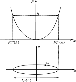
Figure 1. Definition of $l_{F}$ for system (9).

Definition 2.3.

Given two real numbers $a$ and $M$, it is said that a continuous function $g(x)$ has $Mx^{a}$ as dominant term of its asymptotic expansion at $x=x_{0}\in\mathbb{R}\cup\{\infty\}$ if

$$\lim_{x\to x_{0}}\frac{g(x)-Mx^{a}}{x^{a}}=0.$$

This property is denoted by $g(x)\sim Mx^{a}$ at $x=x_{0}$.

Theorem 2.4.

Assume that (9) has a global center at the origin. Let $l_{F}(h)$ be as in (10) and suppose that $l^{\prime}_{F}(h)\sim Mh^{a},$ at $h=\infty$ with $a>-1$ and $M>0$. Then, the period function of (9) satisfies $T(h)\sim Ch^{a+1/2}$ at $h=\infty$, where $C=\sqrt{2}MB(a+1,3/2)$, and $B(\cdot,\cdot)$ is the Beta function.

Next lemma computes the function $l_{F}(h)$ for system (1).

Lemma 2.5.

The function $l_{F}(h)$ associated to (1) satisfies that $\textit{l}_{F}(h)\sim 2(2mh)^{\frac{1}{2m}}$ at $h=\infty$.

Proof.

We start studying the algebraic curve $\mathcal{C}:=\{p(x,h)=F(x)-h=0\}$ at infinity. For that, we consider the homogenization

$$P(X,H,Z)=X^{2m}+mX^{2}Z^{2m-2}-2mHZ^{2m-1},$$ (11)

of $p(x,h)$ in the real projective plane $\mathbb{RP}^{2}$. From (11) it follows that $[0:1:0]$ is the unique point at infinity of $\mathcal{C}$, and $\mathcal{C}$ in the chart that contains such point is given by the set of zeros of the polynomial

$$\tilde{p}(\tilde{x},\tilde{z}):=P(\tilde{x},1,\tilde{z})=\tilde{x}^{2m}+m\tilde{x}^{2}z^{2m-2}-2m\tilde{z}^{2m-1}.$$

For studying $\mathcal{C}$ at infinity we will obtain a parametrization of it close to the point $[0:1:0]$. As usual, we will use the Newton polygon associated to $\tilde{p}$. The $\it{carrier}$ of $\tilde{p}$ is ${\rm carr}(\tilde{p})=\{(2m,0),(2,2m-2),(0,2m-1)\}$, whence the Newton polygon is the straight line joining $(2m,0)$ and $(0,2m-1)$ whose equation is

$$\tilde{z}=-\left(\frac{2m-1}{2m}\right)\tilde{x}+2m-1.$$

In $\tilde{p}(\tilde{x},\tilde{z})$ we replace $\tilde{z}=z_{0}t^{2m}$ and $\tilde{x}=x_{0}t^{2m-1}$, then

$$\tilde{p}(x_{0}t^{2m-1},z_{0}t^{2m})=mx_{0}^{2}z_{0}^{2(m-1)}t^{2(2m^{2}-1)}+(x_{0}^{2m}-2mz_{0}^{2m-1})t^{2m(2m-1)}.$$

For $x_{0}$ fixed we consider

$$\begin{array}[]{lll}\phi(z_{0},t)&=&(x_{0}^{2m}-2mz_{0}^{2m-1})t^{2m(2m-1)}+mx_{0}^{2}z_{0}^{2(m-1)}t^{2(2m^{2}-1)}\\ &=&t^{2m(2m-1)}\tilde{\phi}(z_{0},t),\end{array}$$

where $\tilde{\phi}(z_{0},t)=x_{0}^{2m}-2mz_{0}^{2m-1}+mx_{0}^{2}z_{0}^{2(m-1)}t^{2(m-1)}$. It is clear that $\tilde{\phi}(z_{0}^{\ast},0)=0$ for $z_{0}^{\ast}$ solution of $x_{0}^{2m}-2mz_{0}^{2m-1}=0$. Moreover

$$\frac{\partial\tilde{\phi}}{\partial z_{0}}(z_{0}^{\ast},0)=-2m(2m-1)(z_{0}^{\ast})^{2(m-1)}\neq 0.$$

From the implicit function theorem there exists a function $z_{0}(t):(\mathbb{R},0)\rightarrow\mathbb{R}$ such that $z_{0}(0)=z_{0}^{\ast}$ and $\phi(z_{0}(t),t)=0$ for $t\in(\mathbb{R},0).$ Since $\phi(z_{0}(t),t)$ is an analytic function, $z_{0}(t)$ also is it. Hence we can write $z_{0}(t)=c_{0}+c_{1}t+c_{2}t^{2}+\ldots$, moreover as $z_{0}(0)=z_{0}^{\ast}$ then

$$z_{0}(t)=z_{0}^{\ast}+O(t).$$

From $x_{0}^{2m}-2mz_{0}^{2m-1}=0$ and the above equation it follows that

$$x_{0}(t)=\pm((2m)^{\frac{1}{2m}}(z_{0}^{\ast})^{\frac{2m-1}{2m}}+O(t^{\frac{2m-1}{2m}})).$$

Then the parametrization of $\mathcal{C}$ is $t\mapsto(\tilde{x}(t),\tilde{z}(t))$ where

$$\tilde{x}(t) =t^{2m-1}x_{0}(t)=(2m)^{\frac{1}{2m}}(z_{0}^{\ast})^{\frac{2m-1}{2m}}t^{2m-1}+O(t^{\frac{4m^{2}-1}{2m}})$$ (12)

$$\tilde{z}(t) =t^{2m}z_{0}(t)=z_{0}^{\ast}t^{2m}+O(t^{2m+1}).$$ (13)

Recall that the relation between $(\tilde{x},\tilde{z})$ and $(x,h)$ is given by $\tilde{x}=x/h$ and $\tilde{z}=1/h$. From (13) it follows that $1/h\sim z_{0}^{\ast}t^{2m}$ at $h=\infty$. Using this behavior and (12) we get $x\sim\pm(2mh)^{\frac{1}{2m}}$ at $h=\infty$. Hence $F_{\pm}^{-1}(h)\sim(2mh)^{\frac{1}{2m}}$ and from (10) it follows that $\textit{l}_{F}(h)\sim 2(2mh)^{\frac{1}{2m}}$. ∎

2.2. The Harmonic Balance Method

In this section we recall the $N$-th order HBM adapted to our setting. Consider the second order differential equation

$$\ddot{x}=f(x,\alpha),\quad\alpha\in\mathbb{R}.$$

Suppose that it has a $T$-periodic solution $x(t)$ such that $x(0)=A$ and $\dot{x}(0)=0.$ This $T$-periodic function $x(t)$ satisfies the functional equation

$$\mathcal{F}:=\mathcal{F}(x(t),\ddot{x}(t),\alpha)=\ddot{x}(t)-f(x(t),\alpha)=0.$$

On the other hand, $x(t)$ has the Fourier series:

$$x(t)=\frac{\tilde{a}_{0}}{2}+\sum_{k=1}^{\infty}\left(\tilde{a}_{k}\cos(k\omega t)+\tilde{b}_{k}\sin(k\omega t)\right),$$

where $\omega:=2\pi/T$ is the angular frequency of $x(t)$ and the coefficients $\tilde{a}_{k}$ and $\tilde{b}_{k}$ are the so-called Fourier coefficients, which are defined as

$$\tilde{a}_{k}=\frac{2}{T}\int_{0}^{T}x(t)\cos(k\omega t)\,dt\quad\mbox{and}\quad\tilde{b}_{k}=\frac{2}{T}\int_{0}^{T}x(t)\sin(k\omega t)\,dt\quad\mbox{for $k\geq 0$}.$$

(Although we not write explicitly, $\tilde{a}_{k}$, $\tilde{b}_{k}$, and $\omega$ depend on $\alpha$ and $A$, that is, $\tilde{a}_{k}:=\tilde{a}_{k}(\alpha,A)$, $\tilde{b}_{k}:=\tilde{b}_{k}(\alpha,A)$, and $\omega:=\omega(\alpha,A)$.) Hence it is natural to try to approximate the periodic solutions of the functional equation $\mathcal{F}=0$ by using truncated Fourier series of order $N$, i.e. trigonometric polynomials of degree $N$.

The $N$-th order HBM consists of the following four steps.

1. Consider a trigonometric polynomial

$$x_{{}_{N}}(t)=\frac{a_{0}}{2}+\sum_{k=1}^{N}\left(a_{k}\cos(k\omega_{N}t)+b_{k}\sin(k\omega_{N}t)\right).$$ (14)

2. Compute the $T$-periodic function $\mathcal{F}_{N}:=\mathcal{F}(x_{{}_{N}}(t),\ddot{x}_{{}_{N}}(t))$, which has also an associated Fourier series, that is,

$$\mathcal{F}_{N}=\frac{\mathcal{A}_{0}}{2}+\sum_{k=1}^{\infty}\left(\mathcal{A}_{k}\cos(k\omega_{N}t)+\mathcal{B}_{k}\sin(k\omega_{N}t)\right),$$

where $\mathcal{A}_{k}=\mathcal{A}_{k}({\mathbf{a}},{\bf b},\omega)$ and $\mathcal{B}_{k}=\mathcal{B}_{k}({\mathbf{a}},{\bf b},\omega)$, $k\geq 0,$ with ${\mathbf{a}}=(a_{0},a_{1},\ldots,a_{{}_{N}})$ and ${\bf b}=(b_{1},\ldots,b_{{}_{N}})$.

3. Find values ${\bf a}$, ${\bf b}$, and $\omega$ such that

$$\mathcal{A}_{k}({\bf a},{\bf b},\omega)=0\quad\mbox{and}\quad\mathcal{B}_{k}({\bf a},{\bf b},\omega)=0\quad\mbox{for}\quad 0\leq k\leq N.$$ (15)

4. Then the expression (14), with the values of ${\bf a}$, ${\bf b}$, and $\omega$ obtained in point 3, provides candidates to be approximations of the actual periodic solutions of the initial differential equation. In particular the values $2\pi/\omega$ give approximations of the periods of the corresponding periodic orbits.

We end this short explanation about HBM with several comments:

(a) The above set of equations (15) is a system of polynomial equations which usually is very difficult to solve. For this reason in many works, see for instance [31, 32] and the references therein, only small values of $N$ are considered. We also remark that in general the coefficients of $x_{{}_{N}}(t)$ and $x_{{}_{N+1}}(t)$ do not coincide at all. Hence, going from order $N$ to order $N+1$ in the method, implies to compute again all the coefficients of the Fourier polynomial.

(b) The equations $\mathcal{A}_{k}({\bf a},{\bf b},\omega)=0$ and $\mathcal{B}_{k}({\bf a},{\bf b},\omega)=0$ for $0\leq k\leq N$ are equivalent to

$$\frac{2}{T}\int_{0}^{T}\mathcal{F}_{N}\cos(k\omega t)\,dt=0\quad\mbox{and}\quad\frac{2}{T}\int_{0}^{T}\mathcal{F}_{N}\sin(k\omega t)\,dt=0\quad\mbox{for}\quad 0\leq k\leq N.$$

(c) The linear combination, $a_{k}\cos(k\omega t)+b_{k}\sin(k\omega t)$, of the harmonics of order $k$, with $k=0,1,\ldots N$, can be expressed as

$$a_{k}\cos(k\omega t)+b_{k}\sin(k\omega t)=\frac{\bar{c}_{k}\,e^{ik\omega t}+c_{k}\,e^{-ik\omega t}}{2},$$

where $c_{k}=a_{k}+ib_{k}$, and $\bar{c}_{k}$ is the complex conjugated of $c_{k}$. Therefore, we can use the HBM with the last notation, because the truncated Fourier series can be written as

$$x_{N}(t)=\sum_{k=1}^{N}\frac{\bar{c}_{k}\,e^{ik\omega_{N}t}+c_{k}\,e^{-ik\omega_{N}t}}{2},\quad k=1,\ldots,N.$$ (16)

(d) In general, although in many concrete applications HBM seems to give quite accurate results, it is not proved that the found Fourier polynomials are approximations of the actual periodic solutions of differential equation. Some attempts to prove this relationship can be seen in [17] and the references therein.

3. The period function from the analytical point of view

In this section we prove our main results concerning the period function of systems (1) and (2). For proving Theorem 1.1 we will apply Lemma 2.1 and Proposition 2.2 to determine the existence of a global center of (1) and the monotonicity of its period function. To find the Taylor series of $T$ at the origin we will use an old idea, due to Cherkas([6]), which consists in transforming (1) into an Abel equation. Finally, in the last part of the proof, that corresponds to the behavior at infinity of $T$, we will use Theorem 2.4 and Lemma 2.5. Theorem 1.3 follows using similar tools.

3.1. Proof of Theorem 1.1

System (1) is of the form (9) with $F(x)=x^{2}/2+x^{2m}/2m$. Clearly, by Lemma 2.1, the origin $(0,0)$ is a global center. Moreover, the set $\{(A,0)\in\mathbb{R}^{2}\,|\,A>0\}$ is a transversal section to $\mathcal{P}$. Thus, $T$ can be expressed as function depending on the parameter $A$.

Some easy computations give that

$$\begin{array}[]{l}F^{\prime}(x)^{2}-2F(x)F^{\prime\prime}(x)=-(\frac{m-1}{m})((2m-1)+x^{2m-2})x^{2m}\leq 0.\end{array}$$

Therefore, Proposition 2.2.$(ii)$ implies that the period function $T(A)$ associated to $\mathcal{P}$ is decreasing for all $m$.

For obtaining the Taylor series of $T$ at $A=0$ we will consider system (1) in polar coordinates and initial condition $(A,0)$, that is,

$$\left\{\begin{array}[]{l}\dot{R}=\sin(\theta)\cos^{2m-1}(\theta)R^{2m-1}\\ \dot{\theta}=1+\cos^{2m}(\theta)R^{2m-2},\end{array}\right.\quad R(0)=A,\quad\theta(0)=0,$$ (17)

which is equivalent to the differential equation

$$\frac{dR}{d\theta}=\frac{\sin(\theta)\cos^{2m-1}(\theta)R^{2m-1}}{1+\cos^{2m}(\theta)R^{2m-2}},\quad R(0)=A.$$

By applying the Cherkas transformation [6]: $r=r(R;\theta)=\frac{R^{2m-2}}{1+\cos^{2m}(\theta)R^{2m-2}}$ to the previous equation, we obtain the Abel differential equation

$$\frac{dr}{d\theta}=P(\theta)r^{3}+Q(\theta)r^{2},\quad r(A;0)=\frac{A^{2m-2}}{1+A^{2m-2}},$$ (18)

where $P(\theta)=(2-2m)\sin(\theta)\cos^{4m-1}(\theta)$ and $Q(\theta)=2(2m-1)\sin(\theta)\cos^{2m-1}(\theta).$ Near the solution $r=0$, the solutions of this Abel equation can be written as the power series

$$r(A;0)=\frac{A^{2m-2}}{1+A^{2m-2}}+\sum_{i=2}^{\infty}u_{i}(\theta)\left(\frac{A^{2m-2}}{1+A^{2m-2}}\right)^{i}$$ (19)

for some functions $u_{i}(\theta)$ such that $u_{i}(0)=0$ which can be computed solving recursively linear differential equations obtained by replacing (19) in (18). For instance,

$$u_{2}(\theta)=\int_{0}^{\theta}Q(\psi)d\psi\qquad{\rm and}\qquad u_{3}(\theta)=\int_{0}^{\theta}(P(\psi)+2Q(\psi)u_{2}(\psi))d\psi.$$

From the expression of $\dot{\theta}$ in (17) and using variables $(r,\theta)$ again, we obtain

$$\begin{array}[]{rl}\displaystyle T(A)&\displaystyle=\int_{0}^{2\pi}\frac{d\theta}{1+\cos^{2m}(\theta)R^{2m-2}}\displaystyle=\int_{0}^{2\pi}(1-\cos^{2m}(\theta)\,r)d\theta=\\ &\displaystyle=2\pi-\int_{0}^{2\pi}\cos^{2m}(\theta)\left(\frac{A^{2m-2}}{1+A^{2m-2}}+\sum_{i=2}^{\infty}u_{i}(\theta)\left(\frac{A^{2m-2}}{1+A^{2m-2}}\right)^{i}\right)d\theta.\end{array}$$

Then, we have

$$T(A)=2\pi-\sum_{k\geq 1}\mathcal{S}_{k}\left(\frac{A^{2m-2}}{1+A^{2m-2}}\right)^{k},$$

with

$$\mathcal{S}_{1}=\int_{0}^{2\pi}\cos^{2m}(\theta)d\theta\quad{\rm and}\quad\mathcal{S}_{k}=\int_{0}^{2\pi}\cos^{2m}(\theta)u_{k}(\theta)d\theta\quad{\rm for}\quad k\geq 2.$$

It is easy to see that for $|A|<1,$

$$\frac{A^{2m-2}}{1+A^{2m-2}}=A^{2m-2}-A^{4m-4}+O(A^{6m-6}),\,\Big{(}\frac{A^{2m-2}}{1+A^{2m-2}}\Big{)}^{2}=A^{4m-4}+O(A^{6m-6}).$$

Thus,

$$T(A)=2\pi-\mathcal{S}_{1}A^{2m-2}-(\mathcal{S}_{2}-\mathcal{S}_{1})A^{4m-4}-O(A^{6m-6}).$$

Easy computations show that

$$\mathcal{S}_{1}=2\pi\frac{(2m-1)!!}{(2m)!!},\qquad\mathcal{S}_{2}=2\pi\left(\frac{2m-1}{m}\right)\left(\frac{(2m-1)!!}{(2m)!!}-\frac{(4m-1)!!}{(4m)!!}\right),$$

where, given $n\in\mathbb{N}^{+}$, $n!!$ is defined recurrently as $n!!=n\times(n-2)!!$ with 1!!=1 and 2!!=2. Hence, introducing ${S}(m)=\mathcal{S}_{2}-\mathcal{S}_{1}$ we obtain (3), as we wanted to prove.

Finally, for studying the behavior of $T$ at infinity we will apply Theorem 2.4. By Lemma 2.5, we have that at $h=\infty,$ $\textit{l}_{F}(h)\sim 2(2mh)^{\frac{1}{2m}}$. Then

$$\textit{l}^{\,\prime}_{F}(h)\sim\frac{(2m)^{\frac{1}{2m}}}{m}h^{-\frac{2m-1}{2m}}.$$

If we denote by $\widetilde{T}(h)$ the period function of (1) in terms of $h$, then, from Theorem 2.4, it follows that $\widetilde{T}(h)$ at $h=\infty$ satisfies

$$\widetilde{T}(h)\sim B\left(\frac{1}{2m},\frac{1}{2}\right)2^{\frac{m+1}{2m}}m^{-\frac{2m-1}{2m}}h^{-\frac{m-1}{2m}}.$$ (20)

Now, using that $h=A^{2}/2+A^{2m}/2m$, we get

$$h^{-\frac{m-1}{2m}}=\left(\frac{A^{2}}{2}+\frac{A^{2m}}{2m}\right)^{-\frac{m-1}{2m}}=A^{-(m-1)}\left(\frac{1}{2A^{2m-2}}+\frac{1}{2m}\right)^{-\frac{m-1}{2m}}$$

and we have

$$\lim_{A\to\infty}\frac{A^{-(m-1)}\left(\frac{1}{2A^{2m-2}}+\frac{1}{2m}\right)^{-\frac{m-1}{2m}}-(2m)^{\frac{m-1}{2m}}A^{-(m-1)}}{A^{-(m-1)}}=0.$$

Hence $T(A)=\widetilde{T}(A^{2}/2+A^{2m}/2m)$, and from previous equation and (20) we obtain

$$T(A)\sim B\left(\frac{1}{2m},\frac{1}{2}\right)2^{\frac{m+1}{2m}}m^{-\frac{2m-1}{2m}}(2m)^{\frac{m-1}{2m}}A^{-(m-1)},$$

which after a simplification reduces to (4).

3.2. Proof of Theorem 1.3

By using the transformation $u=x/k$, $v=yk^{m-1}$, and the rescaling of time $\tau=-t/k^{m}$, system (2) becomes

$$\left\{\begin{array}[]{lll}\dot{x}=-y,\\ \dot{y}=\displaystyle\frac{x}{(x^{2}+1)^{m}},\qquad m\in[1,\infty),\end{array}\right.$$ (21)

where we have reverted to the original notation $(x,y)$ and $t$.

The associated Hamiltonian function to (21) is $H(x,y)=\frac{y^{2}}{2}+F(x)$ with

$$F(x)=\left\{\begin{array}[]{ll}-\frac{1}{2}\ln(x^{2}+1),&\mbox{if $m=1$,}\\ \\ -\frac{1}{2(m-1)(x^{2}+1)^{m-1}}+\frac{1}{2(m-1)},&\mbox{if $m>1$.}\end{array}\right.$$

It is clear that for all $m$ the function $F$ is smooth at the origin and has a non-degenerate minimum. Thus, from Lemma 2.1, system (21) has a center at the origin with some period annulus $\mathcal{P}$.

From a straightforward computation we get

$$F^{\prime}(x)^{2}-2F(x)F^{\prime\prime}(x)=\left\{\begin{array}[]{ll}\frac{x^{2}+(x^{2}-1)\ln(x^{2}+1)}{(x^{2}+1)^{2}},&\mbox{if $m=1$,}\\ \\ \frac{1-mx^{2}+((2m-1)x^{2}-1)(x^{2}+1)^{m-1}}{(m-1)(x^{2}+1)^{2m}},&\mbox{if $m>1$.}\end{array}\right.$$

To prove that the period function $T$ associated to $\mathcal{P}$ is increasing we will apply Proposition 2.2.($i$). Hence we need only to show that $F^{\prime}(x)^{2}-2F(x)F^{\prime\prime}(x)\geq 0$. For $m=1$ it is clear. For $m>1$ the denominator of $F^{\prime}(x)^{2}-2F(x)F^{\prime\prime}(x)$ is positive, then remains to prove that its numerator is positive.

By taking $w=x^{2}+1$, the numerator of $F^{\prime}(x)^{2}-2F(x)F^{\prime\prime}(x)$ with $m>1$ is $(2m-1)w^{m}-2mw^{m-1}-mw+m+1$ or equivalently,

$$(w-1)^{2}\left((2m-1)w^{m-2}+(2m-2)w^{m-3}+\ldots+m+1\right),$$

which is clearly positive.

To finish the proof, we will discuss about the globality of the center. For $m=1$ the $(0,0)$ is a global minimum of $H$. Thus, (21) and therefore (2) have a global center at the origin. For $m>1$ the level curve

$$\mathcal{C}_{\frac{1}{2m-2}}=\left\{\frac{1}{2(m-1)(x^{2}+1)^{m-1}}-\frac{y^{2}}{2}=0\right\}$$

has two disjoin components. Indeed, it is formed by the graphics of the functions

$$y=\pm\frac{1}{\sqrt{(m-1)(x^{2}+1)^{m-1}}},$$

which are well-defined for all $x\in\mathbb{R}$ because $m>1$. This implies that the center at the origin of (21) is bounded by $\mathcal{C}_{\frac{1}{2m-2}}$ and therefore it is not global. The same happens with (2).

4. The period function from the point of view of HBM

In this section we prove Propositions 1.2 and 1.4.

4.1. Proof of Proposition 1.2

System (1) is equivalent to the second order differential equation $\ddot{x}+x+x^{2m-1}=0$ with initial conditions $x(0)=A$, $\dot{x}(0)=0$. For applying HBM we consider the functional equation

$$\mathcal{F}(x(t),\ddot{x}(t))=\ddot{x}(t)+x(t)+x(t)^{2m-1}=0.$$ (22)

By symmetry, for applying the 1st order HBM we can look for a solution of the form $x(t)=a_{1}\cos(\omega_{1}t)$. We substitute it in (22). By using that

$$\cos^{2m-1}(\omega_{1}t)=\frac{1}{2^{2m-2}}\sum_{k=0}^{m-1}{2m-1\choose k}\cos((2m-2k-1)\omega_{1}t)$$

and reordering terms we have that the vanishing of the coefficient of $\cos(\omega_{1}t)$ in $\mathcal{F}_{1}(x(t),\ddot{x}(t))$ implies

$$2^{2m-2}(\omega_{1}^{2}-1)-\frac{(2m-1)!}{(m-1)!\,m!}a_{1}^{2m-2}=0.$$

From the initial conditions we have $a_{1}=A$, whence

$$\omega_{1}=\frac{1}{2^{m-1}}\sqrt{\frac{(2m-1)!}{(m-1)!m!}A^{2m-2}+2^{2m-2}}.$$

Therefore, the first approximation $T_{1}(A)$ to $T(A)$ of system (1) is

$$T_{1}(A)=\frac{2\pi}{\frac{1}{2^{m-1}}\sqrt{\frac{(2m-1)!}{(m-1)!m!}A^{2m-2}+2^{2m-2}}}.$$ (23)

Easy computations shows that the Taylor series of $T_{1}$ at $A=0$ is

$$T_{1}(A)=2\pi\left(1-\frac{(2m)!}{(m!)^{2}\,2^{2m}}\,A^{2m-2}+\left(\frac{(2m)!}{(m!)^{2}\,2^{2m}}\right)^{2}\,A^{4m-4}+O(A^{6m-6})\right).$$

By using the identities $(2m)!/(2^{m}\,m!)=(2m-1)!!$ and $2^{m}\,m!=(2m)!!$ we have the expression of the statement.

For studying the behavior at infinity we can write $T_{1}(A)$ as

$$T_{1}(A)=2^{m}\pi A^{-m+1}\left(\frac{(2m-1)!}{(m-1)!\,m!}+\frac{2^{2m-2}}{A^{2m-2}}\right)^{-1/2},$$

thus,

$$\lim_{A\to\infty}\frac{2^{m}\pi A^{-m+1}\left(\frac{(2m-1)!}{(m-1)!m!}+\frac{2^{2m-2}}{A^{2m-2}}\right)^{-1/2}-2^{m}\pi A^{-m+1}\left(\frac{(2m-1)!}{(m-1)!m!}\right)^{-1/2}}{A^{-m+1}}=0.$$

Hence $T_{1}(A)$ at infinity satisfies (6).

4.2. Proof of Proposition 1.4

System (2) is equivalent to the second order differential equation

$$(x^{2}+k^{2})^{m}\ddot{x}+x=0,$$ (24)

with initial conditions $x(0)=A$, $\dot{x}(0)=0$. For simplicity in the computations, we consider the complex form, given in (16), of the first-order HBM

$$x_{1}(t)=\frac{1}{2}\left(\bar{c}e^{i\omega_{1}t}+ce^{-i\omega_{1}t}\right),$$ (25)

where $c=a+bi$. By using the binomial expression

$$(x^{2}+k^{2})^{m}=\sum_{j=0}^{m}{m\choose j}x^{2j}k^{2(m-j)},$$

and by replacing (25) in (24), after some computations we get

$$\begin{array}[]{l}\displaystyle-\omega_{1}^{2}\sum_{j=0}^{m}{m\choose j}\left(\frac{1}{2}\right)^{2j+1}k^{2(m-j)}\sum_{l=0}^{2j+1}{{2j+1}\choose l}(c^{l}\bar{c}^{\,2j-l+1})(e^{i\omega_{1}t})^{2j-2l+1}\\ \\ \phantom{aaaaa}\displaystyle+\frac{\left(\bar{c}e^{i\omega_{1}t}+ce^{-i\omega_{1}t}\right)}{2}=0.\end{array}$$

We are concerned only with the first-order harmonics, i.e. $j=l$ or $l=j+1$ in the above equation

$$\begin{array}[]{l}\displaystyle-\frac{1}{2}\left(\omega_{1}^{2}\sum_{j=0}^{m}\left(\frac{1}{2}\right)^{2j}{m\choose j}{{2j+1}\choose j}k^{2(m-j)}(c\bar{c})^{j}-1\right)\bar{c}e^{i\omega_{1}t}\\ \\ \phantom{aaaaa}\displaystyle-\frac{1}{2}\left(\omega_{1}^{2}\sum_{j=0}^{m}\left(\frac{1}{2}\right)^{2j}{m\choose j}{{2j+1}\choose{j+1}}k^{2(m-j)}(c\bar{c})^{j}-1\right)ce^{-i\omega_{1}t}+HOH=0.\end{array}$$

Since ${{2j+1}\choose{j}}={{2j+1}\choose{j+1}}$, the previous equation can be written as

$$-\left(\omega_{1}^{2}\sum_{j=0}^{m}\left(\frac{1}{2}\right)^{2j}{m\choose j}{{2j+1}\choose j}k^{2(m-j)}(c\bar{c})^{j}-1\right)\left(\frac{\bar{c}e^{i\omega_{1}t}+ce^{-i\omega_{1}t}}{2}\right)=0,$$

whence

$$\omega_{1}=\frac{1}{\sqrt{\sum_{j=0}^{m}\left(\frac{1}{2}\right)^{2j}{m\choose j}{{2j+1}\choose j}k^{2(m-j)}(c\bar{c})^{j}}}.$$

By the initial conditions we have $a_{1}=A$ and $b_{1}=0$ then $c\bar{c}=A^{2}$. Therefore, the approximation $T_{1}(A)$ of $T(A)$ associated to system (2) is

$$T_{1}(A)=2\pi\sqrt{\sum_{j=0}^{m}\left(\frac{1}{2}\right)^{2j}{m\choose j}{{2j+1}\choose j}k^{2(m-j)}A^{2j}}.$$

5. The Duffing-harmonic oscillator

This section is devoted to the study of the Duffing-harmonic oscillator. We compare the approximations $T_{N}(A),N=1,2,3,$ given by the $N$-th order HBM with the exact period function $T(A)$ of the system

$$\left\{\begin{array}[]{l}\dot{x}=-y\\ \dot{y}=x+x^{3},\end{array}\right.$$ (26)

with initial conditions $x(0)=A$, $y(0)=0$, both near the origin and at infinity. Our results extend those of [32], where only the cases $N=1,2$ are studied and where the analytic comparaison is restricted to a neighborhood of the origin.

Remark 5.1.

Some papers $($for instance [15, 37]$)$ consider the Duffing-harmonic oscillator $\dot{x}=-y$, $\dot{y}=x+\epsilon x^{3}$, $\epsilon\neq 0$, however, it is not difficult to see that by applying the transformation $x=\epsilon^{-1/2}u$, $y=\epsilon^{-1/2}v$, this system becomes (26).

As in [32], we compute the period function $T(A)$ of (26) via elliptic functions. Let us remember the K complete elliptic integral of the first kind see [2, pp. 590]

$${\bf K}(k)=\int_{0}^{1}\frac{dz}{\sqrt{(1-z^{2})(1-k\,z^{2})}},$$

whose Taylor expansion at $k=0,$ for $|k|<1$ is

$${\bf K}(k)=\frac{1}{2}\pi\left[1+\left(\frac{1}{2}\right)^{2}k+\left(\frac{1\cdot 3}{2\cdot 4}\right)^{2}k^{2}+\left(\frac{1\cdot 3\cdot 5}{2\cdot 4\cdot 6}\right)^{2}k^{3}+\cdots\right].$$ (27)

Lemma 5.2.

The period function $T(A)$ associated to the system (26) is given by

$$T(A)=\frac{4}{\sqrt{1+\frac{1}{2}A^{2}}}\,{\bf K}\left({\frac{-A^{2}}{2+A^{2}}}\right).$$ (28)

Moreover, its Taylor series at $A=0$ is

$$T(A)=2\pi-\frac{3}{4}\pi A^{2}+\frac{57}{128}\pi A^{4}-\frac{315}{1024}\pi A^{6}+\frac{30345}{131072}\pi A^{8}+O(A^{10}).$$ (29)

and its behavior at infinity is

$$T(A)\sim B\left(\frac{1}{4},\frac{1}{2}\right)\frac{\sqrt{2}}{A}\approx\frac{7.4163}{A}.$$ (30)

Proposition 5.3.

Let $T_{N}(A),N=1,2,3,$ be the approximations of the period function for system (26) obtained applying the $N$-th order HBM. Then:

• The first approximation is

  $$T_{1}(A)=\frac{4\pi}{\sqrt{3A^{2}+4}}.$$

  Its Taylor series at $A=0$ is

  $$T_{1}(A)=2\pi-\frac{3}{4}\pi A^{2}+\frac{27}{64}\pi A^{4}+O(A^{6}),$$ (31)

  and its behavior at infinity

  $$T_{1}(A)\sim\frac{4\pi}{\sqrt{3}A}\approx\frac{7.2551}{A}.$$ (32)

• The second approximation is

  $$T_{2}(A)=\frac{2\pi}{\omega_{2}(A)},$$

  where $\omega_{2}(A):=\omega_{2}$ is the real positive solution to the equation

  $$1058\,\omega_{2}^{6}-3(219A^{2}+322)\omega_{2}^{4}-\frac{9}{4}(21A^{4}+80A^{2}+40)\omega_{2}^{2}-\frac{27}{64}A^{2}(7A^{2}+8)^{2}-2=0.$$

  Moreover, its Taylor series at $A=0$ is

  $$T_{2}(A)=2\pi-\frac{3}{4}\pi A^{2}+\frac{57}{128}\pi A^{4}-\frac{633}{2048}\pi A^{6}+O(A^{8}),$$ (33)

  and its behavior at infinity is given by

  $$T_{2}(A)\sim\frac{\bar{\Delta}}{A}\approx\frac{7.4018}{A},$$ (34)

  where

  $$\bar{\Delta}=\,\frac{92\sqrt{2}\pi\Delta}{\sqrt{1033992+876\Delta+\Delta^{2}}},\quad\Delta=(1763014086+71386434\sqrt{393})^{1/3}.$$

• The third approximation is given implicitly as one of the branches of an algebraic curve $h(A^{2},T^{2})=0$ that has degree 11 with respect to $A^{2}$ and $T^{2}$ and total degree 44. In particular, at $A=0,$

  $$T_{3}(A)=2\pi-\frac{3}{4}\pi A^{2}+\frac{57}{128}\pi A^{4}-\frac{315}{1024}\pi A^{6}+\frac{30339}{131072}\pi A^{8}+O(A^{10})$$

  and, at infinity,

  $$T_{2}(A)\sim\frac{\delta}{A}\approx\frac{7.4156}{A},$$ (35)

  where $\delta$ is the positive real root of an even polynomial of degree 22.

Notice that by Lemma 5.2 and Proposition 5.3 it holds that

$$T(A)-T_{N}(A)=O(A^{2N+4}),\quad N=1,2,3,$$

result that evidences that, at least locally and for these values of $N$, the $N$-th order HBM improves when $N$ increases. Moreover, the dominant terms at $A=\infty$ of $T_{N}(A)$ also improve when $N$ increases.

In Figure 2 it is shown the absolute error between the exact period function $T(A)$ and first and second approximation by using HBM.

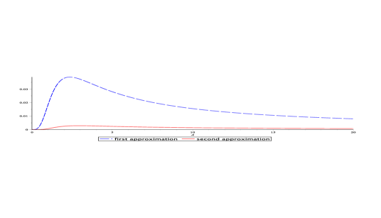
Figure 2.

Proof of Lemma 5.2.

The Hamiltonian function associated to (26) is $H(x,y)=y^{2}/2+x^{2}/2+x^{4}/4.$ The energy level is $H(x,y)=A^{2}/2+A^{4}/4:=h$. The expression of the period function is

$$T(A)=4\int_{0}^{A}\frac{dx}{\sqrt{2h-x^{2}-\frac{1}{2}x^{4}}}.$$

Making the change of variable $z=x/A$, we can write the above expression as

$$T(A)=\frac{4}{\sqrt{1+\frac{1}{2}A^{2}}}\int_{0}^{1}\frac{dz}{\sqrt{(1-z^{2})\left(1+\frac{A^{2}}{2+A^{2}}z^{2}\right)}},$$

which gives the expression (28) of $T$ that we wanted to prove. By using (27) and (28), straightforward computations yield to (29). The behavior at infinity of $T(A)$ is a direct consequence of Theorem 1.1 with $m=2$.

∎

Proof of Proposition 5.3.

Notice that result $(i)$ corresponds to the particular case $m=2$ in Proposition 1.2. In this case, expression (23) gives

$$T_{1}(A)=\frac{4\pi}{\sqrt{3A^{2}+4}}.$$

Straightforward computations show that its Taylor series at $A=0$ is (31). Moreover, writing $T_{1}(A)$ as

$$T_{1}(A)=\frac{4\pi}{A\sqrt{3+\frac{4}{A^{2}}}},$$

it is clear that $\frac{4\pi}{\sqrt{3}A}$ is its dominant term at infinity.

$(ii)$ System (26) is equivalent to the second order differential equation

$$\ddot{x}+x+x^{3}=0,$$ (36)

with initial conditions $x(0)=A$, $\dot{x}(0)=0$.

For applying second-order HBM we look for an solution of (36) of the form $x_{2}(t)=a_{1}\cos(\omega_{2}t)+a_{3}\cos(3\omega_{2}t)$ the above differential equation. The vanishing of the coefficients of $\cos(\omega_{2}t)$ and $\cos(3\omega_{2}t)$ in the Fourier series of $\mathcal{F}_{2}$ provides the non-linear system

$$-4\omega_{2}^{2}+3a_{1}^{2}+3a_{1}a_{3}+6a_{3}^{2}+4 =0,$$

$$-9a_{3}\omega_{2}^{2}+\frac{1}{4}a_{1}^{3}+\frac{3}{2}a_{1}^{2}a_{3}+a_{3}+\frac{3}{4}a_{3}^{3} =0.$$

From the initial conditions we have $a_{1}=A-a_{3}$. Hence the above system becomes

$$-4\omega_{2}^{2}+6a_{3}^{2}-3a_{3}A+3A^{2}+4 =0,$$

$$-9\omega_{2}^{2}a_{3}+2a_{3}^{3}-\frac{9}{4}a_{3}^{2}A+\frac{3}{4}a_{3}A^{2}+a_{3}+\frac{1}{4}A^{3} =0.$$

Doing the resultant of these equations with respect to $a_{3}$, we obtain the polynomial

$$1058\omega_{2}^{6}-3(219A^{2}+322)\omega_{2}^{4}-\frac{9}{4}(21A^{4}+80A^{2}+40)\omega_{2}^{2}-\frac{1323}{64}A^{6}-\frac{189}{4}A^{4}-27A^{2}-2.$$

Thus, $\omega_{2}$ is the unique real positive root of the above polynomial, that is,

$$\omega_{2}= \frac{\sqrt{2}}{92}\left(\frac{2166784+3272256\,A^{2}+1033992\,A^{4}+(1288+876A^{2})\,R^{1/3}+\,R^{2/3}}{R^{1/3}}\right)^{1/2}$$

where

$$R =3189506048+7956430848\,A^{2}+6507324864\,A^{4}+1763014086\,A^{6}$$

$$\,\,\quad+3174\,(320+357A^{2})\,A\,S,$$

$$S =(4521984+9925632\,A^{2}+6899904\,A^{4}+1559817\,A^{6})^{1/2}.$$

Therefore, the second approximation $T_{2}(A)$ to $T(A)$ of (26) is $T_{2}(A)=2\pi/\omega_{2}$, and it is not difficult to see that its Taylor series at $A=0$ is (33).

For studying the behavior of $T_{2}$ at infinity we rewrite $\omega_{2}$ as

$$\omega_{2}=\frac{\sqrt{2}\,A}{92\,\bar{R}^{1/6}}\left(\frac{2166784}{A^{4}}+\frac{3272256}{A^{2}}+1033992+\left(\frac{1288}{A^{4}}+\frac{876}{A^{2}}\right)\,\bar{R}^{1/3}+\,\bar{R}^{2/3}\right)^{1/2}$$

where

$$\bar{R} =\frac{3189506048}{A^{6}}+\frac{7956430848}{A^{4}}+\frac{6507324864}{A^{2}}+1763014086$$

$$\,\,\quad+\frac{1015680}{A^{5}}\bar{S}+1133118\bar{S},$$

$$\bar{S} =\left(\frac{4521984}{A^{6}}+\frac{9925632}{A^{4}}+\frac{6899904}{A^{2}}+1559817\right)^{1/2}.$$

From the previous expressions we have

$$\lim_{A\to\infty}\bar{S}=63\sqrt{393},\qquad\lim_{A\to\infty}\bar{R}=1763014086+71386434\sqrt{393}.$$

Thus,

$$\displaystyle\lim_{A\to\infty}\frac{2\pi A}{\omega_{2}}=\, \displaystyle\frac{92\sqrt{2}\pi\Delta}{\sqrt{1033992+876\Delta+\Delta^{2}}},$$

where $\Delta=(1763014086+71386434\sqrt{393})^{1/3}$.

Hence,

$$\lim_{A\to\infty}\frac{T_{2}(A)-\bar{\Delta}A^{-1}}{A^{-1}}=0,$$

where

$$\bar{\Delta}=\, \displaystyle\frac{92\sqrt{2}\pi\Delta}{\sqrt{1033992+876\Delta+\Delta^{2}}}.$$

Therefore, we have proved $(ii)$.

$(iii)$ When $N=3$ we look for a solution of (36) of the form $x_{2}(t)=a_{1}\cos(\omega_{3}t)+a_{3}\cos(3\omega_{3}t)+a_{5}\cos(5\omega_{3}t)$. Using the initial conditions we get that $a_{1}=A-a_{3}-a_{5}$. Afterwards, imposing that the first three significative harmonics vanish, we obtain the system of three equations:

$$P= A-{\omega_{3}}^{2}A+\frac{3}{4}{A}^{3}+\left({\omega_{3}}^{2}-\frac{3}{2}{A}^{2}-1\right)a_{{3}}+\left({\omega_{3}}^{2}-\frac{9}{4}{A}^{2}-1\right)a_{{5}}+\frac{9}{2}a_{{3}}a_{{5}}A$$

$$+\frac{9}{4}A{a_{{3}}}^{2}+{\frac{15}{4}}{a_{{5}}}^{2}A-\frac{9}{4}{a_{{5}}}^{3}-3{a_{{3}}}^{2}a_{{5}}-\frac{9}{2}a_{{3}}{a_{{5}}}^{2}-\frac{3}{2}{a_{{3}}}^{3}=0,$$

$$Q= \frac{1}{4}{A}^{3}+\left(1+\frac{3}{4}{A}^{2}-9{\omega_{3}}^{2}\right)a_{{3}}-\frac{3}{2}a_{{3}}a_{{5}}A-\frac{3}{4}{a_{{5}}}^{2}A-\frac{9}{4}A{a_{{3}}}^{2}$$

$$+\frac{3}{2}{a_{{3}}}^{2}a_{{5}}+\frac{9}{4}a_{{3}}{a_{{5}}}^{2}+2{a_{{3}}}^{3}+\frac{1}{2}{a_{{5}}}^{3}=0,$$

$$R= \frac{3}{4}{A}^{2}a_{{3}}+\left(-25{\omega_{3}}^{2}+\frac{3}{2}{A}^{2}+1\right)a_{{5}}-3{a_{{5}}}^{2}A-\frac{9}{2}a_{{3}}a_{{5}}A-\frac{3}{4}A{a_{{3}}}^{2}$$

$$+{\frac{15}{4}}{a_{{3}}}^{2}a_{{5}}+\frac{9}{4}{a_{{5}}}^{3}+{\frac{15}{4}}a_{{3}}{a_{{5}}}^{2}=0.$$

Since all the equations are polynomial, the searching of its solutions can be done by using successive resultants, see for instance [35]. We compute the following polynomials

$$PQ:=\frac{\operatorname{Res}(P,Q,a_{3})}{A-a_{5}},\quad QR:=\operatorname{Res}(Q,R,a_{3}),$$

and finally

$$PQR:=\frac{\operatorname{Res}(PQ,QR,a_{5})}{3A^{2}+4-36\omega_{3}^{2}}.$$

This last expression is a polynomial with rational coefficients that only depends on $A$ and $\omega_{3}$ and has total degree 70. Fortunately, it factorizes as $PQR(A,\omega_{3})=f(A,\omega_{3})g(A,\omega_{3}),$ with factors of respective degrees 22 and 48. Although both factors could give solutions of our system we continue our study only with the factor $f$. It is clear that if we consider the following numerator

$$h(A^{2},T^{2}):=\operatorname{Num}\Big{(}f\big{(}A,\frac{2\pi}{T}\big{)}\Big{)},$$

we have an algebraic curve $h(A^{2},T^{2})=0$ that gives a restriction that has to be satisfied in order to have a solution of our initial system. This function is precisely the one that appears in the statement of the proposition.

Once we have this explicit algebraic curve it is not difficult to obtain the other results of the statement. So, to obtain the local behavior near the origin we consider $T_{3}(A)=\sum_{k}^{m}t_{2k}A^{2k}$ and we impose that $h(A^{2},(T_{3}(A))^{2})\equiv 0$, obtaining easily the first values $t_{2k}.$ Similarly, for $A$ big enough, we impose that $T_{3}(A)\sim\delta/A$ obtaining the value of $\delta.$ ∎

6. Non-monotonous period function

In this section we study the family of systems (8) whose period function has a critical period (a maximum of the period function) and we show that the HBM also captures this behavior.

It is not difficult to establish the existence of values of $k\gtrsim-2$ for which the period function is not monotonous. It holds that, for all $k$,

$$\lim_{A\to 0}T(A)=2\pi\quad\mbox{and}\quad\lim_{A\to\infty}T(A)=0.$$ (37)

We remark that when $k\leq-2$ the center is no more global but there is also a neighborhood of infinity full of periodic orbits. When $k=-2$, the system has also the critical points $(\pm 1,0)$ and all the orbits of the potential system are closed, except the heteroclinic ones joining these two points. Hence, for $k=-2$ and from the continuity of the flow of (8) with respect to initial conditions, it follows that the periodic orbits close to these heteroclinic orbits have periods arbitrarily high; thus, the period of nearby periodic orbits, for $k>-2$ with $k+2$ small enough, is also arbitrarily high due to the continuity of the flow of (8) with respect to parameters. Therefore, from this property and (37) it follows that $T(A)$ is not monotonous.

The proof that $T(A)$ has only one maximum is much more difficult and indeed was the main objective of [25]. In that paper the authors proved this fact showing first that $T(h)$, where $h$ is the energy level of the Hamiltonian associated with (8), satisfies a Picard-Fuchs equation. As a consequence, the function $x(h)=T^{\prime}(h)/T(h)$ satisfies a Riccati equation. Finally, they study the flow of this equation for showing that $x(h)$ vanish at most at a single point.

Proof of Proposition 1.6.

For applying first-order HBM we write the family (8) as the second order differential equation

$$\ddot{x}+x+kx^{3}+x^{5}=0.$$

We look for a solution of the form $x_{1}(t)=a_{1}\cos(\omega_{1}t)$. The vanishing of the coefficient of $\cos(\omega_{1}t)$ in $\mathcal{F}_{1}$, and the initial conditions $x_{1}(0)=A>0$, $\dot{x}_{1}(0)=0$, provides the algebraic equation

$$16+12kA^{2}+10A^{4}-16\omega_{1}^{2}=0.$$

Solving for $\omega_{1}$ we obtain

$$\omega_{1}(A)=\frac{1}{4}\sqrt{16+12kA^{2}+10A^{4}}.$$

Then, the first approximation $T_{1}(A)$ to $T(A)$ is

$$T_{1}(A)=\frac{8\pi}{\sqrt{16+12kA^{2}+10A^{4}}},$$

which is well defined for all $A\in\mathbb{R}$ only for $k\in(-2\sqrt{10}/3,\infty)$. It is clear that if $k\geq 0$, then $T_{1}(A)$ is decreasing, which proves $(i)$. Moreover

$$T^{\prime}_{1}(A)={\frac{-16\pi\,A\left(3\,k+5\,{A}^{2}\right)}{\left(8+6\,k{A}^{2}+5\,{A}^{4}\right)\sqrt{16+12\,k{A}^{2}+10\,{A}^{4}}}}.$$

Hence, $T_{1}(A)$ has a non-zero critical point only when $k\in(-2\sqrt{10}/3,0)$, and it is $A=\sqrt{-3k}/\sqrt{5}$. Moreover, it is easy to see that such critical point is a maximum.

The proof of items (ii) and (iii) is straightforward. ∎

7. General potential system

In this section we consider the smooth potential system

$$\left\{\begin{array}[]{l}\dot{x}=-y,\\ \dot{y}=x+\displaystyle\sum_{i=2}^{\infty}k_{i}x^{i}.\end{array}\right.$$ (38)

Since its Hamiltonian function has a non degenerated minimum at the origin, it has a period annulus surrounding the origin. Thus, we have a period function $T(A)$ associated to this period annulus. The behavior near the origin of $T(A)$ is given in the following result.

Proposition 7.1.

The period function $T(A)$ of the system (38) at $A=0$ is

$$T(A)= 2\,\pi+\left(\frac{5}{6}\,{k_{2}}^{2}-\frac{3}{4}\,{k_{3}}\right)\pi{A}^{2}+\left(\frac{5}{9}\,{k_{2}}^{3}-\frac{1}{2}\,{k_{2}}\,{k_{3}}\right)\pi{A}^{3}$$

$$+\left(\frac{385}{288}k_{2}^{4}-\frac{275}{96}k_{2}^{2}k_{3}+\frac{7}{4}k_{2}k_{4}+\frac{57}{128}k_{3}^{2}-\frac{5}{8}k_{5}\right)\pi A^{4}+O\left({A}^{5}\right).$$

The proof of this proposition follows by using standard methods in the local study of the period function [9, 20].

By applying the HBM to the next family of potential systems

$$\left\{\begin{array}[]{l}\dot{x}=-y,\\ \dot{y}=x+\displaystyle\sum_{i=2}^{M}k_{i}x^{i},\end{array}\right.$$ (39)

for $M=3,4,5,6,7,$ we obtain the corresponding $T_{1,M}(A)$ which satisfy

$$T_{1,M}(A)=2\,\pi+\left({k_{2}}^{2}-\frac{3}{4}\,{k_{3}}\right)\pi{A}^{2}+O_{M}\left({A}^{3}\right).$$

As can be seen, the quadratic terms do not depend on $M$. These first terms only coincide with the corresponding ones of $T(A)$ when $k_{2}=0$. Notice that this is the situation in Propositions 1.6 and 5.3.

To get a more accurate approach of $T(A)$ we have applied the second order HBM to (39) with $M=3$ obtaining

$$T_{2}(A)=2\,\pi+\left(\frac{5}{6}\,{k_{2}}^{2}-\frac{3}{4}\,{k_{3}}\right)\pi{A}^{2}+O\left({A}^{3}\right),$$

result that coincides with the actual value of $T(A)$.

Conclusions

Studying several examples of potential systems we have seen that the approximations $T_{N}(A)$ calculated using the $N$-th order HBM keep some of the properties (analytic and qualitative) of the actual period function $T(A)$. Moreover, this matching seems to improve when $N$ increases.

We believe that obtaining general results to strengthen the above relationship is a challenging question.

Acknowledgements

The two authors are supported by the MICIIN/FEDER grant number MTM2008-03437 and the Generalitat de Catalunya grant number 2009-SGR 410. The first author is also supported by the grant AP2009-1189.

References

• [1]
• [2] M. Abramowitz, I. A. Stegun, “Handbook of Mathematical Functions with Formulas, Graphs, and Mathematical Tables” New York: Dover, eds. (1965).
• [3] A. Beléndez, E. Gimeno, M. L. Álvarez, M. S. Yebra, D. I. Méndez, Analytical approximate solutions for conservative nonlinear oscillators by modified rational harmonic balance method, Int. J. Comput. Math. 87 (2010), 1497–1511.
• [4] A. Beléndez, E. Gimeno, T. Beléndez, A. Hernández, Rational harmonic balance based method for conservative nonlinear oscillators: application to the Duffing equation, Mech. Res. Comm. 36 (2009), 728–734.
• [5] O. A. Chalykh, A. P. Veselov, A remark on rational isochronous potentials, J. Nonlinear Math. Phys. 12 (2005), suppl. 1, 179–183.
• [6] L. A. Cherkas. Number of limit cycles of an autonomous second-order system, Differential Equations 5 (1976) 666–668.
• [7] C. Chicone, The monotonicity of the period function for planar Hamiltonian vector fields, J. Differential Equations 69 (1987), 310 -321.
• [8] C. Chicone, Geometric methods of two-point nonlinear boundary value problem, J. Differential Equations 72 (1988), 360–407.
• [9] C. Chicone, M. Jacobs, Bifurcation of critical periods for plane vector fields, Trans. Amer. Math. Soc. 312 (1989), no. 2, 433–486.
• [10] S. N. Chow and J. K. Hale, Methods of bifurcation theory. Grundlehren der Mathematischen Wissenschaften [Fundamental Principles of Mathematical Science], 251. Springer-Verlag, New York-Berlin, 1982.
• [11] C. J. Christopher, J. Devlin, Isochronous centers in planar polynomial systems, SIAM J. Math. Anal. 28 (1997), 162 -177.
• [12] A. Cima, A. Gasull, F. Mañosas, Period function for a class of Hamiltonian systems, J. Differential Equations 168 (2000), 180–199.
• [13] A. Cima, F. Mañosas, J. Villadelprat, Isochronicity for several classes of Hamliltonian systems, J. Differential Equations 157 (1999), no. 2, 373 -413.
• [14] A. Constantin and G. Villari, Particle trajectories in linear water waves, J. Math. Fluid Mech. 10 (2008), 1–18.
• [15] S. Foschi, G. Mingari Scarpello, D. Ritelli, Higher order approximation of the period-energy function for single degree of freedom Hamiltonian systems, Meccanica 39 (2004), 357 -368.
• [16] E. Freire, A. Gasull, A. Guillamon, First derivative of the period function with applications, J. Differential Equations 204 (2004) 139–162.
• [17] J. D. García-Saldaña, A. Gasull, A theoretical basis for the harmonic balance method, J. Differential Equations 254 (2013), 67 -80.
• [18] A. Garijo, A. Gasull, X. Jarque, On the period function for a family of complex differential equations, J. Differential Equations 224 (2006), 314–331.
• [19] A. Gasull, A. Guillamon, J. Villadelprat, The period function for second-order quadratic ODEs is monotone, Qual. Theory Dyn. Syst. 4 (2004), no. 2, 329–352.
• [20] A. Gasull, A. Guillamon, V. Mañosa, An explicit expression of the first Liapunov and period constants with applications, J. Math. Anal. Appl. 211 (1997), no. 1, 190–212.
• [21] A. Gasull, C. Liu, J. Yang, On the number of critical periods for planar polynomial systems of arbitrary degree, J. Differential Equations 249 (2010) 684 692
• [22] M. Gavrilov, Isochronicity of plane polynomial Hamiltonian systems, Nonlinearity 10 (1997), 433 -448.
• [23] H. Hu, J. H. Tang, Solution of a Duffing-harmonic oscillator by the method of harmonic balance, J. Sound Vibration 294 (2006), 637 -639.
• [24] C. W. Lim, B. S. Wu, A new analytical approach to the Duffing-harmonic oscillator, Phys. Lett. A 311 (2003), 365–373.
• [25] F. Mañosas, J. Villadelprat, A note on the critical periods of potential systems, Internat. J. Bifur. Chaos Appl. Sci. Engrg. 16 (2006), 765–774.
• [26] P. Mardesic, C. Rousseau, B. Toni, Linearization of isochronous centers, J. Differential Equations 121 (1995), 67- 108.
• [27] M. Momeni, N. Jamshidi, A. Barari, D. D. Ganji, Application of He’s energy balance method to Duffing-harmonic oscillators, Int. J. Comput. Math. 88 (2011), 135–144.
• [28] R. E. Mickens, A generalization of the method of harmonic balance, J. Sound Vibration 111 (1986), 515–518.
• [29] R. E. Mickens, “Oscillations in planar dynamic systems”, Series on Advances in Mathematics for Applied Sciences, 37. World Scientific Publishing Co., Inc., River Edge, NJ, 1996.
• [30] R. E. Mickens, Mathematical and numerical study of the Duffing-harmonic oscillator, J. Sound Vibration 244 (2001), 563 -567.
• [31] R. E. Mickens, Harmonic balance and iteration calculations of periodic solutions to $\ddot{y}+y^{-1}=0$, J. Sound Vibration 306 (2007), 968–972.
• [32] R. E. Mickens, “Truly nonlinear oscillations. Harmonic balance, parameter expansions, iteration, and averaging methods”, World Scientific Publishing Co. Pte. Ltd., Hackensack, NJ, 2010.
• [33] F. Rothe, The periods of the Volterra-Lotka system, J. Reine Angew. Math. 355 (1985), 129–138.
• [34] M. Sabatini, On the period function of Liénard systems, J. Differential Equations 152 (1999), 467- 487.
• [35] B. Sturmfels, “Solving systems of polynomial equations”. CBMS Regional Conference Series in Mathematics 97. Published for the Conference Board of the Mathematical Sciences, Washington, DC; by the American Mathematical Society, Providence, RI, 2002.
• [36] J. Waldvogel, The period in the Lotka-Volterra system is monotonic, J. Math. Anal. Appl. 114 (1986), 178–184.
• [37] J. Zhang, Limit cycle for the Brusselator by He’s variational method, Math. Probl. Eng. 2007, Art. ID 85145, 8 pp.
• [38] Y. Zhao, The monotonicity of period function for codimension four quadratic system $Q_{4}^{1}$, J. Differential Equations 185 (2002), 370- 387.