Absorption and eigenmode calculation for one-dimensional periodic metallic structures using the hydrodynamic approximation

Abstract

We develop a modal method that solves Maxwell’s equations in the presence of the linearized hydrodynamic correction. Using this approach, it is now possible to calculate the full diffraction for structures with period of the order of the plasma wavelength, including not only the transverse but also the longitudinal modes appearing above the plasma frequency. As an example for using this method we solve the diffraction of a plane wave near the plasma frequency from a bi-metallic layer, modeled as a continuous variation of the plasma frequency. We observe absorption oscillations around the plasma frequency. The lower frequency absorption peaks and dips correspond to lowest longitudinal modes concentrated in the lower plasma frequency region. As the frequency is increased, higher order longitudinal modes are excited and extent to the region of higher plasma frequency. Moreover, examination of the propagation constants of these modes reveals that the absorption peaks and dips are directly related to the direction of phase propagation of the longitudinal modes. Furthermore, we formulate a variant of the Plane Wave Expansion method, and use it to calculate the dispersion diagram of such longitudinal modes in a periodically modulated plasma frequency layer.

I introduction

Along with advances in nano-plasmonics, plasmonic devices reach length scales for which non-local effects of the metal electric permittivity function may no longer be neglected. For noble metals with critical dimensions in the sub-10 nm regime, the longitudinal plasmonic response exhibits spatial dispersion. This deviation from the ordinary local approximation, requires modification of known analytical and numerical tools. The hydrodynamic non-local model forstmann-book ; boardman-book ; pitarke ; feibelman can be regarded as a simple approach (compared to more complex, quantum models). However, it successfully reproduces experimental results obtained for thin layered metals Anderegg and offers a qualitative explanation for the blue shifting of the localized surface-plasmon resonance observed in silver nanoparticles ciraci ; raza2 . These results can not be explained with local models. In this paper, we study the response of a metallic layer with periodic variation of the free-carrier density, under the hydrodynamic approximation. While the hydrodynamic model fails to account for quantum-size effects, such as quantum tunneling stella-hydro-quantum ; teperik-quantum-corrected ; esteban-quantum-corrected , it is a well established model for the dimensions studied here. Until now, various numerical algorithms that solve Maxwell’s equations with the hydrodynamic correction have been reported toscano ; ruppin-1 ; hiremath ; yannopapas ; mochan-tmm ; deabajo ; fernandez-dominguez ; raza ; toscano-2 . In this paper, we provide a rigorous numerical approach, that allows the calculation of 1D periodic structures. Our method relies on the Fourier Modal Method (FMM) also known as the Rigorous Coupled Wave Analysis (RCWA) method moharam ; lalanne ; lifengli2 . This method can be regarded as semi-analytic in the sense that not only the field distribution is calculated, but also the propagation constants and the eigenmodes of the periodic structure are obtained, allowing to derive additional physical insight (see e.g. lalanne-2 ). Adding the hydrodynamic terms to the ordinary FMM formulation, allows us to utilize some of the strengths that are offered by FMM. The paper is structured as follows. In Section II the FMM with the additional hydrodynamic terms is presented. In addition, we formulate the band diagram dispersion calculation of the longitudinal modes. In Section III, results based on this framework are shown. Section IV concludes the paper.

II FMM with the hydrodynamic correction

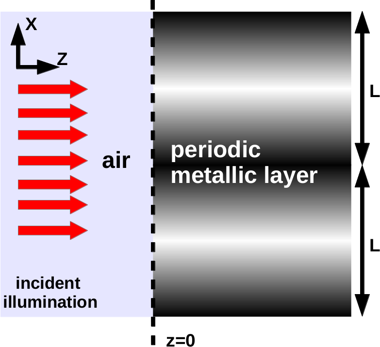
Figure 1: Schematic showing two unit cells of the diffraction problem geometry, with light incident from left to right. The air/metal interface is located at z=0, and the direction of periodicity is along the vertical (i.e. x) axis. The region with reduced free-carrier density is in the center of the unit cell (bright), whereas the boundaries of the unit cell are the region with higher free-carrier density (dark).

First, we briefly review the essential basics of the FMM. Further details can be found in several references, e.g. moharam ; lalanne . In its most common formulation, the FMM uses a Floquet-Bloch expansion within a unit cell $0\leq x<L$ (see schematic in Fig. 1), to represent Maxwell’s equations in each z-invariant periodic layer. Afterwards, the eigenmodes and eigenvalues of the fields are calculated by solving an eigenvalue equation. We now elaborate on these principles. The Floquet-Bloch condition implies that the wavevectors in the $x$ direction are given by $k_{x,m}=k_{x,0}+mK$, where $K=2\pi/L$ is the grating vector and $k_{x,0}$ is the “zero-order” term. With the FMM, Maxwell’s equations are solved for each locally z-invariant layer, from an eigenvalue equation of the form $\frac{\partial}{\partial z}\mathbf{F}=\mathbf{A}\,\mathbf{F}$. Here, $\mathbf{F}$ is a column vector of the Fourier components of the fields and $\mathbf{A}$ is an operator matrix defined by Maxwell’s equations. The propagation constants $k_{z,n}$, are obtained by solving this eigenvalue equation. In order to solve the eigenvalue equation numerically, one must truncate the number of Fourier components to some finite number of $N$ elements, with $-\left\lfloor N/2\right\rfloor\leq m\leq\left\lfloor N/2\right\rfloor$. Generally, the solution converges to the exact solution by increasing $N$. In order to solve a diffraction problem, the fields in adjacent layers are matched by employing the proper boundary conditions. By this matching procedure, a mode amplitude constant $C_{n}$ is solved for the $n^{th}$ eigenmode moharam . In the following subsection we present the derivation of the matrix operator $\mathbf{A}$ in the presence of the hydrodynamic correction.

II.1 Maxwell’s equations with the hydrodynamic correction

In each z-invariant layer, and for a single frequency component $\omega$, Maxwell’s equations with the linearized hydrodynamic correction are given by boardman-ruppin ; hiremath :

$$\nabla\times E-j\omega\mu_{0}H = 0$$ (1a)

$$\nabla\times H+j\omega\varepsilon_{0}E+eN_{0}(x)v = 0$$ (1b)

$$\varepsilon_{0}\nabla\cdot E+en_{1} = 0$$ (1c)

$$\nabla\cdot\left[N_{0}(x)v\right]-j\omega n_{1} = 0$$ (1d)

$$-jm\omega(N_{0}(x)v)+m\gamma(N_{0}(x)v)+N_{0}(x)eE+m\beta^{2}\nabla n_{1} = 0$$ (1e)

where $N_{0}(x)$ is a periodic function of the density of free electrons in equilibrium, $n_{1}$ is the first-order non-equilibrium correction to the equilibrium electron density and likewise $v$ is the first-order non-equilibrium electron velocity while there are no equilibrium currents. Furthermore, the strength of the non-local response is governed by $\beta^{2}=\frac{3}{5}v_{F}^{2}$. The electron mass is denoted by $m$. The case that $N_{0}$ varies with $x$ while $\beta$ is constant, can be regarded as a toy model for the scenario in which two metals with different plasma frequencies fill the unit cell, with continuous variation of the free carrier density. We solve the set of Eq. (1) for TM polarization [i.e. $H(x,y,z)=\hat{y}H_{y}(x,z)$ and $E(x,y,z)=\hat{x}E_{x}(x,z)+\hat{z}E_{z}(x,z)$], as only this polarization supports longitudinal modes. As explained above, in order to solve Eq. (1) with standard FMM formulation, we need to isolate all $\frac{\partial}{\partial z}$ dependencies to obtain an eigenvalue equation. For convenience, we introduce $\hat{\omega}^{2}=\omega(\omega+i\gamma),\>\tilde{\beta}^{2}=\beta^{2}/c^{2},\tilde{\>\omega}_{p}^{2}=\omega_{p}^{2}/c^{2}=\frac{N_{0}e^{2}}{m\varepsilon_{0}}/c^{2},\>\hat{k}_{0}=\hat{\omega}/c,\hskip 10.00002pt\tilde{\mu}_{0}=c\mu_{0}\text{, and }\tilde{\varepsilon}_{0}=c\varepsilon_{0}=\tilde{\mu}_{0}^{-1}.$ Furthermore, we define the hydrodynamic current as $J=eN_{0}v$ and $J(x,y,z)=\hat{x}J_{x}(x,z)+\hat{z}J_{z}(x,z)$. Since we have spatial harmonic variations, we straightforwardly make the following substitutions for the derivatives: $\partial/\partial_{z}=jk_{0}k_{z}$ and $\partial/\partial_{x}=jk_{0}k_{x}$. Making these substitutions and performing algebraic manipulations described in some detail in Appendix A, we arrive at the eigenvalue equation in matrix form:

$$\left[\begin{array}[]{c}\mathbf{E_{x}}\\ \mathbf{\nabla\cdot J}\end{array}\right]\left[\mathbf{K_{z}^{2}}\right]=\left[\begin{array}[]{cc}\tilde{\mu}_{0}\mathbf{I}&\mathbf{K_{x}}\\ \hat{k}_{0}^{2}\tilde{\beta}^{-2}\mathbf{K_{x}}&\tilde{\varepsilon}_{0}\tilde{\beta}^{-2}\left(\hat{k}_{0}^{2}\mathbf{I}-\mathbf{\Omega_{p}^{2}}\right)\end{array}\right]\left[\begin{array}[]{cc}\tilde{\varepsilon}_{0}\hat{k}_{0}^{-2}\left(\hat{k}_{0}^{2}\mathbf{I}-\mathbf{\Omega_{p}^{2}}\right)&-\hat{k}_{0}^{-2}\tilde{\beta}^{2}\mathbf{K_{x}}\\ -\mathbf{K_{x}}&\tilde{\mu}_{0}k_{0}^{-2}\mathbf{I}\end{array}\right]\left[\begin{array}[]{c}\mathbf{E_{x}}\\ \mathbf{\nabla\cdot J}\end{array}\right]$$ (2)

Here, $\mathbf{E_{x}}$ and $\mathbf{\nabla\cdot J}$ are the eigenvector matrices of $E_{x}$ and $\nabla\cdot J$ respectively. $\mathbf{K_{x}}$ and $\mathbf{K_{z}}$ are diagonal matrices with elements $k_{x,m}$ and $k_{z,n}$ respectively, and the identity matrix is $\mathbf{I}$. $\mathbf{\Omega_{p}^{2}}$ is the Toeplitz matrix with elements corresponding to the Fourier components of $\tilde{\omega}_{p}^{2}(x)$. The matrices $\mathbf{I}$ , $\mathbf{\Omega_{p}^{2}}$ , $\mathbf{K_{x}}$, $\mathbf{E_{x}}$ and $\mathbf{\nabla\cdot J}$ are of size $N\times N$ , while $\mathbf{K_{z}}$ is a $2N\times 2N$ matrix and the overall number of eigenmodes obtained from Eq. (2) is $2N$. However, in local media, the number of eigenmodes is equal to the truncation number i.e. $N$ moharam . Therefore, a total of $3N$ mode amplitude constants need to be found when matching the fields at the interface of a local layer with a layer with non-local response. The ordinary boundary conditions demanding continuity of the tangential field components $E_{x}$ and $H_{y}$ provide only $2N$ equations. To match the “missing” $N$ amplitude constants, an additional boundary condition (ABC) is required. This is very similar to the known case of matching the field amplitudes between two homogeneous local and non-local layers melnyk . For simplicity, we consider an air/metal interface. For this case, the boundary conditions are the continuity of $E_{x}$, $J_{z}$ and $E_{z}$ across the interface forstmann-book ; yan-hyperbolic ; moreau . We note however, that the ABC does not change in any way the eigenvalue equation of the periodic metallic layer, which is a direct solution of Maxwell’s equations with the hydrodynamic correction. In Section III.1, we solve a full diffraction problem for the case of light incident from air on a semi-infinite periodic non-local layer. At the interface of both media, the mode amplitude constants are found by employing these boundary conditions. In Appendix B, we present a procedure based on the S-matrix algorithm lifengli2 , for the calculation of the mode amplitudes. For completeness, this procedure is formulated for the more general case of a non-local periodic layer embedded in a local environment.

II.2 Band diagram calculation

In order to calculate the dispersion diagram of the longitudinal modes, we follow an approach based on that in dispersive-band-diagram . This approach is a variant of the Plane Wave expansion Method (PWM) photonics-crystal-book . In contrast to the conventional PWM, where the Bloch wavevector ($k_{x,0}$) is assumed and the frequency ($\omega$) is solved from an eigenvalue problem, in the revised PWM, the frequency is assumed beforehand, and the phase difference of the fields across the unit cell (known as the Bloch wavevector) is calculated. We note that for nondispersive loss-less materials there is a freedom to choose one or the other. However, for the dispersive metal it is important that one solves for the complex Bloch wave vector while treating the frequency as real (alternatively, one can also solve for complex $\omega$, see Ref. fan ) . This is relevant for the experimental situation where the structure is probed by a CW laser with a well-defined frequency. We now show how the PWM variant can be applied to calculate the dispersion diagram of a metallic structure with the hydrodynamic correction. For simplicity, we assume a 1D case with $k_{z}=0$ , and that $\omega_{p}$ is periodic with $x$. For such a case, Eq. (1) (see also Eq. (A)) reduces to three first order differential equations:

$$k_{x}E_{z}+\tilde{\mu}_{0}H_{y} = 0$$ (3a)

$$\tilde{\varepsilon}_{0}\varepsilon_{T}E_{z}+k_{x}H_{y} = 0$$ (3b)

$$E_{x}-\hat{k}_{0}^{-2}\tilde{\omega}_{p}^{2}(x)E_{x}-\hat{k}_{0}^{-2}k_{0}^{2}\tilde{\beta}^{2}k_{x}^{2}E_{x}=0$$ (3c)

Here $\varepsilon_{T}\equiv 1-\frac{\tilde{\omega}_{p}^{2}(x)}{\hat{k}_{0}^{2}}.$ Eq. (3) can be subdivided into two independent sets: Eq. (3a) and (3b) describe the transverse modes (no field components in the direction of the only non-zero k-vector component, i.e. $k_{x})$ while Eq. (3c) defines the dispersion law of the longitudinal modes. Moreover, by defining $\varepsilon_{L}\equiv 1-\frac{\tilde{\omega}_{p}^{2}(x)}{\hat{k}_{0}^{2}-k_{0}^{2}\tilde{\beta}^{2}k_{x}^{2}}$, Eq. (3c) can be re-written as $\varepsilon_{L}E_{x}=0$, from which the familiar condition for longitudinal modes $\varepsilon_{L}=0$ is apparent. To solve Eq. (3c), we define $k_{x}\equiv k_{x,0}+k_{x,m}$. Here $k_{0}k_{x,0}L$ is the phase difference of the field $F$ between the two boundaries of the unit cell according to: $F(x=L)=F(x=0)\exp(jk_{0}k_{x,0}L)$, and $k_{x,m}=mK$. With these definitions, and the auxiliary field quantity $\dot{E}_{x}\equiv\left[k_{x,0}+k_{x,m}\right]E_{x}$, we split Eq. (3c) into two first order equations

:

$$\tilde{\beta}^{-2}k_{0}^{-2}\left(\hat{k}_{0}^{2}-\tilde{\omega}_{p}^{2}(x)\right)E_{x}-\left[k_{x,0}+k_{x,m}\right]\dot{E}_{x}=0$$ (4a)

$$\dot{E}_{x}=\left[k_{x,0}+k_{x,m}\right]E_{x}$$ (4b)

Eq. (4) can be recast to the matrix form:

$$\left[\begin{array}[]{c}\mathbf{\dot{E}_{x}}\\ \mathbf{E_{x}}\end{array}\right]\left[\mathbf{K_{x,0}}\right]=\left[\begin{array}[]{cc}-\mathbf{K_{x}}&\tilde{\beta}^{-2}k_{0}^{-2}\left(\hat{k}_{0}^{2}\mathbf{I}-\mathbf{\Omega_{p}^{2}}\right)\\ \mathbf{I}&-\mathbf{K_{x}}\end{array}\right]\left[\begin{array}[]{c}\mathbf{\dot{E}_{x}}\\ \mathbf{E_{x}}\end{array}\right]$$ (5)

Here $\mathbf{K_{x,0}}$ is a $2N\times 2N$ diagonal matrix with elements corresponding to the phase difference between the boundaries of the unit cell of each eigenmode, and $\mathbf{K_{x}}$ is an $N\times N$ diagonal matrix with elements $k_{x,m}=mK$. Eq. (5) can be identified as an eigenvalue equation from which the matrix of phase constants $\mathbf{K}_{\mathbf{x,0}}$ can be obtained.

III Simulation results

III.1 Absorption spectrum of a semi-infinite metallic layer with sinusoidal modulation of $\omega_{p}$

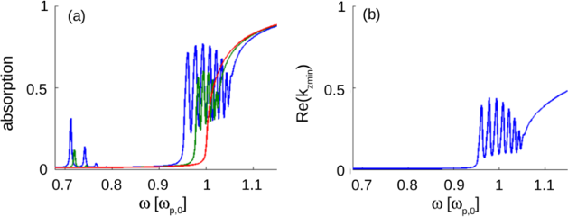
Figure 2: (a) Absorption spectrum of a semi-infinite metallic layer with $\lambda_{p}=\frac{2\pi c}{\omega_{p,0}}=5L$. Blue line, $\omega_{p,1}^{2}=0.1\omega_{p,0}^{2}.$ Green line $\omega_{p,1}^{2}=0.05\omega_{p,0}^{2}$. Red line: $\omega_{p,1}^{2}=0$ (b) Real part of the propagation constant with absolute value closest to zero, calculated for the case that $\omega_{p,1}^{2}=0.1\omega_{p,0}^{2}.$

As first application of the modified FMM, we first consider the following toy geometry: A TM plane wave is normally incident upon a semi-infinite metallic layer, with modulation of the plasma frequency given by: $\omega_{p}^{2}=\omega_{p,0}^{2}+\omega_{p,1}^{2}\cos(\frac{2\pi x}{L})$. The material parameters are $\gamma=\omega_{p,0}/300$, $v_{F}=0.01c$ and $\lambda_{p}\equiv\frac{2\pi c}{\omega_{p,0}}=5L$. The calculation has been repeated for the following three modulation amplitudes: $\omega_{p,1}^{2}=0.1\omega_{p,0}^{2},$ $0.05\omega_{p,0}^{2}$ and 0. The results are shown in Fig. 2(a). Two sets of absorption peaks are observed: 1) Absorption peaks near the frequencies $\sim\left(1/\sqrt{2}\right)\omega_{p,0}$ . These are surface waves (surface plasmon polariton (SPP) like) that are confined near the interface. 2) Absorption oscillations appearing near $\omega_{p,0}$ , which are the consequence of longitudinal waves. It is seen that the oscillation strength increases as the plasma frequency modulation amplitude increases. In Fig. 3(a,b) we plot $\nabla\cdot J,$ for the two lowest frequency absorption peaks ($\frac{\omega}{\omega_{p,0}}=\text{0.9605 and 0.9772})$, and in Fig. 3(c,d) we plot the same quantities for the first two absorption dips ($\frac{\omega}{\omega_{p,0}}=\text{ 0.9674 and 0.9841})$ . Since $\nabla\cdot J$ is proportional to the induced charge density (see Eq. (1d)), it can be seen that for the lower frequency modes, the induced charge density concentrates in the middle of the unit cell where the plasma frequency is minimal. This is consistent with previous studies where a layer of metal with lower plasma frequency was deposited on top of a higher plasma frequency metal. For such a case, standing waves in the lower plasma frequency region, similar to those in a 1D potential well were observed (see Ref. forstmann-book section 3.4). In addition, calculation of $H_{y}$ which is a transverse field quantity (no magnetic field exists in a longitudinal mode), shows that the magnetic field is negligible compared to $\nabla\cdot J$, manifesting that the modes are almost completely longitudinal in nature. To reveal the reason for the existence of the absorption peaks and dips, we plot in Fig. 2(b) the real part of the propagation constant with absolute value closest to zero as a function of frequency, for the case that $\omega_{p,1}^{2}=0.1\omega_{p,0}^{2}.$ More mathematically stated, we define $k_{z,\text{min}}$ $\equiv\text{min}(|k_{z,n}|^{2})$ and plot Re$(k_{z,\text{min}})$. There is a clear correspondence between the blue line in Fig. 2(a) and Fig. 2(b). The dips and peaks of the absorption spectrum are located at the minimas and the maximas of Re$(k_{z,\text{min}})$ respectively. The reason for this is that when Re$(k_{z})$ is relatively large, the longitudinal mode propagates with significant phase accumulation along the $z$ axis and eventually dissipates. On the other hand, when Re$(k_{z})\cong 0$, the longitudinal mode barely propagates into the metal, but rather has a standing wave pattern along the $x$ axis (Supplemental Material supplemental-material ). This analysis shows the strength of the FMM approach. Being a semi-analytical method, it provides physical insight due to the calculation of modes and propagation constants.

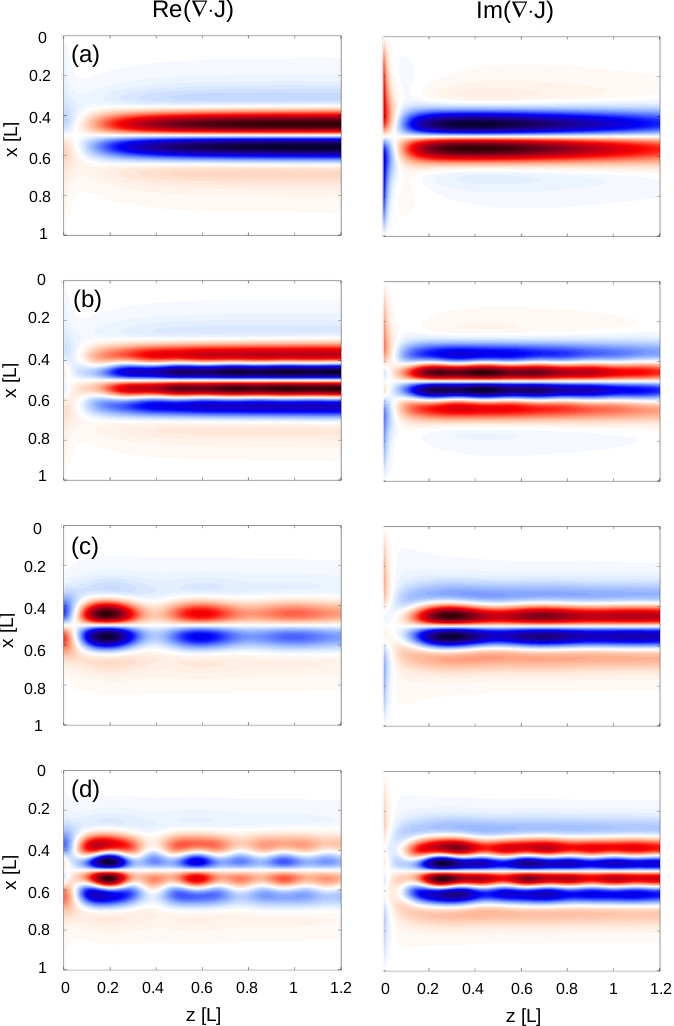
Figure 3: (a,b) Real and imaginary parts of $\nabla\cdot J$, calculated at the absorption peaks, located at (a) $\frac{\omega}{\omega_{p,0}}=\text{0.9605 and (b) $\frac{\omega}{\omega_{p,0}}$=0.9772 }$. (c,d) Real and imaginary parts of $\nabla\cdot J$, calculated at the absorption dips, located at (c) $\frac{\omega}{\omega_{p,0}}=\text{0.9674 and (d) $\frac{\omega}{\omega_{p,0}}$=0.9841 }$ The air/metal interface is at z=0.

III.2 Absorption spectrum of an Au/Ag bi-metallic semi-infinite layer

We now turn to analyze the case of an Au/Ag semi-infinite layer. We assume $\omega_{p,\text{Au}}=8.55$[eV], $\omega_{p,\text{Ag}}=9.6$[eV], $\gamma_{\text{Au}}=\gamma_{\text{Ag}}=0.02$[eV] and $v_{F,\text{Au}}=v_{F,\text{Ag}}=0.0047c$. These parameters are from blaber , with the simplifying assumption that the damping in Au and Ag is the same. In the unit cell $0\leq x<L$, the plasma frequency is described by: $\omega_{p}^{2}(x)=\text{arctan}\left[(x-0.5L)(f/L)\right]\left(\omega_{p,\text{Au}}^{2}-\omega_{p,\text{Ag}}^{2}\right)/\pi+\left(\omega_{p,\text{Au}}^{2}+\omega_{p,\text{Ag}}^{2}\right)/2$. This function results in continuous step-like profile. The advantage of using such function is that it eliminates the need to take care of the correct factorization rules of a piecewise discontinuous function lifengli ; lalanne , and also provides a more realistic description of the transition between the two metals. The parameter $f$ determines the steepness of the transition between both media. In Fig. 4(a) we plot the absorption spectrum, for $f=100$ and $L=$35[nm] . The step-like distribution of $\omega_{p}$ in the unit cell is shown in Fig. 4(c). Similarly to the case studied in Section III.1, the absorption spectrum exhibts peaks near $\left(1/\sqrt{2}\right)\omega_{p,\text{Au}}$ and $\left(1/\sqrt{2}\right)\omega_{p,\text{Ag}}.$ Additionaly, there are absorption peaks due to longitudinal modes for $\omega_{p,\text{Au}}<\omega<\omega_{p,\text{Ag}}$. The reason no absorption peaks are observed for $\omega>\omega_{p,\text{Ag}}$, is that the unit cell is larger than the typical dimension ($\sim$10 [nm]) for which non-local effects are significant for these metals. However, when $\omega_{p,\text{Au}}<\omega<\omega_{p,\text{Ag}}$, longitudinal modes exist only in the Au layer, which for the assumed unit cell size, is small enough to clearly observe longitudinal resonances. Indeed, for a smaller unit cell with $L=10$[nm], resonances of longitudinal modes for $\omega>\omega_{p,\text{Ag}}$ are observed (see Fig. 4(b)). In Fig. 4(d), we show $\nabla\cdot J$ calculated for $\omega=8.592$ [eV] and $L=35$[nm]. It can be observed that the longitudinal modes are confined in the Au layer only.

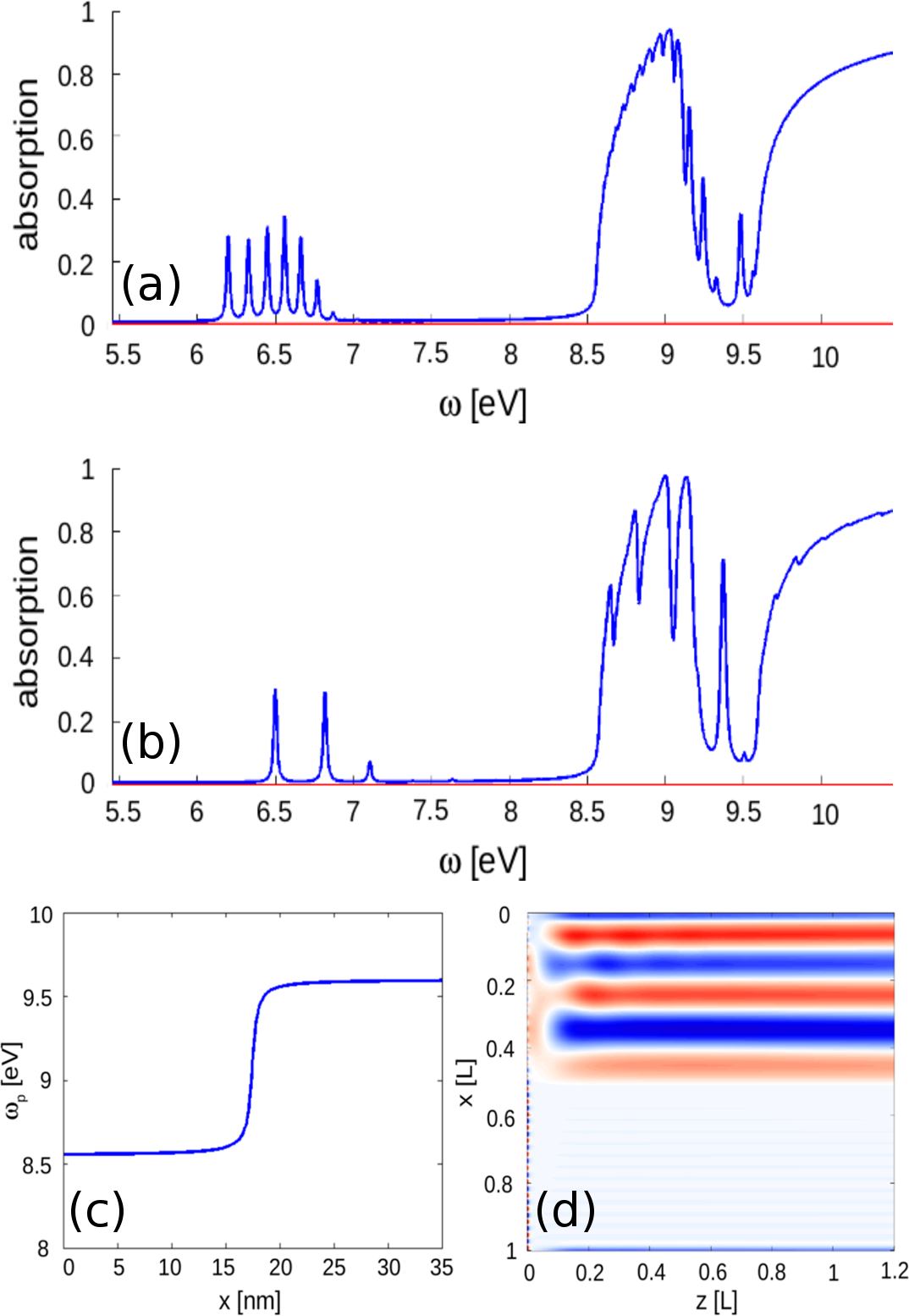
Figure 4: (a) Absorption spectrum of an Ag/Au grating with $L=$35[nm] as function of $\omega$. (b) Absorption spectrum of an Ag/Au grating with $L=$10[nm] as function of $\omega$. (c) The distribution of $\omega_{p}$ in the unit cell assumed for the calculation. (d) The real part of $\nabla\cdot J$, calculated for $\omega=8.592$[eV] and $L=$35[nm].

III.3 Band diagram calculation

We now turn into calculating the 1D dispersion diagram of longitudinal modes, based on the formulation described in Section II.2. We assume the following parameters: $\gamma=0$ (no losses), $v_{F}=0.01c$ and $\lambda_{p}=\frac{2\pi c}{\omega_{p,0}}=10L$.

Figure 5: Dispersion of the longitudinal modes. (a) periodic case with $\omega_{p,1}^{2}=0.02\omega_{p,0}^{2}$. (b) uniform case $(\omega_{p,1}^{2}=0)$

In Fig. 5(a) we assumed $\omega_{p,1}^{2}=0.02\omega_{p,0}^{2}$. For this case both the band gaps at the edges of the 1st Brillouin Zone (BZ) and at $k_{x,0}=0$ are apparent. Moreover, the dispersion of the lower order modes is flat, which is an indication for a very low group velocity, regardless of the specific momentum value. This is in contrast to the more conventional case of a periodic structure which generates slow light only at the edges of the BZ. Losses (neglected here for simplicity) however, cause broadening and enhance the group velocity at the band edges slow-light-band . In 5(b) we assumed a uniform metallic medium having no modulation, i.e. $\omega_{p,1}^{2}=0$. Obviously, for this case, no bandgaps are observed, as expected.

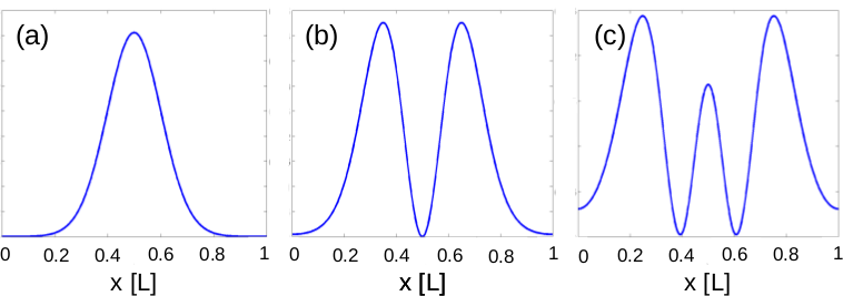
Figure 6: The profile of $|J_{x}|^{2}$ for the 1st - 3rd bands of the dispersion diagram plotted in Fig. 5(a). (a) $\omega=0.9936\omega_{p,0}$ (b) $\omega=1.0005\omega_{p,0}$ (c) $\omega=1.0064\omega_{p,0}$ . All modes are calculated for $k_{x,0}=0.$

In Fig. 6 we plot the mode profile of $|J_{x}(x)|^{2}$ (which is proportional to the kinetic energy of the charges) for the three first bands of the dispersion diagram plotted in Fig. 5(a). As discussed before, it is seen that the lowest energy mode is concentrated in the region of smaller plasma frequency.

IV Conclusion

In summary, we have developed a semi-analytical modal approach to solve Maxwell’s equations in the presence of the linearized hydrodynamic correction. With this approach, the diffraction from a periodic metallic layer was calculated. The modal method was shown to provide physical insight to the calculated absorption spectrum, by detailed inspection of the modal propagation constants. Longitudinal modes with propagation constants close to zero, were found to generate absorption dips, while modes with maximal propagation constants were related to the absorption peaks. Moreover, we presented a general boundary condition matching scheme, based on the S-matrix algorithm, that incorporated the ABC needed to match between local and non-local media. In addition, a variant of the PWM was formulated and used for the first time in order to calculate the band diagram dispersion of the longitudinal modes. These numerical tools might provide a useful framework for the design of plasmonic circuit devices at the very deep nano-scale engheta .

Appendix A Derivation of the eigenvalue equation

In this Appendix we outline the procedure of derivation of Eq. (2) from Eq. (1). Eq. (1a) - (1c) are rewritten as:

$$\frac{\partial}{\partial z}E_{x} = \frac{\partial}{\partial x}E_{z}+j\omega\mu_{0}H_{y}$$ (6a)

$$\frac{\partial}{\partial z}H_{y} = +j\omega\varepsilon_{0}E_{x}-jm^{-1}\omega\hat{\omega}^{-2}N_{0}(x)e^{2}E_{x}-\hat{\omega}^{-2}\beta^{2}\frac{\partial}{\partial x}\nabla\cdot J$$ (6b)

$$\frac{\partial}{\partial z}E_{z} = -\frac{\partial}{\partial x}E_{x}-\left(i\omega\varepsilon_{0}\right)^{-1}\nabla\cdot J$$ (6c)

Likewise, Eq. (1d) and (1e) are combined to give:

$$\frac{\partial}{\partial z}\nabla\cdot J = \beta^{-2}\hat{\omega}^{2}\left(\frac{\partial}{\partial x}H_{y}+j\omega\varepsilon_{0}E_{z}\right)-j\omega N_{0}(x)e^{2}\beta^{-2}m^{-1}E_{z}$$ (6d)

where $J_{x}$ and $J_{z}$ are eliminated from Eq. (6b) and (6d) according to:

$$J_{z}=-\frac{\partial}{\partial x}H_{y}-j\omega\varepsilon_{0}E_{z}$$ (7a)

$$J_{x}=-jm^{-1}\omega\hat{\omega}^{-2}N_{0}(x)e^{2}E_{x}-\hat{\omega}^{-2}\beta^{2}\frac{\partial}{\partial x}\nabla\cdot J$$ (7b)

Using the parameters defined in Section II, Eq. (6) can be written as:

$$k_{z}E_{x}=k_{x}E_{z}+\tilde{\mu}_{0}H_{y}$$ (8a)

$$k_{z}H_{y}=\tilde{\varepsilon}_{0}E_{x}-\tilde{\varepsilon}_{0}\hat{k}_{0}^{-2}\tilde{\omega}_{p}^{2}(x)E_{x}-\hat{k}_{0}^{-2}\tilde{\beta}^{2}k_{x}\nabla\cdot J$$ (8b)

$$k_{z}E_{z}=\tilde{\mu}_{0}k_{0}^{-2}\nabla\cdot J-k_{x}E_{x}$$ (8c)

$$k_{z}\nabla\cdot J=\tilde{\beta}^{-2}\hat{k}_{0}^{2}k_{x}H_{y}+\tilde{\varepsilon}_{0}\tilde{\beta}^{-2}\hat{k}_{0}^{2}E_{z}-\tilde{\varepsilon}_{0}\tilde{\omega}_{p}^{2}(x)\tilde{\beta}^{-2}E_{z}$$ (8d)

Eq. (A) can be written in matrix form, as two first order coupled differential equations:

$$\left[\begin{array}[]{c}\mathbf{E_{x}}\\ \mathbf{\nabla\cdot J}\end{array}\right]\left[\mathbf{K_{z}}\right]=\left[\begin{array}[]{cc}\tilde{\mu}_{0}\mathbf{I}&\mathbf{K_{x}}\\ \tilde{\beta}^{-2}\hat{k}_{0}^{2}\mathbf{K_{x}}&\tilde{\varepsilon}_{0}\tilde{\beta}^{-2}\left(\hat{k}_{0}^{2}\mathbf{I}-\mathbf{\Omega_{p}^{2}}\right)\end{array}\right]\left[\begin{array}[]{c}\mathbf{H_{y}}\\ \mathbf{E_{z}}\end{array}\right]$$ (9a)

$$\left[\begin{array}[]{c}\mathbf{H_{y}}\\ \mathbf{E_{z}}\end{array}\right]\left[\mathbf{K_{z}}\right]=\left[\begin{array}[]{cc}\tilde{\varepsilon}_{0}\left(\mathbf{I}-\hat{k}_{0}^{-2}\mathbf{\Omega_{p}^{2}}\right)&-\hat{k}_{0}^{-2}\tilde{\beta}^{2}\mathbf{K_{x}}\\ -\mathbf{K_{x}}&\tilde{\mu}_{0}k_{0}^{-2}\mathbf{I}\end{array}\right]\left[\begin{array}[]{c}\mathbf{E_{x}}\\ \mathbf{\nabla\cdot J}\end{array}\right]$$ (9b)

By eliminating $\mathbf{H_{y}}$ and $\mathbf{E_{z}}$ , Eq. (9a) and (9b) are combined to obtain Eq. (2).

Appendix B S-matrix formulation for non-local periodic layers embedded in a local environment

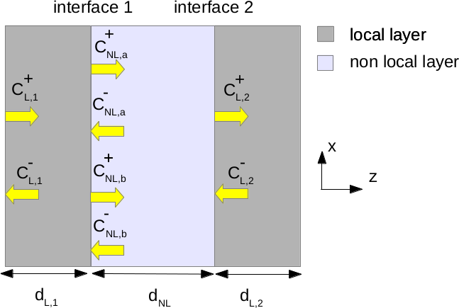
Figure 7: Schematic showing a non-local layer embedded in a local environment.

In this Appendix, the S-matrix for a periodic layer with non-local response, embedded in a local environment is evaluated. The geometry is defined in Fig. 7. Two local layers, labeled as “$L_{1}$” and “$L_{2}$” surround a non-local slab labeled as “NL”. The mode amplitude constants are defined as $C$, with the subscript denoting the layer index, and the superscript the propagation direction, with “+” and “-” standing for waves propagating in the positive and negative z-directions respectively. Each vector of mode amplitudes $C$, has $N$ elements. The non-local layer therefore supports twice as many modes than the local layers, in consistence with the discussion in Section II. For the case that the non-local layer is non-periodic, the solution of Eq. (2) results in $N$ pure transverse and $N$ pure longitudinal modes. Then, the mode amplitude constants can be divided into two groups, $C_{\text{NL,a}}$ and $C_{\text{NL,b}}$ with each of these groups associated with either longitudinal or transverse modes. When the non-local layer is periodic, no pure longitudinal modes exist in the general case. For consistency, we keep the division into two groups $C_{\text{NL,a}}$ and $C_{\text{NL,b}}$ so that each mode amplitude vector remains with $N$ elements. However, the division into these two groups is now arbitrary. To find the mode amplitude vectors, we employ the S-matrix approach, for which a scattering matrix $\mathbf{S}$ relates a vector of incident mode amplitudes $\mathbf{a}$ to a vector of outgoing mode amplitudes $\mathbf{b}$ according to $\mathbf{b}=\mathbf{Sa}$. This approach is considered as numerically stable in the sense that growing exponential terms are avoided lifengli2 . First, the S-matrix for the interfaces are derived and afterwards they are used to derive the layer S-matrix.

The two interface S-matrices are defined as:

$$\left[\begin{array}[]{ccc}S_{11}^{(1)}&S_{12}^{(1)}&S_{13}^{(1)}\\ S_{21}^{(1)}&S_{22}^{(1)}&S_{23}^{(1)}\\ S_{31}^{(1)}&S_{32}^{(1)}&S_{33}^{(1)}\end{array}\right]\left[\begin{array}[]{c}P_{\text{L,1}}^{+}C_{\text{L,1}}^{+}\\ C_{\text{NL,a}}^{-}\\ C_{\text{NL,b}}^{-}\end{array}\right] = \left[\begin{array}[]{c}C_{\text{NL,a}}^{+}\\ C_{\text{NL,b}}^{+}\\ P_{\text{L,1}}^{-}C_{\text{L,1}}^{-}\end{array}\right]$$ (10j)

$$\left[\begin{array}[]{ccc}S_{11}^{(2)}&S_{12}^{(2)}&S_{13}^{(2)}\\ S_{21}^{(2)}&S_{22}^{(2)}&S_{23}^{(2)}\\ S_{31}^{(2)}&S_{32}^{(2)}&S_{33}^{(2)}\end{array}\right]\left[\begin{array}[]{c}C_{\text{L,2}}^{-}\\ P_{\text{NL,a}}^{+}C_{\text{NL,a}}^{+}\\ P_{\text{NL,b}}^{+}C_{\text{NL,b}}^{+}\end{array}\right] = \left[\begin{array}[]{c}P_{\text{NL,a}}^{-}C_{\text{NL,a}}^{-}\\ P_{\text{NL,b}}^{-}C_{\text{NL,b}}^{-}\\ C_{\text{L,2}}^{+}\end{array}\right]$$ (10t)

Here, the phase matrices $P_{\text{L,1}}^{\pm}$ are $N\times N$ diagonal matrices with elements $\exp(jk_{0}k_{z,n}^{(i)\pm}d_{\text{L,1}})$, with $d_{\text{L,1}}$ the local layer thickness as shown in Fig. 7. The forward and backward propagating modes in layer $i$, have propagation constants $k_{z,n}^{(i)+}$ and $k_{z,n}^{(i)-}$ respectively. Since $k_{z,n}^{(i)+}=-k_{z,n}^{(i)-}$, these phase matrices satisfy $P_{\text{L,i}}^{+}=(P_{\text{L,i}}^{-})^{-1}$. For the non-local layer the phase matrices are $P_{\text{NL,x}}^{\pm}$ with x=a,b, with the subscripts and superscripts having their obvious meaning. The phase matrices appear in Eq. (10) because the mode amplitudes are defined to have zero phase at the left boundary of each layer.

Assuming continuity of $E_{x}$, $J_{z}$ and $E_{z}$ we match the eigenvector matrices of these field quantities at the first interface:

$$\left[\begin{array}[]{cc}E_{x,\text{L,1}}^{+}&E_{x,\text{L,1}}^{-}\\ J_{z,\text{L,1}}^{+}&J_{z,\text{L,1}}^{-}\\ E_{z,\text{L,1}}^{+}&E_{z,\text{L,1}}^{-}\end{array}\right]\left[\begin{array}[]{c}P_{\text{L,1}}^{+}C_{\text{L,1}}^{+}\\ P_{\text{L,1}}^{-}C_{\text{L,1}}^{-}\end{array}\right]=\left[\begin{array}[]{cccc}E_{x,\text{NL,a}}^{+}&E_{x,\text{NL,b}}^{+}&E_{x,\text{NL,a}}^{-}&E_{x,\text{NL,b}}^{-}\\ J_{z,\text{NL,a}}^{+}&J_{z,\text{NL,b}}^{+}&J_{z,\text{NL,a}}^{-}&J_{z,\text{NL,b}}^{-}\\ E_{z,\text{NL,a}}^{+}&E_{z,\text{NL,b}}^{+}&E_{z,\text{NL,a}}^{-}&E_{z,\text{NL,b}}^{-}\end{array}\right]\left[\begin{array}[]{c}C_{\text{NL,a}}^{+}\\ C_{\text{NL,b}}^{+}\\ C_{\text{NL,a}}^{-}\\ C_{\text{NL,b}}^{-}\end{array}\right]$$ (11)

Where a “+” or “-” superscript of the eigenvector matrices represents left and right propagating field quantities respectively. Rearranging terms in Eq. (11) we obtain:

$$\left[\begin{array}[]{ccc}E_{x,\text{L,1}}^{+}&-E_{x,\text{NL,a}}^{-}&-E_{x,\text{NL,b}}^{-}\\ J_{z,\text{L,1}}^{+}&-J_{z,\text{NL,a}}^{-}&-J_{z,\text{NL,b}}^{-}\\ E_{z,\text{L,1}}^{+}&-E_{z,\text{NL,a}}^{-}&-E_{z,\text{NL,b}}^{-}\end{array}\right]\left[\begin{array}[]{c}P_{\text{L,1}}^{+}C_{\text{L,1}}^{+}\\ C_{\text{NL,a}}^{-}\\ C_{\text{NL,b}}^{-}\end{array}\right]=\left[\begin{array}[]{ccc}E_{x,\text{NL,a}}^{+}&E_{x,\text{NL,b}}^{+}&-E_{x,\text{L,1}}^{-}\\ J_{z,\text{NL,a}}^{+}&J_{z,\text{NL,b}}^{+}&-J_{z,\text{L,1}}^{-}\\ E_{z,\text{NL,a}}^{+}&E_{z,\text{NL,b}}^{+}&-E_{z,\text{L,1}}^{-}\end{array}\right]\left[\begin{array}[]{c}C_{\text{NL,a}}^{+}\\ C_{\text{NL,b}}^{+}\\ P_{\text{L,1}}^{-}C_{\text{L,1}}^{-}\end{array}\right]$$ (12)

Comparing Eq. (12) with (10j), it is seen that the first interface S-matrix can be expressed by the eigenvector matrices as:

$$\left[\begin{array}[]{ccc}S_{11}^{(1)}&S_{12}^{(1)}&S_{13}^{(1)}\\ S_{21}^{(1)}&S_{22}^{(1)}&S_{23}^{(1)}\\ S_{31}^{(1)}&S_{32}^{(1)}&S_{33}^{(1)}\end{array}\right]=\left[\begin{array}[]{ccc}E_{x,\text{NL,a}}^{+}&E_{x,\text{NL,b}}^{+}&-E_{x,\text{L,1}}^{-}\\ J_{z,\text{NL,a}}^{+}&J_{z,\text{NL,b}}^{+}&-J_{z,\text{L,1}}^{-}\\ E_{z,\text{NL,a}}^{+}&E_{z,\text{NL,b}}^{+}&-E_{z,\text{L,1}}^{-}\end{array}\right]^{-1}\left[\begin{array}[]{ccc}E_{x,\text{L,1}}^{+}&-E_{x,\text{NL,a}}^{-}&-E_{x,\text{NL,b}}^{-}\\ J_{z,\text{L,1}}^{+}&-J_{z,\text{NL,a}}^{-}&-J_{z,\text{NL,b}}^{-}\\ E_{z,\text{L,1}}^{+}&-E_{z,\text{NL,a}}^{-}&-E_{z,\text{NL,b}}^{-}\end{array}\right]$$ (13a)

Following a similar procedure, the second interface S-matrix is:

$$\left[\begin{array}[]{ccc}S_{11}^{(2)}&S_{12}^{(2)}&S_{13}^{(2)}\\ S_{21}^{(2)}&S_{22}^{(2)}&S_{23}^{(2)}\\ S_{31}^{(2)}&S_{32}^{(2)}&S_{33}^{(2)}\end{array}\right]=\left[\begin{array}[]{ccc}E_{x,\text{NL,a}}^{-}&E_{x,\text{NL,b}}^{-}&-E_{x,\text{L,2}}^{+}\\ J_{z,\text{NL,a}}^{-}&J_{z,\text{NL,b}}^{-}&-J_{z,\text{L,2}}^{+}\\ E_{z,\text{NL,a}}^{-}&E_{z,\text{NL,b}}^{-}&-E_{z,\text{L,2}}^{+}\end{array}\right]^{-1}\left[\begin{array}[]{ccc}E_{x,\text{L,2}}^{-}&-E_{x,\text{NL,a}}^{+}&-E_{x,\text{NL,b}}^{+}\\ J_{z,\text{L,2}}^{-}&-J_{z,\text{NL,a}}^{+}&-J_{z,\text{NL,b}}^{+}\\ E_{z,\text{L,2}}^{-}&-E_{z,\text{NL,a}}^{+}&-E_{z,\text{NL,b}}^{+}\end{array}\right]$$ (13b)

By detaching the phase matrices, Eq. (10) can be modified to:

$$\left[\begin{array}[]{ccc}I&0&0\\ 0&I&0\\ 0&0&\left(P_{\text{L,1}}^{-}\right)^{-1}\end{array}\right]\left[\begin{array}[]{ccc}S_{11}^{(1)}&S_{12}^{(1)}&S_{13}^{(1)}\\ S_{21}^{(1)}&S_{22}^{(1)}&S_{23}^{(1)}\\ S_{31}^{(1)}&S_{32}^{(1)}&S_{33}^{(1)}\end{array}\right]\left[\begin{array}[]{ccc}P_{\text{L,1}}^{+}&0&0\\ 0&I&0\\ 0&0&I\end{array}\right]\left[\begin{array}[]{c}C_{\text{L,1}}^{+}\\ C_{\text{NL,a}}^{-}\\ C_{\text{NL,b}}^{-}\end{array}\right]=\left[\begin{array}[]{c}C_{\text{NL,a}}^{+}\\ C_{\text{NL,b}}^{+}\\ C_{\text{L,1}}^{-}\end{array}\right]$$ (14a)

$$\left[\begin{array}[]{ccc}\left(P_{\text{NL,a}}^{-}\right)^{-1}&0&0\\ 0&\left(P_{\text{NL,b}}^{-}\right)^{-1}&0\\ 0&0&I\end{array}\right]\left[\begin{array}[]{ccc}S_{11}^{(2)}&S_{12}^{(2)}&S_{13}^{(2)}\\ S_{21}^{(2)}&S_{22}^{(2)}&S_{23}^{(2)}\\ S_{31}^{(2)}&S_{32}^{(2)}&S_{33}^{(2)}\end{array}\right]\left[\begin{array}[]{ccc}I&0&0\\ 0&P_{\text{NL,a}}^{+}&0\\ 0&0&P_{\text{NL,b}}^{+}\end{array}\right]\left[\begin{array}[]{c}C_{\text{L,2}}^{-}\\ C_{\text{NL,a}}^{+}\\ C_{\text{NL,b}}^{+}\end{array}\right]=\left[\begin{array}[]{c}C_{\text{NL,a}}^{-}\\ C_{\text{NL,b}}^{-}\\ C_{\text{L,2}}^{+}\end{array}\right]$$ (14b)

Preforming the matrix multiplications in Eq. (14) and rearranging terms, we obtain two homogeneous equations:

$$\left[\begin{array}[]{cccccc}S_{11}^{(1)}P_{\text{L,1}}^{+}&S_{12}^{(1)}&S_{13}^{(1)}&-I&0&0\\ S_{21}^{(1)}P_{\text{L,1}}^{+}&S_{22}^{(1)}&S_{23}^{(1)}&0&-I&0\\ P_{\text{L,1}}^{+}S_{31}^{(1)}P_{\text{L,1}}^{+}&P_{\text{L,1}}^{+}S_{32}^{(1)}&P_{\text{L,1}}^{+}S_{33}^{(1)}&0&0&-I\end{array}\right]\left[\begin{array}[]{c}C_{\text{L,1}}^{+}\\ C_{\text{NL,a}}^{+}\\ C_{\text{NL,b}}^{+}\\ C_{\text{NL,a}}^{-}\\ C_{\text{NL,b}}^{-}\\ C_{\text{L,1}}^{-}\end{array}\right]=0$$ (15a)

$$\left[\begin{array}[]{cccccc}P_{\text{NL,a}}^{+}S_{11}^{(2)}&P_{\text{NL,a}}^{+}S_{12}^{(2)}P_{\text{NL,a}}^{+}&P_{\text{NL,a}}^{+}S_{13}^{(2)}P_{\text{NL,b}}^{+}&-I&0&0\\ P_{\text{NL,b}}^{+}S_{21}^{(2)}&P_{\text{NL,b}}^{+}S_{22}^{(2)}P_{\text{NL,a}}^{+}&P_{\text{NL,b}}^{+}S_{23}^{(2)}P_{\text{NL,b}}^{+}&0&-I&0\\ S_{31}^{(2)}&S_{32}^{(2)}P_{\text{NL,a}}^{+}&S_{33}^{(2)}P_{\text{NL,b}}^{+}&0&0&-I\end{array}\right]\left[\begin{array}[]{c}C_{\text{L,2}}^{-}\\ C_{\text{NL,a}}^{+}\\ C_{\text{NL,b}}^{+}\\ C_{\text{NL,a}}^{-}\\ C_{\text{NL,b}}^{-}\\ C_{\text{L,2}}^{+}\end{array}\right]=0$$ (15b)

Combining the two equations in (15), we obtain a system of equations that connect the incident amplitudes ($C_{\text{L,1}}^{+}\text{ and }C_{\text{L,2}}^{-}$) with the outgoing ($C_{\text{L,2}}^{+}\text{ and }C_{\text{L,1}}^{-}$) and internal amplitudes ($C_{\text{NL,a}}^{+},C_{\text{NL,b}}^{+},C_{\text{NL,a}}^{-}\text{ and }C_{\text{NL,b}}^{-}$) :

$$S_{\text{layer}}\left[\begin{array}[]{c}C_{\text{L,1}}^{+}\\ C_{\text{L,2}}^{-}\end{array}\right] = \left[\begin{array}[]{c}C_{\text{L,2}}^{+}\\ C_{\text{L,1}}^{-}\\ C_{\text{NL,a}}^{+}\\ C_{\text{NL,b}}^{+}\\ C_{\text{NL,a}}^{-}\\ C_{\text{NL,b}}^{-}\end{array}\right]$$ (16i)

$$S_{\text{layer}} \equiv A^{-1}B$$ (16j)

$$A \equiv \left[\begin{array}[]{cccccc}0&0&I&0&-S_{12}^{(1)}&-S_{13}^{(1)}\\ 0&0&0&I&-S_{22}^{(1)}&-S_{23}^{(1)}\\ 0&I&0&0&-P_{\text{L,1}}^{+}S_{32}^{(1)}&-P_{\text{L,1}}^{+}S_{33}^{(1)}\\ 0&0&-P_{\text{NL,a}}^{+}S_{12}^{(2)}P_{\text{NL,a}}^{+}&-P_{\text{NL,a}}^{+}S_{13}^{(2)}P_{\text{NL,b}}^{+}&I&0\\ 0&0&-P_{\text{NL,b}}^{+}S_{22}^{(2)}P_{\text{NL,a}}^{+}&-P_{\text{NL,b}}^{+}S_{23}^{(2)}P_{\text{NL,b}}^{+}&0&I\\ I&0&-S_{32}^{(2)}P_{\text{NL,a}}^{+}&-S_{33}^{(2)}P_{\text{NL,b}}^{+}&0&0\end{array}\right]$$ (16q)

$$B \equiv \left[\begin{array}[]{cc}S_{11}^{(1)}P_{\text{L,1}}^{+}&0\\ S_{21}^{(1)}P_{\text{L,1}}^{+}&0\\ P_{\text{L,1}}^{+}S_{31}^{(1)}P_{\text{L,1}}^{+}&0\\ 0&P_{\text{NL,a}}^{+}S_{11}^{(2)}\\ 0&P_{\text{NL,b}}^{+}S_{21}^{(2)}\\ 0&S_{31}^{(2)}\end{array}\right]$$ (16x)

$S_{\text{layer}}$ is a $6N\times 2N$ matrix, which can be divided into two submatrices according to:

$$S_{\text{layer}} \equiv \left[\begin{array}[]{c}S_{\text{external}}\\ S_{\text{internal}}\end{array}\right]$$ (17c)

$$S_{\text{external}} \equiv \left[\begin{array}[]{cc}S_{\text{layer},11}&S_{\text{layer},12}\\ S_{\text{layer},21}&S_{\text{layer},22}\end{array}\right]$$ (17f)

$$S_{\text{internal}} \equiv \left[\begin{array}[]{cc}S_{\text{layer},31}&S_{\text{layer},32}\\ S_{\text{layer},41}&S_{\text{layer},42}\\ S_{\text{layer},51}&S_{\text{layer},52}\\ S_{\text{layer},61}&S_{\text{layer},62}\end{array}\right]$$ (17k)

Eq. (16) and (17) provide a complete description of all mode amplitudes. $S_{\text{external}}$ can be regarded as the ordinary $2N\times 2N$ S-matrix, which couples transverse only modes in the first local layer to transverse only modes in the second local layer. From $S_{\text{internal}}$ the internal (i.e. non-local) amplitudes $C_{\text{NL,a}}^{+},C_{\text{NL,b}}^{+},C_{\text{NL,a}}^{-}\text{ and }C_{\text{NL,b}}^{-}$ can be obtained.

References

• (1) P. J. Feibelman, “Surface electromagnetic fields,” Prog. Surf. Sci. 12, 287–408 (1982).
• (2) A. D. Boardman, Electromagnetic Surface Modes (Wiley, 1982).
• (3) F. Forstmann and R. R. Gerhardts, Metal Optics Near the Plasma Frequency (Springer-Verlag, Berlin, 1986).
• (4) J. M. Pitarke, V. M. Silkin, E. V. Chulkov, and P. M. Echenique, “Theory of surface plasmons and surface-plasmon polaritons,” Rep. Prog. Phys. 70, 1–87 (2007).
• (5) M. Anderegg, B. Feuerbacher, and B. Fitton, “Optically Excited Longitudinal Plasmons in Potassium,” Phys. Rev. Lett. 27, 1565–1568 (1971).
• (6) C. Ciracì, R. T. Hill, J. J. Mock, Y. Urzhumov, A. I. Fernández-Domínguez, S. A. Maier, J. B. Pendry, A. Chilkoti, and D. R. Smith, “Probing the ultimate limits of plasmonic enhancement,” Science 337(6098), 1072–1074 (2012).
• (7) S. Raza, N. Stenger, S. Kadkhodazadeh, S. V. Fischer, N. Kostesha, A.-P. Jauho, A. Burrows, M. Wubs, and N. A. Mortensen, “Blueshift of the surface plasmon resonance in silver nanoparticles studied with EELS,” Nanophotonics 2, 131-138 (2013).
• (8) T. Teperik, P. Nordlander, J. Aizpurua, and A. G. Borisov, “Robust Subnanometric Plasmon Ruler by Rescaling of the Nonlocal Optical Response,” Phys. Rev. Lett. 110, 263901 (2013).
• (9) R. Esteban, A. G. Borisov, P. Nordlander, and J. Aizpurua, “Bridging quantum and classical plasmonics with a quantum-corrected model,” Nature Comm. 3, 825 (2012).
• (10) L. Stella, P. Zhang, F. J. García-Vidal, A. Rubio, and P. García-González, ”Performance of Nonlocal Optics When Applied to Plasmonic Nanostructures,” J. Phys Chem. C 117 (17), 8941-8949 (2013).
• (11) R. Ruppin, “Extinction properties of thin metallic nanowires,” Opt. Commun. 190, 205–209 (2001).
• (12) F. J. García de Abajo, “Nonlocal effects in the plasmons of strongly interacting nanoparticles, dimers, and waveguides,” J. Phys. Chem. C 112, 17983–17987 (2008).
• (13) W. Luis Mochán, Marcelo del Castillo-Mussot, and Rubén G. Barrera, ”Effect of plasma waves on the optical properties of metal-insulator superlattices,“ Phys. Rev. B 35, 1088-1098 (1987).
• (14) V. Yannopapas, “Non-local optical response of two-dimensional arrays of metallic nanoparticles,” J. Phys. Condens. Matt. 20, 325211 (2008).
• (15) S. Raza, G. Toscano, A.-P. Jauho, M. Wubs and N. A. Mortensen, “Unusual resonances in nanoplasmonic struc- tures due to nonlocal response,” Phys. Rev. B 84, 121412(R) (2011).
• (16) A. I. Fernández-Domínguez, A. Wiener, F. J. García-Vidal, S. A. Maier, and J. B. Pendry, “Transformation-optics description of nonlocal effects in plasmonic nanostructures,” Phys. Rev. Lett. 108, 106802 (2012).
• (17) G. Toscano, S. Raza, A.-P. Jauho, N. A. Mortensen, and M. Wubs, “Modified field enhancement and extinction by plasmonic nanowire dimers due to nonlocal response,” Opt. Express 20, 4176-4188 (2012).
• (18) G. Toscano, S. Raza, W. Yan, C. Jeppesen, S. Xiao, M. Wubs, A.-P. Jauho, S.I. Bozhevolnyi and N.A. Mortensen, “Nonlocal response in plasmonic waveguiding with extreme light confinement,” Nanophotonics 2(3), 161-166 (2013).
• (19) K. R. Hiremath, L. Zschiedrich, and F. Schmidt, “Numerical solution of nonlocal hydrodynamic Drude model for arbitrary shaped nano-plasmonic structures using Nédélec finite elements,” J. Comput. Phys. 231(17), 5890–5896 (2012).
• (20) M. G. Moharam, E. B. Grann, D. A. Pommet, and T. K. Gaylord, “Formulation for stable and efficient implementation of the rigorous coupled-wave analysis of binary gratings,” J. Opt. Soc. Am. A 12, 1068–1076 (1995).
• (21) P. Lalanne and G. Morris, “Highly improved convergence of the coupled-wave method for TM polarization,” J. Opt. Soc. Am. A 13, 779–784 (1996).
• (22) L. Li, “Formulation and comparison of two recursive matrix algorithms for modeling layered diffraction gratings,” J. Opt. Soc. Am. A 13, 1024–1035 (1996).
• (23) H. Liu and P. Lalanne, “Microscopic theory of the extraordinary optical transmission,” Nature 452(7188), 728–731 (2008).
• (24) A. D. Boardman and R. Ruppin, “The boundary conditions between spatially dispersive media,” Surf. Sci. 112, 153 (1981).
• (25) A. R. Melnyk and M. J. Harrison, “Theory of optical excitation of plasmons in metals,” Phys. Rev. B 2(4), 835–850 (1970).
• (26) W. Yan, M. Wubs, and N. A. Mortensen, “Hyperbolic meta- materials: nonlocal response regularizes broadband super-singularity,” Phys. Rev. B 86, 205429 (2012).
• (27) A. Moreau, C. Ciracì and D. Smith, “Impact of nonlocal response on metallodielectric multilayers and optical patch antennas,” Phys. Rev. B 87,045401 (2013).
• (28) S. Shi, C. Chen, and D.W. Prather, “Revised plane wave method for dispersive material and its application to band structure calculations of photonic crystal slabs,” Appl. Phys. Lett. 86, 043104 (2005).
• (29) J. D. Joannopoulos, S. G. Johnson, J. N. Winn, and R. D. Meade, Photonic Crystals: Molding the Flow of Light, 2nd ed. (Princeton University Press, 2008).
• (30) A. Raman and S. Fan, “Photonic band structure of dispersive metamaterials formulated as a Hermitian eigenvalue problem,” Phys. Rev. Lett. 087401 (2010).
• (31) See http://www.cs.huji.ac.il/$\sim$ulevy/movies/supplemental.gif for an animation, showing $\nabla\cdot J$ at the same frequencies as those in Fig. 3. This animation manifests visually Fig. 2, namely, the phase accumulation in the z-direction is apparent for the absorption peaks.
• (32) M. G. Blaber, M. D. Arnold, and M. J. Ford, ”Search for the Ideal Plasmonic Nanoshell: The Effects of Surface Scattering and Alternatives to Gold and Silver ,” J. Phys. Chem. C 113, 3041 (2009).
• (33) L. Li, “Use of Fourier series in the analysis of discontinuous periodic structures,” J. Opt. Soc. Am. A 13, 1870-1876 (1996).
• (34) J. G. Pedersen, S. Xiao, and N. A. Mortensen, “Limits of slow light in photonic crystals,” Phys. Rev. B 78, 153101 (2008).
• (35) N. Engheta, “Circuits with light at nanoscales: optical nanocircuits inspired by metamaterials,” Science 317(5845), 1698–1702 (2007).