Effect of quantum dot shape of the GaAs/AlAs heterostructure on interlevel hole light absorption

Abstract

The effect of quantum dot shape on the hole energy spectrum and optical properties caused by the interlevel charge transition based on the $4\times 4$ Hamiltonian has been studied for the GaAs quantum dot in the AlAs semiconductor matrix. Calculations have been carried out in perturbation theory taking into account the hybridization of states for cubic, ellipsoidal, cylindrical and tetrahedral shapes by changing the volume of a quantum dot. Based on the energy calculations and on the determined wave functions of the hole states we have defined the selection rules and the dependence of the interlevel hole absorption coefficient on QD shapes and volumes.

Key words: multiband approximation, optical transitions, oscillator strength, absorption coefficient

PACS: 71.15.-m, 78.20.Ci, 78.67.Hc

Abstract

Для квантової точки GaAs у напiвпровiдниковiй матрицi AlAs дослiджено вплив форми квантової точки на енергетичний спектр дiрки та оптичнi властивостi, зумовленi мiжрiвневими переходами заряду, на основi гамiльтонiана $4\times 4$. Обчислення проводились за допомогою теорiї збурень з врахуванням гiбридизацiї станiв для кубiчної, елiпсоїдальної, цилiндричної та тетраедричної форми при змiнi об’єму квантової точки. На основi проведених обчислень енергiї та визначених хвильових функцiй станiв дiрки встановлено правила вiдбору та дослiджено залежнiсть коефiцiєнту мiжрiвневого дiркового поглинання свiтла вiд форми та об’єму квантової точки.

Ключовi слова: багатозонне наближення, оптичнi переходи, сили осцилятора, коефiцiєнт поглинання

Introduction

Lately, quantum dots (QDs) have attracted the attention of researchers both as an object of the study of nanoheterostructure physical properties and as an opportunity for different applications of QDs in everyday life.

As concerns the practical use, QDs are used not only in solar batteries, where the shape and size of CdSe/TiO₂ QDs make it possible to improve the photoresponse [1], but also for the comparison with organic dyes as fluorescent labels based on luminescence and fluorescence [2].

Nowadays, various fields of science use the achievements of physics of nanosize heterostructures, quantum dots in particular. QDs are actively used in the advanced medical technology and cytology [3]. The effect of QD shape is of great importance in these processes. The recent researches show that the shape of quantum dots affects CdTe quantum dot phagocytosis [4].

As noted above, the shape has a significant effect on the QD physical properties. For example, the authors of [5] proved that the shape of a quantum dot affects not only the energy of charges in QDs, but also their electronic density of states. The effect of the shape on the piezoelectric effect and electronic properties of In(Ga)As/GaAs quantum dots, as well as on the longitudinal photoconductivity of multilayer Ge/Si structures with Ge quantum dots has also been visibly demonstrated [6, 7].

Recent experimental investigations reveal the effect of QD shape on the structure and arrangement of Si/Ge quantum dots in the arrays that are used in nanoelectrical devices [8]. The role of QD shape is determinant in obtaining various shapes and sizes of a QD by precipitation [9].

The goal of modern theoretical research is to bring the results to the best agreement with experimental data. Therefore, while calculating physical parameters of semiconductor nanoheterostructures, one should take into account a real band crystal structure of the nanosystem [10, 11].

Applying the envelope-function approximation to the description of hole states in QDs embedded in a semiconductor matrix, we can find not only the energy spectrum and wave functions of particles, but also examine the optical effects caused by interlevel hole transitions [12, 13]. It is known that the optical selection rules, oscillator strength, and interlevel hole absorption coefficient essentially depend on the QD size and shape [14, 15, 16].

The aim of the present work is to study the effect of QD shape on the hole energy spectrum and on the optical parameters (the hole transition probability, transition oscillator strength, interband light absorption coefficient) of a semiconductor nanoheterosystem. QDs of wide energy-band gap semiconductors have been considered and exact solutions of the Schrödinger equation for a hole in a spherical QD in the four-band effective-mass approximation have been used. QDs of other shapes (cubic, ellipsoidal, cylindrical, tetrahedral) have been chosen to be of the same volume and in such a way that the potential energy of carriers for the QD shape of interest should be close to its potential energy in a spherical QD. The calculations have been carried out for the GaAs QD which is placed into the AlAs matrix.

1 The energy and wave functions of bound states of holes in a QD

We study a semiconductor QD embedded in a semiconductor or dielectric matrix with a larger energy gap. If the QD has a spherical shape, for many semiconductor systems the problem of finding the hole energy spectrum (under certain assumptions) is solved analytically.

We consider such crystals of a heterostructure in which the Brillouin zone center is a point of the valence band degeneracy. This valence band structure is observed in most semiconductors. Let us consider the semiconductor heterostructures in which the spin-orbit interaction does not significantly affect the basic hole properties. This can be done if the parameter of this interaction is sufficiently large. Then, the spin-orbit band can be neglected.

Ignoring the warping of the isoenergetic surfaces in the $k$-space (spherical approximation), the hole Hamiltonian can be presented as [17]

$$\hat{H}_{0}=\frac{1}{2}\left(\gamma_{1}+\frac{5}{2}\gamma\right)\hat{p}^{2}-\gamma\left(\hat{\vec{p}}\cdot\hat{\vec{J}}\right)^{2}+U_{\textrm{s}}\left(r\right),$$ (1)

where $\gamma,\gamma_{1},\,\,\gamma_{2},\,\,\gamma_{3}$ are the Luttinger parameters [where $\gamma=1/5\left(3\gamma_{3}+2\gamma_{2}\right)$], $\hat{\vec{J}}$ is the spin momentum operator, for which $J^{2}=\hbar^{2}j(j+1),$ $j=3/2$, $\hat{\vec{p}}$ is the quasiparticle momentum operator, $U_{\textrm{s}}\left(r\right)$ is the charge potential energy in a spherical QD.

The wave function, which is a solution of the equation with the Hamiltonian (1), is expressed as a product of the total momentum operator eigenfunctions and radial functions [18]. As shown in [17, 19], it is convenient to divide the solutions obtained with this wave function into even and odd states, (I, II). Taking into account the states with $f=3/2,5/2$, we choose them as follows:

$$v_{f,L,M}\left(r,\theta,\phi\right)=\left\{\begin{array}[]{ll}{v_{f,L,M}^{\textrm{I}}\left(r,\theta,\phi\right)=R_{2}^{\textrm{I}}\left(r\right)\Phi_{f,M}^{f-\frac{3}{2}}\left(\theta,\phi\right)+R_{1}^{\textrm{I}}\left(r\right)\Phi_{f,M}^{f+\frac{1}{2}}\left(\theta,\phi\right),}&{\left(L=f-\frac{3}{2},f+\frac{1}{2}\right),}\\[4.30554pt] {v_{f,L,M}^{\textrm{II}}\left(r,\theta,\phi\right)=R_{2}^{\textrm{II}}\left(r\right){\Phi_{f,M}^{f-\frac{1}{2}}\left(\theta,\phi\right)}+R_{1}^{\textrm{II}}\left(r\right)\Phi_{f,M}^{f+\frac{3}{2}}\left(\theta,\phi\right),}&{\left(L=f-\frac{1}{2},f+\frac{3}{2}\right),}\end{array}\right.$$ (2)

where $\Phi_{f,M}^{L}\left(\theta,\phi\right)$ are the four-component spinors corresponding to spin $j=3/2$. A general form of spinors can be also represented in terms of the Clebsch-Jordan coefficients [20]

$$\Phi_{f,M}^{L}\left(\theta,\phi\right)=\sum_{m=-L}^{L}\sum_{m_{j}=-j}^{j}G_{L,m;j,m_{j}}^{f,M}Y_{L,m}\left(\theta,\phi\right)\xi_{m_{j}}\,.$$ (3)

where $Y_{L,m}$ are spherical harmonics, $\xi_{m_{j}}$ is the spinor function.

In the inner region of the heterosystem ($r\leqslant a$), the solutions of the corresponding equations can be written using the Bessel functions of the first kind

$$R_{1}^{i,(1)}\left(r\right) = \frac{{B_{1}^{(1)}}}{{\sqrt{r}}}{J_{L+\frac{5}{2}}}\left({\frac{{{k^{(1)}}r}}{{\sqrt{1-{{\left({{\mu^{(1)}}}\right)}^{2}}}}}}\right)+\frac{{B_{2}^{(1)}}}{{\sqrt{r}}}{J_{L+\frac{5}{2}}}\left({\frac{{{k^{(1)}}r}}{{\sqrt{1+{{\left({{\mu^{(1)}}}\right)}^{2}}}}}}\right),$$

$$R_{2}^{i,(1)}\left(r\right) = \frac{B_{1}^{(1)}\left(C_{1}^{(1)}-\mu^{(1)}\right)}{\sqrt{r}\sqrt{\left(\mu^{(1)}\right)^{2}-\left(C_{1}^{(1)}\right)^{2}}}{J}_{L+\frac{1}{2}}\left(\frac{k^{(1)}r}{\sqrt{1-\left(\mu^{(1)}\right)^{2}}}\right)$$ (4)

$${+\frac{B_{2}^{(1)}\left(C_{1}^{(1)}+\mu^{(1)}\right)}{\sqrt{r}\sqrt{\left(\mu^{(1)}\right)^{2}-\left(C_{1}^{(1)}\right)^{2}}}{J}_{L+\frac{1}{2}}\left(\frac{k^{(1)}r}{\sqrt{1+\left(\mu^{(1)}\right)^{2}}}\right),}$$

where

$$k^{(1)}=\sqrt{2E/\gamma_{1}^{(1)}},\qquad\lambda^{(1)}=\sqrt{2E/\left[\gamma_{1}^{(1)}\left(1+\mu^{(1)}\right)\right]},\qquad\mu^{(1)}=\frac{2\gamma^{(1)}}{\gamma_{1}^{(1)}},\qquad i=\textrm{I,\,II}.$$

In the matrix for $r>a$, the solutions of the equations can be represented by modified Bessel functions of the second kind

$$R_{1}^{i,(2)}\left(r\right) = \frac{D_{1}^{(2)}}{\sqrt{r}}K_{L+\frac{5}{2}}\left(\frac{k^{(2)}r}{\sqrt{1-\left(\mu^{(2)}\right)^{2}}}\right)+\frac{D_{2}^{(2)}}{\sqrt{r}}K_{L+\frac{5}{2}}\left(\frac{k^{(2)}r}{\sqrt{1+\left(\mu^{(2)}\right)^{2}}}\right),$$

$$R_{2}^{i,(2)}\left(r\right) = \frac{D_{1}^{(2)}\left(-C_{1}^{(2)}+\mu^{(2)}\right)}{\sqrt{r}\sqrt{\left(\mu^{(2)}\right)^{2}-\left(C_{1}^{(2)}\right)^{2}}}K_{L+\frac{1}{2}}\left(\frac{k^{(2)}r}{\sqrt{1-\left(\mu^{(2)}\right)^{2}}}\right)$$ (5)

$$+\frac{D_{2}^{(2)}\left(-C_{1}^{(2)}-\mu^{(2)}\right)}{\sqrt{r}\sqrt{\left(\mu^{(2)}\right)^{2}-\left(C_{1}^{(2)}\right)^{2}}}K_{L+\frac{1}{2}}\left(\frac{k^{(2)}r}{\sqrt{1+\left(\mu^{(2)}\right)^{2}}}\right),$$

where

$$k^{(2)}=\sqrt{2\left(U_{0}-E\right)/\gamma_{1}^{(2)}},\qquad\lambda^{(2)}=\sqrt{2\left(U_{0}-E\right)/\left[\gamma_{1}^{(2)}\left(1+\mu^{(2)}\right)\right]},\qquad\mu^{(2)}=\frac{2\gamma^{(2)}}{\gamma_{1}^{(2)}},\qquad i=\textrm{I,\,II}.$$

In order to match the solutions, two conditions have been used: the continuity of the radial wave function and the normal component of the probability density flux through a QD spherical surface [21]. Under such conditions one can define the wave functions of the hole states $v_{fLMn}$ ($n=1,\,2,\,3,\,\dots$ is the ordinal number of solution of the dispersion equation) and the energies for different values of the radius (volume) of the spherical QD. We will consider further QDs of cubic, ellipsoidal, cylindrical and pyramidal shapes having the volume identical with that of a spherical QD. In this case the potential $U(\vec{r})$ for a hole of the QD of any shape is not significantly different from the potential $U_{\textrm{s}}(r)$ of the charge in a spherical QD as is shown by calculations. Then, the Schrödinger equation can be presented in the form

$$\left[\frac{1}{2}\left(\gamma_{1}+\frac{5}{2}\gamma\right)\hat{p}^{2}-\gamma\left(\hat{\vec{p}}\cdot\hat{\vec{J}}\right)^{2}+U_{\textrm{s}}\left(r\right)+W(\vec{r})\right]\psi(\vec{r})=E\psi(\vec{r}),$$ (6)

where $W(\vec{r})=U(\vec{r})-U_{\textrm{s}}(r)$ is the perturbation potential. The potential $W(\vec{r})$ has the symmetry of the considered QD, which is lower than the symmetry of a spherical QD.

Let us investigate the genesis of the hole quantum states by changing the QD shape. To achieve this aim, we introduce the wave function $\psi$ as a linear combination of functions $v_{fLMn}$ (2) and find the energy spectrum of holes in real QD:

$$\psi=\sum_{fLMn}C_{fLMn}\,v_{fLMn}\,.$$ (7)

Equation (6) can be represented by a set of linear algebraic equations

$$\sum_{f^{\prime}L^{\prime}M^{\prime}n^{\prime}}\langle fLMn|\hat{H}|f^{\prime}L^{\prime}M^{\prime}n^{\prime}\rangle C_{f^{\prime}L^{\prime}M^{\prime}n^{\prime}}=E\;C_{fLMn}\,,$$ (8)

where $\langle fLMn|\hat{H}|f^{\prime}L^{\prime}M^{\prime}n^{\prime}\rangle=\varepsilon_{fLMn}\delta_{f,f^{\prime}}\delta_{L,L^{\prime}}\delta_{M,M^{\prime}}\delta_{n,n^{\prime}}+W_{fLMn,f^{\prime}L^{\prime}M^{\prime}n^{\prime}}$, $\varepsilon_{fLMn}$ is the corresponding energy of a spherical QD.

The diagonalization of the $\langle fLMn|\hat{H}|f^{\prime}L^{\prime}M^{\prime}n^{\prime}\rangle$ matrix applying a unitary transformation is required to find the hole spectrum

$$\sum_{\begin{smallmatrix}{l}{f^{\prime}L^{\prime}M^{\prime}n^{\prime}}\\ {f^{\prime\prime}L^{\prime\prime}M^{\prime\prime}n^{\prime\prime}}\end{smallmatrix}}\langle fLMn|U\hat{H}U^{-1}|f^{\prime\prime}L^{\prime\prime}M^{\prime\prime}n^{\prime\prime}\rangle U_{f^{\prime\prime}L^{\prime\prime}M^{\prime\prime}n^{\prime\prime},f^{\prime}L^{\prime}M^{\prime}n^{\prime}}C_{f^{\prime}L^{\prime}M^{\prime}n^{\prime}}=$$

$$\qquad\qquad\qquad=E\,\sum_{f^{\prime}L^{\prime}M^{\prime}n^{\prime}}U_{fLMn,f^{\prime}L^{\prime}M^{\prime}n^{\prime}}C_{f^{\prime}L^{\prime}M^{\prime}n^{\prime}}\;.$$ (9)

We get

$$\sum_{f^{\prime}L^{\prime}M^{\prime}n^{\prime}}\left(\hat{H}_{fLMn,f^{\prime}L^{\prime}M^{\prime}n^{\prime}}\delta_{f,f^{\prime}}\delta_{L,L^{\prime}}\delta_{M,M^{\prime}}\delta_{n,n^{\prime}}-E\right)\tilde{C}_{f^{\prime}L^{\prime}M^{\prime}n^{\prime}}=0\,,$$ (10)

where $\hat{H}=U\hat{H}U^{-1}$ and $\tilde{C}_{f^{\prime}L^{\prime}M^{\prime}n^{\prime}}=\;\sum_{f^{\prime}L^{\prime}M^{\prime}n^{\prime}}U_{fLMn,f^{\prime}L^{\prime}M^{\prime}n^{\prime}}C_{f^{\prime}L^{\prime}M^{\prime}n^{\prime}}$.

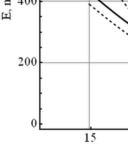
Figure 1: The hole energy of a cubic QD.

Further on, we will consider in more detail the change of the hole energy for the three lowest levels in a spherical QD (dashed lines in figures 1–4) and in QDs of lower symmetry shape (solid lines). In the sum (7) we restrict ourselves to the wave functions of the first three levels of the spherical QD. Then, we have 14 different wave functions (2) and coefficients $\tilde{C}_{f^{\prime}L^{\prime}M^{\prime}n^{\prime}}$ , and the $\langle fLMn|\hat{H}|f^{\prime}L^{\prime}M^{\prime}n^{\prime}\rangle$ matrix contains 196 elements.

The calculations have been performed for the GaAs/AlAs heterosystem (GaAs: $\gamma=7.1$, $\gamma_{1}~{}=~{}2.554$; AlAs: $\gamma=3.76$, $\gamma_{1}=1.212$; $U_{0}=1.071$ eV — band offset). We have found the energy of the ground and excited states for the cubic, ellipsoidal, cylindrical, and pyramidal GaAs QD as a function of its volume. We note that the volume of a spherical QD, $\frac{4}{3}\pi R^{3}$, is equal to the volume of the other QDs.

In figures 1–4, dashed lines indicate the energy of the first three hole levels with quantum numbers $f=3/2$, $L=0$, $n=1$; $f=3/2$, $L=1$, $n=1$; $f=5/2$, $L=1$, $n=1$. The hole energy spectrum transforms in the cubic QD (figure 1). In this case, the energies of the first two levels (solid lines 1, 2) are larger than the energies of the similar levels in the spherical QD. Solid lines 3 and 4 correspond to two- and fourfold degenerate levels obtained by splitting the second excited hole energy level of the spherical QD. Further, we consider the states with $n=1$ only, so this quantum number is omitted in the expressions of wave functions.

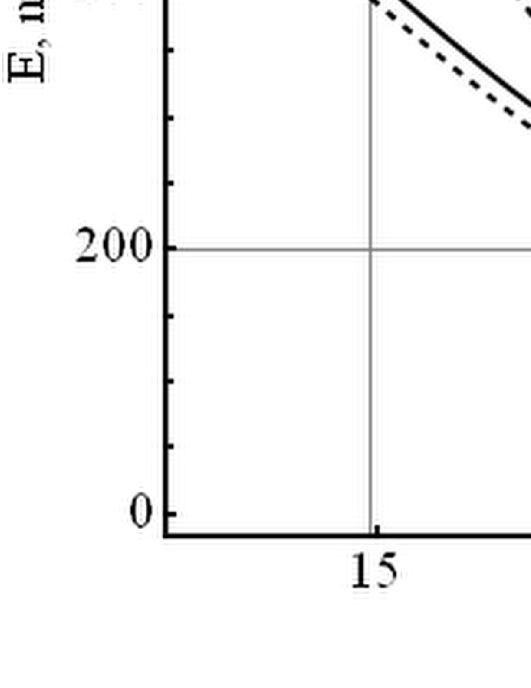
Figure 2: The hole energy of an ellipsoidal QD.

In figure 2 solid lines 1–3 correspond to the energy of the three first levels of holes in the ellipsoidal QD. As seen from the figure, changing the shape from a spherical to an ellipsoidal one is not followed by splitting any levels.

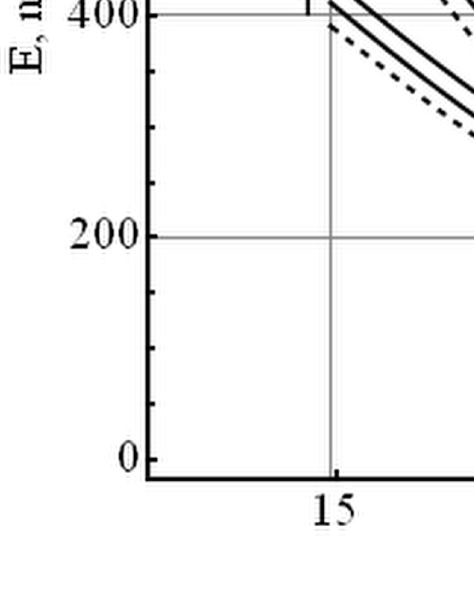
Figure 3: The hole energy of a cylindrical QD.

In a cylindrical QD (figure 3), characterized by axial symmetry, three levels of the spherical QD (dashed lines) correspond to six energy levels (solid lines). In figure 3, lines 1 and 2 indicate the energies of double degenerate levels corresponding to the ground state of the spherical QD, 3 and 4 denote the energies of double degenerate excited levels, lines 5 and 6 indicate the energies, respectively, of four- and twofold degenerate ones.

The calculations show that the hole energy spectrum in a tetrahedron-shaped QD differs from the hole spectrum of a spherical QD (figure 4) more than in the case of the above mentioned shapes. Like in the previous figures, dashed lines represent the first three energy states of a spherical QD and solid lines denote the energy states obtained in a tetrahedral QD after splitting.

It is seen from the figures that for a QD of any form, the energies of all levels decrease with increasing the QD volume. Also, we see that for all shapes of QDs in the considered size limit, the corresponding energy levels are higher than those in a spherical QD. This result can be explained by stronger confinement of charges in the QDs of interest than in the spherical QD.

The wave functions of the hole states are much different even qualitatively in these types of QDs. For example, in a cubic QD at $V=34$ nm³, the wave functions of the states with different energies are written as

$$E_{1}\;-\;\Psi_{1} =v_{\frac{3}{2},0,\frac{3}{2}}\,,$$

$$\quad\quad\Psi_{2} =v_{\frac{3}{2},0,-\frac{3}{2}}\,,$$

$$\quad\quad\Psi_{3} =v_{\frac{3}{2},0,-\frac{1}{2}}\,,$$

$$\quad\quad\Psi_{4} =v_{\frac{3}{2},0,\frac{1}{2}}\,,$$

$$E_{2}\;-\;\Psi_{5} =-0.99v_{\frac{3}{2},1,\frac{3}{2}}-0.15v_{\frac{5}{2},1,-\frac{5}{2}}-0.08v_{\frac{5}{2},1,\frac{3}{2}}\,,$$

$$\quad\quad\Psi_{6} =-0.99v_{\frac{3}{2},1,-\frac{3}{2}}+0.08v_{\frac{5}{2},1,-\frac{3}{2}}+0.15v_{\frac{5}{2},1,\frac{5}{2}}\,,$$

$$\quad\quad\Psi_{7} =0.98v_{\frac{3}{2},1,-\frac{1}{2}}-0.11v_{\frac{3}{2},1,\frac{1}{2}}+0.14v_{\frac{5}{2},1,-\frac{1}{2}}+0.02v_{\frac{5}{2},1,\frac{1}{2}}\,,$$

$$\quad\quad\Psi_{8} =0.11v_{\frac{3}{2},1,-\frac{1}{2}}+0.98v_{\frac{3}{2},1,\frac{1}{2}}+0.02v_{\frac{5}{2},1,-\frac{1}{2}}-0.14v_{\frac{5}{2},1,\frac{1}{2}}\,,$$

$$E_{3}\;-\;\Psi_{9} =0.07v_{\frac{3}{2},1,-\frac{3}{2}}+0.99v_{\frac{5}{2},1,-\frac{3}{2}}-0.05v_{\frac{5}{2},1,\frac{5}{2}}\,,$$

$$\quad\quad\Psi_{10} =-0.07v_{\frac{3}{2},1,\frac{3}{2}}-0.05v_{\frac{5}{2},1,-\frac{5}{2}}+0.99v_{\frac{5}{2},1,\frac{3}{2}}\,,$$

$$E_{4}\;-\;\Psi_{11} =0.15v_{\frac{3}{2},1,-\frac{3}{2}}+0.04v_{\frac{5}{2},1,-\frac{3}{2}}+0.99v_{\frac{5}{2},1,\frac{5}{2}}\,,$$

$$\quad\quad\Psi_{12} =0.15v_{\frac{3}{2},1,\frac{3}{2}}-0.99v_{\frac{5}{2},1,-\frac{5}{2}}-0.04v_{\frac{5}{2},1,\frac{3}{2}}\,,$$

$$\quad\quad\Psi_{13} =-0.1v_{\frac{3}{2},1,-\frac{1}{2}}+0.1v_{\frac{3}{2},1,\frac{1}{2}}+0.7v_{\frac{5}{2},1,-\frac{1}{2}}+0.7v_{\frac{5}{2},1,\frac{1}{2}}\,,$$

$$\quad\quad\Psi_{14} =-0.1v_{\frac{3}{2},1,-\frac{1}{2}}-0.1v_{\frac{3}{2},1,\frac{1}{2}}+0.7v_{\frac{5}{2},1,-\frac{1}{2}}-0.7v_{\frac{5}{2},1,\frac{1}{2}}\,.$$

The calculations make it possible to obtain the wave functions of the states for all the considered shapes and volumes of QDs.

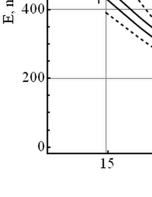
Figure 4: The hole energy of a pyramidal QD.

2 The interlevel absorption coefficient

We consider the case when linearly polarized light falls on the QD along the z-axis which coincides with the axis of symmetry of the QD. Then, the dipole momentum of transition between the $i\alpha$ and $j\beta$ states can be presented as

$$M_{i\alpha,j\beta}=\left\langle j\beta\left|ez\right|i\alpha\right\rangle=\int\Psi_{j\beta}^{*}(x,y,z)\ ez\ \Psi_{i\alpha}(x,y,z)\mathrm{d}V,$$ (11)

and the transition oscillator strength is written as

$$f_{i\alpha,j\beta}=\frac{2m_{0}}{e^{2}\hbar^{2}}(E_{j}-E_{i})\left|M_{ia,j\beta}\right|^{2}.$$ (12)

The light absorption coefficient caused by the hole interlevel transition from the $E_{i}$ level into another energy level $E_{j}$ is defined as

$$\alpha\left(\omega\right)=\omega\sqrt{\frac{\mu_{0}}{\varepsilon_{0}\varepsilon}}\sum_{i,j}\sum_{\alpha,\beta}\frac{\sigma\left|M_{i\alpha,j\beta}\right|^{2}\hbar\Gamma_{i\alpha,j\beta}}{(E_{j}-E_{i}-\hbar\omega)^{2}+\left(\hbar\Gamma_{i\alpha,j\beta}\right)^{2}}\,,$$ (13)

where $\alpha=1,2,\ldots,s_{\alpha}$, $\beta=1,2,\ldots,s_{\beta}$, $s_{\alpha}$ is the multiplicity of the degenerate level $i$, $s_{\beta}$ is the multiplicity of the degenerate level $j$, $\omega$ is the frequency of electromagnetic wave, $\varepsilon_{0}$ is the vacuum permittivity, $\mu_{0}$ is the vacuum permeability, $\varepsilon$ is the relative permittivity of a QD, $\hbar\Gamma_{i\alpha,j\beta}$ is the relaxation energy due to the electron-phonon interaction and other scattering factors. The QD charge density $\sigma$ is chosen on the assumption that there can be only one electron in a QD, so $\sigma=3/\left(4\pi a^{3}\right)$.

According to the above formulas, we calculate the probability of optical transitions, the transition oscillator strength, and the light absorption coefficient for different geometric shapes of a QD. These physical quantities are compared with the corresponding parameters of the spherical-symmetry QD, for which transitions are allowed only between the levels under the following conditions:

• transitions between states of equal parity are possible if $f^{\prime}-f=\pm 1$, $M^{\prime}-M=0,\pm 1$;

• transitions between odd and even states are possible if $f^{\prime}-f=0$, $M^{\prime}-M=0,\pm 1$.

Equation (13) allows one to determine the dependence of the absorption coefficient on the frequency of external electromagnetic wave for transitions of the charge between the lowest levels for all the QD shapes. In figure 5 we present the dependence $\alpha=\alpha(\omega)$ at $V=34nm^{3}$. Dashed lines correspond to the function $\alpha(\omega)$ for a spherical QD.

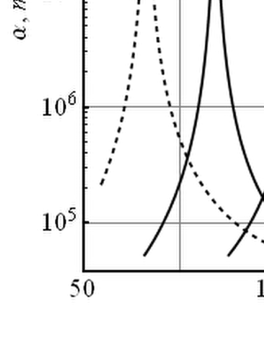
Figure 5: Absorption coefficients of interlevel optical transitions in a cubic (2) and a pyramidal (3) QDs in logarithmic scale. Dashed lines (1) correspond to a spherical QD.

It is obvious that for spherical [figure 5, (1)] and cubic [figure 5, (2)] QD shapes, not only the absorption maxima differ, but also their energy, which is due to the difference between electron transition energies at a given size of the QD. So, if the absorption maximum for the two lowest levels in a spherical QD is equal to $8\cdot 10^{7}$ m^-1 with the energy 65 meV, then the cubic QD value of the corresponding interlevel absorption coefficient is $4.8\cdot 10^{7}$ m^-1 with the energy 85 meV, i.e., in a cubic QD the absorption maximum shifts towards higher energies with respect to a spherical QD. The absolute value of the maximum absorption coefficient between the second and the third lowest levels is lower (respectively, $5.6\cdot 10^{7}$ m^-1 and $1.5\cdot 10^{7}$ m^-1 for the sphere and cube). Besides, in the cubic QD, one observes the absorption peak shift towards lower energies. As to the third absorption band, which is caused by hole transitions between the first and third hole lowest levels, the maximum $\alpha(\omega)$ is the largest for all QD shapes (about $1.2\cdot 10^{9}$ m^-1).

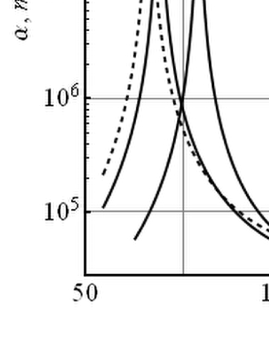
Figure 6: Absorption coefficients of interlevel optical transitions in an ellipsoidal (2) and a cylindrical (3) QDs in logarithmic scale.

Comparing the absorption rate for interlevel optical transitions in QDs of ellipsoidal and spherical shapes [figure 6, (2)], we can see that the maxima of the absorption coefficient are almost the same ($6.4\cdot 10^{7}$ $m^{-1}$, $8\cdot 10^{7}$ $m^{-1}$) for a transition of the charge between the two first levels, and the energies almost coincide (respectively, 70 and 65 meV). A small difference between these physical parameters of QDs can be explained by similarity of shapes between the sphere and the ellipsoid. It should be noted that all the maxima of the interlevel absorption coefficient in the ellipsoidal QD are shifted towards higher energies in comparison with the spherical QD.

As concerns the QD of cylindrical shape [figure 6, (3)], the maxima of the light absorption coefficient in the hole transitions between the first and the second, or between the second and the third lowest energy levels are close to the respective maxima of the spherical QD ($4\cdot 10^{7}$ m^-1 and $3.1\cdot 10^{7}$ m^-1). The energies at which absorption occurs in the cylindrical QD (80 and 165 meV) are also close to the corresponding energies of the spherical QD (65 and 170 meV).

The QD of a regular tetrahedron shape differs greatly from the shape of the sphere. Therefore, the absorption coefficient of hole interlevel transitions in these QDs is also different [Fig. 5, (2)]. The maxima $\alpha(\omega)$ for the charge transition between the three lowest levels are different from the maxima of the spherical QD (105 and 145 meV for a tetrahedral QD, 65 and 170 meV for a spherical QD). The absorption peaks are shifted towards larger and smaller energies, respectively, in comparison with the absorption peaks of a spherical QD.

The performed calculations based on the measurements $\alpha=\alpha(\omega)$, allow one to establish the shape of a QD which, as one can see, has a significant impact on the optical properties of a heterostructure.

3 Conclusions

The effect of the shape on the hole energy spectrum of a GaAs/AlAs heterostructure was investigated in this work. One takes into account the valence band degeneracy of two adjacent materials at a $\Gamma$ point of the Brillouin zone. The problem is solved for spherical, cubic, ellipsoidal (spheroidal), cylindrical, and pyramidal QDs provided their volumes are the same.

There are two types of QDs in our investigation. Some of them (spherical, cubic, pyramidal QDs) are characterized by one size parameter (radius or length of the edge). This parameter determines the volume of the QD. The volume of the other QDs is determined by means of two characteristic linear dimensions. Particularly, a QD of spheroidal shape is characterized by the length of small ($a$) and major ($b$) semiaxes, and a cylindrical QD is characterized by height ($h$) and diameter ($d$). The analysis shows that the potential $W$ (6) can be considered as small perturbation for $15~{}\text{nm}^{3}\leqslant V\leqslant 530~{}\text{nm}^{3}$ if ratios $b/a\leqslant 1.5$; $h/d\leqslant 1.25$. These ratios of a spheroidal and cylindrical QDs remain constant and do not depend on size changes.

We can choose $\lambda=\left\langle{1s\left|{U(\vec{r})-{U_{s}}(r)}\right|1s}\right\rangle/U_{0}$ as a small parameter. When we change the volume of a QD in the range $15~{}\text{nm}^{3}\leqslant V\leqslant 530~{}\text{nm}^{3}$, the parameter $\lambda$ changes as: $0.0221122\leqslant\lambda\leqslant 0.0676337$ (cubic shape), $0.00652098\leqslant\lambda\leqslant 0.0181243$ (spheroidal shape), $0.0164079\leqslant\lambda\leqslant 0.0408119$ (cylindrical shape), and $0.0291535\leqslant\lambda\leqslant 0.0571925$ (pyramidal shape).

The precision of calculations is a very significant issue in any problem where one uses the methods of perturbation theory. In our approach, the improvement of calculation precision requires a great number of terms in the sum (7). Computation time restricts the matrix order. Thus, one should choose a matrix with the minimum required number of matrix elements to find a real hole energy spectrum. Our calculations show that the energy of the ground and some lower excited levels will be fairly correct when we consider a $14\times 14$ matrix. For instance, for a pyramidal QD with $V=34$ nm³ (it corresponds to the $R=2$ nm spherical QD) the diagonalization of the $18\times 18$ matrix makes it possible to obtain more exact hole energy levels (the data of diagonalization of the $14\times 14$ matrix are presented in brackets, energy values are given in meV):

$$E_{1}=291\,(293),$$

$$E_{2}=318\,(320),$$

$$E_{3}=399\,(404),$$

$$E_{4}=429\,(435),$$

$$E_{5}=553\,(553),$$

$$E_{6}=572\,(575),$$

$$E_{7}=635\,(631).$$

One can see that the relative error of the calculations is less than $1.3\%$.

The energy spacing between the hole adjacent levels is sufficiently large at such a QD volume of any shape. In spite of a simultaneous existence of QDs with close but still different volumes under real physical conditions, one can distinguish the examined hole levels in the analysis of a frequency dependence of the interlevel hole absorption coefficient. We can draw a conclusion that the values of maxima and the energies of the peaks of the hole interlevel absorption coefficient depend on the QD shape.

The obtained data can be used to determine the shape of a GaAs QD in the AlAs matrix after the comparison of the experimental and theoretical data.

Ukrainian 0

Вплив форми квантової точки гетеросистеми GaAs/AlAs на мiжрiвневе дiркове поглинання свiтла В.I. Бойчук, I.В. Бiлинський, О.А. Сокольник, I.О. Шаклеiна

             
Дрогобицький державний педагогiчний унiверситет iм. Iвана Франка, Кафедра теоретичної фiзики,
вул. Стрийська, 3, 82100 Дрогобич, Україна

References

- [1] Kongkanand A., Tvrdy K., Takechi K., Kuno M., Kamat P.V., J. Am. Chem. Soc., 2008, 130, No. 12, 4007; doi:10.1021/ja0782706.
-
[2]
Resch-Genger U., Grabolle M., Cavaliere-Jaricot S., Nitschke R., Nann T., Nat. Methods, 2008, 5, 763;
doi:10.1038/nmeth.1248. - [3] Tan T.T., Selvan S.T., Zhao L., Gao S., Ying J.Y., Chem. Mater., 2007, 19, No. 13, 3112; doi:10.1021/cm061974e.
- [4] Lu Z., Qiao Y., Zheng X.T., Chan-Park M.B., Li C.M., Med. Chem. Commun., 2010, 1, 84; doi:10.1039/c0md00008f.
- [5] Krasnok A.E., Dzjuba V.P., Kuljchyn Yu.N., Tech. Phys. Lett., 2011, 37, No. 5, 431; doi:10.1134/S1063785011050117 [Pis’ma Zh. Tekhn. Fiz., 2011, 37, No. 9, 83 (in Russian)].
- [6] Schliwa A., Winkelnkemper M., Bimberg D., Phys. Rev. B, 2007, 76, 205324; doi:10.1103/PhysRevB.76.205324.
- [7] Talochkin A.B., Chistohin I.B., Markov V.A., Semiconductors, 2009, 43, No. 8, 997; doi:10.1134/S1063782609080077 [Fiz. Tekhn. Poluprovodnikov, 2009, 43, No. 8, 1034 (in Russian)].
- [8] Dais C., Solak H.H., Müller E., Grützmacher D., Appl. Phys. Lett., 2008, 92, 143102; doi:10.1063/1.2907196.
- [9] Lu W., Bozkurt M., Keizer J.G., Rohel T., Folliot H., Bertru N., Koenraad P.M., Nanotechnology, 2011, 22, 055703; doi:10.1088/0957-4484/22/5/055703.
-
[10]
Moskalenko A.S., Berakdar J., Prokofiev A.A., Phys. Rev. B, 2007, 76, No. 8, 085427;
doi:10.1103/PhysRevB.76.085427. - [11] Linnik T.L., Sheka V.I., Phys. Solid State, 1999, 41, No. 9, 1425; doi:10.1134/1.1131026 [Fiz. Tverd. Tela (St. Petersburg), 1999, 41, No. 9, 1556 (in Russian)].
- [12] Li J., Xia J., Phys. Rev. B, 2000, 61, No. 23, 15880; doi:10.1103/PhysRevB.61.15880,
- [13] Kupchak I.M., Korbutyak D.V., Kalytchuk S.M., Kryuchenko Yu.V., Shkrebtiy A.Y., J. Phys. Stud., 2010, 14, No. 2, 2701 (in Ukrainian).
- [14] Polupanov A.F., Galiev V.I., Novak M.G., Fiz. Tverd. Tela (St. Petersburg), 1997, 31, No. 11, 1375 (in Russian).
- [15] Menêndez-Proupin E., Trallero-Giner C., Phys. Rev. B, 2004, 69, No. 12, 125336; doi:10.1103/PhysRevB.69.125336.
- [16] Fonoberov V.A., Pokatilov E.P., Balandin A.A., Phys. Rev. B, 2002, 66, 085310; doi:10.1103/PhysRevB.66.085310.
- [17] Baldereshi A., Lipari N.O., Phys. Rev. B, 1973, 8, No. 6, 2697; doi:10.1103/PhysRevB.8.2697.
- [18] Gelmont B.L., Djyakonov M.I., Fiz. Tekhn. Poluprovodnikov, 1971, 5, No. 11, 2191 (in Russian).
- [19] Lipari N.O., Baldereschi A., Phys. Rev. Lett., 1970, 25, No. 24, 1660; doi:10.1103/PhysRevLett.25.1660.
- [20] Davydov A.S., Quantum mechanics, Nauka, Moscow, 1973 (in Russian).
- [21] Boichuk V.I., Bilynskyi I.V., Leshko R.Ya., Shakleina I.O., Ukr. J. Phys., 2010, 55, No. 3, 326.
Ukrainian \adddialect\l@ukrainian0 \l@ukrainian