The contact line behaviour of solid-liquid-gas diffuse-interface models

Abstract

A solid-liquid-gas moving contact line is considered through a diffuse-interface model with the classical boundary condition of no-slip at the solid surface. Examination of the asymptotic behaviour as the contact line is approached shows that the relaxation of the classical model of a sharp liquid-gas interface, whilst retaining the no-slip condition, resolves the stress and pressure singularities associated with the moving contact line problem while the fluid velocity is well defined (not multi-valued). The moving contact line behaviour is analysed for a general problem relevant for any density dependent dynamic viscosity and volume viscosity, and for general microscopic contact angle and double well free-energy forms. Away from the contact line, analysis of the diffuse-interface model shows that the Navier–Stokes equations and classical interfacial boundary conditions are obtained at leading order in the sharp-interface limit, justifying the creeping flow problem imposed in an intermediate region in the seminal work of Seppecher [Int. J. Eng. Sci. 34, 977–992 (1996)]. Corrections to Seppecher’s work are given, as an incorrect solution form was originally used.

1 Introduction

A contact line occurs where solid, a liquid and gas (or another immiscible liquid) meet. When the solid is in motion and the liquid-gas interface is static, such as in coating processes, or when the solid is static and the liquid-gas interface moves, such as when droplets spread under capillary forces, the contact line is in motion, and differing merely through the choice of reference frame. Moving contact lines are an important feature of a vast range of both natural and technological processes, and as such modelling and understanding of their behaviour is crucial to describe phenomena as disparate as insects walking on water to oil recovery and inkjet printing.

Moving contact lines are also of considerable interest from the fundamental point of view. The moving contact line problem remains a persistent long-standing problem in the field of fluid dynamics, despite its apparent conceptual simplicity (see e.g. review articles by Dussan V.,¹ de Gennes,² Blake,³ and Bonn et al. ⁴). The problem occurs as the static interface, modelled classically as a sharp transition between liquid and gas, and the moving solid surface, modelled with no-slip, cause an obvious multi-valued behaviour in the velocity.^{5, 6} This was highlighted in the celebrated analysis of Huh and Scriven⁷ a number of decades ago, encapsulating the moving contact line problem as the problem of a non-integrable stress singularity through analysing a planar liquid- fluid interface meeting a solid, and showing the nonphysical prediction that an infinite force would be required, if the classical model held, to submerge a solid object.

In their concluding remarks, Huh and Scriven eloquently describe the failures and omissions of the classical continuum mechanical model, many of which have been fruitful areas of research in the subsequent years. The obvious culprit for the unphysical singularities was first suggested to be the no-slip condition at the wall. To resolve the problem some form of slip in the contact line vicinity may be allowed, with Navier-slip, written down in the early 19th Century by Navier,⁸ being proposed by Huh and Scriven.⁷ The introduction of slip was not, however, proposed by the authors as a physical effect, but rather that it would alleviate the mathematical singularities with the boundary condition serving to parametrize a number of microscale ingredients missing in the classical model in a concise and amenable fashion. The range of microscale ingredients suggested include the possibility of cavitation at the contact line, gradients in viscosity and density—and appreciable compressibility effects, non-Newtonian effects, the role of surfactants or heat accumulation, and long-range intermolecular forces, which are often associated with the existence of a precursor film model ahead of the macroscopic liquid-fluid front (a comparison between slip and precursor film models was undertaken in Ref. ⁹).

The focus of this work is to consider a moving solid-liquid-gas contact line but with the interface between liquid and gas to be diffuse. Diffuse-interface models, reviewed e.g. by Anderson, McFadden, and Wheeler,¹⁰ have been around for a number of years, but have been growing in popularity to consider the contact line since the crucial works of Seppecher¹¹ for liquid-gas systems, and Jacqmin¹² for binary fluids. The seminal study of Seppecher, in particular, will provide the foundation for the governing equations considered here, however there are a number of important deficiencies (further discussion of which are in Sec. 5) and areas to extend. Primarily, Seppecher’s work is often referred to when suggesting that diffuse-interface models resolve the moving contact line problem. Whilst the work by Seppecher certainly contains some discussion of the asymptotics, the analysis was somewhat incomplete, with asymptotic regions being probed without careful justification and the crucial behaviour close to the contact line only investigated numerically. A number of (unnecessary) constraints were also imposed e.g. imposing a 90^∘ contact angle and considering the two fluids, i.e. the liquid and gas, to have equal viscosity. Full numerical computations for the liquid-gas problem have been undertaken, such as by Briant¹³ and Briant, Wagner and Yeomans,¹⁴ using Lattice-Boltzmann methods. Computations for diffuse-interface models for binary fluids (i.e. for solid-liquid-liquid contact line problems) have also been reported by a number of authors; this is a different situation, however, often modelled as two incompressible fluids, and including a coupled Cahn–Hilliard equation (with an extra nondimensional number, the mobility) to account for the diffusion between the two fluid components and evolve this effective order parameter.^{15, 16, 17, 18}

Here, we examine analytically a diffuse-interface model without slip, a precursor film, or any other ingredients. The classical model considers the fluid-fluid interface to be a sharp surface of zero thickness where quantities such as the fluid density are, in general, discontinuous. The diffuse-interface approach relaxes this, in line with the physics of the problem and in agreement with developments and applications in the field of statistical mechanics of liquids and in molecular simulations, with quantities varying smoothly but rapidly (e.g. see Refs. ¹⁹, ²⁰, ²¹, ²²), and considers the interface to have a non-zero thickness, say $L_{\rm meso}$, i.e. a mesoscopic or effective lengthscale (“mean field”) which is not known a priori. In reality, this is of the order of the molecular scale, $L_{\rm molecular}$, as also predicted by statistical mechanics and molecular simulations, but diffuse-interface models do not involve any molecular description. Nevertheless, $L_{\rm meso}/L_{\rm macro}\ll 1$ giving the required separation of scales and justifying the use of continuum equations for these models. To recover the usual hydrodynamic equations and boundary conditions, one then takes the sharp-interface limit, $L_{\rm meso}/L_{\rm macro}\rightarrow 0$. In the context of moving contact line problems, the sharp-interface limit has been considered carefully in analytical works with simple phase-field models, and in numerical studies of phase-field, liquid-gas, and binary fluid diffuse-interface models e.g. Refs. ²³, ¹⁸, ²⁴, ²⁵.

Despite their success in describing several fluid flow problems, diffuse-interface models are not free of controversy. Recent debate in a special issue of the European Physical Journal - Special Topics,²⁶ has prompted questions, principally from the founder of one of the more complex continuum mechanical models applied to contact line motion—the interface formation model of Shikhmurzaev,²⁷ in discussion articles, Refs. ²⁸, ²⁹, ³⁰, ³¹, ³². His views were countered by a number of authors, in Refs. ³³, ³⁴, ³⁵, ³⁶, ³⁷. The special issue was concluded by Blake,³⁸ who proposed a more collaborative stance towards modelling the moving contact line, including understanding of it from the viewpoint of diffuse-interface models. It is clear that diffuse-interface models are of current interest and are increasingly being successfully applied by many authors in a wide variety of settings, thus analysis to further their theoretical understanding is much needed.

The fluid density $\bar{\rho}$ acts as an order parameter in this liquid-gas diffuse-interface setting, such that in the sharp-interface limit (i.e. as the thickness of the interface, $\epsilon$, tends to zero) the two bulk fluids satisfy $\bar{\rho}=\rho_{L}$ and $\bar{\rho}=\rho_{V}=0$, being liquid and vapour respectively, where we consider the behaviour of the system with vapour phase of negligible density (as e.g. in Ref. ³⁹). The liquid-gas interface may then be defined as the location where $\bar{\rho}=(\rho_{L}+\rho_{V})/2$, although other choices such as defining it as the location of the Gibbs dividing interface would be possible. In this study, we also allow for general terms in the free energy and for the density dependence of the viscosities, so that equal and disparate bulk viscosities are encompassed. A simpler setting was considered in Ref. ⁴⁰, where both viscosity and free energy forms were specified, to elucidate the alleviation of the singularities associated with the classical modelling of contact line motion by the diffuse-interface model, and to provide a basis upon which to compare this approach to the aforementioned interface formation model of Shikhmurzaev.²⁷ These simpler forms will be referred to where appropriate, throughout this article.

Our study will proceed by introducing the governing equations and geometry of interest in Sec. 2, followed by nondimensionalisation and the analysis of the equilibrium solution in Sec. 3. The fluid behaviour away from the contact line region will be examined using asymptotic analysis in the sharp-interface limit in Sec. 4, justifying the intermediate solution used by Seppecher,¹¹ details and corrections to this being given in Sec. 5. The crucial behaviour at the contact line is then analysed in Sec. 6, where the pressure and stress singularities associated with the moving contact line problem are shown to be resolved in this diffuse-interface model analytically, with discussion and conclusions in Sec. 7.

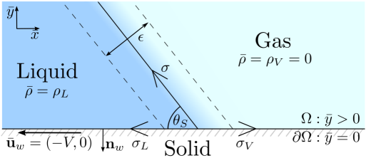
Figure 1: Sketch of the diffuse-interface model near a wall.

2 Problem specification

Consider the fluid domain $\Omega=\{\bar{x}\in\mathbb{R},0<\bar{y}\}$ (bars are used to denote dimensional variables) and the solid surface $\partial\Omega=\{\bar{x}\in\mathbb{R},\bar{y}=0\}$, where our frame of reference is with the moving contact line, such that the driving force is the wall velocity $\bar{\textbf{u}}_{w}$, see Fig. 1. We assume that the free energy of the system has contributions from an isothermal fluid with a Helmholtz free energy functional and from the wall energy, given by

$$\bar{\mathscr{F}}=\bar{\mathscr{F}}_{m}+\bar{\mathscr{F}}_{w}=\int_{\Omega}\bar{\mathcal{L}}\textrm{d}\Omega+\int_{\partial\Omega}\bar{f}_{w}(\bar{\rho})\textrm{d}A,\qquad\bar{\mathcal{L}}=\bar{\rho}\bar{f}(\bar{\rho})+\frac{1}{2}K|\bar{\bm{\nabla}}\bar{\rho}|^{2}-\bar{G}\bar{\rho},$$ (1)

where $\bar{G}$ is the chemical potential, a Lagrange multiplier introduced to ensure mass conservation, $K$ is a gradient energy coefficient (assumed to be a constant for simplicity, as suggested in Ref. ¹⁰), $\bar{f}_{w}(\bar{\rho})$ is the wall energy, to be defined when considering the boundary conditions, and $\bar{\rho}\bar{f}(\bar{\rho})$ is a double well potential chosen to give the two equilibrium states $\bar{\rho}=\{0,\rho_{L}\}$. In a similar way to a discussion in Ref. ³⁹, $\epsilon=(K\rho_{L}/\breve{F})^{1/2}$ is the characteristic thickness of the interface, where $\breve{F}$ is a characteristic value of $\bar{f}(\bar{\rho})$.

Forms such as in Eq. (1) for the free energy, and their corresponding diffuse-interface approximations, have been adopted by numerous authors for wetting problems such as Cahn,⁴¹ Seppecher,¹¹ Pismen and Pomeau,³⁹ and Pismen;⁴² see also the review by de Gennes.² This form of free energy is simplified in that it uses a local approximation to neglect non-local, integral, terms. The approximation effectively arises through a Taylor series expansion of the density, and retaining up to and including quadratic terms,^{42, 43} further details given in Appendix A. The effect of such non-local terms has been considered at equilibrium in studies such as in Refs. ⁴², ⁴³, where the long-range intermolecular interactions are responsible for an algebraic decay of the density profile away from the interface instead of the exponential one predicted by local models (seen for the model considered here, in Eq. (41)). In our dynamic situation, we focus on the local approximation to elucidate the contact line behaviour in a simplified, yet widely used and applicable setting.

The density field augments the usual hydrodynamic equations through an additional stress tensor, termed the capillary or Korteweg tensor, defined as

$$\bar{\textbf{T}}=\bar{\mathcal{L}}\textbf{I}-\bar{\bm{\nabla}}\bar{\rho}\otimes\frac{\partial{\bar{\mathcal{L}}}}{\partial{(\bar{\bm{\nabla}}\bar{\rho})}},$$ (2)

where I is the identity tensor, and which arises as a consequence of Noether’s theorem.^{44, 10} On using the assumed form of $\bar{\mathcal{L}}$ from (1) and coupling the capillary tensor with the usual viscous stress tensor $\bar{\bm{\tau}}$ in the compressible Navier-Stokes equations, with total stress tensor $\bar{\textbf{M}}$, the governing equations we thus consider are

$$\frac{\partial{\bar{\rho}}}{\partial{\bar{t}}}+\bar{\bm{\nabla}}\bm{\cdot}(\bar{\rho}\bar{\textbf{u}})=0,$$ (3)

$$\bar{\rho}\left(\frac{\partial{\bar{\textbf{u}}}}{\partial{\bar{t}}}+\bar{\textbf{u}}\bm{\cdot}\bar{\bm{\nabla}}\bar{\textbf{u}}\right)=\bar{\bm{\nabla}}\bm{\cdot}\bar{\textbf{M}},$$ (4)

with

$$\bar{\textbf{M}}=\bar{\textbf{T}}+\bar{\bm{\tau}},$$ (5)

$$\bar{\textbf{T}}=\left(\bar{\rho}\bar{f}(\bar{\rho})+\frac{K}{2}|\bar{\bm{\nabla}}\bar{\rho}|^{2}-\bar{G}\bar{\rho}\right)\textbf{I}-K\bar{\bm{\nabla}}\bar{\rho}\otimes\bar{\bm{\nabla}}\bar{\rho},$$ (6)

$$\bar{\bm{\tau}}=\bar{\mu}(\bar{\rho})\left[(\bar{\bm{\nabla}}\bar{\textbf{u}})+(\bar{\bm{\nabla}}\bar{\textbf{u}})^{\mathrm{T}}\right]+\bar{\nu}(\bar{\rho})\left[(\bar{\bm{\nabla}}\bm{\cdot}\bar{\textbf{u}})\textbf{I}\right],$$ (7)

$$\bar{G}=-K\bar{\nabla}^{2}\bar{\rho}+\frac{\partial{}}{\partial{\bar{\rho}}}(\bar{\rho}\bar{f}(\bar{\rho})),$$ (8)

where $\bar{\textbf{u}}$ is the fluid velocity, $\bar{\mu}(\bar{\rho})$ and $\bar{\nu}(\bar{\rho})$ are the fluid viscosities (depending on the density), and $\bar{t}$ is time. We have taken the viscous stress tensor $\bar{\bm{\tau}}$ to be Newtonian and the thermodynamic pressure is given by $\bar{p}=\bar{\rho}^{2}\bar{f}^{\prime}(\bar{\rho})$. The form for $\bar{G}$ arises from the Euler-Lagrange equation corresponding to the free energy, and will be motivated by considering the first variation of $\bar{\mathscr{F}}$ when discussing the wall boundary conditions at the end of this section (the mathematical motivation of the associated variational problem was discussed in the recent study in Ref. ⁴⁵).

For the analysis, we leave $\bar{\mu}(\bar{\rho})$, $\bar{\nu}(\bar{\rho})$ and $\bar{\rho}\bar{f}(\bar{\rho})$ general, but as mentioned in the introduction, for ease of comprehension and clarity, we will include results for the specific case considered in Ref. ⁴⁰, and displayed equations relating to this specific case will be labelled “SC”. This specific case used viscosity and density forms

$$\mbox{SC:}\qquad\bar{\mu}(\bar{\rho})=\frac{\mu_{L}}{\rho_{L}}\bar{\rho},\qquad\bar{\nu}(\bar{\rho})=-\frac{2}{3}\bar{\mu}(\bar{\rho})\qquad\bar{f}(\bar{\rho})=\frac{K}{2\epsilon^{2}}\bar{\rho}\left(1-\frac{\bar{\rho}}{\rho_{L}}\right)^{2},$$ (9)

where $\bar{\mu}(\bar{\rho})$ has the two equilibrium states at $\mu_{L}$ and $\mu_{V}=0$.

On the solid surface $\partial\Omega$, with normal $\textbf{n}_{w}$, we impose

$$\bar{\textbf{u}}=\bar{\textbf{u}}_{w},\qquad K\textbf{n}_{w}\bm{\cdot}\bar{\bm{\nabla}}\bar{\rho}+\bar{f}^{\prime}_{w}(\bar{\rho})=0,$$ (10)

with wall velocity $\bar{\textbf{u}}_{w}=(-V,0)$ in Cartesian coordinates at $\bar{y}=0$. The first condition is the classical no-slip, whilst the second arises through variational arguments, discussed at the end of this section, and is termed the natural (or wetting) boundary condition.⁴⁶ We note that this form of the natural boundary condition requires the wall free energy to instantaneously relax to equilibrium (as originally understood by Jacqmin ¹²). In the conclusion, another form will be discussed where a finite timescale for the relaxation is posited, allowing for dynamic microscopic contact angle variation. Although the analysis does not change significantly, we proceed with the above condition to demonstrate that this form is sufficient to resolve the singularities associated with the moving contact line problem—without this extra degree of freedom. The form for $\bar{f}_{w}$ should be chosen to satisfy Young’s law at the contact line, with solid-liquid, solid-gas and liquid-gas surface tensions $\bar{f}_{w}(\rho_{L})=\sigma_{L}$, $\bar{f}_{w}(0)=\sigma_{V}$ and $\sigma$, to be specified in (12), respectively, and with contact angle $\theta_{S}$. A cubic is the lowest-order polynomial required such that the wall free energy can be minimised for the bulk densities and prevent a precursor film (or enrichment/depletion) forming away from the contact line, i.e. $\bar{f}^{\prime}_{w}(\rho_{L})=\bar{f}^{\prime}_{w}(0)=0$. Whilst cubic forms are used for binary fluid problems, e.g. in Refs. ¹², ¹⁸, this is unlike the linear forms proposed in the previous studies for liquid-gas problems^{11, 13, 14, 47}, allowing us to consider a diffuse-interface model without further physical effects from the microscale. These requirements determine

$$\bar{f}_{w}(\bar{\rho})=\left[{{\rho_{L}^{-3}\sigma\cos\theta_{S}}(4\bar{\rho}^{3}-6\bar{\rho}^{2}\rho_{L}+\rho_{L}^{3})+\sigma_{V}+\sigma_{L}}\right]/2,$$ (11)

giving $\bar{f}^{\prime}_{w}(\bar{\rho})=-{6\sigma}\bar{\rho}\left(\rho_{L}-\bar{\rho}\right)\cos\theta_{S}/{\rho_{L}^{3}}$, and $\bar{f}_{w}(0)-\bar{f}_{w}(\rho_{L})=\sigma\cos\theta_{S}$, with Young’s law thus satisfied. It is noteworthy that the natural boundary condition may be replaced by a constant density condition if a precursor film/disjoining pressure model is to be considered, i.e. $\bar{\rho}=\rho_{a}$ on $\partial\Omega$ (as used by Pismen and Pomeau³⁹), although as we shall demonstrate, this model is not necessary to remove the singularities associated with the moving contact line. Finally, for a one-dimensional density profile $\bar{\rho}(\bar{z})$ in equilibrium the surface tension across the interface is⁴⁸

$$\sigma=K\int_{-\infty}^{\infty}\left(\frac{\textrm{d}\bar{\rho}}{\textrm{d}\bar{z}}\right)^{2}\,\textrm{d}\bar{z}=\sqrt{2K}\int_{0}^{\rho_{L}}\sqrt{\bar{\rho}[\bar{f}(\bar{\rho})-\bar{G}_{e}]}\,\textrm{d}\bar{\rho},$$ (12)

which for the specific double well form in (9), considered in Ref. ⁴⁰, this gives

$$\mbox{SC:}\qquad\sigma=\frac{K\rho_{L}^{2}}{6\epsilon}.$$ (13)

We note that equilibrium occurs in the governing equations when $\bar{\textbf{u}}=0$ and when $\bar{G}=\bar{G}_{e}$, a constant which is chosen such that $\bar{\rho}\bar{f}(\bar{\rho})$ predicts equally stable bulk fluids. In (12), $\bar{G}_{e}$ is unknown, but it may be assumed that $\bar{\rho}\bar{f}(\bar{\rho})$ is chosen in such a way to require $\bar{G}_{e}=0$ (i.e. $[\bar{\rho}\bar{f}(\bar{\rho})]|_{\bar{\rho}=\rho_{L}}=[\bar{\rho}\bar{f}(\bar{\rho})]|_{\bar{\rho}=0}$), and in particular this is true of the form in (9).

We now briefly describe how the natural boundary condition and the chemical potential arise. Consider the first variation of the total free energy $\bar{\mathscr{F}}$, i.e. consider

$$\left.{\frac{\delta}{\delta\varepsilon}\left({\bar{\mathscr{F}}[\bar{\rho}+\varepsilon{\bar{\rho}^{*}}]}\right)}\right|_{\varepsilon=0}=0,$$ (14)

where $\bar{\rho}^{*}$ is the increment of the density, so that

$$0= \int_{\Omega}\left\{{K(\bar{\bm{\nabla}}\bar{\rho})\bm{\cdot}(\bar{\bm{\nabla}}{\bar{\rho}^{*}})+\left[{{\bar{\rho}^{*}}\bar{f}(\bar{\rho})+\bar{\rho}{\bar{\rho}^{*}}\bar{f}^{\prime}(\bar{\rho})}\right]-\bar{G}{\bar{\rho}^{*}}}\right\}\textrm{d}\Omega+\int_{\partial\Omega}{\bar{\rho}^{*}}\bar{f}_{w}^{\prime}(\bar{\rho})\textrm{d}A,$$ (15)

thus

$$0= \int_{\Omega}\left\{{K\left[{\bar{\bm{\nabla}}\bm{\cdot}({\bar{\rho}^{*}}\bar{\bm{\nabla}}\bar{\rho})-{\bar{\rho}^{*}}\bar{\bm{\nabla}}\bm{\cdot}(\bar{\bm{\nabla}}\bar{\rho})}\right]+{\bar{\rho}^{*}}\bar{f}(\bar{\rho})+\bar{\rho}{\bar{\rho}^{*}}\bar{f}^{\prime}(\bar{\rho})-\bar{G}{\bar{\rho}^{*}}}\right\}\textrm{d}\Omega+\int_{\partial\Omega}{\bar{\rho}^{*}}\bar{f}_{w}^{\prime}(\bar{\rho})\textrm{d}A.$$ (16)

Applying the divergence theorem, this becomes

$$0= \int_{\Omega}-K{\bar{\rho}^{*}}\bar{\bm{\nabla}}\bm{\cdot}(\bar{\bm{\nabla}}\bar{\rho})+{\bar{\rho}^{*}}\bar{f}(\bar{\rho})+\bar{\rho}{\bar{\rho}^{*}}\bar{f}^{\prime}(\bar{\rho})-\bar{G}{\bar{\rho}^{*}}\textrm{d}\Omega+\int_{\partial\Omega}K\textbf{n}_{w}\bm{\cdot}({\bar{\rho}^{*}}\bar{\bm{\nabla}}\bar{\rho})+{\bar{\rho}^{*}}\bar{f}_{w}^{\prime}(\bar{\rho})\textrm{d}A,$$

$$= \int_{\Omega}{\bar{\rho}^{*}}\left[{\bar{f}(\bar{\rho})+\bar{\rho}\bar{f}^{\prime}(\bar{\rho})-\bar{G}-K\bar{\bm{\nabla}}\bm{\cdot}(\bar{\bm{\nabla}}\bar{\rho})}\right]\textrm{d}\Omega+\int_{\partial\Omega}{\bar{\rho}^{*}}\left[{K\textbf{n}_{w}\bm{\cdot}\bar{\bm{\nabla}}\bar{\rho}+\bar{f}_{w}^{\prime}(\bar{\rho})}\right]\textrm{d}A,$$

$$= \int_{\Omega}{\bar{\rho}^{*}}\left[{\frac{\partial{}}{\partial{\bar{\rho}}}[\bar{\rho}\bar{f}(\bar{\rho})]-\bar{G}-K\bar{\nabla}^{2}\bar{\rho}}\right]\textrm{d}\Omega+\int_{\partial\Omega}{\bar{\rho}^{*}}\left[{K\textbf{n}_{w}\bm{\cdot}\bar{\bm{\nabla}}\bar{\rho}+\bar{f}_{w}^{\prime}(\bar{\rho})}\right]\textrm{d}A,$$ (17)

and as this is true for any increment ${\bar{\rho}^{*}}$, then the bulk chemical potential is specified by

$$\bar{G}=\frac{\partial{}}{\partial{\bar{\rho}}}[\bar{\rho}\bar{f}(\bar{\rho})]-K\bar{\nabla}^{2}\bar{\rho},\qquad\mbox{in }\Omega,$$ (18)

and $\bar{\rho}$ must satisfy the natural boundary condition

$$K\textbf{n}_{w}\bm{\cdot}\bar{\bm{\nabla}}\bar{\rho}+\bar{f}_{w}^{\prime}(\bar{\rho})=0,\qquad\mbox{on }\partial\Omega.$$ (19)

The normal $\textbf{n}_{w}$ has arisen through application of the divergence theorem above, and thus must be defined as the outward unit normal to $\Omega$ on the boundary $\partial\Omega$. In Cartesian components and for our geometry $\textbf{n}_{w}=(0,-1)$, and the natural boundary condition thus gives

$$-K\frac{\partial{\bar{\rho}}}{\partial{\bar{y}}}+\bar{f}_{w}^{\prime}(\bar{\rho})=0,\qquad\mbox{on }\bar{y}=0.$$ (20)

3 Nondimensionalization of the model and other representations

We introduce the scalings

$$\bar{x}=Xx,\quad\bar{y}=Xy,\quad\bar{\textbf{u}}=V\textbf{u},\quad\bar{t}=\frac{X}{V}t,\quad\bar{\rho}=\rho_{L}\rho,\quad\bar{p}=\frac{\mu_{L}V}{X}p,$$

$$\bar{G}=\frac{K\rho_{L}}{\epsilon X}G,\quad\bar{f}=\breve{F}f=\frac{K\rho_{L}}{\epsilon^{2}}f,\quad\bar{\textbf{M}}=\frac{\mu_{L}V}{X}\textbf{M},\quad\bar{\textbf{T}}=\frac{K\rho_{L}^{2}}{\epsilon X}\textbf{T},\quad\bar{\bm{\tau}}=\frac{\mu_{L}V}{X}\bm{\tau},$$ (21)

where $X$ is a typical length scale (which would be based on the macroscopic geometry, such as a channel width or droplet radius, for instance), $V$ is a typical velocity scale (we choose this based on the wall velocity in the $x$-direction), and we nondimensionalize $\bar{\rho}$ with the bulk liquid density. The other scalings arise from balances in the governing equations, and will contain the nondimensional parameters

$$\operatorname{Ca}=\frac{\mu_{L}V}{\sigma},\quad\operatorname{Cn}=\frac{\epsilon}{X},\quad\operatorname{Re}=\frac{\rho_{L}VX}{\mu_{L}},\quad\operatorname{Ca}_{K}=\frac{\mu_{L}V\epsilon}{K\rho_{L}^{2}},$$ (22)

being the usual Capillary number, Cahn number and Reynolds number, and a modified Capillary number based on the model parameter $K$, respectively. We describe $\operatorname{Ca}_{K}$ as a modified Capillary number as for a given free-energy form , the modified number and the usual one, are directly proportional through the non-dimensional version of Eq. (12) (given later in Eq. (33)). The governing equations become

$$\frac{\partial{\rho}}{\partial{t}}+\bm{\nabla}\bm{\cdot}(\rho\textbf{u}) =0,$$ (23)

$$\operatorname{Re}\rho\left(\frac{\partial{\textbf{u}}}{\partial{t}}+\textbf{u}\bm{\cdot}\bm{\nabla}\textbf{u}\right) =\bm{\nabla}\bm{\cdot}\textbf{M},$$ (24)

M $$=\frac{1}{\operatorname{Ca}_{K}}\textbf{T}+\bm{\tau},$$ (25)

T $$=\left(\frac{1}{\operatorname{Cn}}\rho f(\rho)+\frac{\operatorname{Cn}}{2}|\bm{\nabla}\rho|^{2}-G\rho\right)\textbf{I}-\operatorname{Cn}\bm{\nabla}\rho\otimes\bm{\nabla}\rho,$$ (26)

$$\bm{\tau} =\mu(\rho)\left[{(\bm{\nabla}\textbf{u})+(\bm{\nabla}\textbf{u})^{\mathrm{T}}}\right]+\nu(\rho)(\bm{\nabla}\bm{\cdot}\textbf{u})\textbf{I},$$ (27)

$$G =-\operatorname{Cn}\nabla^{2}\rho+\frac{1}{\operatorname{Cn}}\frac{\partial{}}{\partial{\rho}}(\rho f(\rho)),$$ (28)

$$p =(\operatorname{Cn}\operatorname{Ca}_{K})^{-1}\rho^{2}f^{\prime}(\rho),$$ (29)

and we note the nondimensional general viscosity functions $\mu(\rho)$ and $\nu(\rho)$. As discussed, in contrast to the analysis in Ref. ⁴⁰ we leave the free energy component $f(\rho)$ general, and thus also the pressure, but note the specific case considered there had

$$\mbox{SC:}\qquad f(\rho)=\frac{1}{2}\rho(1-\rho)^{2},\qquad\mbox{and thus}\qquad p=\frac{1}{2\operatorname{Cn}\operatorname{Ca}_{K}}\rho^{2}(1-3\rho)(1-\rho).$$ (30)

On the solid surface $\partial\Omega$, we have

$$\textbf{u}=\textbf{u}_{w},\qquad\operatorname{Cn}\frac{\operatorname{Ca}}{\operatorname{Ca}_{K}}\textbf{n}_{w}\bm{\cdot}\bm{\nabla}\rho=6\cos\theta_{S}(1-\rho)\rho,$$ (31)

where $\textbf{u}_{w}$ is the (now non-dimensional) wall velocity, satisfying $\textbf{u}_{w}=(-1,0)$ in Cartesian components, and in equilibrium for the one dimensional variation of $\rho(z)$ across the interface (being the equivalent nondimensional expression of (12))

$$\frac{\operatorname{Ca}_{K}}{\operatorname{Cn}\operatorname{Ca}} =\int_{-\infty}^{\infty}\left(\frac{\textrm{d}\rho}{\textrm{d}z}\right)^{2}\ \textrm{d}z=\int_{-\infty}^{\infty}\sqrt{\frac{2}{\operatorname{Cn}^{2}}\rho f}\frac{\textrm{d}\rho}{\textrm{d}z}\ \textrm{d}z=\frac{\sqrt{2}}{\operatorname{Cn}}\int_{0}^{1}\sqrt{\rho f}\ {\textrm{d}\rho},$$ (32)

suggesting

$${\operatorname{Ca}_{K}}={\sqrt{2}}\operatorname{Ca}\int_{0}^{1}\sqrt{\rho f}\ {\textrm{d}\rho},$$ (33)

which for the specific case gives

$$\mbox{SC:}\qquad{\operatorname{Ca}}={6}{\operatorname{Ca}_{K}},\qquad\operatorname{Cn}\textbf{n}_{w}\bm{\cdot}\bm{\nabla}\rho=\cos\theta_{S}(1-\rho)\rho,$$ (34)

so that in this particular instance there is no Capillary number, $\operatorname{Ca}$, as part of the governing equations or boundary conditions—the problem then depends only upon $\operatorname{Cn}$, $\operatorname{Ca}_{K}$ and $\operatorname{Re}$. As mentioned, we will leave this general, however, and not choose a specific $f(\rho)$.

3.1 The combined form of the model

We can combine many of the equations into a single equation, noting that a similar combined equation form has been used in Ref. ³⁹ when considering a diffuse-interface model with a precursor film in the lubrication approximation. From (27) we determine

$$\bm{\nabla}\bm{\cdot}\bm{\tau} =\mu(\rho)\bm{\nabla}^{2}\textbf{u}+[\mu(\rho)+\nu(\rho)]\bm{\nabla}(\bm{\nabla}\bm{\cdot}\textbf{u})+\left[{(\bm{\nabla}\textbf{u})+(\bm{\nabla}\textbf{u})^{\mathrm{T}}}\right]\bm{\nabla}(\mu(\rho))+\bm{\nabla}(\nu(\rho))(\bm{\nabla}\bm{\cdot}\textbf{u})\textbf{I},$$ (35)

and by using (26) and (28)

$$\bm{\nabla}\bm{\cdot}\textbf{T} =\bm{\nabla}\bm{\cdot}\left[\left(\frac{1}{\operatorname{Cn}}\rho f(\rho)+\frac{\operatorname{Cn}}{2}|\bm{\nabla}\rho|^{2}+\operatorname{Cn}\rho\nabla^{2}\rho-\frac{\rho}{\operatorname{Cn}}\frac{\partial{}}{\partial{\rho}}(\rho f(\rho))\right)\textbf{I}-\operatorname{Cn}\bm{\nabla}\rho\otimes\bm{\nabla}\rho\right]$$

$$=\bm{\nabla}\left(\frac{\operatorname{Cn}}{2}|\bm{\nabla}\rho|^{2}+\operatorname{Cn}\rho\nabla^{2}\rho-\operatorname{Ca}_{K}p\right)-\operatorname{Cn}\bm{\nabla}\bm{\cdot}(\bm{\nabla}\rho\otimes\bm{\nabla}\rho)$$

$$=\operatorname{Cn}\rho\bm{\nabla}(\nabla^{2}\rho)-\operatorname{Ca}_{K}\bm{\nabla}p,$$ (36)

so that for the creeping flow case, where inertial forces are negligible if compared to viscous forces, i.e. $\operatorname{Re}\ll 1$, we have

$$\bm{\nabla}\bm{\cdot}\textbf{M} =\frac{1}{\operatorname{Ca}_{K}}\bm{\nabla}\bm{\cdot}\textbf{T}+\bm{\nabla}\bm{\cdot}\bm{\tau}$$

$$=\frac{\operatorname{Cn}}{\operatorname{Ca}_{K}}\rho\bm{\nabla}(\nabla^{2}\rho)-\bm{\nabla}p+\mu(\rho)\bm{\nabla}^{2}\textbf{u}+[\mu(\rho)+\nu(\rho)]\bm{\nabla}(\bm{\nabla}\bm{\cdot}\textbf{u})$$

$$\qquad\qquad\qquad\qquad\qquad+\left[{(\bm{\nabla}\textbf{u})+(\bm{\nabla}\textbf{u})^{\mathrm{T}}}\right]\bm{\nabla}(\mu(\rho))+\bm{\nabla}(\nu(\rho))(\bm{\nabla}\bm{\cdot}\textbf{u})\textbf{I}$$

$$=0,$$ (37)

with $p=(\operatorname{Cn}\operatorname{Ca}_{K})^{-1}\rho^{2}f^{\prime}(\rho)$, the continuity equation (23) coupled, and the boundary conditions on $\partial\Omega$ remaining as in Eq. (31).

3.2 Equilibrium solution

To draw comparisons to previous work, and to give a basis for comparison when the dynamic contact line behaviour is analysed, we consider the equilibrium behaviour of the system, corresponding to $\operatorname{Ca}_{K}\ll 1$. It is clear from Eqs. (23)–(29) that this corresponds to the capillary tensor dominating, and thus $\bm{\nabla}\bm{\cdot}\textbf{T}=0$. The equilibrium solution is thus governed by

$${\operatorname{Cn}^{2}}\rho\bm{\nabla}(\nabla^{2}\rho)=\bm{\nabla}\left[{\rho^{2}f^{\prime}(\rho)}\right],$$ (38)

subject to the natural boundary condition $-[\operatorname{Cn}\operatorname{Ca}/(6\operatorname{Ca}_{K})]\partial_{y}{\rho}=\cos\theta_{S}(1-\rho)\rho$ at $y=0$, and the expected bulk behaviour $\rho\to\{0,1\}$ and $\nabla^{2}\rho\to 0$ as $x\to\pm\infty$. Considering the equation, we do not want the trivial solution, and so expansion of the gradient and simplifying leads to

$${\operatorname{Cn}^{2}}\bm{\nabla}(\nabla^{2}\rho)=\left({2f^{\prime}(\rho)+\rho f^{\prime\prime}(\rho)}\right)\bm{\nabla}\rho.$$ (39)

This vector equation may be integrated once to obtain the scalar equation

$${\operatorname{Cn}^{2}}(\nabla^{2}\rho)=\rho f^{\prime}(\rho)+f(\rho)=\frac{\partial{}}{\partial{\rho}}(\rho f(\rho)),$$ (40)

having removed arbitrary constants as we expect $\nabla^{2}\rho\to 0$ and $\partial_{\rho}{}(\rho f(\rho))\to 0$ (i.e. the double well potential is minimised) far away from the interface.

The solution subject to the above conditions for the specific function $f(\rho)$ in (30), considered in Ref. ⁴⁰ is

$$\mbox{SC:}\qquad\rho=\frac{1}{2}\left({1-\tanh\left[{\frac{x\sin\theta_{S}+y\cos\theta_{S}}{2\operatorname{Cn}}}\right]}\right),$$ (41)

having also fixed the interface at $\rho=1/2$. This profile is planar and at angle $\theta_{S}$. Similar hyperbolic tangent or exponential behaviours for equilibrium solutions have been seen in many diffuse-interface and phase-field models, such as in Refs. ³⁹, ⁴⁶, ¹⁸, ⁴⁹, ⁵⁰, ¹², ⁴⁸, ¹⁴, ¹⁶, ⁵¹, it being a signature of diffuse-interface models with a local approximation.

As discussed in the introduction, the density variation for physical systems between liquid and gas occurs on a length scale which is much smaller than the macroscopic length scale, and hence $\operatorname{Cn}={\epsilon}/{X}\ll 1$. The sharp-interface limit is given by the asymptotic behaviour as $\operatorname{Cn}\to 0$, and understanding the behaviour of the governing equations in this limit is of central importance when considering diffuse-interface models, as the classical continuum models (as given in e.g. Ref. ⁵²) should be recovered if correct predictions are to be found.

We will next undertake a careful asymptotic analysis of the outer solution away from the interface, and of the interfacial region away from the wall (using body fitted coordinates), to show that the expected sharp-interface equations (the Navier–Stokes equations and the usual capillary surface stress conditions) are indeed recovered.

4 Sharp-interface limit away from the walls

4.1 The outer (bulk) regions

We consider the governing equations (23)–(29). In the outer region for the bulk fluids away from the interface, where variables are denoted with ^±, we consider $\operatorname{Cn}\to 0$ and take the expansions

$$\rho(t,x,y) =\rho_{0}^{\pm}+\operatorname{Cn}\rho_{1}^{\pm}+\operatorname{Cn}^{2}\rho_{2}^{\pm}+\cdots, G(t,x,y) ={G}_{0}^{\pm}+\operatorname{Cn}{G}_{1}^{\pm}+\operatorname{Cn}^{2}{G}_{2}^{\pm}+\cdots,$$

$$\textbf{u}(t,x,y) ={\textbf{u}}_{0}^{\pm}+\operatorname{Cn}{\textbf{u}}_{1}^{\pm}+\operatorname{Cn}^{2}{\textbf{u}}_{2}^{\pm}+\cdots, p(t,x,y) ={p}_{0}^{\pm}+\operatorname{Cn}{p}_{1}^{\pm}+\operatorname{Cn}^{2}{p}_{2}^{\pm}+\cdots,$$

$$\textbf{M}(t,x,y) =\textbf{M}_{0}^{\pm}+\operatorname{Cn}\textbf{M}_{1}^{\pm}+\operatorname{Cn}^{2}\textbf{M}_{2}^{\pm}+\cdots, \textbf{T}(t,x,y) =\textbf{T}_{0}^{\pm}+\operatorname{Cn}\textbf{T}_{1}^{\pm}+\operatorname{Cn}^{2}\textbf{T}_{2}^{\pm}+\cdots,$$

$$\bm{\tau}(t,x,y) =\bm{\tau}_{0}^{\pm}+\operatorname{Cn}\bm{\tau}_{1}^{\pm}+\operatorname{Cn}^{2}\bm{\tau}_{2}^{\pm}+\cdots,$$ (42)

where for example $\rho_{0}^{+}$ is in the region of the liquid, see Fig. 1. At leading order, $O(\operatorname{Cn}^{-1})$, we find that

$$\rho_{0}^{\pm}f(\rho_{0}^{\pm})=\frac{\partial{}}{\partial{\rho}}(\rho_{0}^{\pm}f(\rho_{0}^{\pm}))=0,$$ (43)

from the chemical potential equation, determining that the two free energy minima corresponding to the liquid and gas bulk values are the two solutions for $\rho_{0}^{\pm}$. This then implies

$$\rho_{0}^{\pm}f^{\prime}(\rho_{0}^{\pm})+f(\rho_{0}^{\pm})=0\quad\Rightarrow\quad\rho_{0}^{\pm 2}f^{\prime}(\rho_{0}^{\pm})+\rho_{0}^{\pm}f(\rho_{0}^{\pm})=0\quad\Rightarrow\quad\rho_{0}^{\pm 2}f^{\prime}(\rho_{0}^{\pm})=0,$$ (44)

being consistent with zero pressure at this order. The $O(1)$ equations then give

$$\rho_{0}^{\pm}\bm{\nabla}\bm{\cdot}\textbf{u}_{0}^{\pm} =0,$$ (45)

$$\operatorname{Re}\rho_{0}^{\pm}\left(\frac{\partial{\textbf{u}_{0}^{\pm}}}{\partial{t}}+\textbf{u}_{0}^{\pm}\bm{\cdot}\bm{\nabla}\textbf{u}_{0}^{\pm}\right) =\bm{\nabla}\bm{\cdot}\textbf{M}_{0}^{\pm},$$ (46)

$$\textbf{M}_{0}^{\pm} =\frac{1}{\operatorname{Ca}_{K}}\textbf{T}_{0}^{\pm}+\bm{\tau}_{0}^{\pm},$$ (47)

$$\textbf{T}_{0}^{\pm} =\left(\rho_{1}^{\pm}(\rho_{0}^{\pm}f^{\prime}(\rho_{0}^{\pm})+f(\rho_{0}^{\pm}))-G_{0}^{\pm}\rho_{0}^{\pm}\right)\textbf{I}=-G_{0}^{\pm}\rho_{0}^{\pm}\textbf{I},$$ (48)

$$\bm{\tau}_{0}^{\pm} =\mu(\rho_{0}^{\pm})\left[{(\bm{\nabla}\textbf{u}_{0}^{\pm})+(\bm{\nabla}\textbf{u}_{0}^{\pm})^{\mathrm{T}}}\right]+\nu(\rho_{0}^{\pm})(\bm{\nabla}\bm{\cdot}\textbf{u}_{0}^{\pm})\textbf{I},$$ (49)

$$G_{0}^{\pm} =\rho_{1}^{\pm}(\rho_{0}^{\pm}f^{\prime\prime}(\rho_{0}^{\pm})+2f^{\prime}(\rho_{0}^{\pm})),$$ (50)

$$p_{0}^{\pm} =\frac{1}{\operatorname{Ca}_{K}}\rho_{0}^{\pm}\rho_{1}^{\pm}(\rho_{0}^{\pm}f^{\prime\prime}(\rho_{0}^{\pm})+2f^{\prime}(\rho_{0}^{\pm})),$$ (51)

which simplify to

$$\rho_{0}^{\pm}\bm{\nabla}\bm{\cdot}\textbf{u}_{0}^{\pm}=0,\qquad\operatorname{Re}\rho_{0}^{\pm}\left(\frac{\partial{\textbf{u}_{0}^{\pm}}}{\partial{t}}+\textbf{u}_{0}^{\pm}\bm{\cdot}\bm{\nabla}\textbf{u}_{0}^{\pm}\right)=\bm{\nabla}\bm{\cdot}\textbf{M}_{0}^{\pm},\qquad\textbf{M}_{0}^{\pm}=-p_{0}^{\pm}\textbf{I}+\bm{\tau}_{0}^{\pm},$$ (52)

since

$$\textbf{T}_{0}^{\pm}=-G_{0}^{\pm}\rho_{0}^{\pm}\textbf{I},\qquad\mbox{and}\qquad G_{0}^{\pm}={\operatorname{Ca}_{K}}\left({\frac{p_{0}^{\pm}}{\rho_{0}^{\pm}}}\right).$$ (53)

This is an important result, as we see that at leading order the governing equations are the expected incompressible Navier–Stokes equations. The equations at the next order, $O(\operatorname{Cn})$, are

$$\frac{\partial{\rho_{1}^{\pm}}}{\partial{t}}+\bm{\nabla}\bm{\cdot}(\rho_{1}^{\pm}\textbf{u}_{0}^{\pm})+\rho_{0}^{\pm}\bm{\nabla}\bm{\cdot}\textbf{u}_{1}^{\pm} =0,$$ (54)

$$\operatorname{Re}\left[\rho_{1}^{\pm}\left(\frac{\partial{\textbf{u}_{0}^{\pm}}}{\partial{t}}+\textbf{u}_{0}^{\pm}\bm{\cdot}\bm{\nabla}\textbf{u}_{0}^{\pm}\right)+\rho_{0}^{\pm}\left(\frac{\partial{\textbf{u}_{1}^{\pm}}}{\partial{t}}+\textbf{u}_{1}^{\pm}\bm{\cdot}\bm{\nabla}\textbf{u}_{0}^{\pm}+\textbf{u}_{0}^{\pm}\bm{\cdot}\bm{\nabla}\textbf{u}_{1}^{\pm}\right)\right] =\bm{\nabla}\bm{\cdot}\textbf{M}_{1}^{\pm},$$ (55)

where

$$\textbf{M}_{1}^{\pm} =\frac{1}{\operatorname{Ca}_{K}}\textbf{T}_{1}^{\pm}+\bm{\tau}_{1}^{\pm},$$ (56)

$$\textbf{T}_{1}^{\pm} =\left(\rho_{2}^{\pm}\left[{\rho_{0}^{\pm}f^{\prime}(\rho_{0}^{\pm})+f(\rho_{0}^{\pm})}\right]+\rho_{1}^{\pm 2}\left[{f^{\prime}(\rho_{0}^{\pm})+\frac{1}{2}\rho_{0}^{\pm}f^{\prime\prime}(\rho_{0}^{\pm})}\right]-G_{1}^{\pm}\rho_{0}^{\pm}-G_{0}^{\pm}\rho_{1}^{\pm}\right)\textbf{I},$$ (57)

$$\bm{\tau}_{1}^{\pm} =\mu(\rho_{0}^{\pm})\left[{(\bm{\nabla}\textbf{u}_{1}^{\pm})+(\bm{\nabla}\textbf{u}_{1}^{\pm})^{\mathrm{T}}}\right]+\nu(\rho_{0}^{\pm})(\bm{\nabla}\bm{\cdot}\textbf{u}_{1}^{\pm})\textbf{I}+\rho_{1}^{\pm}\mu^{\prime}(\rho_{0}^{\pm})\left[{(\bm{\nabla}\textbf{u}_{0}^{\pm})+(\bm{\nabla}\textbf{u}_{0}^{\pm})^{\mathrm{T}}}\right]+\rho_{1}^{\pm}\nu^{\prime}(\rho_{0}^{\pm})(\bm{\nabla}\bm{\cdot}\textbf{u}_{0}^{\pm})\textbf{I},$$ (58)

$$G_{1}^{\pm} =\frac{1}{2}\rho_{1}^{\pm 2}\left[{3f^{\prime\prime}(\rho_{0}^{\pm})+\rho_{0}^{\pm}f^{\prime\prime\prime}(\rho_{0}^{\pm})}\right]+\rho_{2}^{\pm}\left[{2f^{\prime}(\rho_{0}^{\pm})+\rho_{0}^{\pm}f^{\prime\prime}(\rho_{0}^{\pm})}\right],$$ (59)

$$p_{1}^{\pm} =\frac{1}{\operatorname{Ca}_{K}}\left\{{\rho_{0}^{\pm}\rho_{2}^{\pm}\left[{2f^{\prime}(\rho_{0}^{\pm})+\rho_{0}^{\pm}f^{\prime\prime}(\rho_{0}^{\pm})}\right]+\rho_{1}^{\pm 2}\left[{\frac{1}{2}\rho_{0}^{\pm 2}f^{\prime\prime\prime}(\rho_{0}^{\pm})+f^{\prime}(\rho_{0}^{\pm})+2\rho_{0}^{\pm}f^{\prime\prime}(\rho_{0}^{\pm})}\right]}\right\},$$ (60)

being linear in $\rho_{2}^{\pm}$. The chemical potential and pressure terms may be used to determine

$$\textbf{T}_{1}^{\pm}=-\operatorname{Ca}_{K}p_{1}^{\pm}\textbf{I},$$ (61)

and thus a linearised form of the (compressible) Navier-Stokes equations is recovered.

4.2 The interface region

To consider the region near to the interface, the equations are transformed into body fitted coordinates $(\xi,\eta)$. $\xi$ measures distance along the interface (like an arc length), and $\eta$ measures the distance in the normal direction from a general point $(x,y)\in\Omega$ to the interface. For details see Appendix B.

We take the stretched coordinate $\zeta=\eta/\operatorname{Cn}$ to examine the region close to the interface. With this, we now have the interface satisfying $\zeta=\eta=0$, and we note that $\eta>0$ in the liquid (and $\eta<0$ in the gas) with n then pointing from gas to liquid. We take the limit $\operatorname{Cn}\to 0$ through the expansions

$$\rho =\breve{\rho}_{0}+\operatorname{Cn}\breve{\rho}_{1}+\operatorname{Cn}^{2}\breve{\rho}_{2}+\cdots, G =\breve{G}_{0}+\operatorname{Cn}\breve{G}_{1}+\operatorname{Cn}^{2}\breve{G}_{2}+\cdots,$$

u $$=\breve{\textbf{u}}_{0}+\operatorname{Cn}\breve{\textbf{u}}_{1}+\operatorname{Cn}^{2}\breve{\textbf{u}}_{2}+\cdots, \bm{\tau} =\frac{1}{\operatorname{Cn}}\left[\breve{\bm{\tau}}_{0}+\operatorname{Cn}\breve{\bm{\tau}}_{1}+\operatorname{Cn}^{2}\breve{\bm{\tau}}_{2}+\cdots\right],$$

T $$=\frac{1}{\operatorname{Cn}}\left[\breve{\textbf{T}}_{0}+\operatorname{Cn}\breve{\textbf{T}}_{1}+\operatorname{Cn}^{2}\breve{\textbf{T}}_{2}+\cdots\right], =\frac{1}{\operatorname{Cn}}\left[\breve{\textbf{M}}_{0}+\operatorname{Cn}\breve{\textbf{M}}_{1}+\operatorname{Cn}^{2}\breve{\textbf{M}}_{2}+\cdots\right],$$ M

$$p =\frac{1}{\operatorname{Cn}}\left[\breve{p}_{0}+\operatorname{Cn}\breve{p}_{1}+\operatorname{Cn}^{2}\breve{p}_{2}+\cdots\right].$$ (62)

Matching between interfacial variables, denoted $\breve{\phi}$ for an arbitrary function $\phi$, and outer variables (denoted $\phi^{\pm}$) is next considered. For this arbitrary function, we require $\phi^{\pm}(\xi,\eta)=\phi^{\pm}(\xi,\operatorname{Cn}\zeta)\sim\breve{\phi}(\xi,\zeta)$ for $\zeta\to\infty$, $\operatorname{Cn}\to 0$, $\operatorname{Cn}\zeta\to 0$. Thus

$$\phi^{\pm}(\xi,\operatorname{Cn}\zeta) =\phi^{\pm}_{0}(\xi,0)+\operatorname{Cn}\left(\zeta\frac{\partial{\phi^{\pm}_{0}}}{\partial{\zeta}}(\xi,0)+\phi^{\pm}_{1}(\xi,0)\right)+\cdots,$$

$$\breve{\phi}(\xi,\zeta) =\breve{\phi}_{0}(\xi,\zeta)+\operatorname{Cn}\breve{\phi}_{1}(\xi,\zeta)+\cdots,$$ (63)

which gives the first two matching conditions at $O(1)$ and $O(\operatorname{Cn})$ as

$$\lim_{\zeta\to\pm\infty}\breve{\phi}_{0}(\xi,\zeta) =\phi_{0}^{\pm}(\xi,0),$$ (64)

$$\lim_{\zeta\to\pm\infty}\breve{\phi}_{1}(\xi,\zeta) =\phi_{1}^{\pm}(\xi,0)+\zeta\frac{\partial{\phi_{0}^{\pm}}}{\partial{\zeta}}(\xi,0),$$ (65)

together implying

$$\lim_{\zeta\to\pm\infty}\frac{\partial{\breve{\phi_{1}}}}{\partial{\zeta}}(\xi,\zeta)=\frac{\partial{\phi_{0}^{\pm}}}{\partial{\zeta}}(\xi,0).$$ (66)

Using the details from Appendix B, we now go through each of the equations in turn and match to the outer region to determine the effective interfacial conditions in the sharp-interface limit.

4.2.1 Continuity equation

The continuity equation in body fitted coordinates and in the interfacial region is

$$\frac{\partial{{\rho}}}{\partial{t}}+\frac{u^{s}_{t}}{(1-\kappa\operatorname{Cn}\zeta)^{2}}\frac{\partial{{\rho}}}{\partial{\xi}}+\frac{u^{s}_{n}}{\operatorname{Cn}}\frac{\partial{{\rho}}}{\partial{\zeta}}+\frac{1}{\operatorname{Cn}}\frac{\partial{({\rho}v)}}{\partial{\zeta}}-\frac{\kappa{\rho}v}{1-\kappa\operatorname{Cn}\zeta}+\frac{\partial{({\rho}{u})}}{\partial{\xi}}=\operatorname{Cn}\frac{{\rho}{u}\zeta}{1-\kappa\operatorname{Cn}\zeta}\frac{\partial{\kappa}}{\partial{\xi}},$$ (67)

where $u^{s}_{t}$, $u^{s}_{n}$ are the tangential and normal velocities of the interface respectively, and assumed to be $O(1)$. $\kappa$ is the interfacial curvature, and $(u,v)$ are the velocity components in the $(\xi,\zeta)$ directions.

Considering expansions (62), then the leading order of the continuity equation satisfies

$${u^{s}_{n}}\frac{\partial{\breve{\rho_{0}}}}{\partial{\zeta}}+\frac{\partial{(\breve{\rho}_{0}\breve{v}_{0})}}{\partial{\zeta}}=0.$$ (68)

Assuming that the normal velocity of the interface is independent of the coordinate normal to the interface $\zeta$, then the leading order equation suggests

$$\left[\breve{\rho_{0}}({u^{s}_{n}}+\breve{v}_{0})\right]_{-\infty}^{\infty}=0,\quad\mbox{which implies}\quad{v}^{+}_{0}(0)=-{u^{s}_{n}},$$ (69)

and being equivalent to

$$\frac{\partial{d}}{\partial{t}}+\textbf{u}_{0}^{\pm}\bm{\cdot}\bm{\nabla}d=0,$$ (70)

the expected kinematic boundary condition for the sharp interface⁵² defined by $d(\textbf{x},t)=0$, where $d$ is the signed distance to the interface, equivalent to $\eta$.

4.2.2 Chemical potential equation

We now consider the chemical potential equation in the interfacial region

$$\operatorname{Cn}G=\frac{\partial{}}{\partial{\rho}}(\rho f(\rho))-\operatorname{Cn}^{2}\left[\frac{\partial^{2}_{\xi}{\rho}}{(1-\kappa\operatorname{Cn}\zeta)^{2}}+\frac{\operatorname{Cn}\zeta(\partial_{\xi}{\kappa})}{(1-\kappa\operatorname{Cn}\zeta)^{3}}\frac{\partial{\rho}}{\partial{\xi}}+\frac{\partial^{2}_{\zeta}{\rho}}{\operatorname{Cn}^{2}}-\frac{1}{\operatorname{Cn}}\frac{\kappa(\partial_{\zeta}{\rho})}{1-\kappa\operatorname{Cn}\zeta}\right],$$ (71)

so that using the expansions (62), we have at leading order

$$-\frac{\partial^{2}{\breve{\rho}_{0}}}{\partial{\zeta}^{2}}+\left.{\frac{\partial{}}{\partial{\rho}}(\rho f(\rho))}\right|_{\rho=\breve{\rho}_{0}}=0,$$ (72)

which may be solved by noting that $\partial_{\breve{\rho}_{0}}{}[(\partial_{\zeta}{\breve{\rho}_{0}})^{2}]=2\partial^{2}_{\zeta}{\breve{\rho}_{0}}$ so that the equation becomes

$$-\frac{1}{2}\left(\frac{\partial{\breve{\rho}_{0}}}{\partial{\zeta}}\right)^{2}+\breve{\rho}_{0}f(\breve{\rho}_{0})=A=0,$$ (73)

where the arbitrary constant of integration has been removed since

$$\lim_{\zeta\to\pm\infty}(\breve{\rho}_{0}f(\breve{\rho}_{0}))\to 0,\qquad\mbox{and}\qquad\lim_{\zeta\to\pm\infty}\partial_{\zeta}{\breve{\rho}_{0}}\to 0.$$ (74)

In the specific case considered in Ref. ⁴⁰, this may be solved to find the solution corresponding to $\lim_{\zeta\to\infty}\breve{\rho}_{0}\to 1$ and $\lim_{\zeta\to-\infty}\breve{\rho}_{0}\to 0$ of

$$\mbox{SC:}\qquad\breve{\rho}_{0}=\frac{1}{2}\left[1+\tanh\left(\frac{\zeta}{2}\right)\right].$$ (75)

The following order terms suggest

$$\breve{G}_{0}=-\frac{\partial^{2}{\breve{\rho}_{1}}}{\partial{\zeta}^{2}}+\kappa\frac{\partial{\breve{\rho}_{0}}}{\partial{\zeta}}+\breve{\rho_{1}}\left({2f^{\prime}(\breve{\rho}_{0})+\breve{\rho}_{0}f^{\prime\prime}(\breve{\rho}_{0})}\right).$$ (76)

For a binary fluid model an analogue of this equation is critical, and a solvability condition arising from the application of the Fredholm alternative⁵³ is required to relate the chemical potential to the interface curvature. As we will see, in this liquid-gas setting the chemical potential enters into the next to leading order terms in the momentum, but a specific form is not required to obtain the interfacial conditions through matching to the outer regions in the sharp-interface limit.

4.2.3 Stress tensors and pressure

Considering the diffusion tensor T in the interfacial region, and using expansions (62), gives

$$\breve{\textbf{T}}_{0}=\left(\begin{array}[]{cc}2\breve{\rho}_{0}f(\breve{\rho}_{0})&0\\ 0&0\end{array}\right),$$ (79)

after simplification using (73). The components of the next order, $\breve{\textbf{T}}_{1}$ simplify to

$$(\breve{\textbf{T}}_{1})_{11} =\breve{\rho}_{1}(\breve{\rho}_{0}f^{\prime}(\breve{\rho}_{0})+f(\breve{\rho}_{0}))+\frac{\partial{\breve{\rho}_{0}}}{\partial{\zeta}}\frac{\partial{\breve{\rho}_{1}}}{\partial{\zeta}}-\breve{G}_{0}\breve{\rho}_{0}+4\kappa\zeta\breve{\rho}_{0}f(\breve{\rho}_{0}),$$

$$(\breve{\textbf{T}}_{1})_{12} =(\breve{\textbf{T}}_{1})_{21}=-\frac{\partial{\breve{\rho}_{0}}}{\partial{\zeta}}\frac{\partial{\breve{\rho}_{0}}}{\partial{\xi}},$$

$$(\breve{\textbf{T}}_{1})_{22} =-\frac{\partial{\breve{\rho}_{0}}}{\partial{\zeta}}\frac{\partial{\breve{\rho}_{1}}}{\partial{\zeta}}+\breve{\rho}_{1}(\breve{\rho}_{0}f^{\prime}(\breve{\rho}_{0})+f(\breve{\rho}_{0}))-\breve{G}_{0}\breve{\rho}_{0}.$$ (80)

Similarly, the viscous stress tensor $\breve{\bm{\tau}}$ in the interfacial region gives

$$\breve{\bm{\tau}}_{0} =\left(\begin{array}[]{cc}\nu(\breve{\rho}_{0})\partial_{\zeta}{v_{0}}&\mu(\breve{\rho}_{0})\partial_{\zeta}{{u}_{0}}\\ \mu(\breve{\rho}_{0})\partial_{\zeta}{{u}_{0}}&[2\mu(\breve{\rho}_{0})+\nu(\breve{\rho}_{0})]\partial_{\zeta}{v_{0}}\end{array}\right),$$ (83)

$$(\breve{\bm{\tau}}_{1})_{11} =[2\mu(\breve{\rho}_{0})+\nu(\breve{\rho}_{0})]\left(\frac{\partial{{u}_{0}}}{\partial{\xi}}-\kappa v_{0}\right)+\nu(\breve{\rho}_{0})\left(\frac{\partial{v_{1}}}{\partial{\zeta}}+2\kappa\zeta\frac{\partial{v_{0}}}{\partial{\zeta}}\right)+\breve{\rho}_{1}\nu^{\prime}(\breve{\rho}_{0})\left[{\frac{\partial{v_{0}}}{\partial{\zeta}}}\right],$$

$$(\breve{\bm{\tau}}_{1})_{12} =(\breve{\bm{\tau}}_{1})_{21}=\mu(\breve{\rho}_{0})\left[{\frac{\partial{{u}_{1}}}{\partial{\zeta}}+\frac{\partial{v_{0}}}{\partial{\xi}}}\right]+\breve{\rho}_{1}\mu^{\prime}(\breve{\rho}_{0})\left[{\frac{\partial{{u}_{0}}}{\partial{\zeta}}}\right],$$

$$(\breve{\bm{\tau}}_{1})_{22} =[2\mu(\breve{\rho}_{0})+\nu(\breve{\rho}_{0})]\frac{\partial{v_{1}}}{\partial{\zeta}}+\nu(\breve{\rho}_{0})\left(\frac{\partial{{u}_{0}}}{\partial{\xi}}-\kappa v_{0}\right)+\breve{\rho}_{1}[2\mu^{\prime}(\breve{\rho}_{0})+\nu^{\prime}(\breve{\rho}_{0})]\left[{\frac{\partial{v_{0}}}{\partial{\zeta}}}\right],$$ (84)

and the thermodynamic pressure (from (29)), using expansions (62), gives

$$\breve{p}_{0}=\frac{1}{\operatorname{Ca}_{K}}\breve{\rho}_{0}^{2}f^{\prime}(\breve{\rho}_{0}),\qquad\breve{p}_{1}=\frac{1}{\operatorname{Ca}_{K}}\breve{\rho}_{0}\breve{\rho}_{1}(\breve{\rho}_{0}f^{\prime\prime}(\breve{\rho}_{0})+2f^{\prime}(\breve{\rho}_{0})).$$ (85)

Matching suggests $\lim_{\zeta\to\pm\infty}\breve{p}_{0}=0$, and $\lim_{\zeta\to\pm\infty}\breve{p}_{1}=p_{0}^{\pm}$.

4.2.4 Momentum equation

Considering the momentum equation in body fitted coordinates

$$\operatorname{Re}\rho\left(\frac{\partial{\textbf{u}}}{\partial{t}}+(\textbf{u}^{s}+\textbf{u})\bm{\cdot}\bm{\nabla}\textbf{u}\right) =\left(\begin{array}[]{c}\partial_{\xi}{[(\textbf{M})_{11}]}+\partial_{\eta}{[(\textbf{M})_{12}]}+2\Gamma_{11}^{1}(\textbf{M})_{11}+3\Gamma_{12}^{1}(\textbf{M})_{12}\\ \partial_{\xi}{[(\textbf{M})_{12}]}+\partial_{\eta}{[(\textbf{M})_{22}]}+\Gamma_{11}^{1}(\textbf{M})_{12}+\Gamma_{12}^{1}(\textbf{M})_{22}+\Gamma_{11}^{2}(\textbf{M})_{11}\end{array}\right),$$ (88)

where the Christoffel symbols are given in (172), and $\bm{\nabla}\textbf{u}$ in (181). At leading order we have

$$\frac{\partial{}}{\partial{\zeta}}[(\breve{\textbf{M}}_{0})_{12}]=\frac{\partial{}}{\partial{\zeta}}[(\breve{\textbf{M}}_{0})_{22}]=0,$$ (89)

and integrating once suggests that these leading-order stress components are independent of $\zeta$. Applying the matching conditions we find that $\lim_{\zeta\to\pm\infty}\breve{\textbf{M}}_{0}=0$, and thus $(\breve{\textbf{M}}_{0})_{12}=(\breve{\textbf{M}}_{0})_{22}=0$, where

$$(\breve{\textbf{M}}_{0})_{11}=\frac{2}{\operatorname{Ca}_{K}}\breve{\rho}_{0}f(\breve{\rho}_{0})+\nu(\breve{\rho}_{0})\frac{\partial{\breve{v}_{0}}}{\partial{\zeta}},\qquad(\breve{\textbf{M}}_{0})_{12}=\mu(\breve{\rho}_{0})\frac{\partial{\breve{u}_{0}}}{\partial{\zeta}},\qquad(\breve{\textbf{M}}_{0})_{22}=[2\mu(\breve{\rho}_{0})+\nu(\breve{\rho}_{0})]\frac{\partial{\breve{v}_{0}}}{\partial{\zeta}},$$ (90)

giving the result that $\breve{\textbf{u}}_{0}$ is independent of $\zeta$, and thus giving the interface condition $\breve{\textbf{u}}_{0}^{+}=\breve{\textbf{u}}_{0}^{-}$. The next order in the momentum equation then suggests

$$\operatorname{Re}\breve{\rho}_{0}\left[{({\textbf{u}}^{s}+\breve{\textbf{u}}_{0})\bm{\cdot}\left(\begin{array}[]{cc}0&\partial_{\zeta}{\breve{u}_{0}}\\ 0&\partial_{\zeta}{\breve{v}_{0}}\end{array}\right)}\right] =\left(\begin{array}[]{c}\partial_{\xi}{[(\breve{\textbf{M}}_{0})_{11}]}+\partial_{\zeta}{[(\breve{\textbf{M}}_{1})_{12}]}-3\kappa(\breve{\textbf{M}}_{0})_{12}\\ \partial_{\xi}{[(\breve{\textbf{M}}_{0})_{12}]}+\partial_{\zeta}{[(\breve{\textbf{M}}_{1})_{22}]}+\kappa[(\breve{\textbf{M}}_{0})_{11}-(\breve{\textbf{M}}_{0})_{22}]\end{array}\right),$$ (95)

and on using results found from the leading order solution, these reduce to

$$\frac{\partial{}}{\partial{\xi}}[(\breve{\textbf{M}}_{0})_{11}]+\frac{\partial{}}{\partial{\zeta}}[(\breve{\textbf{M}}_{1})_{12}]=0,\qquad\frac{\partial{}}{\partial{\zeta}}[(\breve{\textbf{M}}_{1})_{22}]+\kappa(\breve{\textbf{M}}_{0})_{11}=0,$$ (96)

suggesting

$$\frac{\partial{}}{\partial{\zeta}}[(\breve{\textbf{M}}_{1})_{12}]=-\frac{\partial{}}{\partial{\xi}}[(\breve{\textbf{M}}_{0})_{11}]=-\frac{\partial{}}{\partial{\xi}}\left[{2\frac{\breve{\rho}_{0}f(\breve{\rho}_{0})}{\operatorname{Ca}_{K}}+\nu(\breve{\rho}_{0})\frac{\partial{\breve{v}_{0}}}{\partial{\zeta}}}\right]=-\frac{\partial{}}{\partial{\xi}}\left[{\frac{1}{\operatorname{Ca}_{K}}\left(\frac{\partial{\breve{\rho}_{0}}}{\partial{\zeta}}\right)^{2}}\right],$$ (97)

and

$$\frac{\partial{}}{\partial{\zeta}}[(\breve{\textbf{M}}_{1})_{22}]=-\kappa(\breve{\textbf{M}}_{0})_{11}=-\frac{\kappa}{\operatorname{Ca}_{K}}\left(\frac{\partial{\breve{\rho}_{0}}}{\partial{\zeta}}\right)^{2}.$$ (98)

Integrating these equations for the next order momentum we find

$$\left[(\breve{\textbf{M}}_{1})_{12}\right]_{-\infty}^{\infty}=0,$$ (99)

using

$$\int_{-\infty}^{\infty}\left(\frac{\partial{\breve{\rho}_{0}}}{\partial{\zeta}}\right)^{2}\textrm{d}\zeta=\frac{\operatorname{Ca}_{K}}{\operatorname{Ca}},$$ (100)

being an interfacial region analogue of (32), and

$$\left[(\breve{\textbf{M}}_{1})_{22}\right]_{-\infty}^{\infty}=-\frac{\kappa}{\operatorname{Ca}},$$ (101)

and matching to the outer region gives the interface conditions

$$\textbf{n}\bm{\cdot}\left[\bm{\tau}_{0}^{+}-\bm{\tau}_{0}^{-}\right]\bm{\cdot}(\textbf{I}-\textbf{n}\otimes\textbf{n})=0,\qquad\textbf{n}\bm{\cdot}\left[\left(-p_{0}^{+}+p_{0}^{-}\right)\textbf{I}+\bm{\tau}_{0}^{+}-\bm{\tau}_{0}^{-}\right]\bm{\cdot}\textbf{n}=-\frac{\kappa}{\operatorname{Ca}}.$$ (102)

We have thus found that the classical equations and interfacial boundary conditions are obtained at leading order in the sharp-interface limit, justifying the assumption that they may be used in an intermediate region away from the contact line, as done by Seppecher.¹¹ Whilst this assumption has been justified, there are some important points to note, which are discussed next.

5 The Seppecher intermediate solution

In an intermediate region, Seppecher¹¹ considers two phases of equal viscosity, and assumes classical incompressible flow, which was justified here in Sec. 4.1 in the leading order outer equations. The case when $\operatorname{Re}=0$ is considered, i.e. the Stokes equations are taken. In streamfunction formulation, the problem reduces to solving the biharmonic equation for each phase, thus

$$\nabla^{4}\Psi_{A}=0,\qquad\text{and}\qquad\nabla^{4}\Psi_{B}=0,$$ (103)

where phase A is in the region $\Phi<\theta<\pi$, phase B is in the region $0<\theta<\Phi$, and the interface is taken to be located at the apparent angle $\theta=\Phi$. Note that in polar coordinates, the biharmonic operator is defined as

$$\nabla^{4}=\frac{\partial^{4}}{\partial r^{4}}+\frac{2}{r^{2}}\frac{\partial^{4}}{\partial r^{2}\partial\theta^{2}}+\frac{1}{r^{4}}\frac{\partial^{4}}{\partial\theta^{4}}+\frac{2}{r}\frac{\partial^{3}}{\partial r^{3}}-\frac{2}{r^{3}}\frac{\partial^{3}}{\partial r\partial\theta^{2}}-\frac{1}{r^{2}}\frac{\partial^{2}}{\partial r^{2}}+\frac{4}{r^{4}}\frac{\partial^{2}}{\partial\theta^{2}}+\frac{1}{r^{3}}\frac{\partial}{\partial r},$$ (104)

and the velocities in radial and angular directions are

$$u_{r}=\frac{1}{r}\frac{\partial{\psi}}{\partial{\theta}}\qquad\mbox{and}\qquad u_{\theta}=-\frac{\partial{\psi}}{\partial{r}},$$ (105)

respectively. The boundary conditions considered are

$$\left.\Psi_{A}\right|_{\theta=\pi} =0, \left.\Psi_{B}\right|_{\theta=0} =0,$$ (106)

$$\left.\frac{\partial{\Psi_{A}}}{\partial{\theta}}\right|_{\theta=\pi} =V_{c}r, \left.\frac{\partial{\Psi_{B}}}{\partial{\theta}}\right|_{\theta=0} =-V_{c}r,$$ (107)

$$\left.\Psi_{A}\right|_{\theta=\Phi} =D_{A}, \left.\Psi_{B}\right|_{\theta=\Phi} =-D_{B},$$ (108)

$$\left.\frac{\partial{\Psi_{A}}}{\partial{\theta}}\right|_{\theta=\Phi} =\left.\frac{\partial{\Psi_{B}}}{\partial{\theta}}\right|_{\theta=\Phi}, \left.\frac{\partial^{2}{\Psi_{A}}}{\partial{\theta}^{2}}\right|_{\theta=\Phi} =\mu_{B/A}\left.\frac{\partial^{2}{\Psi_{B}}}{\partial{\theta}^{2}}\right|_{\theta=\Phi},$$ (109)

being no flux and no-slip at the wall in (106) and (107), and no flux through the interface and flow into the contact line region being specified by $D_{A}$ and $D_{B}$ in regions $A$ and $B$ respectively, in (108). Finally, continuity of tangential velocity and tangential stress at the interface are given in (109), where the assumption of equal viscosities made by Seppecher¹¹ has been generalised to different viscosities, as considered throughout this study, where $\mu_{B/A}=\mu_{B}/\mu_{A}$ gives the ratio of viscosities. Clearly setting $\mu_{B/A}=1$ will then give the equal viscosity solution.

The problem is linear in $V_{c}$, and in $D_{A}$ and $D_{B}$, such that we can solve the equation for $V_{c}=0$ and $D_{A,B}=0$ separately and then superpose both equations.

5.1 The static solution, $V_{c}=0$

The biharmonic equation (103) is solved in the static case $V_{c}=0$ by

$$\Psi_{A}\left({\theta}\right)=C_{0,A}+C_{1,A}\theta+C_{2,A}\sin(2\theta)+C_{3,A}\cos(2\theta),$$ (110)

$$\Psi_{B}\left({\theta}\right)=C_{0,B}+C_{1,B}\theta+C_{2,B}\sin(2\theta)+C_{3,B}\cos(2\theta).$$ (111)

It is here that an important discrepancy to the work of Seppecher¹¹ occurs. The solution form written there is based on Eq. (1.3) of the seminal work of Moffatt,⁵⁴ which gives an incorrect solution of the biharmonic equation $\nabla^{4}\psi=0$ for the specific case $\psi=f_{0}(\theta)$. The general solution and the other particular cases in Ref. ⁵⁴ are correct. The incorrect solution form is used by Seppecher,¹¹ which to the authors’ knowledge has not been remarked upon previously in the literature. The coefficients of the correct solutions (110)–(111) for general viscosity are given in Appendix C.

5.2 The ‘Huh and Scriven’ solution $D_{A,B}=0$

The biharmonic equation (103) in the case $D_{A,B}=0$ for general viscosities is equivalent to that considered by Huh and Scriven.⁷ As such, the solutions are of the form

$$\Psi_{A}\left({r,\theta}\right)=r\left({k_{0,A}\sin\theta+k_{1,A}\cos\theta+k_{2,A}\theta\sin\theta+k_{3,A}\theta\cos\theta}\right),$$ (112)

$$\Psi_{B}\left({r,\theta}\right)=r\left({k_{0,B}\sin\theta+k_{1,B}\cos\theta+k_{2,B}\theta\sin\theta+k_{3,B}\theta\cos\theta}\right),$$ (113)

and once again the coefficients are given in Appendix C. A comparison for a flow scenario with $\Phi=3\pi/4$, $D_{A}=0.1$, $D_{B}=-0.1$, and $V_{c}=1$ for the two cases $\mu_{B/A}=0$ and $\mu_{B/A}=1$, corresponding to disparate and equal viscosities respectively, is shown in Fig. 2.

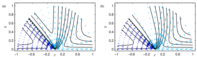
Figure 2: A comparison for a flow scenario in the intermediate region, governed by the Stokes equations, with $\Phi=3\pi/4$, $D_{A}=0.1$, $D_{B}=-0.1$, and $V_{c}=1$ for the two cases (a) $\mu_{B/A}=0$ and (b) $\mu_{B/A}=1$.

6 Contact line region

We now consider the inner region near to both interface and wall in polar coordinates with $r=O(\operatorname{Cn})$. The scaling $r=\operatorname{Cn}\tilde{r}$ (inner variables denoted with tildes) allows a balance that retains all terms in the governing equations and boundary conditions, giving a complete dominant balance. As such the contact line scalings are

$$r=\operatorname{Cn}\tilde{r},\quad\bm{\nabla}=\operatorname{Cn}^{-1}\tilde{\bm{\nabla}},\quad\rho=\tilde{\rho},\quad\textbf{u}=\tilde{\textbf{u}},\quad\textbf{u}_{w}=\tilde{\textbf{u}}_{w},$$

$$\textbf{M}=\operatorname{Cn}^{-1}\tilde{\textbf{M}},\quad\textbf{T}=\operatorname{Cn}^{-1}\tilde{\textbf{T}},\quad\bm{\tau}=\operatorname{Cn}^{-1}\tilde{\bm{\tau}},\quad p=\operatorname{Cn}^{-1}\tilde{p},$$ (114)

and variables are then expanded in the sharp-interface limit (for an arbitrary variable $\tilde{\phi}$) as

$$\tilde{\phi}=\tilde{\phi}^{(0)}+\operatorname{Cn}\tilde{\phi}^{(1)}+\operatorname{Cn}^{2}\tilde{\phi}^{(2)}+\ldots,$$ (115)

with the leading order terms being considered, and the superscript $(0)$ dropped for ease of exposition in what is to follow.

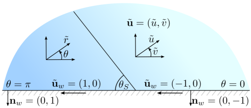
Figure 3: Sketch of the vicinity of the contact line in polar coordinates.

As the classical formulation of the problem analysed by Huh and Scriven⁷ predicted singularities in stress and pressure due to a multivalued velocity at the contact line, the behaviour as the contact line is approached in our diffuse-interface model is of particular interest. In this respect, we consider the (steady) continuity equation (23) and momentum equations (37), with boundary conditions (31) in polar coordinates, where $\tilde{u}$ and $\tilde{v}$ are the radial and angular velocity components (shown in Fig. 3), to obtain

$$\frac{\partial{}}{\partial{\tilde{r}}}(\tilde{\rho}\tilde{u})+\frac{\tilde{\rho}\tilde{u}}{\tilde{r}}+\frac{1}{\tilde{r}}\frac{\partial{}}{\partial{\tilde{\theta}}}(\tilde{\rho}\tilde{v}) =0,$$ (116)

$$\frac{1}{\operatorname{Ca}_{K}}\tilde{\rho}\left({\frac{\partial^{3}{\tilde{\rho}}}{\partial{\tilde{r}}^{3}}-\frac{1}{\tilde{r}^{2}}\frac{\partial{\tilde{\rho}}}{\partial{\tilde{r}}}+\frac{1}{\tilde{r}}\frac{\partial^{2}{\tilde{\rho}}}{\partial{\tilde{r}}^{2}}-\frac{2}{\tilde{r}^{3}}\frac{\partial^{2}{\tilde{\rho}}}{\partial{\tilde{\theta}}^{2}}+\frac{1}{\tilde{r}^{2}}\frac{\partial^{3}{\tilde{\rho}}}{\partial{\tilde{r}}\partial{\tilde{\theta}}^{2}}}\right)-\frac{1}{\operatorname{Ca}_{K}}\frac{\partial{}}{\partial{\tilde{r}}}\left({\tilde{\rho}^{2}f^{\prime}(\tilde{\rho})}\right)$$

$$+[2\mu(\tilde{\rho})+\nu(\tilde{\rho})]\left[{\frac{\partial^{2}{\tilde{u}}}{\partial{\tilde{r}}^{2}}+\frac{1}{\tilde{r}}\frac{\partial{\tilde{u}}}{\partial{\tilde{r}}}-\frac{\tilde{u}}{\tilde{r}^{2}}}\right]+\frac{\mu(\tilde{\rho})}{\tilde{r}^{2}}\frac{\partial^{2}{\tilde{u}}}{\partial{\tilde{\theta}}^{2}}-[3\mu(\tilde{\rho})+\nu(\tilde{\rho})]\frac{1}{\tilde{r}^{2}}\frac{\partial{\tilde{v}}}{\partial{\tilde{\theta}}}+[\mu(\tilde{\rho})+\nu(\tilde{\rho})]\frac{1}{\tilde{r}}\frac{\partial^{2}{\tilde{v}}}{\partial{\tilde{r}}\partial{\tilde{\theta}}}$$

$$+\left[{[2\mu^{\prime}(\tilde{\rho})+\nu^{\prime}(\tilde{\rho})]\frac{\partial{\tilde{u}}}{\partial{\tilde{r}}}+\nu^{\prime}(\tilde{\rho})\frac{1}{\tilde{r}}\left({\tilde{u}+\frac{\partial{\tilde{v}}}{\partial{\tilde{\theta}}}}\right)}\right]\frac{\partial{\tilde{\rho}}}{\partial{\tilde{r}}}+\mu^{\prime}(\tilde{\rho})\left[{\frac{1}{\tilde{r}^{2}}\frac{\partial{\tilde{u}}}{\partial{\tilde{\theta}}}-\frac{\tilde{v}}{\tilde{r}^{2}}+\frac{1}{\tilde{r}}\frac{\partial{\tilde{v}}}{\partial{\tilde{r}}}}\right]\frac{\partial{\tilde{\rho}}}{\partial{\tilde{\theta}}} =0,$$ (117)

$$\frac{1}{\operatorname{Ca}_{K}}\tilde{\rho}\frac{1}{\tilde{r}}\left({\frac{\partial^{3}{\tilde{\rho}}}{\partial{\tilde{r}}^{2}\partial{\tilde{\theta}}}+\frac{1}{\tilde{r}}\frac{\partial^{2}{\tilde{\rho}}}{\partial{\tilde{r}}\partial{\tilde{\theta}}}+\frac{1}{\tilde{r}^{2}}\frac{\partial^{3}{\tilde{\rho}}}{\partial{\tilde{\theta}}^{3}}}\right)-\frac{1}{\operatorname{Ca}_{K}}\frac{1}{\tilde{r}}\frac{\partial{}}{\partial{\tilde{\theta}}}\left({\tilde{\rho}^{2}f^{\prime}(\tilde{\rho})}\right)$$

$$+\mu(\tilde{\rho})\left[{\frac{\partial^{2}{\tilde{v}}}{\partial{\tilde{r}}^{2}}+\frac{1}{\tilde{r}}\frac{\partial{\tilde{v}}}{\partial{\tilde{r}}}-\frac{\tilde{v}}{\tilde{r}^{2}}}\right]+[2\mu(\tilde{\rho})+\nu(\tilde{\rho})]\frac{1}{\tilde{r}^{2}}\frac{\partial^{2}{\tilde{v}}}{\partial{\tilde{\theta}}^{2}}+[3\mu(\tilde{\rho})+\nu(\tilde{\rho})]\frac{1}{\tilde{r}^{2}}\frac{\partial{\tilde{u}}}{\partial{\tilde{\theta}}}+[\mu(\tilde{\rho})+\nu(\tilde{\rho})]\frac{1}{\tilde{r}}\frac{\partial^{2}{\tilde{u}}}{\partial{\tilde{r}}\partial{\tilde{\theta}}}$$

$$+\mu^{\prime}(\tilde{\rho})\left[{\frac{1}{\tilde{r}}\frac{\partial{\tilde{u}}}{\partial{\tilde{\theta}}}-\frac{\tilde{v}}{\tilde{r}}+\frac{\partial{\tilde{v}}}{\partial{\tilde{r}}}}\right]\frac{\partial{\tilde{\rho}}}{\partial{\tilde{r}}}+\left[{[2\mu^{\prime}(\tilde{\rho})+\nu^{\prime}(\tilde{\rho})]\frac{1}{\tilde{r}^{2}}\left({\tilde{u}+\frac{\partial{\tilde{v}}}{\partial{\tilde{\theta}}}}\right)+\nu^{\prime}(\tilde{\rho})\frac{1}{\tilde{r}}\frac{\partial{\tilde{u}}}{\partial{\tilde{r}}}}\right]\frac{\partial{\tilde{\rho}}}{\partial{\tilde{\theta}}} =0,$$ (118)

and the boundary conditions

$$\tilde{u} =-1, \tilde{v} =0, -\frac{\operatorname{Ca}}{6\operatorname{Ca}_{K}}\frac{1}{\tilde{r}}\frac{\partial{\tilde{\rho}}}{\partial{\theta}} =\cos\theta_{S}(1-\tilde{\rho})\tilde{\rho},\qquad \mbox{on }\theta=0,$$ (119)

$$\tilde{u} =1, \tilde{v} =0, \frac{\operatorname{Ca}}{6\operatorname{Ca}_{K}}\frac{1}{\tilde{r}}\frac{\partial{\tilde{\rho}}}{\partial{\theta}} =\cos\theta_{S}(1-\tilde{\rho})\tilde{\rho},\qquad \mbox{on }\theta=\pi.$$ (120)

Note that to transfer these polar velocity components to Cartesian, $\tilde{u}_{\textrm{Cartesian}}=\tilde{u}\cos\theta-\tilde{v}\sin\theta$, $\tilde{v}_{\textrm{Cartesian}}=\tilde{u}\sin\theta+\tilde{v}\cos\theta$. To consider the asymptotic solution as the contact line is approached, we consider the expansions

$$\tilde{\rho} =\tilde{\rho}_{0}(\theta)+\tilde{\rho}_{1}(\theta)\tilde{r}+\tilde{\rho}_{2}(\theta)\tilde{r}^{2}+\cdots,$$ (121)

$$\tilde{u} =\tilde{u}_{0}(\theta)+\tilde{u}_{1}(\theta)\tilde{r}+\tilde{u}_{2}(\theta)\tilde{r}^{2}+\cdots,$$ (122)

$$\tilde{v} =\tilde{v}_{0}(\theta)+\tilde{v}_{1}(\theta)\tilde{r}+\tilde{v}_{2}(\theta)\tilde{r}^{2}+\cdots.$$ (123)

At leading order we find

$$\tilde{u}_{0}=-\tilde{v}_{0}^{\prime}-\frac{\tilde{\rho}_{0}^{\prime}}{\tilde{\rho}_{0}}\tilde{v}_{0},\qquad\tilde{\rho}_{0}^{\prime\prime\prime}=0,\qquad\tilde{\rho}_{0}^{\prime\prime}=0,$$ (124)

subject to $\tilde{\rho}_{0}^{\prime}=0$ on $\theta=\{0,\pi\}$, $\tilde{u}_{0}=-1$, and $\tilde{v}_{0}=0$ on $\theta=0$, $\tilde{u}_{0}=1$, and $\tilde{v}_{0}=0$ on $\theta=\pi$. The general solution for the leading order density is of the form $\tilde{\rho}_{0}=C_{\tilde{\rho}_{1}}\tilde{\theta}+C_{\tilde{\rho}_{2}}$, and satisfying the wetting boundary condition at $O(r^{-1})$ forces $C_{\tilde{\rho}_{1}}=0$. Since the interface was defined at $\tilde{\rho}={1}/{2}$, we thus require $C_{\tilde{\rho}_{2}}={1}/{2}$, but leave it general to see its effect, and so that generalising to other definitions of interface could be considered. As we cannot solve for the velocities we continue to the following order and find

$$\tilde{u}_{0}=-\tilde{v}_{0}^{\prime},\qquad\mu(C_{\tilde{\rho}_{2}})\frac{\operatorname{Ca}_{K}}{C_{\tilde{\rho}_{2}}}(\tilde{v}_{0}^{\prime\prime\prime}+\tilde{v}_{0}^{\prime})+\tilde{\rho}_{1}^{\prime\prime}+\tilde{\rho}_{1}=0\qquad\mu(C_{\tilde{\rho}_{2}})\frac{\operatorname{Ca}_{K}}{C_{\tilde{\rho}_{2}}}(\tilde{v}_{0}^{\prime\prime}+\tilde{v}_{0})-\tilde{\rho}_{1}^{\prime\prime\prime}-\tilde{\rho}_{1}^{\prime}=0.$$ (125)

The general solution to these equations may be found to be

$$\tilde{\rho}_{1}=A_{\tilde{\rho}_{1}}\sin\theta+A_{\tilde{\rho}_{2}}\cos\theta+A_{\tilde{\rho}_{3}}\theta\sin\theta+A_{\tilde{\rho}_{4}}\theta\cos\theta,$$ (126)

$$\tilde{u}_{0}=\frac{C_{\tilde{\rho}_{2}}}{\mu(C_{\tilde{\rho}_{2}})\operatorname{Ca}_{K}}\left[{(A_{\tilde{\rho}_{4}}\theta+A_{\tilde{\rho}_{5}})\cos\theta+(A_{\tilde{\rho}_{3}}\theta+A_{\tilde{\rho}_{6}})\sin\theta}\right],$$ (127)

$$\tilde{v}_{0}=\frac{C_{\tilde{\rho}_{2}}}{\mu(C_{\tilde{\rho}_{2}})\operatorname{Ca}_{K}}\left[{(A_{\tilde{\rho}_{6}}-A_{\tilde{\rho}_{4}}+A_{\tilde{\rho}_{3}}\theta)\cos\theta-(A_{\tilde{\rho}_{5}}+A_{\tilde{\rho}_{3}}+A_{\tilde{\rho}_{4}}\theta)\sin\theta}\right].$$ (128)

The no-slip and wetting boundary conditions on $\theta=\{0,\pi\}$ are from (119)–(120). Using expansions (121)–(123), these are

$$\tilde{u}_{0}=\mp 1,\qquad\tilde{v}_{0}=0,\qquad\mp\frac{1}{6}\frac{\operatorname{Ca}}{\operatorname{Ca}_{K}}\tilde{\rho}_{1}^{\prime}=\cos(\theta_{S})C_{\tilde{\rho}_{2}}(1-C_{\tilde{\rho}_{2}}),$$ (129)

at $O(r^{0})$, which then give the density and velocity components as

$$\tilde{\rho}_{1}=\frac{6\operatorname{Ca}_{K}C_{\tilde{\rho}_{2}}(C_{\tilde{\rho}_{2}}-1)}{\operatorname{Ca}}\cos\theta_{S}\sin\theta+A_{\tilde{\rho}_{2}}\cos\theta,\qquad\tilde{u}_{0}=-\cos\theta,\qquad\tilde{v}_{0}=\sin\theta,$$ (130)

where $A_{\tilde{\rho}_{2}}$ is a constant of integration. If we assume that at these very small distances to the contact line the profile is planar (at the Young contact angle $\theta_{S}$), then we require $\tilde{\rho}(\tilde{r},\pi-\theta_{S})=C_{\tilde{\rho}_{2}}$ (or equivalently $\tilde{\rho}_{1}(\tilde{r},\pi-\theta_{S})=0$), at least up to this first order correction. As such

$$\frac{6\operatorname{Ca}_{K}C_{\tilde{\rho}_{2}}(C_{\tilde{\rho}_{2}}-1)}{\operatorname{Ca}}\cos\theta_{S}\sin(\pi-\theta_{S})+A_{\tilde{\rho}_{2}}\cos(\pi-\theta_{S})=0$$

$$\Rightarrow\qquad A_{\tilde{\rho}_{2}}=6\frac{\operatorname{Ca}_{K}}{\operatorname{Ca}}C_{\tilde{\rho}_{2}}\sin(\theta_{S})(C_{\tilde{\rho}_{2}}-1),$$ (131)

however, as with $C_{\tilde{\rho}_{2}}$, we will leave this general to see its effect. We now consider the stresses and pressure, scaled as in (114). The total stress components in polar coordinates and in inner variables are

$$\tilde{\textbf{M}}_{{\tilde{r}}{\tilde{r}}} =\frac{1}{\operatorname{Ca}_{K}}\left[\frac{1}{2}\left\{{2\tilde{\rho}f(\tilde{\rho})+\frac{1}{\tilde{r}^{2}}\left({\frac{\partial{\tilde{\rho}}}{\partial{\theta}}}\right)^{2}-\left({\frac{\partial{\tilde{\rho}}}{\partial{\tilde{r}}}}\right)^{2}}\right\}\right.$$

$$\left.+\tilde{\rho}\left\{{\frac{\partial^{2}{\tilde{\rho}}}{\partial{\tilde{r}}^{2}}+\frac{1}{\tilde{r}}\frac{\partial{\tilde{\rho}}}{\partial{r}}+\frac{1}{\tilde{r}^{2}}\frac{\partial^{2}{\tilde{\rho}}}{\partial{\theta}^{2}}-\frac{\partial{}}{\partial{\tilde{\rho}}}(\tilde{\rho}f(\tilde{\rho}))}\right\}\right]+[2\mu(\tilde{\rho})+\nu(\tilde{\rho})]\frac{\partial{\tilde{u}}}{\partial{\tilde{r}}}+\nu(\tilde{\rho})\frac{1}{\tilde{r}}\left({\tilde{u}+\frac{\partial{\tilde{v}}}{\partial{\theta}}}\right),$$ (132)

$$\tilde{\textbf{M}}_{\tilde{r}\theta} =-\frac{1}{\operatorname{Ca}_{K}}\frac{1}{\tilde{r}}\frac{\partial{\tilde{\rho}}}{\partial{\tilde{r}}}\frac{\partial{\tilde{\rho}}}{\partial{\theta}}+\mu(\tilde{\rho})\left[{\frac{1}{\tilde{r}}\left({\frac{\partial{\tilde{u}}}{\partial{\theta}}-\tilde{v}}\right)+\frac{\partial{\tilde{v}}}{\partial{\tilde{r}}}}\right],$$ (133)

$$\tilde{\textbf{M}}_{\theta\theta} =\frac{1}{\operatorname{Ca}_{K}}\left[\frac{1}{2}\left\{{2\tilde{\rho}f(\tilde{\rho})-\frac{1}{\tilde{r}^{2}}\left({\frac{\partial{\tilde{\rho}}}{\partial{\theta}}}\right)^{2}+\left({\frac{\partial{\tilde{\rho}}}{\partial{\tilde{r}}}}\right)^{2}}\right\}\right.$$

$$\left.+\tilde{\rho}\left\{{\frac{\partial^{2}{\tilde{\rho}}}{\partial{\tilde{r}}^{2}}+\frac{1}{\tilde{r}}\frac{\partial{\tilde{\rho}}}{\partial{r}}+\frac{1}{\tilde{r}^{2}}\frac{\partial^{2}{\tilde{\rho}}}{\partial{\theta}^{2}}-\frac{\partial{}}{\partial{\tilde{\rho}}}(\tilde{\rho}f(\tilde{\rho}))}\right\}\right]+\nu(\tilde{\rho})\frac{\partial{\tilde{u}}}{\partial{\tilde{r}}}+[2\mu(\tilde{\rho})+\nu(\tilde{\rho})]\frac{1}{\tilde{r}}\left({\tilde{u}+\frac{\partial{\tilde{v}}}{\partial{\theta}}}\right),$$ (134)

and we find at leading order $\tilde{\textbf{M}}=O(1)$, as all $O(1/\tilde{r})$ terms cancel. To obtain the precise form of the stresses, we require the second-order terms in the governing equations. The pressure in this inner region is of the form

$$\tilde{p}=\frac{1}{\operatorname{Ca}_{K}}\tilde{\rho}^{2}f^{\prime}(\tilde{\rho}),$$ (135)

and so at leading order as $\tilde{r}\to 0$, we find that $\tilde{p}={\operatorname{Ca}_{K}}^{-1}C_{\tilde{\rho}_{2}}^{2}f^{\prime}(C_{\tilde{\rho}_{2}})+O(\tilde{r})$, being finite at the contact line.

Continuing to find the second-order terms, we obtain the density and velocity corrections

$$\tilde{\rho}_{2} =D_{\tilde{\rho}_{1}}+D_{\tilde{\rho}_{2}}\cos(2\theta)+\frac{6\operatorname{Ca}_{K}}{\operatorname{Ca}}A_{\tilde{\rho}_{2}}\cos\theta_{S}(C_{\tilde{\rho}_{2}}-1/2)\sin(2\theta),$$ (136)

$$\left({\begin{array}[]{c}\tilde{u}_{1}\\ \tilde{v}_{1}\end{array}}\right) =\left({\begin{array}[]{c}\frac{A_{\tilde{\rho}_{2}}}{2C_{\tilde{\rho}_{2}}}(1-\cos(2\theta))-D_{\tilde{v}}\sin(2\theta)\\ \frac{A_{\tilde{\rho}_{2}}}{2C_{\tilde{\rho}_{2}}}\sin(2\theta)+D_{\tilde{v}}(1-\cos(2\theta))\end{array}}\right),$$ (141)

where the arbitrary constants $D_{\tilde{\rho}_{1}}$, $D_{\tilde{\rho}_{2}}$ and $D_{\tilde{v}}$ would be set by a full numerical solution of the contact line region. Using the results of the velocity, and converting into Cartesian components, we see that at the contact line

$$\tilde{u}_{\textrm{Cartesian}}=-1-2\tilde{y}D_{\tilde{v}}+\cdots,\qquad\tilde{v}_{\textrm{Cartesian}}=\frac{D_{\tilde{v}}}{C_{\tilde{\rho}_{2}}}\tilde{y}+\cdots,$$ (142)

showing the well-defined velocity approaching the contact line, at the wall $\tilde{y}=0$. All of these results allow us to determine the leading-order stress components as

$$\tilde{\textbf{M}}_{\tilde{r}\tilde{r}} =M_{1}\cos(2\theta)-M_{2}\sin(2\theta)+M_{3}+O(\tilde{r}),$$ (143)

$$\tilde{\textbf{M}}_{\tilde{r}\tilde{\theta}} =-M_{2}\cos(2\theta)-M_{1}\sin(2\theta)+O(\tilde{r}),$$ (144)

$$\tilde{\textbf{M}}_{\tilde{\theta}\tilde{\theta}} =M_{2}\sin(2\theta)-M_{1}\cos(2\theta)+M_{3}+O(\tilde{r}),$$ (145)

where

$$M_{1} =\frac{9\operatorname{Ca}_{K}(1-C_{\tilde{\rho}_{2}})^{2}C_{\tilde{\rho}_{2}}^{2}}{\operatorname{Ca}^{2}}(1+\cos(2\theta_{S}))-\frac{A_{\tilde{\rho}_{2}}}{C_{\tilde{\rho}_{2}}}\mu(C_{\tilde{\rho}_{2}})-\frac{1}{2\operatorname{Ca}_{K}}A_{\tilde{\rho}_{2}}^{2}$$ (146)

$$M_{2} =-6\frac{A_{\tilde{\rho}_{2}}C_{\tilde{\rho}_{2}}}{\operatorname{Ca}}\cos(\theta_{S})(1-C_{\tilde{\rho}_{2}})+2\mu(C_{\tilde{\rho}_{2}})C_{\tilde{v}},$$ (147)

$$M_{3} =\frac{A_{\tilde{\rho}_{2}}}{C_{\tilde{\rho}_{2}}}[\mu(C_{\tilde{\rho}_{2}})+\nu(C_{\tilde{\rho}_{2}})]-\frac{1}{\operatorname{Ca}_{K}}\left[{C_{\tilde{\rho}_{2}}^{2}f^{\prime}(C_{\tilde{\rho}_{2}})-4D_{\tilde{\rho}_{1}}C_{\tilde{\rho}_{2}}}\right],$$ (148)

showing that the stresses are nonsingular as $\tilde{r}\to 0$, as all $O(\tilde{r}^{-1})$ terms cancel.

Recall from Sec. 4 where we considered the sharp-interface limit away from the walls, that the (liquid-gas) interface gives rise to the classical boundary conditions (kinematic boundary condition, continuity of velocity, normal and tangential stress balances) in this limit, and that the two bulk phases satisfy the Navier–Stokes equations. This cannot be extended to the contact line region as the very reason that the diffuse-interface model resolves the moving contact line singularities is the diffuse nature (and finite thickness) of the interface. As already noted at the start of Sec. 6, the dominant balance of scalings for the contact line region shows that this region is of size $O(\operatorname{Cn})$, so the region where a diffuse-interface (i.e. not a sharp one) is significant is of this order (and as mentioned, all terms in the governing equations are retained). In fact the limit $\operatorname{Cn}\to 0$ is a singular perturbation problem, as setting $\operatorname{Cn}=0$ gives back the unsolvable classic problem (without any additional ingredients such as slip).

7 Conclusions

We have undertaken an analytical investigation of the contact line behaviour for a liquid-gas system with two basic elements: (a) the interface has a finite thickness, as expected from statistical mechanics studies, and (b) the no-slip condition is applied at the wall. The variation of the two viscosities between the liquid and gas phase have been left as general functions so as to be relevant to both equal (constant) viscosities, as considered by Seppecher,¹¹ and for disparate viscosities. The form of the double well contribution to the free energy has also been left general. In this case, our diffuse-interface model is then shown to resolve the singularities associated with the moving contact line problem without the need for any further physical effects from the microscale.

To summarize, our main results are:

• Determined the governing equations, identifying a suitable wall free energy form, in (11), to give a boundary condition to isolate the effect of the diffuse-interface on the contact line behaviour, without density gradients at the wall at large distances from the contact line.

• Considered a general viscosity relationship between the two fluid phases.

• Justified the model equations through considering the sharp-interface limit away from the contact line region, obtaining the classical bulk equations and interface conditions.

• Highlighted and corrected a discrepancy in the ‘intermediate region’ of the seminal work of Seppecher.¹¹

• Shown that the diffuse-interface model we adopted resolves the singularities associated with the moving contact line problem by considering the asymptotic behaviour in the vicinity of the contact line.

The model studied here imposed no-slip and enforced a wetting boundary condition causing the wall free energy to relax to equilibrium instantaneously. These conditions may be altered to allow for additional effects, if they are considered physically relevant, although doing so is not necessary to resolve the moving contact line problem, as determined in this study. Appropriate generalisations of the boundary conditions at the wall are to allow for finite-time relaxation, and to apply the generalised Navier boundary condition (GNBC) to allow for slip at the wall, these being discussed and derived by Qian, Wang, and Sheng,^{50, 49} Jacqmin,¹² and Yue and Feng,^{55, 24} for binary fluids. In dimensional form and for our liquid-gas configuration these are instead given by

$$\lambda\left({\partial_{\bar{t}}{\bar{\rho}}+\bar{\textbf{u}}\bm{\cdot}\bar{\bm{\nabla}}\bar{\rho}}\right)=-\bar{L}(\bar{\rho}),$$ (149)

where $\bar{L}(\bar{\rho})=K\textbf{n}_{w}\bm{\cdot}\bar{\bm{\nabla}}\bar{\rho}+\bar{f}^{\prime}_{w}(\bar{\rho})$ is the wall chemical potential, and with $\lambda=0$ representing instantaneous relaxation to equilibrium, and

$$\bar{L}(\bar{\rho})(\textbf{t}_{w}\bm{\cdot}\bar{\bm{\nabla}}\bar{\rho})-\bar{\bm{\tau}}_{nt}=\bar{\beta}(\bar{\textbf{u}}-\bar{\textbf{u}}_{w})\bm{\cdot}\textbf{t}_{w},$$ (150)

where $\bar{\beta}$ is the inverse slip length, $\textbf{t}_{w}$ the tangent to the wall, and $\bar{\bm{\tau}}_{nt}$ is the viscous shear stress. Note that $\lambda=0$ reduces to the popular Navier-slip condition. It is also of interest to note that such boundary conditions allow the diffuse-interface model to have a velocity dependent microscopic contact angle and to exhibit effective slip on the solid, both features of the continuum mechanical interface formation model of Shikhmurzaev²⁷ (and analysed in Ref. ⁵⁶).

The analysis presented here does not include boundary layers at the wall, which would arise if the wetting boundary condition is replaced by conditions such as (149), or a form to model a precursor film such as that used by Pismen and Pomeau³⁹, where $\bar{\rho}=\rho_{a}$, a constant, on $\partial\Omega$. This would be a rather involved problem to investigate using matched asymptotics, as the boundary layer at the wall would meet the boundary layer at the liquid-gas interface, and the two would need to match when “turning the corner” at the contact line, where the full inner equations should be retained, and most likely matching would have to be done numerically.

We believe that the present study will motivate further analytical and numerical work with diffuse-interface models, not just for ideally smooth substrates as was the case here but for (chemically or topographically) heterogeneous ones where previous studies have utilized a sharp-interface model with a slip boundary condition,^{57, 58, 59, 60, 61, 62} or have been numerically investigated with phase-field models.^{63, 64, 25} The binary fluid moving contact line problem (i.e. for a solid-liquid-liquid problem) is certainly of interest, but there remains ongoing debate on the correct scaling in the sharp-interface limit for an additional nondimensional “mobility” parameter, associated with the additional Cahn–Hilliard type equation for the order parameter.^{65, 18, 66, 67} There has, however, been some early progress in the work of Ref. ⁶⁸.

Additionally, the question of how diffuse-interface models may be adapted for non-Newtonian fluids is of interest. It is known that certain forms of shear-thinning non-Newtonian models are able to resolve the moving contact line problem without features like a diffuse-interface and whilst still applying no-slip,⁶⁹ however there are obviously a wealth of non-Newtonian behaviours other than shear-thinning which may be considered (for instance viscoelastic fluids, modelled with Maxwell or Oldroyd models). For an incompressible binary fluid model, a numerical investigation of an Oldroyd-B fluid in a Newtonian solvent has been studied, ⁷⁰ with the stress tensor of the Oldroyd-B fluid coupled into the total stress tensor. A possible extension to our analysis would be the consideration of a similar Oldroyd-B model, which would be in compressible form and coupled into our system of equations by replacing (5) in the manuscript by

$$\bar{\textbf{M}}=\bar{\textbf{T}}+\bar{\bm{\tau}}+\bar{\bm{\tau}}_{\textrm{poly}},\qquad\bar{\bm{\tau}}_{\textrm{e}}=\bar{\bm{\tau}}_{\textrm{poly}}+\bar{\nu}(\rho)[(\bar{\bm{\nabla}}\bm{\cdot}\bar{\textbf{u}})\textbf{I}],$$

$$\bar{\bm{\tau}}_{\textrm{e}}+\bar{\lambda}_{\textrm{e}}\stackrel{{\scriptstyle\triangledown}}{{\bar{\bm{\tau}}}}_{\textrm{e}}\ =\left[\bar{\mu}_{\textrm{e}}+\frac{\textrm{d}\bar{\mu}(\bar{\rho})}{\textrm{d}\bar{\rho}}\bar{\lambda}_{\textrm{e}}\,\bar{\rho}\,(\bar{\bm{\nabla}}\bm{\cdot}\bar{\textbf{u}})\right]\left[(\bar{\bm{\nabla}}\bar{\textbf{u}})+(\bar{\bm{\nabla}}\bar{\textbf{u}})^{\mathrm{T}}\right],$$ (151)

where $\bar{\bm{\tau}}_{\textrm{poly}}$ is the stress contribution from the polymer (so the usual Oldroyd stress tensor including polymer and solvent stresses is $\bm{\tau}_{o}=\bar{\bm{\tau}}+\bar{\bm{\tau}}_{\textrm{poly}}$), $\bar{\bm{\tau}}_{\textrm{e}}$ is a stress tensor chosen for convenience in writing the governing equations—effectively being $\bm{\tau}_{o}$ minus an incompressible Newtonian stress tensor, $\bar{\mu}_{\textrm{e}}$ is the polymer viscosity, and $\bar{\lambda}_{\textrm{e}}$ is the stress relaxation time (both of which could also be allowed to be density dependent in the above representation). These equations may be derived from equations (3), (7) and the usual Oldroyd-B model

$$\bm{\tau}_{o}+\bar{\lambda}_{\textrm{e}}\stackrel{{\scriptstyle\triangledown}}{{\bm{\tau}}}_{o}=2(\bar{\mu}_{\textrm{e}}+\bar{\mu})(\textbf{D}+\zeta_{o}\stackrel{{\scriptstyle\triangledown}}{{\textbf{D}}}),\qquad\textbf{D}=\left[(\bar{\bm{\nabla}}\bar{\textbf{u}})+(\bar{\bm{\nabla}}\bar{\textbf{u}})^{\mathrm{T}}\right]/2,$$ (152)

where $\zeta_{o}=\bar{\mu}\bar{\lambda}_{\textrm{e}}/(\bar{\mu}_{\textrm{e}}+\bar{\mu})$ is the retardation time of the Oldroyd-B model. Note here that the triangle denotes the upper convected stress derivative, defined for a general tensor $\bar{\textbf{A}}$ as

$$\stackrel{{\scriptstyle\triangledown}}{{\bar{\textbf{A}}}}=\frac{\partial\bar{\textbf{A}}}{\partial\bar{t}}+\bar{\textbf{u}}\bm{\cdot}\bar{\bm{\nabla}}\bar{\textbf{A}}-(\bar{\bm{\nabla}}\bar{\textbf{u}})\bar{\textbf{A}}-\bar{\textbf{A}}(\bar{\bm{\nabla}}\bar{\textbf{u}})^{\textrm{T}}.$$ (153)

Of particular interest for future work would also be the inclusion of non-local terms into the governing equations. This is considered for equilibrium wetting using a relatively simple density-functional formulation by Pereira and Kalliadasis,⁴³ capturing the non-local effects due to long-range intermolecular interactions. More involved density-functional theories, including inertial effects or hydrodynamic interactions, or both, are currently being pursued.^{71, 72, 73} The analysis here cannot be easily extended to include the relevant non-local terms, as dealing with integrals over the entire fluid volume in an asymptotic procedure (such as taking the sharp-interface limit) presents a highly nontrivial task.

Appendix A Square gradient approach from density functional theory

The diffuse-interface free energy in Eq. (1) may be derived through a Taylor series expansion of the density from a non-local model, which is also used in equilibrium density functional theory calculations, as suggested in Sec. 2. We give details here for the interested reader, noting that similar derivations are shown in Refs. ⁴⁸, ⁴², ⁴³.

In equilibrium density functional theory, the grand potential $\Omega^{\textrm{DFT}}$ of the system is given (e.g. see Refs. ¹⁹, ⁴³, ⁷⁴) by

$$\Omega^{\textrm{DFT}}[\bar{\rho}]=\int f_{\textrm{HS}}(\bar{\rho})\bar{\rho}(\bar{\textbf{r}})\textrm{d}\bar{\textbf{r}}+\frac{1}{2}\iint\bar{\rho}(\bar{\textbf{r}})\bar{\rho}(\bar{\textbf{r}}^{\prime})\phi_{\textrm{attr}}(\left|{\bar{\textbf{r}}-\bar{\textbf{r}}^{\prime}}\right|)\textrm{d}\bar{\textbf{r}}^{\prime}\textrm{d}\bar{\textbf{r}}+\int\bar{\rho}(\bar{\textbf{r}})(V_{p}(\bar{\textbf{r}})-\bar{G})\textrm{d}\bar{\textbf{r}},$$ (154)

where $\bar{\rho}(\bar{\textbf{r}})$ is the position dependent density, $f_{\textrm{HS}}(\bar{\rho})$ is the local hard sphere free energy, $V_{p}(\bar{\textbf{r}})$ is the non-local wall potential, and $\phi_{\textrm{attr}}(\left|{\bar{\textbf{r}}-\bar{\textbf{r}}^{\prime}}\right|)$ is the interaction potential between two particles. This grand potential uses a local density approximation (LDA) for hard-sphere interactions, with a mean-field theory for the attractive perturbation modelled using the Barker and Henderson approach:⁷⁵

$$\phi_{\textrm{attr}}(\bar{r})=\left\{\begin{array}[]{ll}0&\bar{r}\leq\hat{\sigma}\\ 4\hat{\epsilon}\left[{\left({\frac{\hat{\sigma}}{\bar{r}}}\right)^{12}-\left({\frac{\hat{\sigma}}{\bar{r}}}\right)^{6}}\right]&\bar{r}>\hat{\sigma}\end{array}\right.,$$ (157)

where $\hat{\sigma}$ is the soft-core parameter of the Lennard-Jones potential of the fluid-fluid interaction, and $\hat{\epsilon}$ is a parameter that measures the strength of the potential. At equilibrium, the grand potential is minimised:

$$\frac{\delta\Omega^{\textrm{DFT}}[\bar{\rho}]}{\delta\bar{\rho}(\bar{\textbf{r}})}=0,\qquad\mbox{giving}\qquad\frac{\partial{}}{\partial{\bar{\rho}}}(\bar{\rho}f_{\textrm{HS}}(\bar{\rho}))+\int\bar{\rho}(\bar{\textbf{r}}^{\prime})\phi_{\textrm{attr}}(\left|{\bar{\textbf{r}}-\bar{\textbf{r}}^{\prime}}\right|)\textrm{d}\bar{\textbf{r}}^{\prime}+V_{p}(\bar{\textbf{r}})=\bar{G},$$ (158)

the non-locality involving the interaction potential being clear. Obtaining the square gradient approximation, a Taylor series expansion of $\bar{\rho}(\bar{\textbf{r}})$ gives

$$\bar{\mathscr{F}}[\bar{\rho}]=\int(f_{\textrm{HS}}(\bar{\rho})-\bar{G}-\alpha\bar{\rho}(\bar{\textbf{r}}))\bar{\rho}(\bar{\textbf{r}})\textrm{d}\bar{\textbf{r}}+\int\frac{K}{2}\left|{\bar{\bm{\nabla}}\bar{\rho}(\bar{\textbf{r}})}\right|^{2}\textrm{d}\bar{\textbf{r}}+\int\bar{f}_{w}(\bar{\rho})\textrm{d}A,$$ (159)

neglecting terms of the third derivative and higher, and thus assuming the density of the fluid varies slowly, as for instance a fluid near its critical point. The non-local wall potential $V_{p}(\bar{\textbf{r}})$ has been replaced by a wall free energy $\bar{f}_{w}(\bar{\rho})$ on the substrate, and coefficients $K$ and $\alpha$ are given by

$$K=-\frac{2\pi}{3}\int\bar{r}^{4}\phi_{\textrm{attr}}(\bar{r})\textrm{d}\bar{r}=\frac{9}{7}\alpha\hat{\sigma}^{2},\qquad\mbox{and}\qquad\alpha=-\frac{1}{2}\iiint\phi_{\textrm{attr}}(\left|{\bar{\textbf{r}}}\right|)\textrm{d}\bar{\textbf{r}}=\frac{16}{9}\pi\hat{\epsilon}\hat{\sigma}^{3}.$$ (160)

By writing $\bar{f}(\bar{\rho})=f_{\textrm{HS}}(\bar{\rho})-\alpha\bar{\rho}(\bar{\textbf{r}})$, the free energy in (159) then reduces to that of the diffuse-interface model in Eq. (1).

Appendix B Body fitted coordinates

In Sec. 4.2 we utilize body fitted coordinates $(\xi,\eta)$ (as, for example in Refs. ⁷⁶, ⁷⁷, ⁷⁸, ⁷⁹, ⁸⁰) to the interface (given by $\textbf{r}=\textbf{r}_{0}(\xi,t)$, where r is any arbitrary point). $\xi$ measures distance along the interface (like an arc length), and $\eta$ measures the distance in the normal direction from the point $(x,y)\in\Omega$ to the interface $\Gamma=\Gamma(t)$. We note that these coordinates will only be valid locally in $\eta$, i.e. near the interface, as $\eta$ can become singular for a curved interface, as it reaches the radius of curvature. For slowly moving contact line problems the distortion of the interface will be small and no issues will arise. From our definition of the coordinates, we have

$$\textbf{r}=\textbf{r}_{0}(\xi,t)+\eta\textbf{n},$$ (161)

where n is the unit normal to the interface (noting that $\textbf{n}=\bm{\nabla}\eta$). As r is an arbitrary point, then the conversion between Cartesian and body fitted coordinates follows

$$\textbf{r}=x\textbf{i}+y\textbf{j}=\xi\textbf{e}_{1}+\eta\textbf{e}_{2},$$

$$\textbf{e}_{1}=\frac{\partial{x}}{\partial{\xi}}\textbf{i}+\frac{\partial{y}}{\partial{\xi}}\textbf{j},$$

$$\textbf{e}_{2}=\frac{\partial{x}}{\partial{\eta}}\textbf{i}+\frac{\partial{y}}{\partial{\eta}}\textbf{j}.$$ (162)

We define $\alpha$ as the angle from i to $\textbf{e}_{1}$, so that the curvature $\kappa=\partial_{\xi}{\alpha}$. At $\textbf{r}_{0}$ on the interface we have $X$ and $Y$ being the specific values of $x$ and $y$ (i.e. at a specific $\xi$). Moving a small amount $d\xi$ along the interface gives $d\xi\cos\alpha=dX$ and $d\xi\sin\alpha=dY$. Now consider $(x,y)$ being a point not on the interface, and at a signed distance $\eta$ away. Then we have $x=X-\eta\sin\alpha$ and $y=Y+\eta\cos\alpha$. Returning to (162) we find

$$\textbf{e}_{1} =\left(\frac{\partial{X}}{\partial{\xi}}-\eta\cos\alpha\frac{\partial{\alpha}}{\partial{\xi}}\right)\textbf{i}+\left(\frac{\partial{Y}}{\partial{\xi}}-\eta\sin\alpha\frac{\partial{\alpha}}{\partial{\xi}}\right)\textbf{j}=(1-\kappa\eta)(\cos\alpha\textbf{i}+\sin\alpha\textbf{j})$$

$$=(1-\kappa\eta)\textbf{t},$$ (163)

$$\textbf{e}_{2} =\left(\frac{\partial{X}}{\partial{\eta}}-\sin\alpha\right)\textbf{i}+\left(\frac{\partial{Y}}{\partial{\eta}}+\cos\alpha\right)\textbf{j}=-\sin\alpha\textbf{i}+\cos\alpha\textbf{j}$$

$$=\textbf{n},$$ (164)

giving the basis vectors for the body fitted coordinates, where t is the unit tangent to the interface.

The components of the metric tensor of these curvilinear coordinates are used to determine operators such as the gradient and Laplacian in these coordinates, and are found through $g_{ij}=\textbf{e}_{i}\bm{\cdot}\textbf{e}_{j}$. For orthogonal curvilinear coordinates (such as we have here) we also have $\textbf{e}^{1}=g^{11}\textbf{e}_{1}+g^{12}\textbf{e}_{2}$, $\textbf{e}^{2}=g^{12}\textbf{e}_{1}+g^{22}\textbf{e}_{2}$ and $g^{11}=1/g_{11}$, $g^{22}=1/g_{22}$, $g^{12}=g_{12}=0$, thus

$$g_{11}=(1-\kappa\eta)^{2},\quad g_{12}=0,\quad g_{22}=1,\mbox{ and }g^{11}=(1-\kappa\eta)^{-2},\quad g^{12}=0,\quad g^{22}=1.$$ (165)

Having this information, we are now able to determine the relevant terms in the governing equations. Time derivatives satisfy

$$\frac{\partial{}}{\partial{t}}\rho(x,y,t)=\frac{\partial{}}{\partial{t}}{\rho}(\xi,\eta,t)+\textbf{u}^{s}\bm{\cdot}\bm{\nabla}{\rho}(\xi,\eta,t)$$ (166)

where $\textbf{u}^{s}=(\partial_{t}{\xi},\partial_{t}{\eta})$ is the interface velocity, showing that the time derivative in the comoving frame is a material derivative. Considering $\textbf{u}=({u},v)$, and writing $h=\sqrt{g_{11}g_{22}}$ for convenience, then

$$\bm{\nabla}\rho =\frac{\partial{\rho}}{\partial{\xi}}\textbf{e}^{1}+\frac{\partial{\rho}}{\partial{\eta}}\textbf{e}^{2}=(1-\kappa\eta)^{-2}\frac{\partial{\rho}}{\partial{\xi}}\textbf{e}_{1}+\frac{\partial{\rho}}{\partial{\eta}}\textbf{e}_{2},$$ (167)

$$|\bm{\nabla}\rho|^{2} =(1-\kappa\eta)^{-2}\left(\frac{\partial{\rho}}{\partial{\xi}}\right)^{2}+\left(\frac{\partial{\rho}}{\partial{\eta}}\right)^{2},$$ (168)

$$\bm{\nabla}\bm{\cdot}\textbf{u} =\frac{1}{h}\left[\frac{\partial{}}{\partial{\xi}}\left(h{u}\right)+\frac{\partial{}}{\partial{\eta}}\left(hv\right)\right]=\frac{\partial{v}}{\partial{\eta}}-\frac{\kappa v}{1-\kappa\eta}+\frac{\partial{{u}}}{\partial{\xi}}-\frac{{u}\eta}{1-\kappa\eta}\frac{\partial{\kappa}}{\partial{\xi}},$$ (169)

$$\nabla^{2}\rho =\frac{1}{h}\left[\frac{\partial{}}{\partial{\xi}}\left(\frac{h}{g_{11}}\frac{\partial{\rho}}{\partial{\xi}}\right)+\frac{\partial{}}{\partial{\eta}}\left(\frac{h}{g_{22}}\frac{\partial{\rho}}{\partial{\eta}}\right)\right]$$

$$=\frac{1}{(1-\kappa\eta)^{2}}\frac{\partial^{2}{\rho}}{\partial{\xi}^{2}}+\frac{\eta\partial_{\xi}{\kappa}}{(1-\kappa\eta)^{3}}\frac{\partial{\rho}}{\partial{\xi}}+\frac{\partial^{2}{\rho}}{\partial{\eta}^{2}}-\frac{\kappa}{1-\kappa\eta}\frac{\partial{\rho}}{\partial{\eta}}.$$ (170)

For certain matrix quantities the Christoffel symbols of the second kind will be required, which are defined as

$$\Gamma_{ij}^{k}=\frac{g^{km}}{2}\left(\frac{\partial{g_{mi}}}{\partial{\chi_{j}}}+\frac{\partial{g_{mj}}}{\partial{\chi_{i}}}+\frac{\partial{g_{ij}}}{\partial{\chi_{m}}}\right),$$ (171)

where $\chi_{1}=\xi$ and $\chi_{2}=\eta$, so that

$$\Gamma_{11}^{1}=-\frac{\eta}{1-\kappa\eta}\frac{\partial{\kappa}}{\partial{\xi}},\quad\Gamma_{12}^{1}=\Gamma_{21}^{1}=-\frac{\kappa}{1-\kappa\eta},\quad\Gamma_{11}^{2}=\frac{\kappa}{1-\kappa\eta},\quad\mbox{and}\quad\Gamma_{ij}^{k}=0\mbox{ otherwise}.$$ (172)

We may then determine

I $$=\textbf{e}^{1}\otimes\textbf{e}_{2}+\textbf{e}^{2}\otimes\textbf{e}_{1}=\left(\begin{array}[]{cc}(1-\kappa\eta)^{-2}&0\\ 0&1\end{array}\right),$$ (175)

$$\nabla\rho\otimes\nabla\rho =\left(\begin{array}[]{cc}\left[(1-\kappa\eta)^{-2}\partial_{\xi}{\rho}\right]^{2}&(1-\kappa\eta)^{-2}(\partial_{\xi}{\rho})(\partial_{\eta}{\rho})\\ (1-\kappa\eta)^{-2}(\partial_{\xi}{\rho})(\partial_{\eta}{\rho})&\left(\partial_{\eta}{\rho}\right)^{2}\end{array}\right),$$ (178)

$$\bm{\nabla}\textbf{u} =\left(\frac{\partial{u_{i}}}{\partial{\chi_{k}}}+\Gamma^{i}_{lk}u_{l}\right)\textbf{e}_{i}\otimes\textbf{e}^{k}$$

$$=\left(\begin{array}[]{cc}\partial_{\xi}{{u}}-\eta(\partial_{\xi}{\kappa})(1-\kappa\eta)^{-1}{u}-\kappa(1-\kappa\eta)^{-1}v&\partial_{\eta}{u}-\kappa(1-\kappa\eta){u}\\ \partial_{\xi}{v}+\kappa(1-\kappa\eta){u}&\partial_{\eta}{v}\end{array}\right),$$ (181)

where $(u_{1},u_{2})=(u,v)$, and leading to the components of the viscous stress tensor being

$$(\bm{\tau})_{11} =\left(\frac{\partial{{u}}}{\partial{\xi}}-\frac{\kappa v}{1-\kappa\eta}-\frac{\eta{u}}{1-\kappa\eta}\frac{\partial{\kappa}}{\partial{\xi}}\right)\left(2\mu(\rho)+\nu(\rho)(1-\kappa\eta)^{-2}\right)+\nu(\rho)(1-\kappa\eta)^{-2}\frac{\partial{v}}{\partial{\eta}}$$

$$(\bm{\tau})_{12} =\mu(\rho)\left[{\frac{\partial{{u}}}{\partial{\eta}}+\frac{\partial{v}}{\partial{\xi}}}\right]$$

$$(\bm{\tau})_{22} =\left({2\mu(\rho)+\nu(\rho)}\right)\frac{\partial{v}}{\partial{\eta}}+\nu(\rho)\left(\frac{\partial{{u}}}{\partial{\xi}}-\frac{\kappa v}{1-\kappa\eta}-\frac{\eta{u}}{1-\kappa\eta}\frac{\partial{\kappa}}{\partial{\xi}}\right),$$ (182)

and the divergence of our (symmetric) total stress tensor M is

$$\bm{\nabla}\bm{\cdot}\textbf{M}=\left(\begin{array}[]{c}\partial_{\xi}{[(\textbf{M})_{11}]}+\partial_{\eta}{[(\textbf{M})_{12}]}+2\Gamma_{11}^{1}(\textbf{M})_{11}+3\Gamma_{12}^{1}(\textbf{M})_{12}\\ \partial_{\xi}{[(\textbf{M})_{12}]}+\partial_{\eta}{[(\textbf{M})_{22}]}+\Gamma_{11}^{1}(\textbf{M})_{12}+\Gamma_{12}^{1}(\textbf{M})_{22}+\Gamma_{11}^{2}(\textbf{M})_{11}\end{array}\right).$$ (185)

Appendix C Coefficients for the Seppecher intermediate solution

The intermediate solution of Seppecher was discussed in Sec. 5. The coefficients of the solutions of that section are for $V_{c}=0$:

$$C_{0,A} =\frac{\cos\Phi}{D_{D0}}\left[{(D_{A}-D_{B})\sin^{2}\Phi-2\pi\Phi D_{A}\cos(2\Phi)}\right](1-\mu_{B/A})$$

$$+\frac{\sin\Phi}{D_{D0}}\left[{2(\pi-\Phi)D_{A}\cos^{2}\Phi+(D_{A}+D_{B})\Phi-\pi D_{B}\cos(2\Phi)}\right](1-\mu_{B/A})$$

$$+\frac{\sin\Phi}{D_{D0}}\left[{(D_{A}+D_{B})(\cos\Phi\sin\Phi-2\pi\sin^{2}\Phi-\Phi)+\pi D_{B}}\right],$$ (186)

$$C_{1,A} =\frac{2N_{D0}}{D_{D0}},$$ (187)

$$C_{2,A} =-\frac{N_{D0}}{D_{D0}},$$ (188)

$$C_{3,A} =\frac{1}{D_{D0}\sin\Phi}\left[{(\Phi\cos(2\Phi)-\cos\Phi\sin\Phi)D_{A}-(\Phi-\pi)\sin^{2}\Phi D_{B}}\right](1-\mu_{B/A})$$

$$-\frac{1}{D_{D0}\sin\Phi}\left[{N_{D0}\cos\Phi-\sin^{2}\Phi\left({(D_{A}+D_{B})\Phi-\pi D_{B}}\right)}\right],$$

and

$$C_{0,B} =-\frac{[(\pi-\Phi)\cos\Phi+\sin\Phi]D_{B}\sin(2\Phi)(1-\mu_{B/A})}{D_{D0}}$$

$$-\frac{D_{A}\Phi-(D_{A}+D_{B})\sin\Phi\cos\Phi+(\Phi-\pi)D_{B}}{D_{D0}}\sin\Phi,$$ (190)

$$C_{1,B} =2{\frac{\left[(\pi-\Phi)\cos\Phi+\sin\Phi\right]\cos(2\Phi)D_{B}(1-\mu_{B/A})+\sin^{3}\Phi(D_{A}+D_{B})}{D_{D0}}},$$ (191)

$$C_{2,B} =-\frac{1}{2}C_{1,B},$$ (192)

$$C_{3,B} =-C_{0,B},$$ (193)

where

$$N_{D0} =\left\{D_{A}\left[\Phi\cos\Phi\cos(2\Phi)-\sin\Phi\right]+\sin^{3}\Phi(D_{A}-D_{B})\right\}(1-\mu_{B/A})+\sin^{3}\Phi(D_{A}+D_{B}),$$ (194)

$$D_{D0} =\cos\Phi\left[2\Phi\left\{{(\Phi-\pi)\cos(2\Phi)+\tan\Phi}\right\}+(\pi-3\Phi)\sin(2\Phi)+2\sin^{2}\Phi\right](1-\mu_{B/A})-2\pi\sin^{3}\Phi.$$ (195)

For $D_{A,B}=0$ the coefficients are:

$$k_{0,A} =-V_{c}-\pi k_{2,A}+k_{1,A}/\pi,$$ (196)

$$k_{1,A} =V_{c}\pi\sin\Phi\cos\Phi\frac{\mu_{B/A}(\sin^{2}\Phi-(\Phi-\pi)\Phi-\pi\tan\Phi)+\Phi^{2}-\sin^{2}\Phi}{D_{V0}},$$ (197)

$$k_{2,A} =V_{c}\sin^{2}\Phi\frac{-\mu_{B/A}(\sin^{2}\Phi-\Phi^{2}+\pi\Phi)-\Phi^{2}+\sin^{2}\Phi}{D_{V0}},$$ (198)

$$k_{3,A} =-\frac{k_{1,A}}{\pi},$$ (199)

and

$$k_{0,B} =-V_{c}-k_{3,B},$$ (200)

$$k_{1,B} =0,$$ (201)

$$k_{2,B} =-V_{c}\sin^{2}\Phi\frac{\mu_{B/A}(\sin^{2}\Phi-(\Phi-\pi)^{2})+(\Phi-\pi)\Phi-\sin^{2}\Phi}{D_{V0}},$$ (202)

$$k_{3,B} =-V_{c}\sin\Phi\cos\Phi\frac{\mu_{B/A}(\sin^{2}\Phi-(\Phi-\pi)^{2})+(\Phi-\pi)\Phi-\sin^{2}\Phi-\pi\tan\Phi}{D_{V0}},$$ (203)

where

$$D_{V0} =\mu_{B/A}(\sin^{2}\Phi-(\pi-\Phi)^{2})(\cos\Phi\sin\Phi-\Phi)+(\sin^{2}\Phi-\Phi^{2})(\Phi-\pi-\cos\Phi\sin\Phi).$$ (204)

For the specific case considered by Seppecher,¹¹ where $\mu_{B/A}=1$, these substantially simplify. For $V_{c}=0$, the solutions are

$$\Psi_{A}\left({\theta}\right) =\frac{D_{A}+D_{B}}{\pi}\left({\pi-\theta+\frac{\sin\theta}{\sin\Phi}\sin\left({\Phi-\theta}\right)+\Phi\frac{\sin^{2}\theta}{\sin^{2}\Phi}}\right)-D_{B}\frac{\sin^{2}\theta}{\sin^{2}\Phi},$$ (205)

$$\Psi_{B}\left({\theta}\right) =\Psi_{A}\left({\theta}\right)-\left({D_{A}+D_{B}}\right),$$ (206)

and for $D_{A,B}=0$ they are

$$\Psi_{A}\left({r,\theta}\right) =\frac{rV_{c}}{C}\left\{a_{1}(\theta-\pi)\sin\left({\theta-\Phi}\right)+a_{2}\left({\theta-\Phi}\right)\sin\theta\right\},$$ (207)

$$\Psi_{B}\left({r,\theta}\right) =\frac{rV_{c}}{C}\left\{b_{1}\theta\sin(\theta-\Phi)+b_{2}\left({\theta-\Phi}\right)\sin\theta\right\},$$ (208)

where

$$C =\Phi\left({\pi-\Phi}\right)-\sin^{2}\Phi+\left({2\Phi-\pi}\right)\cos\Phi\sin\Phi,$$ (209)

$$a_{1} =\Phi\cos\Phi-\sin\Phi,$$ (210)

$$a_{2} =\cos\Phi\sin\Phi-\Phi,$$ (211)

$$b_{1} =\left({\Phi-\pi}\right)\cos\Phi-\sin\Phi,$$ (212)

$$b_{2} =\cos\Phi\sin\Phi+\pi-\Phi.$$ (213)

We note that the specific forms of these solutions in Ref. ¹¹ have minor typographical errors (separate from the discussions in Sec. 5), so will not agree directly with our solutions above.

References

- 1 E. B. Dussan V. On the spreading of liquids on solid surfaces: Static and dynamic contact lines. Annu. Rev. Fluid Mech., 11(1):371–400, 1979.
- 2 P. G. de Gennes. Wetting: statics and dynamics. Rev. Mod. Phys., 57:827–863, 1985.
- 3 T. Blake. The physics of moving wetting lines. J. Colloid Interface Sci., 299(1):1–13, 2006.
- 4 D. Bonn, J. Eggers, J. Indekeu, J. Meunier, and E. Rolley. Wetting and spreading. Rev. Mod. Phys., 81:739–805, 2009.
- 5 E. B. Dussan V. and S. H. Davis. On the motion of a fluid-fluid interface along a solid surface. J. Fluid Mech., 65(1):71–95, 1974.
- 6 Y. D. Shikhmurzaev. Singularities at the moving contact line. Mathematical, physical and computational aspects. Physica D, 217(2):121–133, 2006.
- 7 C. Huh and L. E. Scriven. Hydrodynamic model of steady movement of a solid / liquid / fluid contact line. J. Colloid Interface Sci., 35(1):85–101, 1971.
- 8 C.-L. Navier. Mémoire sur les lois du mouvement des fluides. Mem. Acad. Sci. Inst. Fr., 6:389–440, 1823.
- 9 N. Savva and S. Kalliadasis. Dynamics of moving contact lines: A comparison between slip and precursor film models. Europhys. Lett., 94(6):64004, 2011.
- 10 D. M. Anderson, G. B. McFadden, and A. A. Wheeler. Diffuse-interface methods in fluid mechanics. Annu. Rev. Fluid Mech., 30:139–165, 1998.
- 11 P. Seppecher. Moving contact lines in the Cahn-Hilliard theory. Int. J. Eng. Sci., 34(9):977–992, 1996.
- 12 D. Jacqmin. Contact-line dynamics of a diffuse fluid interface. J. Fluid Mech., 402:57–88, 2000.
- 13 A. Briant. Lattice Boltzmann simulations of contact line motion in a liquid-gas system. Philos. T. Roy. Soc. A, 360(1792):485–495, 2002.
- 14 A. J. Briant, A. J. Wagner, and J. M. Yeomans. Lattice Boltzmann simulations of contact line motion. I. Liquid-gas systems. Phys. Rev. E, 69:031602, 2004.
- 15 D. Jasnow and J. Viñals. Coarse-grained description of thermo-capillary flow. Phys. Fluids, 8(3):660–669, 1996.
- 16 V. V. Khatavkar, P. D. Anderson, and H. E. H. Meijer. Capillary spreading of a droplet in the partially wetting regime using a diffuse-interface model. J. Fluid Mech., 572:367–387, 2007.
- 17 H. Ding and P. D. M. Spelt. Inertial effects in droplet spreading: a comparison between diffuse-interface and level-set simulations. J. Fluid Mech., 576:287–296, 2007.
- 18 P. Yue, C. Zhou, and J. J. Feng. Sharp-interface limit of the Cahn–Hilliard model for moving contact lines. J. Fluid Mech., 645:279–294, 2010.
- 19 R. Evans. The nature of the liquid-vapour interface and other topics in the statistical mechanics of non-uniform, classical fluids. Adv. Phys., 28(2):143–200, 1979.
- 20 D. Henderson. Fundamentals of Inhomogeneous Fluids. Dekker, New York, 1st. edition, 1992.
- 21 A. Nold, A. Malijevský, and S. Kalliadasis. Wetting on a spherical wall: Influence of liquid-gas interfacial properties. Phys. Rev. E, 84:021603, 2011.
- 22 P. Yatsyshin, N. Savva, and S. Kalliadasis. Spectral methods for the equations of classical density-functional theory: Relaxation dynamics of microscopic films. J. Chem. Phys., 136(12):124113, 2012.
- 23 N. D. Alikakos, P. W. Bates, and X. Chen. Convergence of the Cahn–Hilliard equation to the Hele–Shaw model. Arch. Rational Mech. Anal., 128(2):165–205, 1994.
- 24 P. Yue and J. J. Feng. Wall energy relaxation in the Cahn–Hilliard model for moving contact lines. Phys. Fluids, 23(1):012106, 2011.
- 25 C. Wylock, M. Pradas, B. Haut, P. Colinet, and S. Kalliadasis. Disorder-induced hysteresis and nonlocality of contact line motion in chemically heterogeneous microchannels. Phys. Fluids, 24(3):032108, 2012.
- 26 M. G. Velarde. Discussion and Debate: Wetting and Spreading Science - quo vadis? [Special issue]. Eur. Phys. J. Special Topics, 197:1–2, 2011.
- 27 Y. D. Shikhmurzaev. Capillary Flows with Forming Interfaces. Taylor & Francis, London, 2008.
- 28 Y. D. Shikhmurzaev. Some dry facts about dynamic wetting. Eur. Phys. J. Special Topics, 197:47–60, 2011.
- 29 Y. D. Shikhmurzaev. Discussion notes. Eur. Phys. J. Special Topics, 197:73–74, 2011.
- 30 Y. D. Shikhmurzaev. Discussion Notes on “Some singular errors near the contact line singularity, and ways to resolve both”, by L.M. Pismen. Eur. Phys. J. Special Topics, 197:75–80, 2011.
- 31 Y. D. Shikhmurzaev. Discussion Notes: On capillarity and slightly beyond. Eur. Phys. J. Special Topics, 197:85–87, 2011.
- 32 Y. D. Shikhmurzaev. Discussion Notes on “Note on thin film equations for solutions and suspensions”, by U. Thiele. Eur. Phys. J. Special Topics, 197:221–225, 2011.
- 33 U. Thiele. Discussion Notes: Thoughts on mesoscopic continuum models. Eur. Phys. J. Special Topics, 197:67–71, 2011.
- 34 L. M. Pismen. Some singular errors near the contact line singularity, and ways to resolve both. Eur. Phys. J. Special Topics, 197:33–36, 2011.
- 35 L. M. Pismen. Discussion Notes on “Some dry facts about dynamic wetting”, by Y.D. Shikhmurzaev. Eur. Phys. J. Special Topics, 197:63–65, 2011.
- 36 Y. Pomeau. Discussion Notes: More (and last remarks) on the debate on capillarity. Eur. Phys. J. Special Topics, 197:81–83, 2011.
- 37 Y. Pomeau. Discussion notes: Phase field models and moving contact line in the long perspective. Eur. Phys. J. Special Topics, 197(1):11–13, 2011.
- 38 T. D. Blake. Discussion notes: A more collaborative approach to the moving contact-line problem? Eur. Phys. J. Special Topics, 197:343–345, 2011.
- 39 L. M. Pismen and Y. Pomeau. Disjoining potential and spreading of thin liquid layers in the diffuse-interface model coupled to hydrodynamics. Phys. Rev. E, 62:2480–2492, 2000.
- 40 D. N. Sibley, A. Nold, N. Savva, and S. Kalliadasis. On the moving contact line singularity: Asymptotics of a diffuse-interface model. Eur. Phys. J. E, 36:26, 2013.
- 41 J. W. Cahn. Critical point wetting. J. Chem. Phys., 66(8):3667–3672, 1977.
- 42 L. Pismen. Mesoscopic hydrodynamics of contact line motion. Colloid. Surface. A, 206(1–3):11 – 30, 2002.
- 43 A. Pereira and S. Kalliadasis. Equilibrium gas–-liquid–-solid contact angle from density-functional theory. J. Fluid Mech., 692:53–77, 2012.
- 44 E. Noether. Invariante variationsprobleme. Nachr. v. d. Ges. d. Wiss. zu Göttingen, pages 235–257, 1918.
- 45 M. Schmuck, M. Pradas, G. A. Pavliotis, and S. Kalliadasis. Upscaled phase-field models for interfacial dynamics in strongly heterogeneous domains. Proc. R. Soc. A, 468(2147):3705–3724, 2012.
- 46 P. Yue, J. J. Feng, C. Liu, and J. Shen. A diffuse-interface method for simulating two-phase flows of complex fluids. J. Fluid Mech., 515:293–317, 2004.
- 47 X. Xu and T. Qian. Contact line motion in confined liquid–gas systems: Slip versus phase transition. J. Chem. Phys., 133(20):204704, 2010.
- 48 J. W. Cahn and J. E. Hilliard. Free energy of a nonuniform system. I. Interfacial free energy. J. Chem. Phys., 28(2):258–267, 1958.
- 49 T. Qian, X.-P. Wang, and P. Sheng. A variational approach to moving contact line hydrodynamics. J. Fluid Mech., 564:333–360, 2006.
- 50 T. Qian, X.-P. Wang, and P. Sheng. Molecular scale contact line hydrodynamics of immiscible flows. Phys. Rev. E, 68:016306, 2003.
- 51 C. Gugenberger, R. Spatschek, and K. Kassner. Comparison of phase-field models for surface diffusion. Phys. Rev. E, 78:016703, 2008.
- 52 G. K. Batchelor. An Introduction to Fluid Dynamics. Cambridge University Press, Cambridge, 2000.
- 53 I. Fredholm. Sur une classe d’équations fonctionnelles. Acta Mathematica, 27:365–390, 1903.
- 54 H. K. Moffatt. Viscous and resistive eddies near a sharp corner. J. Fluid Mech., 18(01):1–18, 1964.
- 55 P. Yue and J. Feng. Can diffuse-interface models quantitatively describe moving contact lines? Eur. Phys. J. Special Topics, 197:37–46, 2011.
- 56 D. N. Sibley, N. Savva, and S. Kalliadasis. Slip or not slip? a methodical examination of the interface formation model using two-dimensional droplet spreading on a horizontal planar substrate as a prototype system. Phys. Fluids, 24(8):082105, 2012.
- 57 N. Savva and S. Kalliadasis. Two-dimensional droplet spreading over topographical substrates. Phys. Fluids, 21(9):092102, 2009.
- 58 N. Savva, S. Kalliadasis, and G. A. Pavliotis. Two-dimensional droplet spreading over random topographical substrates. Phys. Rev. Lett., 104:084501, 2010.
- 59 N. Savva, G. A. Pavliotis, and S. Kalliadasis. Contact lines over random topographical substrates. Part 1. Statics. J. Fluid Mech., 672:358–383, 2011.
- 60 N. Savva, G. A. Pavliotis, and S. Kalliadasis. Contact lines over random topographical substrates. Part 2. Dynamics. J. Fluid Mech., 672:384–410, 2011.
- 61 R. Vellingiri, N. Savva, and S. Kalliadasis. Droplet spreading on chemically heterogeneous substrates. Phys. Rev. E, 84:036305, 2011.
- 62 D. Herde, U. Thiele, S. Herminghaus, and M. Brinkmann. Driven large contact angle droplets on chemically heterogeneous substrates. Europhys. Lett., 100:16002, 2012.
- 63 A. Dupuis and J. M. Yeomans. Modeling droplets on superhydrophobic surfaces: Equilibrium states and transitions. Langmuir, 21(6):2624–2629, 2005.
- 64 H. Kusumaatmaja, M. L. Blow, A. Dupuis, and J. M. Yeomans. The collapse transition on superhydrophobic surfaces. Europhys. Lett., 81(3):36003, 2008.
- 65 V. V. Khatavkar, P. D. Anderson, and H. E. H. Meijer. On scaling of diffuse-interface models. Chem. Eng. Sci., 61(8):2364 – 2378, 2006.
- 66 H. Abels, H. Garcke, and G. Grün. Thermodynamically consistent, frame indifferent diffuse interface models for incompressible two-phase flows with different densities. Math. Mod. Meth. Appl. Sci., 22(03):1150013, 2012.
- 67 F. Magaletti, F. Picano, M. Chinappi, L. Marino, and C. M. Casciola. The sharp-interface limit of the Cahn–Hilliard/Navier–Stokes model for binary fluids. J. Fluid Mech., 714:95–126, 2013.
- 68 X. Wang and Y. Wang. The sharp interface limit of a phase field model for moving contact line problem. Methods Appl. Anal., 14:287–294, 2007.
- 69 D. E. Weidner and L. W. Schwartz. Contact-line motion of shear-thinning liquids. Phys. Fluids, 6:3535–3538, 1994.
- 70 P. Yue, C. Zhou, J. J. Feng, C. F. Ollivier-Gooch, and H. H. Hu. Phase-field simulations of interfacial dynamics in viscoelastic fluids using finite elements with adaptive meshing. J. Comput. Phys., 219(1):47–67, 2006.
- 71 M. Rex and H. Löwen. Dynamical density functional theory for colloidal dispersions including hydrodynamic interactions. Eur. Phys. J. E, 28:139–146, 2009.
- 72 B. D. Goddard, A. Nold, N. Savva, G. A. Pavliotis, and S. Kalliadasis. General dynamical density functional theory for classical fluids. Phys. Rev. Lett., 109:120603, 2012.
- 73 B. D. Goddard, A. Nold, N. Savva, P. Yatsyshin, and S. Kalliadasis. Unification of dynamic density functional theory for colloidal fluids to include inertia and hydrodynamic interactions: derivation and numerical experiments. J. Phys.: Condens. Matter, 25(3):035101, 2013.
- 74 P. Yatsyshin, N. Savva, and S. Kalliadasis. Geometry-induced phase transition in fluids: Capillary prewetting. Phys. Rev. E, 87:020402(R), 2013.
- 75 J. A. Barker and D. Henderson. Perturbation theory and equation of state for fluids. II. A successful theory of liquids. J. Chem. Phys., 47(11):4714–4721, 1967.
- 76 D. Anderson, G. McFadden, and A. Wheeler. A phase-field model with convection: sharp-interface asymptotics. Physica D, 151(2–4):305 – 331, 2001.
- 77 R. L. Pego. Front migration in the nonlinear Cahn–Hilliard equation. Proc. R. Soc. Lond. A, 422(1863):261–278, 1989.
- 78 G. Caginalp and P. C. Fife. Dynamics of layered interfaces arising from phase boundaries. SIAM J. Appl. Math., 48(3):506–518, 1988.
- 79 J. Lowengrub and L. Truskinovsky. Quasi-incompressible Cahn–Hilliard fluids and topological transitions. Proc. R. Soc. Lond. A, 454(1978):2617–2654, 1998.
- 80 R. Folch, J. Casademunt, A. Hernández-Machado, and L. Ramírez-Piscina. Phase-field model for hele-shaw flows with arbitrary viscosity contrast. I. Theoretical approach. Phys. Rev. E, 60:1724–1733, 1999.