Percolation on interacting networks with feedback-dependency links

Abstract

When real networks are considered, coupled networks with connectivity and feedback-dependency links are not rare but more general. Here we develop a mathematical framework and study numerically and analytically percolation of interacting networks with feedback-dependency links. We find that when nodes of between networks are lowly connected, the system undergoes from second order transition through hybrid order transition to first order transition as coupling strength increases. And, as average degree of each inter-network increases, first order region becomes smaller and second-order region becomes larger but hybrid order region almost keep constant. Especially, the results implies that average degree $\bar{k}$ between intra-networks has a little influence on robustness of system for weak coupling strength, but for strong coupling strength corresponding to first order transition system become robust as $\bar{k}$ increases. However, when average degree $k$ of inter-network is increased, the system become robust for all coupling strength. Additionally, when nodes of between networks are highly connected, the hybrid order region disappears and the system first order region becomes larger and second-order region becomes smaller. Moreover, we find that the existence of feedback dependency links between interconnecting networks makes the system extremely vulnerable by comparing non-feedback condition for the same parameters.

I Introduction

Complex networks have been studied extensively owing to their relevance to many real systems, where nodes of the network can be grouped by connectivity links. During the past decade, complex theory is exclusively focused on the single and isolated networks Watts1998 ; Bar1999 ; Albert2002 ; Cohen2000 ; Callaway2000 ; Dorogovtsev2003 ; Satorras2006 ; A.Bashan2012 ; Song2005 ; Havlin2010 ; Caldarelli2007 ; Newman2010 ; Hu2011_1 ; Liu2012 ; Rong2010 ; Yang2010 ; Dai2013 ; Li2011 ; Li20112 ; Liuy2012 . In reality, networks rarely appear in isolation, where have wide variety of coupled networks. Recently, there has been a turning point in accordance with the advent of concepts of interdependent networks and interacting networks Havlin22010 ; Buldyrev2010 ; Leicht2010 ; Bashan2011 ; Parshani2010 ; Dong2012 ; Gao20111 ; Huang2011 ; Liw2012 ; Parshani2011 ; DongGG2013 ; Zhou2013 ; Shao2009 ; DongGGEPL2013 ; Hu2011 ; Gao20113 ; Wang2013 . Buldyrev et al. developed a framework for understanding the robustness of couple networks with only dependency links between nodes of two networks, which subject to cascading failures according to Italy blackout on 2003. Their findings suggest that dependency links between nodes of two networks have an important influence on designing resilient infrastructures Buldyrev2010 . Meanwhile, Leicht et al. developed a mathematical framework based on generating functions for analyzing a system of $n$ coupled networks with only connectivity links between nodes of two networks. Their findings highlight the extreme lowering of the percolation threshold possible once connectivity links between networks are taken into account Leicht2010 . Moreover, Shao et al. investigated cascading failures of coupled networks with multiple support-dependence relations by considering unidirectional support dependency links between nodes of two networks. Their model can help to further understand real-life coupled network systems, where complex dependence-support relations exists Shao2009 . In fact, real network often contain both types of links, dependency and connectivity links Parshani2011 ; Hu2011 ; Bashan2011 . Parshani et al. modeled single networks with two different links and discussed it’s robustness. They found that networks with high density of dependency links are extremely vulnerable, but networks with a low density of dependency links are significantly more robust Parshani2011 . Hu et al. studied coupled networks with both connectivity and dependency links between nodes of two networks, where dependency links is no feedback condition. Their findings conclude that the connectivity links increase the robustness of the system, while the interdependency links decrease its robustness Hu2011 . Gao et al. researched the robustness of $n$ coupled loop networks with the condition of feedback dependency links between nodes of two networks. They pointed out that coupled networks is extremely vulnerable as feedback dependency links exist between two networks Gao20113 . When real networks are taken into account, coupled networks with feedback-dependency and connectivity links are not rare but more general. Here we develop a mathematical framework to study the robustness of two interacting networks with feedback-dependency links.

II Framework

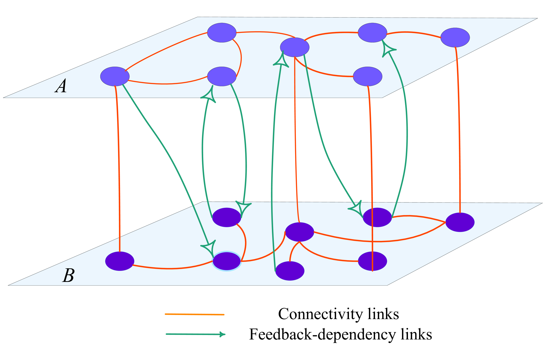
Figure 1: Demonstration of interacting networks with feedback dependency links. The feedback dependency links between network $A$ and network $B$ are random and directional. The nodes of $A$ and $B$ are randomly connected with connectivity links.

For two networks $A$ and $B$ of sizes $N_{A}$ and $N_{B}$, we assume that they are coupled by both dependency and connectivity links. For the case of dependency links, the two networks are partially coupled, which means dependency links between two fractions $q_{A}$ and $q_{B}$ of nodes in $A$ and $B$ networks satisfies the feedback condition (as shown in Fig. 1). For the other case, connectivity links connecting nodes within each network and between the networks, which can be presented by degree distributions $P^{A}_{(k_{A},k_{AB})}$, $P^{B}_{(k_{B},k_{BA})}$ respectively, where $P^{A}_{(k_{A},k_{AB})}$ and $P^{B}_{(k_{B},k_{BA})}$ denote the probability of an node in $A$ or ($B$) to have $k_{A}$ or ($k_{B}$) links to nodes in the same network and $k_{AB}$ or ($k_{BA}$) links toward other network. When nodes fail in a network, all connectivity links connected to these nodes fails, causing other nodes to disconnect from the network. Since dependency relations between networks, interdependent nodes in other network also remove along with their connectivity links. We assume that a functional node in network $A$ ($B$) must belong to the giant component of network $A$ ($B$). When this cascading process occur, it will stop if nodes that fail in one step do not cause additional failures and stabilizes with giant component.

When a fraction $1-p$ of $A$ nodes are initially removed, $g_{A}(\omega_{t},\varpi_{t})$ and $g_{B}(\omega_{t},\varpi_{t})$ are equal to the fraction of nodes in the giant components of networks $A$ and $B$ at step $t$, after removal of fractions $1-\omega_{t}$ and $1-\varpi_{t}$, respectively. Thus, the cascading dynamics can be described by

$$\begin{split}&\omega_{1}=p,\varpi_{1}=1,P_{1}^{A}=\omega_{1}g_{A}(\omega_{1},\varpi_{1}),\\ &\varpi_{2}=1-q_{B}(1-P_{1}^{A}),P_{2}^{B}=\varpi_{2}G_{B}(\omega_{1},\varpi_{2}),\\ &\omega_{2}=p[1-q_{A}(1-P_{2}^{B})],P_{2}^{A}=\omega_{2}g_{A}(\omega_{2},\varpi_{2}),\\ &\varpi_{3}=1-q_{B}(1-P_{2}^{A}),P_{3}^{B}=\varpi_{3}g_{B}(\omega_{2},\varpi_{3}),\\ &\omega_{3}=p[1-q_{A}(1-P_{3}^{B})],P_{3}^{A}=\omega_{3}g_{A}(\omega_{3},\varpi_{3}),\\ &\cdots\\ &\varpi_{t}=1-q_{B}(1-P_{t-1}^{A}),P_{t}^{B}=\varpi_{t}g_{B}(\omega_{t-1},\varpi_{t}),\\ &\omega_{t}=p[1-q_{A}(1-P_{t}^{B})],P_{t}^{A}=\omega_{t}g_{A}(\omega_{t},\varpi_{t}).\\ \end{split}$$ (1)

Where, $P_{t}^{A}$ ($P_{t}^{B}$) is the corresponding giant components of network $A$ ($B$).

For $\omega_{t}$, $\varpi_{t}$, $P_{t}^{B}$ and $P_{t}^{A}$, at $t\rightarrow\infty$, since eventually the clusters stop fragmenting. Thus, at steady state, the expression of system can be given by

$$\begin{split}&\varpi_{\infty}=1-q_{B}(1-P_{\infty}^{A}),P_{\infty}^{B}=\varpi_{\infty}g_{B}(\omega_{\infty},\varpi_{\infty}),\\ &\omega_{\infty}=p[1-q_{A}(1-P_{\infty}^{B})],P_{\infty}^{A}=\omega_{\infty}g_{A}(\omega_{\infty},\varpi_{\infty}).\end{split}$$ (2)

III Theory

In this paper, we consider the case where all degree distributions of the connectivity intra- and interlinks are Poissonian. Thus, the two-dimensional generating function are as follows Leicht2010 ; Hu2011

$$\begin{split}&G_{0}^{A}(x_{A},x_{B})=\sum_{k_{A},\bar{k}_{A}}P_{k_{A},\bar{k}_{A}}^{A}x_{A}^{k_{A}}x_{B}^{\bar{k}_{A}},\\ &G_{0}^{B}(x_{A},x_{B})=\sum_{k_{B},\bar{k}_{B}}P_{k_{B},\bar{k}_{B}}^{B}x_{A}^{\bar{k}_{B}}x_{B}^{k_{B}},\\ &G_{1}^{AB}(x_{A},x_{B})=\sum_{k_{A},\bar{k}_{A}}\frac{(\bar{k}_{A}+1)P_{k_{A},\bar{k}_{A}+1}^{A}}{\displaystyle\sum_{k^{{}^{\prime}}_{A},\bar{k}^{{}^{\prime}}_{A}}\bar{k}^{{}^{\prime}}_{A}P_{k^{{}^{\prime}}_{A},\bar{k}^{{}^{\prime}}_{A}}^{A}}x_{A}^{k_{A}}x_{B}^{\bar{k}_{A}}.\\ \end{split}$$ (3)

where, $(\bar{k}_{A}+1)P_{k_{A},\bar{k}_{A}+1}^{A}$ is the probability of following a randomly chosen $\bar{k}_{A}$ link connecting an $A$ node of degree $k_{A}$ to a $B$ node with excess $\bar{k}_{A}$ degree and $G_{1}^{AB}(x_{A},x_{B})$ is generating function of this distribution. Accordingly, the other three excess generating functions, $G_{1}^{AA},G_{1}^{BA},G_{1}^{BB}$, can be obtained Leicht2010 ; Hu2011

$$\begin{split}&G_{0}^{AA}(x_{A})=e^{k_{A}(x_{A}-1)},\\ &G_{0}^{AB}(x_{B})=e^{\bar{k}_{A}(x_{B}-1)},\\ &G_{0}^{BA}(x_{A})=e^{\bar{k}_{B}(x_{A}-1)},\\ &G_{0}^{BB}(x_{B})=e^{k_{B}(x_{B}-1)}.\end{split}$$ (4)

Thus, from Eqs.(3) and (4), the four excess function can be presented

$$\begin{split}&G_{1}^{AA}(x_{A},x_{B})=G_{1}^{AB}(x_{A},x_{B})=G_{0}^{A}(x_{A},x_{B})=G_{0}^{AA}(x_{A})G_{0}^{AB}(x_{B})=e^{k_{A}(x_{A}-1)}e^{\bar{k}_{A}(x_{B}-1)},\\ &G_{1}^{BB}(x_{A},x_{B})=G_{1}^{BA}(x_{A},x_{B})=G_{0}^{B}(x_{A},x_{B})=G_{0}^{BA}(x_{A})G_{0}^{BB}(x_{B})=e^{\bar{k}_{B}(x_{A}-1)}e^{k_{B}(x_{B}-1)}.\end{split}$$ (5)

After removal of $1-\omega$ and $1-\varpi$ fractions of network $A$ and $B$, from Eqs. (4) and (5), we have

$$\begin{split}&g_{A}(\omega,\varpi)=1-G_{0}^{A}[1-\omega(1-f_{A}),1-\varpi(1-f_{BA})],\\ &g_{B}(\omega,\varpi)=1-G_{0}^{B}[1-\omega(1-f_{AB}),1-\varpi(1-f_{B})].\end{split}$$ (6)

where,

$$\begin{split}&f_{A}=G_{1}^{AA}[1-\omega(1-f_{A}),1-\varpi(1-f_{BA})],\\ &f_{B}=G_{1}^{AB}[1-\omega(1-f_{AB}),1-\varpi(1-f_{B})],\\ &f_{AB}=G_{1}^{AB}[1-\omega(1-f_{A}),1-\varpi(1-f_{BA})],\\ &f_{BA}=G_{1}^{BA}[1-\omega(1-f_{AB}),1-\varpi(1-f_{B})].\end{split}$$ (7)

For cascading process, we compare our theoretical results obtained from Eqs. (1), (4), (5), (6) and (7) with results of numerical simulations as shown in Fig. 2. One can see that the simulation results show excellent agreement with the theory.

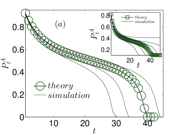
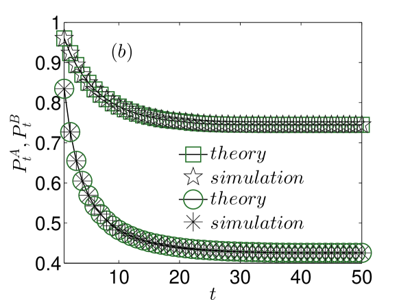
Figure 2: (a) Comparison between simulations and theory, the fraction $P^{A}_{t}$ of giant component of network $A$ as a function of stage $t$ with parameters $k_{A}=k_{B}=5$, $\bar{k}_{A}=\bar{k}_{B}=0.5$, $q_{B}=1$ and $N^{A}=N^{B}=10^{5}$. We choose parameters $q_{A}=0.8$, $p=0.928$ for main figure and $q_{A}=0.7$, $p=0.828$ for sub-figure. (b) The fraction $P^{A}_{t}$ ($\bigcirc$) , $P^{B}_{t}$ ($\Box$) of giant component of network $A$, $B$ as function of stage $t$ with the same parameters as in (a) but $q_{A}=0.7$, $p=0.843$. The simulation results are averaged over 50 realizations.

Submitting Eqs. (5), (6) and (7) into Eq. (2), at steady state, the corresponding $P_{\infty}^{A}$ and $P_{\infty}^{B}$ are expressed

$$P_{\infty}^{A} =p[1-q_{A}(1-P_{\infty}^{B})][1-e^{-(k_{A}P_{\infty}^{A}+\bar{k}_{A}P_{\infty}^{B})}],$$ (8)

$$P_{\infty}^{B} =1-q_{B}(1-P_{\infty}^{A})[1-e^{-(\bar{k}_{B}P_{\infty}^{A}+k_{B}P_{\infty}^{B})}].$$

We presents comparison the theoretical predictions and simulations for the giant components as a function of $q_{A}$ and $\bar{k}$ as shown in Fig. 3(a)-(b). One can see that the theory predictions from Eq. (8) agrees well with simulation results for different set of $q_{A}$ and $\bar{k}$ as shown in Fig. 3(a)-(b). Furthermore, we can clearly find that as coupling strength $q_{A}$ increases, the system undergoes second order transition to first order transition through hybrid order transition, which means the size of the giant component jumps at $p^{h,I}_{c}$ from a large value to a small value then continuously decreases at $p^{h,II}_{c}$ to zero. And, Fig. 3(a)-(b) also presents corresponding critical fraction $p_{c}$, including first and second order transition points $p^{I}_{c}$, $p^{II}_{c}$, two hybrid order transition points $p^{h,I}_{c}$, $p^{h,II}_{c}$. Additionally, the number of iterative failures ($NOI$) as a function of $\bar{k}$ and $p$ is shown in Fig. 3(c), one can observe that $NOI$ has a peak at jump points, $p^{I}_{c}$ and $p^{h,I}_{c}$. Thus, it provides a useful and precise method for identifying the transition points $p^{I}_{c}$ and $p^{h,I}_{c}$ by computing $NOI$ as a function of $p$.

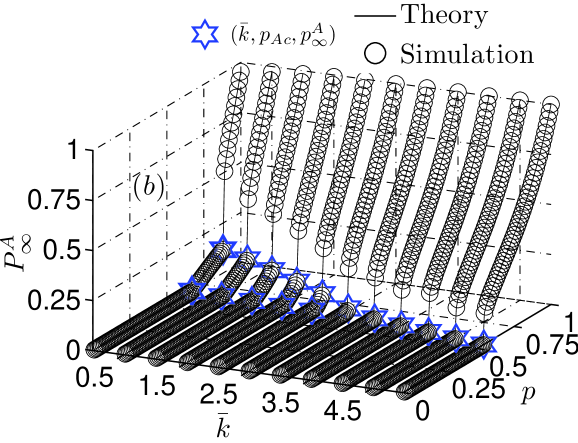
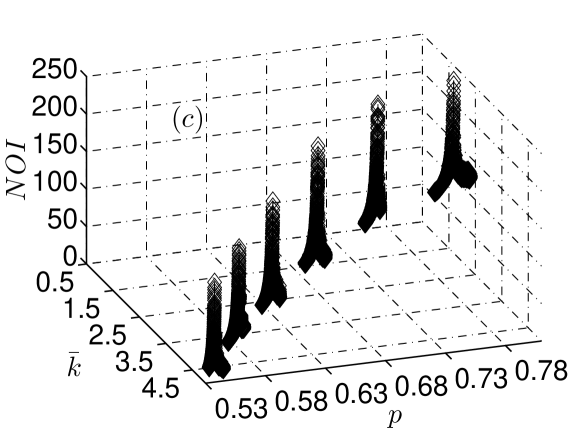
Figure 3: (a) Comparison between simulations and theoretical predictions, the fraction of giant component $p^{A}_{\infty}$ as a function of $p$ and $q_{A}$ with parameters $k_{A}=k_{B}=5$, $\bar{k}_{A}=\bar{k}_{B}=0.5$, $N_{A}=N_{B}=10^{5}$. (b) $p^{A}_{\infty}$ as a function of $p$ and $\bar{k}$ with the same parameters as in (a) but $k_{A}=k_{B}=5$. (c) $NOI$ as a function of $p$ and $\bar{k}$ with same parameter as in (b) from numerical analysis. The simulation results are averaged over 50 realizations.

In fact, Eqs. (8) can be solved graphically as shown in Fig. 4. For given parameters, Fig. 4 implies that the critical point $p^{I}_{c}$ and $p^{h,I}_{c}$ is the intersection of the two curves $P^{A}_{\infty}(P^{B}_{\infty})$ and $P^{B}_{\infty}(P^{A}_{\infty})$. Thus, the corresponding critical manifold can be found from the tangential condition

$$\frac{dP^{A}_{\infty}}{dP^{B}_{\infty}}\frac{dP^{B}_{\infty}}{dP^{A}_{\infty}}=1$$ (9)

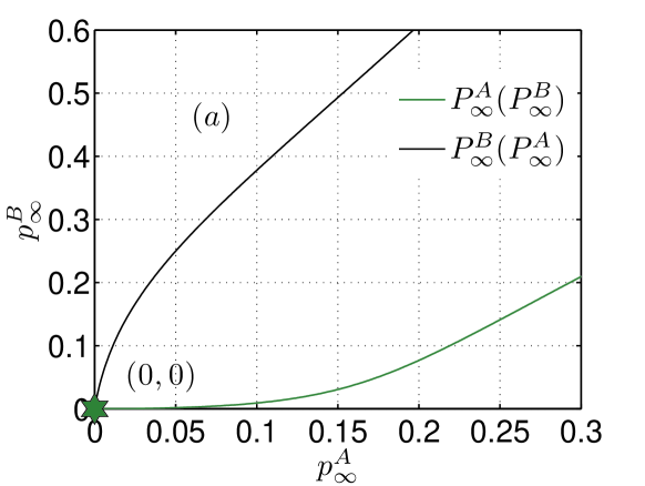
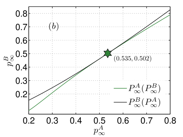
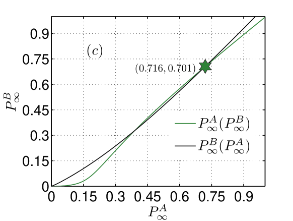
Figure 4: $P^{B}_{\infty}$ as a function of $P^{A}_{\infty}$ are shown from Eq. (8) with the different $p$, $p=0.6$ (a), $p=0.94$ (b), $p=0.96$ (c). One can see that as $p<0.94$, only a trivial solution $P^{A}_{\infty}=P^{B}_{\infty}=0$ exists from (a). As $p=0.94$, the non-zero giant component of both networks appears at stable state from (b). As $p=0.96>0.94$, the largest solution of two curves is chosen, since the size of giant component gradually decreases at cascading process.

From above analysis, the coupling strength $q_{A}$ as a function of $p$ is studied from Eqs. (8) and (9), as shown in Fig. 5(a)-(c). We can observe that as $q\in[0,q^{S,H}_{Ac}]$, the system only occurs second order transition at $p^{II}_{c}$ from Fig. 5(a)-(c), where coupling strength $q^{S,H}_{Ac}$ is a boundary point of between second order region and hybrid order region. As $q\in(q^{S,H}_{Ac},q^{H,F}_{Ac}]$, the system undergoes hybrid order transition and have two critical points $p^{h,II}_{c}$ and $p^{h,I}_{c}$, where coupling strength $q^{H,F}_{Ac}$ is a boundary point of between hybrid order region and first order region. Similarly, as $q>q^{H,F}_{Ac}$, the system only behaves first order transition and $p^{I}_{c}$ appears. Furthermore, we can observe that when system occurs second order transition behaviors, $p^{II}_{c}$ has a little change as $\bar{k}$ increases from Fig. 5(d), which implies that $\bar{k}$ has a little influence to robustness of system for weak coupling. However, when system only undergoes first order transition behaviors for strong coupling, $p^{I}_{c}$ decreases and system become more robust as $\bar{k}$ increases. Especially, for coupling strength $q_{A}$ corresponding hybrid order transition, $p^{h,II}_{c}$ keep constant, $p^{h,I}_{c}$ decreases and eventually coincidence, which suggests that hybrid order region disappears. However, as $k$ increases, one can see that all the critical points $p_{c}$ increases as $k$ increases from Fig. 5(d), which means the system become robust as average degree of inter-network increases. Fig. 6(a) and (b) describe that the phase transition region changes as $\bar{k}$ and $k$ increase. We can see that first order region gradually become larger due to $q^{H,F}_{Ac}$ increases as $\bar{k}$ increases from Fig. 6(a). Meanwhile, since the difference between $q^{H,F}_{Ac}$ and $q^{S,H}_{Ac}$ become smaller, the hybrid order region become smaller and eventually disappear as $\bar{k}$ increases. At this time, the system only occur first order transition. Additionally, when $k$ increases, first order region becomes smaller and second-order region becomes larger but hybrid order region almost keep constant.

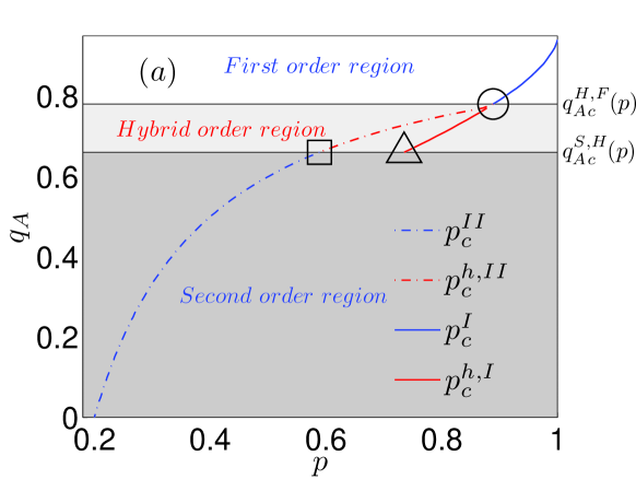
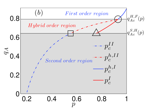
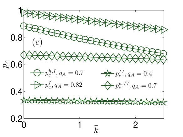
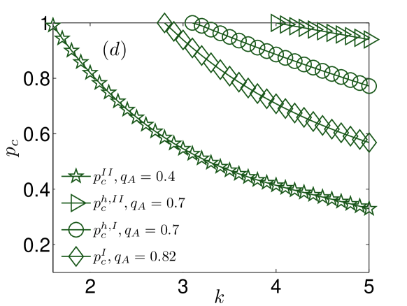
Figure 5: The coupling strength $q_{A}$ as a function of $p$ for different parameter $\bar{k}$ with parameters $k_{A}=k_{B}=k=5$, $\bar{k}_{A}=\bar{k}_{B}=\bar{k}$ and $q_{B}=1$. (a) $\bar{k}=1$. (b) $\bar{k}=0.5$. (c) $p_{c}$ as a function of $\bar{k}$ for different $q_{A}$ with parameters $k_{A}=k_{B}=k=5$ and $q_{B}=1$. (d) $p_{c}$ as a function of $k$ for different $q_{A}$ with parameters $\bar{k}_{A}=\bar{k}_{B}=\bar{k}=0.5$ and $q_{B}=1$.

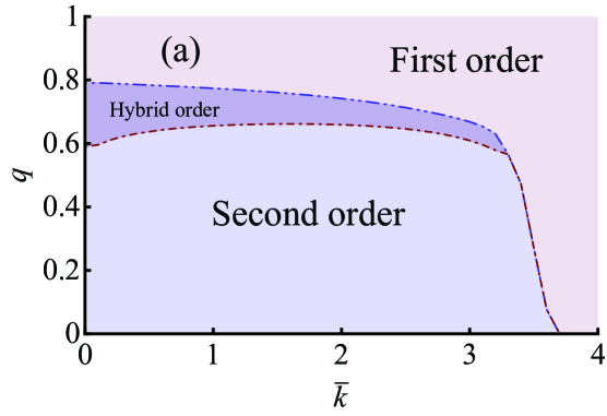
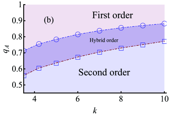
Figure 6: The coupling strength $q_{A}$ as a function of $\bar{k}$ (a) and $k$ (b) at the critical faction $p_{c}$. (a) the parameters are $k_{A}=k_{B}=k=5$, $\bar{k}_{A}=\bar{k}_{B}=\bar{k}$ and $q_{B}=1$. (b) The parameters are the similar with (a) but $\bar{k}=0.5$. The blue and red dash line denote $q^{H,F}_{Ac}$ and $q^{S,H}_{Ac}$ respectively.

Furthermore, we compare our model with model under non-feedback condition for two interacting networks. For the same parameters, by comparing Fig. 7(a) with Fig. 5(b), one can find that when dependency links satisfy feedback condition, $p_{c}$ is more bigger than that under non-feedback condition. Thus, for two coupling links, feedback condition between two networks make the system extremely vulnerable, which means that the system is difficult to defend for feedback condition. And, for feedback condition, $q^{H,F}_{Ac}$ and $q^{S,H}_{Ac}$ are smaller than that under non-feedback condition, which means the system have bigger first order region under randomly attacking as shown in Fig. 7(b).

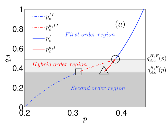
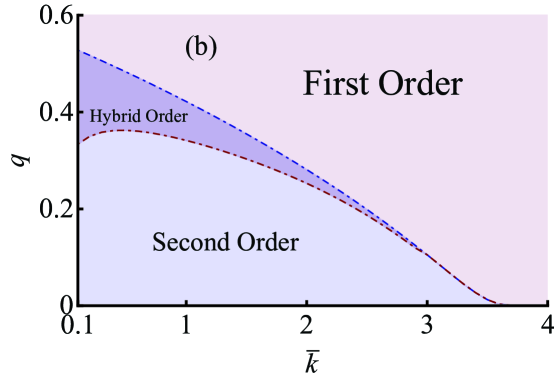
Figure 7: (a) The coupling strength $q_{A}$ as a function of $\bar{k}$ at the critical faction $p_{c}$ under non-feedback condition for the same parameters with Fig. 5(b). (b) The coupling strength $q_{A}$ as a function of $p$ for different parameter $\bar{k}$ for the same parameters with Fig. 6(a).

IV conclusion

In summary, we have introduced a framework for two interacting network with feedback dependency links. Our theory is in excellent agreement with the numerical simulations on coupled networks with Poissonian distribution, which also can be applied to any degree distribution networks. We find that for weak coupling strength, $p^{II}_{c}$ has a little change and robustness of system is not altered significantly as $\bar{k}$ increases. But for strong coupling strength, $p^{I}_{c}$ decreases and the system become more robust as $\bar{k}$ increases. However, for all the coupling strength, the system become robust as $k$ increases. Moreover, as $\bar{k}$ increases, $q^{S,H}_{Ac}$ and $q^{H,F}_{Ac}$ gradually become small and eventually coincidence, which means that hybrid order region disappears, and meanwhile the system only occurs first and second phase transitions. Additionally, by comparing non-feedback dependency condition between interacting networks, we find that the system is extremely vulnerable and difficult to defend for cascading failures.

V acknowledgments

References

- (1) D. J. Watts and S. H. Strogatz, Nature 393, 440 (1998).
- (2) A. -L. Barabási and R. Albert, Science 286, 509(1999).
- (3) R. Albert and A. -L. Barabasi, Rev. Mod. Phys. 74, 47(2002).
- (4) R. Cohen, K. Erez, D. Ben-Avraham, and S. Havlin, Phys. Rev. Lett. 85, 4626 (2000); Phys. Rev. Lett. 86, 3682 (2001).
- (5) D. S. Callaway, M. E. J. Newman, S. H. Strogatz, and D. J. Watts, Phys. Rev. Lett. 85, 5468 (2000).
- (6) S. N. Dorogovtsev and J. F. F. Mendes, Evolution of Networks: From Biological Nets to the Internet and WWW(Physics) (Oxford Univ. Press, New York, 2003).
- (7) R. P. Satorras and A.Vespignani, Evolution and Structure of the Internet: A Statistical Physics Approach (Cam-bridge Univ. Press, England, 2006).
- (8) A. Bashan et al, Nature Comm. 3, 702 (2012).
- (9) C. Song, S. Havlin, and H. A. Makse, Nature 433, 392 (2005).
- (10) R. Cohen and S. Havlin, Complex Networks: Structure, Robustness and Function (Cambridge Univ. Press, England, 2010).
- (11) G. Caldarelli and A. Vespignani, Large scale Structure and Dynamics of Complex Webs (World Scientific, Singapore, 2007).
- (12) M. E. J. Newman, Networks: An Introduction (Oxford Univ. Press, New York, 2010).
- (13) Y. Hu, Y. Wang, D. Li, S. Havlin, Z. Di, Phys. Rev. Lett. 106, 108701 (2011).
- (14) R. Liu, W. Wang, Y. Lai, B. Wang, Phys. Rev. E. 85, 026110 (2012).
- (15) Z. Rong, H. Yang, W. Wang, Phys. Rev. E. 82, 047101 (2010).
- (16) H. Yang, Z. Wu, B. Wang, Phys. Rev. E. 81, 065101 (2010).
- (17) M. Dai, X. Li, D. Li, L. Xi, Chaos 23, 033106 (2013).
- (18) D. Li, K. Kosmidis, A. Bunde, S. Havlin, Nature physics 7, 481 (2011).
- (19) Q. Li, L. A. Braunstein, S. Havlin, and H. E. Stanley, Phys. Rev. E 84, 06601 (2011).
- (20) Y. Li, E. Csóka, H. Zhou, and M. Pósfai, Phys. Rev. Lett. 109, 205703 (2012).
- (21) S. Havlin et al., arXiv:1012.0206v1.
- (22) S. V. Buldyrev et al., Nature 464, 1025 (2010).
- (23) E. A. Leicht, R. M. D́Souza, e-print arXiv:0907.0894.
- (24) J. Shao, Buldyrev, S. V., Braunstein, L. A., Havlin, S. and H. E. Stanley, Phys. Rev. E 80, 036105 (2009).
- (25) R. Parshani, S.V. Buldyrev, S. Havlin, PNAS 108, 1007 (2011).
- (26) Y. Hu, B. Ksherim, R. Cohen, S. Havlin, Phys. Rev. E 84, 066116 (2011).
- (27) J. Gao, S. V. Buldyrev, S. Havlin, and H. E. Stanley, Nature physics 8, 40 (2012).
- (28) A. Bashan, R. Parshani, S. Havlin, Phys. Rev. E 83, 051127 (2011).
- (29) R. Parshani, S. V. Buldyrev, and S. Havlin, Phys. Rev. Lett. 105, 048701 (2010).
- (30) G. Dong, J. Gao, L. Tian, R. Duo, and Y. He, Phys. Rev. E 85, 016112 (2012).
- (31) J. Gao, S. V. Buldyrev, S. Havlin, and H. E. Stanley, Phys. Rev. Lett. 107, 195701 (2011).
- (32) X. Q. Huang et al., Phys. Rev. E 83, 065101(R) (2011).
- (33) W. Li, S. V. Buldyrev, H. E. Stanley, S. Havlin, Phys. Rev. Lett. 108, 228702 (2012).
- (34) G. Dong, J. Gao, R. Du, L. Tian, H.E. Stanley, S. Havlin, Phys. Rev. E 87, 052804 (2013).
- (35) D. Zhou, J. Gao, H.E. Stanley, S. Havlin, Phys. Rev. E 87, 052812 (2013).
- (36) G. Dong, L. Tian, D. Zhou, R. Du, J. Xiao, and H. E. Stanley, EPL 102, 68004 (2013).
- (37) H. Wang, Q. Li, G. D́Agostino, S. Havlin, H.E. Stanley, P. Van Mieghem, Phys. Rev. E 88, 022801 (2013).