Rate of Convergence of Phase Field Equations in Strongly Heterogeneous Media towards their Homogenized Limit

Abstract

We study phase field equations based on the diffuse-interface approximation of general homogeneous free energy densities showing different local minima of possible equilibrium configurations in perforated/porous domains. The study of such free energies in homogeneous environments found a broad interest over the last decades and hence is now widely accepted and applied in both science and engineering. Here, we focus on strongly heterogeneous materials with perforations such as porous media. To the best of our knowledge, we present a general formal derivation of upscaled phase field equations for arbitrary free energy densities and give a rigorous justification by error estimates for a broad class of polynomial free energies. The error between the effective macroscopic solution of the new upscaled formulation and the solution of the microscopic phase field problem is of order $\epsilon^{1/2}$ for a material given characteristic heterogeneity $\epsilon$. Our new, effective, and reliable macroscopic porous media formulation of general phase field equations opens new modelling directions and computational perspectives for interfacial transport in strongly heterogeneous environments.

Keywords: Free energies, Cahn-Hilliard/Ginzburg-Landau equations, multiscale modeling, homogenization, porous media, wetting, phase transformations

1 Introduction

We consider the well-accepted diffuse-interface formulation [11, 47] for studying the evolution of interfaces between different phases. Its broad applicability together with increasing computational power enables its use to new and increasingly complex scientific and engineering settings such as the computation of transport equations in porous media [36] which represents a numerically very demanding, high-dimensional multiscale problem [24]. The purpose of the present work is to rigorously and systematically provide an analytically and computationally reliable effective macroscopic description of how multiple phases invade strongly heterogeneous media such as porous materials for instance.

We consider the abstract energy density

$$\begin{split}e(\phi):=\frac{1}{\lambda}F(\phi)+\frac{\lambda}{2}\left|\nabla\phi\right|^{2}\,,\end{split}$$ (1.1)

where $\phi:=\frac{c_{\beta}}{c_{\alpha}+c_{\beta}}$ is a reduced order parameter representing the fraction of a single species $\beta$ in a binary solution containing species $\alpha$ and $\beta$ with densities $c_{\alpha}$ and $c_{\beta}$, respectively. The gradient term $\lambda^{2}\left|\nabla\phi\right|^{2}$ penalizes the interfacial area between these phases, and $F$ is defined as the general (Helmholtz) free energy density

$$\begin{split}F(\phi)&:=U-TS\,,\end{split}$$ (1.2)

where $U$ stands for the internal energy, $T$ the temperature, and $S$ the entropy. Important examples for applications include the regular solution theory (also known as the Flory-Huggins energy density [16])

$$\begin{split}F(\phi)&:=R(\phi)-TS_{I}(\phi)\,,\end{split}$$ (1.3)

where $S_{I}(\phi):=-k_{B}\left[\phi{\rm ln}\,\phi-(1-\phi){\rm ln}\,(1-\phi)\right]$ is the entropy of mixing for ideal solutions and the regular solution term $R(\phi):=z\omega\phi(1-\phi)$ accounts for the interaction energy between different species. The variable $z$ is the coordination number defining the number of bonds of $\beta$ with neighbouring species. $\omega:=\epsilon_{\alpha\alpha}+\epsilon_{\beta\beta}-2\epsilon_{\alpha\beta}$ is the interaction energy parameter accounting for the minima $\epsilon_{\alpha\alpha}$, $\epsilon_{\beta\beta}$, and $\epsilon_{\alpha\beta}$ of interaction potentials which define attractive and repulsive forces between the species $\alpha$ and $\beta$.

The regular solution theory is of great importance in many different contexts such as ionic melts [21], water sorption in porous solids [6, 7], and micellization in binary surfactant mixtures [23]. Also wetting phenomena, of great interest in technological applications, especially motivated by recent developments in micro-fluidics, are often studied using classical sharp-interface approximations, e.g. [37, 38, 39], but also enjoy a wide-spread use of phase-field modeling [34, 49, 48, 44] also including the presence of an electric field (electrowetting, e.g. [13, 29]). Furthermore, transport in an electrochemical system consisting of an electrolyte and an electrode [19], or immiscible flows [25] under a polynomial free energy in the form of the classical double-well potential, i.e., $W(\phi):=\frac{1}{4}(1-\phi^{2})^{2}$ are relevant applications. Our formal derivation of upscaled phase equations is valid for general free energies but the derivation of error estimates is based on free energies to the following

Polynomial Class (PC): Admissible free energy densities $F$ in (1.1) are polynomials of order $2r-1$, i.e.,

$$\begin{split}f(u)=\sum_{i=1}^{2r-1}a_{i}u^{i}\,,\quad r\in\mathbb{N}\,,\quad r\geq 2\,,\end{split}$$ (1.4)

with $f(u)=F^{\prime}(u)$ vanishing at $u=0$, that is,

$$\begin{split}F(u)=\sum_{i=2}^{2r}b_{i}u^{i}\,,\quad ib_{i}=a_{i-1}\,,\quad 2\leq i\leq 2r\,,\end{split}$$ (1.5)

where the leading coefficient of both $F$ and $f$ is positive, i.e., $a_{2r-1}=2rb_{2r}>0$.

Temam [46] established well-posedness of the Cahn-Hilliard equation for free energies of class (PC). Phase-field energy functionals are also of interest in image processing such as inpainting, see e.g. [10]. We note that for computational stability one often replaces the regular solution energy density (1.3) by the polynomial double-well potential $W(\phi)$.

In difference to the approach in [43], we provide here an upscaling strategy that is valid for general homogeneous free energy densities due to the application of a functional Taylor expansion around the effective upscaled solution and hence provides a convenient methodology for the homogenization of nonlinear problems. Moreover, we present here, to the best of our knowledge for the first time, error estimates between the solution of the microscopic phase field equations solved in a periodic porous medium and the solution of the correspondingly homogenized/upscaled equations by Theorem 3.5. In the remaining part of this section, we introduce the basic setting where we want to study the dynamics of interfaces.

(a) Homogeneous domains $\Omega$. In the Ginzburg-Landau/Cahn-Hilliard formulation, the total energy is defined by $E(\phi):=\int_{\Omega}e(\phi)\,d{\bf x}$ with density (1.1) on a bounded domain $\Omega\subset\mathbb{R}^{d}$ with smooth boundary $\partial\Omega$ and $1\leq d\leq 3$ denotes the spatial dimension. In general, the local minima of $F$ correspond to the equilibrium limiting values of $\phi$ representing different phases separated by a diffuse interface whose spatial extension is governed by the gradient term. It is well accepted that thermodynamic equilibrium can be achieved by minimizing the energy $E$, here supplemented by a possible boundary contribution $\int_{\partial\Omega}g({\bf x})\,d{\bf x}$ for $g({\bf x})\in H^{3/2}(\partial\Omega)$ where $do$ denotes the surface measure. A widely used minimization over time forms the $H^{-1}$-gradient flow with respect to $E(\phi)$, i.e.,

$$\begin{split}\textrm{(Homogeneous case)}\,\,\,\begin{cases}\frac{\partial}{\partial t}\phi={\rm div}\left(\hat{\rm M}\nabla\left(\frac{1}{\lambda}f(\phi)-\lambda\Delta\phi\right)\right)&\quad\textrm{in }\Omega_{T}\,,\\ \nabla_{n}\phi:={\bf n}\cdot\nabla\phi=g({\bf x})&\quad\textrm{on }\partial\Omega_{T}\,,\\ \nabla_{n}\Delta\phi=0&\quad\textrm{on }\partial\Omega_{T}\,,\end{cases}\end{split}$$ (1.6)

where $\Omega_{T}:=\Omega\times]0,T[$, $\partial\Omega_{T}:=\partial\Omega\times]0,T[$, $\phi$ satisfies the initial condition $\phi({\bf x},0)=\psi({\bf x})$, and $\hat{\rm M}=\left\{{\rm m}_{ij}\right\}_{1\leq i,j\leq d}$ denotes a mobility tensor with real and bounded elements ${\rm m}_{ij}>0$. The gradient flow (1.6) is weighted by the mobility tensor $\hat{\rm M}$, and is referred to as the Cahn-Hilliard equation. This equation is a model prototype for interfacial dynamics [e.g. [15]] and phase transformation [e.g. [11]] under homogeneous Neumann boundary conditions, i.e., $g=0$, and free energy densities $F$. The mean free energy density (1.1) can be derived by a thermodynamic limit from lattice gas models of filled and empty sites for instance. We note that the double-well potential $W$ is related to the Lennard-Jones potential in the sense of the LMP (Lebowitz, Mazel and Presutti) theory [35] but cannot be exactly reduced to the atomistic Lennard-Jones potential. Finally, we note that we applied a scaling with respect to $\lambda$ which allows to identify the Hele-Shaw/Mullins-Sekerka problem in the limit $\lambda\to 0$ which is rigorously derived in [2] and discussed below.

It is well-known, that formally, the integrated energy density (1.1) dissipates along solutions of the gradient flow (1.6), that means, $E(\phi(\cdot,t))\leq E(\phi(\cdot,0))=:E_{0}$, see (2.19) and (2.20). This follows immediately after differentiating (1.1) with respect to time and using (1.6) for $g=0$. Moreover, we emphasize the interesting connection of the Cahn-Hilliard/phase field equation to the complicated free boundary value problem known as the Mullins-Sekerka problem [27] or the two-phase Hele-Shaw problem [20]. Inspired by the formal derivation by Pego [33], it was rigorously verified later on by [2, 45] that the chemical potential $\mu(\phi):=-\lambda\Delta\phi+\frac{1}{\lambda}f(\phi)\,,$ satisfies in the limit $\lambda\to 0$ for $t\in[0,T]$ the following

$$\begin{split}\textrm{Hele-Shaw/Mullins-Sekerka problem:}\qquad\begin{cases}\quad\Delta\mu=0&\quad\textrm{in }\Omega\setminus\Gamma_{t}\,,\\ \quad{\bf n}\cdot\nabla\mu=0&\quad\textrm{on }\partial\Omega\,,\\ \quad\mu=\sigma\kappa&\quad\textrm{on }\Gamma_{t}\,,\\ \quad v=\frac{1}{2}\left[{\bf n}\cdot\nabla\mu\right]_{\Gamma_{t}}&\quad\textrm{on }\Gamma_{t}\,,\\ \quad\Gamma_{0}=\Gamma_{00}&\quad\textrm{if }t=0\,,,\end{cases}\end{split}$$ (1.7)

where $\sigma=\int_{-1}^{1}\left(\frac{1}{2}\int_{0}^{s}f(r)\,dr\right)^{1/2}\,ds$ is the interfacial tension, $\kappa$ the mean curvature, $v$ the normal velocity of the interface $\Gamma_{t}$, ${\bf n}$ the unit outward normal to either $\partial\Omega$ or $\Gamma_{t}$, and $\left[{\bf n}\cdot\nabla\mu\right]_{\Gamma_{t}}:={\bf n}\cdot\nabla\mu^{+}-{\bf n}\cdot\nabla\mu^{-}$ where $\mu^{+}:=\mu\,\bigr{|}_{\Omega^{+}_{t}}$ and $\mu^{-}:=\mu\,\bigl{|}_{\Omega^{-}_{t}}$ and $\Omega^{+}_{t}$ and $\Omega^{-}_{t}$ denote the exterior and interior of $\Gamma_{t}$ in $\Omega$. Herewith, we also have $\phi\to\pm 1$ in $\Omega^{\pm}_{t}$ for all $t\in[0,T]$ as $\lambda\to 0$.

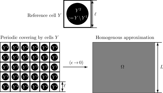
Figure 1: Left: Strongly heterogeneous/perforated material as a periodic covering of reference cells $Y:=[0,\ell]^{d}$. Top, middle: Definition of the reference cell $Y=Y^{1}\cup Y^{2}$ with $\ell=1$. Right: The “homogenization limit” $\epsilon:=\frac{\ell}{L}\to 0$ scales the perforated domain such that perforations become invisible on the macroscale.

(b) Heterogeneous/perforated domains $\Omega^{\epsilon}$. Here we study the energy density (1.1) with respect to a perforated domain $\Omega^{\epsilon}\subset\mathbb{R}^{d}$ instead of a homogeneous $\Omega\subset\mathbb{R}^{d}$. The dimensionless variable $\epsilon>0$ defines the heterogeneity $\epsilon=\frac{\ell}{L}$ where $\ell$ represents the characteristic pore size and $L$ is the characteristic length of the porous medium, see Figure 1. Hence, the porous medium is characterized by a reference cell $Y:=[0,\ell_{1}]\times[0,\ell_{2}]\times\dots\times[0,\ell_{d}]$ which represents a single, characteristic pore. For simplicity, we set $\ell_{1}=\ell_{2}=\dots=\ell_{d}=1$. A well-accepted approximation is then the periodic covering of the macroscopic porous medium by such a single reference cell $\epsilon Y$, see Figure 1. The pore and the solid phase of the medium are denoted by $\Omega^{\epsilon}$ and $B^{\epsilon}$, respectively. These sets are defined by,

$$\begin{split}\Omega^{\epsilon}&:=\bigcup_{{\bf z}\in\mathbb{Z}^{d}}\epsilon\left(Y^{1}+{\bf z}\right)\cap\Omega\,,\qquad B^{\epsilon}:=\bigcup_{{\bf z}\in\mathbb{Z}^{d}}\epsilon\left(Y^{2}+{\bf z}\right)\cap\Omega=\Omega\setminus\Omega^{\epsilon}\,,\end{split}$$ (1.8)

where the subsets $Y^{1},\,Y^{2}\subset Y$ are such that $\Omega^{\epsilon}$ is a connected set. More precisely, $Y^{1}$ stands for the pore phase (e.g. liquid or gas phase in wetting problems), see Figure 1.

These definitions allow us to reformulate (1.6) by the following microscopic porous media problem

$$\begin{split}\textrm{(Micro porous case)}\,\,\,\begin{cases}\quad\partial_{t}\phi_{\epsilon}={\rm div}\left(\hat{\rm M}\nabla\left(-\lambda\Delta\phi_{\epsilon}+\frac{1}{\lambda}f(\phi_{\epsilon})\right)\right)&\quad\textrm{in }\Omega^{\epsilon}_{T}\,,\\ \quad\nabla_{n}\phi_{\epsilon}:={\bf n}\cdot\nabla\phi_{\epsilon}=0&\quad\textrm{on }\partial\Omega^{\epsilon}_{T}\,,\\ \quad\nabla_{n}\Delta\phi_{\epsilon}=0&\quad\textrm{on }\partial\Omega^{\epsilon}_{T}\,,\\ \quad\phi_{\epsilon}({\bf x},0)=\psi({\bf x})&\quad\textrm{on }\Omega^{\epsilon}\,.\end{cases}\end{split}$$ (1.9)

In the next section, we motivate our main goal of deriving a homogenized, upscaled problem by passing to the limit $\epsilon\to 0$ in (1.9).

In Section 2, we give relevant reformulations of phase field equations and introduce basic notations and mathematical assumptions. The main theorems, which state the new effective macroscopic phase field formulation (Theorem 3.3) and the associated error (Theorem 3.5) between the solution of the upscaled problem which reliably accounts for the microstructure by homogenization and the solution of the microscopic problem fully resolving the pores in Section 3. The justification of these results then follow in Sections 4 and 5. Conclusions and suggestions for further work are given in Section 6.

2 Mathematical preliminaries and notation

We present two equivalent formulations of the Cahn-Hilliard equation. The first helps to achieve solvability for Lipschitz inhomogeneities and the second, referred to as “splitting formulation”, decouples the Cahn-Hilliard equation into two second order problems for a feasible upscaling by the multiple-scale method.

(i) Zero mass formulation (for well-posedness) [30] proves well-posedness of a differently scaled Cahn-Hilliard problem (1.6) rewritten for $\Omega_{T}:=\Omega\times]0,T[$ and $\partial\Omega_{T}:=\partial\Omega\times]0,T[$ in the following zero mass formulation

$$\begin{split}\textrm{\bf(Zero mass)}\quad\begin{cases}\quad\partial_{t}v={\rm div}\left(\hat{\rm M}/\lambda\nabla\left(bv+h(v)-\lambda\Delta v\right)\right)&\quad\textrm{in }\Omega_{T}\,,\\ \quad\nabla_{n}v={\bf n}\cdot\nabla\Delta v=0&\quad\textrm{on }\partial\Omega_{T}\,,\\ \quad v({\bf x},0)=v_{0}({\bf x})=\psi({\bf x})-\overline{\phi}\,&\quad\textrm{in }\Omega,\end{cases}\end{split}$$ (2.10)

where $v({\bf x},t):=\phi({\bf x},t)-\overline{\phi}$, $b:=f^{\prime}(\phi)$, $h(v):=f(\overline{\phi}+v)-bv$, and by mass conservation of (1.6) we define $\frac{1}{\left|\Omega\right|}\int_{\Omega}\phi\,d{\bf x}:=\frac{1}{\left|\Omega\right|}\int_{\Omega}\psi\,d{\bf x}=:\overline{\phi}\,.$ These definitions imply $bv+h(v)=f(\overline{\phi}+v)$. We introduce the space

$$\begin{split}H^{2}_{E}(\Omega)=\left\{\phi\in H^{2}(\Omega)\,\Bigr{|}\,\nabla_{n}\phi=0\textrm{ and }\overline{\phi}=0\right\}\,.\end{split}$$ (2.11)

[30] verifies local existence and uniqueness of solutions $v\in H^{2}_{E}(\Omega)$ of problem (2.10) for $f\in C^{2}_{Lip}(\mathbb{R})$ with $\left|f(s)\right|\to\infty$ as $s\to\pm\infty$ and $v({\bf x},0)\in H^{2}_{E}(\Omega)$. Moreover, in [30] one also finds necessary conditions on $h$ leading to global existence.

(ii) Splitting (for homogenization) By identifying $\phi=(-\Delta)^{-1}w$ in the $H^{2}_{E}(\Omega)$-sense, we are able to introduce the following problem

$$\begin{split}\textrm{\bf(Splitting)}\quad\begin{cases}\quad\partial_{t}(-\Delta)^{-1}w-\lambda{\rm div}\left(\hat{\rm M}\nabla w\right)={\rm div}\left(\frac{\hat{\rm M}}{\lambda}\nabla f(\phi)\right)&\textrm{in }\Omega_{T}\,,\\ \quad\nabla_{n}w=-\nabla_{n}\Delta\phi=0&\textrm{on }\partial\Omega_{T}\,,\\ \quad-\Delta\phi=w&\textrm{in }\Omega_{T}\,,\\ \quad\nabla_{n}\phi=g({\bf x})&\textrm{on }\partial\Omega_{T}\,,\\ \quad\phi({\bf x},0)=\psi({\bf x})&\textrm{in }\Omega\,,\end{cases}\end{split}$$ (2.12)

which is equivalent to (1.6) in the $H^{2}_{E}$-sense and hence, when $g=0$, is well-posed too, [30]. The advantage of (2.12) is that it allows to base our upscaling approach on well-known results from elliptic/parabolic homogenization theory [9, 22, 32, 50]. Finally, we remark that the splitting (2.12) slightly differs from the strategy applied for computational purposes in [4], for instance.

For the derivation of a priori estimates (partially based on [2]), the following general characterization of the homogeneous free energy $f=F^{\prime}$ proves to be very useful.

Assumption A:

• $F\in C^{4}(\mathbb{R})$ satisfies $F(\pm 1)=0$ and $F>0$ elsewhere.

• $F^{\prime}(u)$ satisfies for some finite $\alpha>2$ and positive constants $k_{i}>0$, $i=0,\dots,3$,

  $$\begin{split}k_{0}\left|u\right|^{\alpha-2}-k_{1}\leq F^{\prime}(u)\leq k_{2}\left|u\right|^{\alpha-2}+k_{3}\,.\end{split}$$ (2.13)

• There exist constants $0<a_{1}\leq 1$, $a_{2}>0$, $a_{3}>0$ and $a_{4}>0$ such that

  $$\begin{split}\left(F(a)-F(b),a-b\right)&\geq a_{1}\left(F^{\prime}(a)(a-b),a-b\right)-a_{2}\left|a-b\right|^{2+a_{3}}\qquad\forall\left|a\right|\leq 2a_{4}\,,\\ aF^{\prime\prime}(a)&\geq 0\qquad\forall\left|a\right|\geq a_{4}\,.\end{split}$$ (2.14)

It is straightforward to check that the classical double-well potential $F(x)=(x^{2}-1)^{2}/4$ satisfies Assumptions A. In order to obtain more regular solutions, we make the following assumptions on the initial condition [2].

Assumption B: There exist uniform constants $m_{0},\,\sigma_{j}>0$, $j=1,2,3$ such that

• $-1<m_{0}:=\frac{1}{\left|\Omega\right|}\int_{\Omega}\psi({\bf x})\,d{\bf x}<1\,,$

• ${\cal E}_{\lambda}(\psi):=\frac{\lambda}{2}\left\|\nabla\psi\right\|^{2}+\frac{1}{\lambda}\left\|F(\psi)\right\|_{L^{1}}\leq C\lambda^{-2\sigma_{1}}\,,$

• $\left\|\omega^{\lambda}\right\|_{H^{l}}:=\left\|-\lambda\Delta\psi+\frac{1}{\lambda}F(\psi)\right\|_{H^{l}}\leq C\lambda^{-\sigma_{2+l}}\,,\quad l=0,1\,.$

Next, we derive some a priori estimates which provide us the necessary bounds for our main result (Theorem 3.3) quantifying the error between the solution of the exact microscopic problem and the solution of the upscaled macroscopic equations (Theorem 3.5).

Lemma 2.1.

(A priori estimates) We assume that $f$ and $\psi$ satisfy the Assumptions A and B. Moreover, we suppose that the Mullins-Sekerka problem (1.7) has a global in time classical solution. Then, the solution $\phi$ of the Cahn-Hilliard equation (1.6) satisfies

$$\begin{split}\left\|\phi\right\|_{L^{\infty}(\Omega_{T})}\leq C\,,\end{split}$$ (2.15)

for all $\lambda\in]0,\kappa[$ and a family of smooth initial data $\left\{\psi^{\lambda}\right\}_{0<\lambda\leq 1}$ where $\kappa$ and $C$ are constants.

Moreover, for a solution $\phi$ of (1.6) the following estimate holds

$$\begin{split}\int_{0}^{\infty}\left\|\nabla\Delta\phi\right\|^{2}\,dt\leq C(\lambda)\,,\end{split}$$ (2.16)

for a constant $C>0$. If for a constant $\kappa>0$ the additional inequality

$$\begin{split}\lim_{s\to 0^{+}}\left\|\nabla\partial_{t}\phi(s)\right\|\leq C\lambda^{-\kappa}\,,\end{split}$$ (2.17)

holds, then the solution of (1.6) also satisfies for a large enough constant $C>0$

$$\begin{split}\left\|\Delta^{2}\phi\right\|_{L^{\infty}([0,\infty[;L^{2}(\Omega))}\leq C\lambda^{-C}\,.\end{split}$$ (2.18)

Remark 2.2.

(Hele-Shaw) Existence and uniqueness of classical soltuions for the so-called single phase Hele-Shaw problem in bounded domains in $\mathbb{R}^{d}$ has been proved in [14]. Another proof for the existence of a global in time classical solution for the multi-dimensional Hele-Shaw problem can be found in [26].

Proof.

i) Estimate (2.15): A proof based on asymptotic analysis and the construction of approximate solutions can be found in [2].
ii) Estimate (2.16): This inequality is based on (2.15) and the following basic energy estimate for the Cahn-Hilliard equation, i.e.,

$$\begin{split}\frac{dE(\phi)}{dt}=\left(\nabla_{\phi}^{L^{2}}E(\phi),\frac{\partial}{\partial t}\phi\right)=\left(\mu,\frac{\partial}{\partial t}\phi\right)=-\left\|\nabla\mu\right\|^{2}\,,\end{split}$$ (2.19)

which after integration with respect to time leads to

$$\begin{split}\left\|E(\phi)\right\|_{L^{\infty}([0,\infty[)}+\int_{0}^{\infty}\left\|\nabla\mu\right\|^{2}\,dt\leq E(\psi)\,.\end{split}$$ (2.20)

We note that $\mu$ is the chemical potential as introduced before equation (1.7). The operator $\nabla_{\phi}^{L^{2}}$ denotes the Gâteaux derivative of $F$ in the $L^{2}$-sense. We first rewrite $\mu$ as follows

$$\begin{split}\Delta\phi=\frac{1}{\lambda^{2}}f(\phi)-\frac{1}{\lambda}\mu\,.\end{split}$$ (2.21)

Applying on both sides the gradient operator leads to

$$\begin{split}\left|\nabla\Delta\phi\right|&=\left|\frac{1}{\lambda^{2}}\nabla f(\phi)-\frac{1}{\lambda}\nabla\mu\right|\\ &\leq\frac{1}{\lambda^{2}}C\left(\left|\phi\right|^{\alpha-2}+1\right)\left|\nabla\phi\right|+\frac{1}{\lambda}\left|\nabla\mu\right|\,.\end{split}$$ (2.22)

Using now (2.15) on the first term on the right-hand side, taking the square of the left- and right-hand side in (2.22), and a subsequent integration over space together with Assumption (B2) leads to the desired result.
iii) Estimate (2.18): This assertion is an immediate consequence of the triangle inequality, the $L^{\infty}$-boundedness (2.15), and (2.16). ∎

With extension operator $T_{\epsilon}$, which extends the solutions $\phi^{\epsilon}$ and $w^{\epsilon}$ of (1.9) defined on the microscopic domain $\Omega^{\epsilon}$ to the whole domain $\Omega$, the same estimates (Lemma 2.1) hold for $T_{\epsilon}\phi^{\epsilon}$ and $T_{\epsilon}w^{\epsilon}$. However, for convenience we denote these extensions by $\phi^{\epsilon}$ and $w^{\epsilon}$ and skip the extension operator $T_{\epsilon}$ most of the time. The existence of such an operator $T_{\epsilon}\,:\,W^{1,p}(\Omega^{\epsilon})\to W^{1,p}_{loc}(\Omega)$ for $\epsilon>0$ was established in [1] and $T_{\epsilon}$ is characterized by the following properties:

$$\begin{split}{\bf(T1)}&\qquad T_{\epsilon}u=u\quad\textrm{a.e. in }\Omega^{\epsilon}\,,\\ {\bf(T2)}&\qquad\int_{\Omega(\epsilon k_{0})}\left|T_{\epsilon}u\right|^{p}\,d{\bf x}\leq k_{1}\int_{\Omega^{\epsilon}}\left|u\right|^{p}\,d{\bf x}\,,\\ {\bf(T3)}&\qquad\int_{\Omega(\epsilon k_{0})}\left|D(T_{\epsilon}u)\right|^{p}\,d{\bf x}\leq k_{2}\int_{\Omega^{\epsilon}}\left|Du\right|\,d{\bf x}\,,\end{split}$$ (2.23)

for constants $k_{0},\,k_{1},\,k_{2}>0$. Hence, $T_{\epsilon}$ extends solutions defined on the pore space $\Omega$ to the whole domain $\Omega$.

Remark 2.3.

The estimates of Lemma 2.1 can be derived in an analogous manner for the perforated problem (1.9) with the help of the extension operator $T_{\epsilon}$.

3 Main results

Our main result, i.e., the upscaling/homogenization of general phase field equations (including the Cahn-Hilliard equation), is based on a scale separation property of the chemical potential.

Definition 3.1.

(Scale separation) We say that the macroscopic chemical potential is scale separated if and only if the upscaled chemical potential

$$\begin{split}\mu_{0}:=\frac{1}{\lambda}f(\phi)-\lambda\Delta\phi\,,\end{split}$$ (3.24)

satisfies $\frac{\partial\mu_{0}}{\partial x_{l}}=0$ for each $1\leq l\leq d$ on the level of the reference cell $Y$ but not on the macroscopic domain $\Omega$.

Remark 3.2.

Definition 3.1 represents a refined local equilibrium assumption which takes into account the problem specific multiscale nature, which appears in the homogenization theory as the slow (macroscopic) scale $\bf x$ and the fast (microscopic) scale $\bf y$. That means, the variation of the upscaled chemical potential with respect to $\bf x$ is too slow on the microscale in the case of scale separation, i.e., $\epsilon\ll 1$.

The state of general conditions of equilibrium of heterogeneous substances seems to go back to the celebrated work of [17]. The assumption of local thermodynamic equilibrium can be justified on physical and mathematical grounds by the assumed separation of macroscopic (size of the porous medium) and microscopic (characteristic pore size) length scales and the emerging difference in the associated characteristic timescales. This kind of equilibrium assumptions are widely applied to a veriety of physical situations such as diffusion [28], colloidal systems [18], and macroscale thermodynamics in porous media [8], for instance. The more recent scale separation assumption of Definition 3.1 emerges as a key requirement for the mathematical well-posedness of arising cell problems which define effective transport coefficients in homogenized, nonlinear (and coupled) problems, e.g. ionic transport in porous media based on dilute solution theory [40, 41, 42]. These considerations allow us to state the following main result of this study.

Theorem 3.3.

(Upscaled Cahn-Hilliard equations) We assume that the scale separation in the sense of Definition 3.1 holds for the macroscopic chemical potential $\mu_{0}$. Moreover, suppose that $\psi({\bf x})\in H^{2}_{E}(\Omega)$. Then, the microscopic porous media formulation (1.9) can be effectively approximated by the following macroscopic problem,

$$\begin{split}\begin{cases}\theta_{1}\frac{\partial\phi_{0}}{\partial t}={\rm div}\left(\hat{\rm M}_{\phi}/\lambda\nabla f(\phi_{0})\right)+\frac{\lambda}{\theta_{1}}{\rm div}\left(\hat{\rm M}_{w}\nabla\left({\rm div}\left(\hat{\rm D}\nabla\phi_{0}\right)\right)\right)&\textrm{in }\Omega_{T}\,,\\ \nabla_{n}\phi_{0}={\bf n}\cdot\nabla\phi_{0}=0&\textrm{on }\partial\Omega_{T}\,,\\ \nabla_{n}\Delta\phi_{0}=0&\textrm{on }\partial\Omega_{T}\,,\\ \phi_{0}({\bf x},0)=\psi({\bf x})&\textrm{in }\Omega\,,\end{cases}\end{split}$$ (3.25)

where $\theta_{1}:=\frac{\left|Y^{1}\right|}{\left|Y\right|}$ is the porosity and the porous media correction tensors $\hat{\rm D}:=\left\{{\rm d}_{ik}\right\}_{1\leq i,k\leq d}$, $\hat{\rm M}_{\phi}=\left\{{\rm m}^{\phi}_{ik}\right\}_{1\leq i,k\leq d}$ and $\hat{\rm M}_{w}=\left\{{\rm m}^{w}_{ik}({\bf x})\right\}_{1\leq i,k\leq d}$ are defined by

$$\begin{split}{\rm d}_{ik}&:=\frac{1}{\left|Y\right|}\sum^{d}_{j=1}\int_{Y^{1}}\left(\delta_{ik}-\delta_{ij}\frac{\partial\xi^{k}_{\phi}}{\partial y_{j}}\right)\,d{\bf y}\,,\\ {\rm m}^{\phi}_{ik}&:=\frac{1}{\left|Y\right|}\sum_{j=1}^{d}\int_{Y^{1}}\left({\rm m}_{ik}-{\rm m}_{ij}\frac{\partial\xi^{k}_{\phi}}{\partial y_{j}}\right)\,d{\bf y}\,,\\ {\rm m}^{w}_{ik}({\bf x})&:=\frac{1}{\left|Y\right|}\sum_{j=1}^{d}\int_{Y^{1}}\left({\rm m}_{ik}-{\rm m}_{ij}\frac{\partial\xi^{k}_{w}}{\partial y_{j}}\right)\,d{\bf y}\,.\end{split}$$ (3.26)

The corrector functions $\xi^{k}_{\phi}\in H^{1}_{per}(Y^{1})$ and $\xi^{k}_{w}\in L^{2}(\Omega;H^{1}_{per}(Y^{1}))$ for $1\leq k\leq d$ solve in the distributional sense the following reference cell problems

$$\begin{split}\xi_{w}^{k}:\quad\begin{cases}-\sum_{i,j,k=1}^{d}\frac{\partial}{\partial y_{i}}\left({\rm m}_{ik}-{\rm m}_{ij}\frac{\partial\xi^{k}_{w}}{\partial y_{j}}\right)=-\sum_{k,i,j=1}^{d}\frac{\partial}{\partial y_{i}}\left({\rm m}_{ik}-{\rm m}_{ij}\frac{\partial\xi^{k}_{\phi}}{\partial y_{j}}\right)&\textrm{ in }Y^{1}\,,\\ \sum_{i,j,k=1}^{d}{\rm n}_{i}\Bigl{(}\left({\rm m}_{ij}\frac{\partial\xi^{k}_{w}}{\partial y_{j}}-{\rm m}_{ik}\right)+\left({\rm m}_{ik}-{\rm m}_{ij}\frac{\partial\xi^{k}_{\phi}}{\partial y_{j}}\right)\Bigr{)}=0&\textrm{ on }\partial Y^{1}_{w}\cap\partial Y^{2}_{w}\,,\\ \xi^{k}_{w}({\bf y})\textrm{ is $Y$-periodic and ${\mathcal{M}}_{Y^{1}}(\xi^{k}_{w})=0$,}\end{cases}\\ \xi_{\phi}^{k}:\quad\begin{cases}-\sum_{i,j=1}^{d}\frac{\partial}{\partial y_{i}}\left(\delta_{ik}-\delta_{ij}\frac{\partial\xi^{k}_{\phi}}{\partial y_{j}}\right)=0&\textrm{ in }Y^{1}\,,\\ \sum_{i,j=1}^{d}{\rm n}_{i}\left(\delta_{ij}\frac{\partial\xi^{k}_{\phi}}{\partial y_{j}}-\delta_{ik}\right)=0&\textrm{ on }\partial Y^{1}\,,\\ \xi^{k}_{\phi}({\bf y})\textrm{ is $Y$-periodic and ${\mathcal{M}}_{Y^{1}}(\xi^{k}_{\phi})=0$.}\end{cases}\end{split}$$ (3.27)

Remark 3.4.

i) The reference cell problem (3.27)₁ for $\xi^{k}_{w}$ seems not to allow for analytical solutions and can be solved numerically for instance. Moreover, if we assume an isotropic mobility, i.e., $\hat{\rm M}:=m\hat{\rm I}$ where $\hat{\rm I}$ is the identity matrix, then $\xi^{k}_{w}=\xi^{k}_{\phi}$ as it solves the same cell problem (3.27)₂ as $\xi^{k}_{\phi}$. We note that in this case one also finds results in the literature, e. g. [3], where the case of straight or perturbed straight channels is studied.
ii) The scale separation property (Definition 3.1) of the macroscopic chemical potential $\mu_{0}$ enables the derivation of the cell problem (3.27)₁ $\diamond$

The next result characterizes qualitatively the homogenized Cahn-Hilliard/Ginzburg-Landau phase field equations with the help of error estimates. However, since the microscopic equations are defined on the perforated domain $\Omega^{\epsilon}$ and the upscaled/homogenized problem on the whole domain $\Omega$, we will subsequently use the extension operator $T_{\epsilon}$ introduced in (2.23). For convenience, we will understand the variables $\phi^{\epsilon}$ and $w^{\epsilon}$ as the extensions to $\Omega$ by $T_{\epsilon}$ in the context of the error estimates, i.e., we do not explicitely write $T_{\epsilon}\phi^{\epsilon}$ and $T_{\epsilon}w^{\epsilon}$, respectively.

Theorem 3.5.

(Error estimates) Let $\phi^{\epsilon}$ be a solution of (1.9) and $w^{\epsilon}$ the corresponding solution obtained via substitution as in the splitting formulation (2.12). Let $\hat{\rm M}=m\hat{\rm I}$ be an isotropic mobility with $\hat{\rm I}$ representing the identity matrix. If the admissible free energy $F$ is polynomial of class (PC) satisfying Assumption A and $T_{\epsilon}\xi^{k}_{\phi},\,T_{\epsilon}\xi^{k}_{w}\in W^{1,\infty}_{per}(Y)$ (where we subsequently skip the extension operator $T_{\epsilon}$ for convenience), then the error variables

$$\begin{split}{\rm E}^{\phi}_{\epsilon}&:=\phi^{\epsilon}-(\phi_{0}+\epsilon\phi_{1})\,,\\ {\rm E}^{w}_{\epsilon}&:=w^{\epsilon}-(w_{0}+\epsilon w_{1})\,,\end{split}$$ (3.28)

where $\phi_{1}:=-\sum_{k=1}^{d}\xi^{k}_{w}({\bf y})\frac{\partial w_{0}}{\partial x_{k}}({\bf x},t)$ and $w_{1}:=-\sum_{k=1}^{d}\xi^{k}_{\phi}({\bf y})\frac{\partial\phi_{0}}{\partial x_{k}}({\bf x},t)$, satisfy the following estimates

$$\begin{split}\left\|{\rm E}_{\epsilon}^{w}(\cdot,T)\right\|_{L^{2}(\Omega)}^{2}+2\left(m\lambda^{2}-5\kappa\right)\int_{0}^{T}\left\|\Delta{\rm E}_{\epsilon}^{w}(\cdot,t)\right\|_{L^{2}(\Omega)}^{2}\,dt&\leq C\left(\epsilon+\epsilon^{5/2}\right)C(T,\Omega,\kappa)\,,\\ \left\|{\rm E}_{\epsilon}^{\phi}(\cdot,T)\right\|_{L^{2}(\Omega)}^{2}&\leq C\epsilon\biggl{(}(1+\epsilon^{3/2})C(T,\Omega,\kappa)+\epsilon+1\biggr{)}\,,\end{split}$$ (3.29)

where $C(T,\Omega,\kappa)$ is a constant independent of $\epsilon$.

We do not expect these error estimates to be optimal.

4 Proof of Theorem 3.3

We define the micro-scale $\frac{{\bf x}}{\epsilon}=:{\bf y}\in Y$ such that the following multiscale properties for spatial differentiation hold, that is, $\frac{\partial f_{\epsilon}({\bf x})}{\partial x_{i}}=\frac{1}{\epsilon}\frac{\partial f}{\partial y_{i}}({\bf x},{\bf x}/\epsilon)+\frac{\partial f}{\partial x_{i}}({\bf x},{\bf x}/\epsilon)\,,\textrm{ and }\nabla f_{\epsilon}({\bf x})=\frac{1}{\epsilon}\nabla_{y}({\bf x},{\bf x}/\epsilon)+\nabla_{x}({\bf x},{\bf x}/\epsilon)\,,$  where $f_{\epsilon}({\bf x})=f({\bf x},{\bf y})$ is an arbitrary function depending on two variables ${\bf x}\in\Omega$, ${\bf y}\in Y$. The Laplace operators $\Delta$ and ${\rm div}\left(\hat{\rm M}\nabla\right)$ then behave as follows,

$$\begin{split}\begin{cases}{\mathcal{A}}_{0}&=-\sum_{i,j=1}^{d}\frac{\partial}{\partial y_{i}}\left(\delta_{ij}\frac{\partial}{\partial y_{j}}\right)\,,\\ {\mathcal{A}}_{1}&=-\sum_{i,j=1}^{d}\biggl{[}\frac{\partial}{\partial x_{i}}\left(\delta_{ij}\frac{\partial}{\partial y_{j}}\right)+\frac{\partial}{\partial y_{i}}\left(\delta_{ij}\frac{\partial}{\partial x_{j}}\right)\biggr{]}\,,\\ {\mathcal{A}}_{2}&=-\sum_{i,j=1}^{d}\frac{\partial}{\partial x_{j}}\left(\delta_{ij}\frac{\partial}{\partial x_{j}}\right)\,,\\ {\mathcal{B}}_{0}&=-\sum_{i,j=1}^{d}\frac{\partial}{\partial y_{i}}\left({\rm m}_{ij}\frac{\partial}{\partial y_{j}}\right)\,,\\ {\mathcal{B}}_{1}&=-\sum_{i,j=1}^{d}\biggl{[}\frac{\partial}{\partial x_{i}}\left({\rm m}_{ij}\frac{\partial}{\partial y_{j}}\right)+\frac{\partial}{\partial y_{i}}\left({\rm m}_{ij}\frac{\partial}{\partial x_{j}}\right)\biggr{]}\,,\\ {\mathcal{B}}_{2}&=-\sum_{i,j=1}^{d}\frac{\partial}{\partial x_{j}}\left({\rm m}_{ij}\frac{\partial}{\partial x_{j}}\right)\,,\end{cases}\end{split}$$ (4.30)

such that we can define ${\mathcal{A}}_{\epsilon}:=\epsilon^{-2}{\mathcal{A}}_{0}+\epsilon^{-1}{\mathcal{A}}_{1}+{\mathcal{A}}_{2}$ and correspondingly ${\mathcal{B}}_{\epsilon}$. Hence, it holds for the Laplace operator that $\Delta f_{\epsilon}({\bf x})={\mathcal{A}}_{\epsilon}f({\bf x},{\bf y})$. To account for the multiscale nature of strongly heterogeneous environments [40, 42, 41], we make the ansatz of formal asymptotic expansions

$$\begin{split}w^{\epsilon}&\approx w_{0}({\bf x},{\bf y},t)+\epsilon w_{1}({\bf x},{\bf y},t)+\epsilon^{2}w_{2}({\bf x},{\bf y},t)\,,\\ \phi^{\epsilon}&\approx\phi_{0}({\bf x},{\bf y},t)+\epsilon\phi_{1}({\bf x},{\bf y},t)+\epsilon^{2}\phi_{2}({\bf x},{\bf y},t)\,,\end{split}$$ (4.31)

where we neglected higher order terms. Before we can insert (4.31) into the microscopic formulation (2.12), we need to approximate the derivative of the nonlinear homogeneous free energy $f:=F^{\prime}$ by a Taylor expansion of the form

$$\begin{split}f(\phi^{\epsilon})\approx f(\phi_{0})+f^{\prime}(\phi_{0})(\phi^{\epsilon}-\phi_{0})+\frac{1}{2}f^{\prime\prime}(\phi_{0})(\phi^{\epsilon}-\phi_{0})^{2}+{\cal O}\left((\phi^{\epsilon}-\phi_{0})^{3}\right)\,,\end{split}$$ (4.32)

where $\phi_{0}$ stands for the leading order term in (4.31)₂. Entering with (4.31) and (4.32) into (2.12) and using (4.30) provides the following sequence of problems after equating terms of equal power in $\epsilon$,

$$\begin{split}\mathcal{O}(\epsilon^{-2}):\quad\begin{cases}\mathcal{B}_{0}\left[\lambda w_{0}+1/\lambda f(\phi_{0})\right]=0&\textrm{in }Y^{1}\,,\\ \quad\textrm{no flux b.c.}\,,\\ \quad\textrm{$w_{0}$ is $Y^{1}$-periodic}\,,\\ \mathcal{A}_{0}\phi_{0}=0&\textrm{in }Y^{1}\,,\\ \quad\nabla_{n}\phi_{0}=0&\textrm{on }\partial Y^{1}_{w}\cap\partial Y^{2}_{w}\,,\\ \quad\textrm{$\phi_{0}$ is $Y^{1}$-periodic}\,,\end{cases}\end{split}$$ (4.33)

$$\begin{split}\mathcal{O}(\epsilon^{-1}):\quad\begin{cases}{\mathcal{B}}_{0}\left[\lambda w_{1}+1/\lambda f^{\prime}(\phi_{0})\phi_{1}\right]=-{\mathcal{B}}_{1}\left[\lambda w_{0}+1/\lambda f(\phi_{0})\right]&\textrm{in }Y^{1}\,,\\ \quad\textrm{no flux b.c.}\,,\\ \quad\textrm{$w_{1}$ is $Y^{1}$-periodic}\,,\\ {\mathcal{A}}_{0}\phi_{1}=-{\mathcal{A}}_{1}\phi_{0}&\textrm{in }Y^{1}\,,\\ \quad\nabla_{n}\phi_{1}=0&\textrm{on }\partial Y^{1}_{w}\cap\partial Y^{2}_{w}\,,\\ \quad\textrm{$\phi_{1}$ is $Y^{1}$-periodic}\,,\end{cases}\end{split}$$ (4.34)

$$\begin{split}\mathcal{O}(\epsilon^{0}):\quad\begin{cases}{\mathcal{B}}_{0}\left[\lambda w_{2}+\frac{1}{\lambda}\left(\frac{1}{2}f^{\prime\prime}(\phi_{0})\phi_{1}^{2}+f^{\prime}(\phi_{0})\phi_{2}\right)\right]&\\ \qquad\qquad\qquad\quad=-\left({\mathcal{B}}_{2}\left[\lambda w_{0}+1/\lambda f(\phi_{0})\right]+{\mathcal{B}}_{1}\left[\lambda w_{1}-1/\lambda f^{\prime}(\phi_{0})\phi_{1}\right]\right)&\\ \qquad\qquad\qquad\quad-\partial_{t}{\mathcal{A}}_{2}^{-1}w_{0}&\textrm{in }Y^{1}\,,\\ \quad\textrm{no flux b.c.}\,,\\ \quad\textrm{$w_{2}$ is $Y^{1}$-periodic}\,,\\ {\mathcal{A}}_{0}\phi_{2}=-{\mathcal{A}}_{2}\phi_{0}-{\mathcal{A}}_{1}\phi_{1}+w_{0}&\textrm{in }Y^{1}\,,\\ \quad\nabla_{n}\phi_{2}=g_{\epsilon}&\textrm{on }\partial Y^{1}_{w}\cap\partial Y^{2}_{w}\,,\\ \quad\textrm{$\phi_{2}$ is $Y^{1}$-periodic}\,.\end{cases}\end{split}$$ (4.35)

The first problem (4.33) is of the well-known form from elliptic homogenization theory [9, 32] and immediately implies that the leading order approximation is independent of the microscale ${\bf y}$. This fact and the linear structure of (4.34) suggests the following ansatz for $w_{1}$ and $\phi_{1}$, i.e.,

$$\begin{split}w_{1}({\bf x},{\bf y},t)&=-\sum_{k=1}^{d}\xi^{k}_{w}({\bf y})\frac{\partial w_{0}}{\partial x_{k}}({\bf x},t)\,,\\ \phi_{1}({\bf x},{\bf y},t)&=-\sum_{k=1}^{d}\xi^{k}_{\phi}({\bf y})\frac{\partial\phi_{0}}{\partial x_{k}}({\bf x},t)=\phi_{1}({\bf x},{\bf y},t)\,.\end{split}$$ (4.36)

Inserting (4.36) into (4.34)₂ provides an equation for the correctors $\xi^{k}_{w}$ and $\xi^{k}_{v}$. The resulting equation for $\xi^{k}_{v}$ is again standard in elliptic homogenization theory and can be immediately written for $1\leq k\leq d$ as,

$$\begin{split}\xi_{\phi}:\quad\begin{cases}-\sum_{i,j=1}^{d}\frac{\partial}{\partial y_{i}}\left(\delta_{ik}-\delta_{ij}\frac{\partial\xi^{k}_{\phi}}{\partial y_{j}}\right)=&\\ \qquad\quad\,\,=-{\rm div}\left({\bf e}_{k}-\nabla_{y}\xi^{k}_{\phi}\right)=0&\textrm{ in }Y^{1}\,,\\ {\bf n}\cdot\left(\nabla\xi^{k}_{\phi}+{\bf e}_{k}\right)=0&\textrm{ on }\partial Y^{1}_{w}\cap\partial Y^{2}_{w}\,,\\ \xi^{k}_{\phi}({\bf y})\textrm{ is $Y$-periodic and ${\mathcal{M}}_{Y^{1}}(\xi^{k}_{\phi})=0$.}\end{cases}\end{split}$$ (4.37)

To study (4.34)₁, we first rewrite ${\mathcal{B}}_{0}\left[f^{\prime}(\phi_{0})\phi_{1}\right]$ and ${\mathcal{B}}_{1}f(\phi_{0})$ as follows

$$\begin{split}{\mathcal{B}}_{0}\left[f^{\prime}(\phi_{0})\phi_{1}\right]&=-\sum_{k,i,j=1}^{d}\frac{\partial}{\partial y_{i}}\left({\rm m}_{ij}\frac{\partial\xi^{k}_{\phi}}{\partial y_{j}}\frac{\partial f(\phi_{0})}{\partial x_{k}}\right)\,,\\ {\mathcal{B}}_{1}f(\phi_{0})&=\sum_{i,j=1}^{d}\frac{\partial}{\partial y_{i}}\left({\rm m}_{ij}\frac{\partial f(\phi_{0})}{\partial x_{j}}\right)\,.\end{split}$$ (4.38)

Doing the same for $w_{1}$ and $w_{0}$ and using (4.36) leads then to

$$\begin{split}-\lambda\sum_{k,i,j=1}^{d}\frac{\partial}{\partial y_{i}}&\left({\rm m}_{ij}\left(\frac{\partial x_{k}}{\partial x_{j}}-\frac{\partial\xi^{k}_{w}}{\partial y_{j}}\right)\frac{\partial w_{0}}{\partial x_{k}}\right)=1/\lambda\sum_{k,i,j=1}^{d}\frac{\partial}{\partial y_{i}}\left({\rm m}_{ij}\left(\frac{\partial x_{k}}{\partial x_{j}}-\frac{\partial\xi^{k}_{\phi}}{\partial y_{j}}\right)\frac{\partial f(\phi_{0})}{\partial x_{k}}\right)\quad\textrm{in $Y^{1}$}\,.\end{split}$$ (4.39)

Next, we assume that the chemical potential $\mu(\phi)=\frac{\delta E(\phi)}{\delta\phi}$ is scale separated, i.e.,

$$\begin{split}\frac{\partial\mu}{\partial x_{i}}=\frac{\partial}{\partial x_{i}}\left(f(\phi)/\lambda-\lambda\Delta\phi\right)=\frac{\partial}{\partial x_{i}}\left(f(\phi)/\lambda+\lambda w\right)=0\,.\end{split}$$ (4.40)

Entering with (4.40) into (4.39) finally gives the reference cell problem for $\xi^{k}_{w}$, $1\leq k\leq d$ for given $\xi^{k}_{v}$

$$\begin{split}\begin{cases}-\sum_{i,j,k=1}^{d}\frac{\partial}{\partial y_{i}}\left({\rm m}_{ik}-{\rm m}_{ij}\frac{\partial\xi^{k}_{w}}{\partial y_{j}}\right)\\ \qquad\qquad=-\sum_{k,i,j=1}^{d}\frac{\partial}{\partial y_{i}}\left({\rm m}_{ik}-{\rm m}_{ij}\frac{\partial\xi^{k}_{\phi}}{\partial y_{j}}\right)&\textrm{ in }Y^{1}\,,\\ \sum_{i,j,k=1}^{d}{\rm n}_{i}\Bigl{(}\left({\rm m}_{ij}\frac{\partial\xi^{k}_{w}}{\partial y_{j}}-{\rm m}_{ik}\right)+\left({\rm m}_{ik}-{\rm m}_{ij}\frac{\partial\xi^{k}_{\phi}}{\partial y_{j}}\right)\Bigr{)}=0&\textrm{ on }\partial Y^{1}_{w}\cap\partial Y^{2}_{w}\,,\\ \xi^{k}_{w}({\bf y})\textrm{ is $Y$-periodic and ${\mathcal{M}}_{Y^{1}}(\xi^{k}_{w})=0$.}\end{cases}\end{split}$$ (4.41)

We then come to the last problem (4.35). Again, equation (4.35)₂ is much simpler because it is standard in elliptic homogenization theory. Well-known existence and uniqueness results (Fredholm alternative/Lax-Milgram) immediately guarantee solvability by verifying that the right hand side in (4.35) is zero as an integral over $Y^{1}$. This means,

$$\begin{split}-\sum_{i,j=1}^{d}\int_{Y^{1}}\frac{\partial}{\partial x_{i}}\left(\delta_{ij}\left(\frac{\partial\phi_{1}}{\partial y_{j}}+\frac{\partial\phi_{0}}{\partial x_{j}}\right)\right)\,d{\bf y}-\tilde{g}_{0}=\left|Y^{1}\right|w_{0}\,,\end{split}$$ (4.42)

where $\tilde{g}_{0}:=-\frac{\gamma}{C_{h}}\int_{\partial Y^{1}}\left(a_{1}\chi_{\partial Y^{1}_{w_{1}}}+a_{1}\chi_{\partial Y^{1}_{w_{2}}}\right)\,do({\bf y})$. We obtain the following effective equation for the phase field,

$$\begin{split}-\sum_{i,k=1}^{d}\left[\sum_{j=1}^{d}\int_{Y^{1}}\left(\delta_{ik}-\delta_{ij}\frac{\partial\xi^{k}_{\phi}}{\partial y_{j}}\right)\,d{\bf y}\right]\frac{\partial^{2}\phi_{0}}{\partial x_{i}\partial x_{k}}=\left|Y^{1}\right|w_{0}+\tilde{g}_{0}\,,\end{split}$$ (4.43)

which can be written more compactly by defining a porous media correction tensor $\hat{\rm D}:=\left\{{\rm d}_{ik}\right\}_{1\leq i,k\leq d}$ by

$$\begin{split}\left|Y\right|{\rm d}_{ik}:=\sum_{j=1}^{d}\int_{Y^{1}}\left(\delta_{ik}-\delta_{ij}\frac{\partial\xi^{k}_{\phi}}{\partial y_{j}}\right)\,d{\bf y}\,.\end{split}$$ (4.44)

Equations (4.43) and (4.44) provide the final form of the upscaled equation for $\phi_{0}$, i.e.,

$$\begin{split}-\Delta_{\hat{\rm D}}\phi_{0}:=-{\rm div}\left(\hat{\rm D}\nabla\phi_{0}\right)=\theta_{1}w_{0}+\tilde{g}_{0}\,.\end{split}$$ (4.45)

The upscaled equation for $w$ is again a result of the Fredholm alternative, i.e., a solvability criterion on equation (4.35)₁. This means that we require,

$$\begin{split}\int_{Y^{1}}\Bigl{\{}-\lambda\left({\mathcal{B}}_{2}w_{0}+{\mathcal{B}}_{1}w_{1}\right)-\frac{1}{\lambda}{\mathcal{B}}_{1}\left[f^{\prime}(\phi_{0})\phi_{1}\right]-\frac{1}{\lambda}{\mathcal{B}}_{2}f(\phi_{0})-\partial_{t}{\mathcal{A}}_{2}^{-1}w_{0}\Bigr{\}}\,d{\bf y}=0\,.\end{split}$$ (4.46)

Let us start with the terms that are easily averaged over the reference cell $Y$. The first two terms in (4.46) can be rewritten by,

$$\begin{split}\int_{Y^{1}}-\left({\mathcal{B}}_{2}w_{0}+{\mathcal{B}}_{1}w_{1}\right)\,d{\bf y}=\sum_{i,k=1}^{d}\left[\sum_{j=1}^{d}\int_{Y^{1}}\left({\rm m}_{ik}-{\rm m}_{ij}\frac{\partial\xi^{k}_{w}}{\partial y_{j}}\right)\,d{\bf y}\right]\frac{\partial^{2}w_{0}}{\partial x_{i}\partial x_{k}}\\ ={\rm div}\left(\hat{\rm M}_{w}\nabla w_{0}\right)\,,\end{split}$$ (4.47)

where the effective tensor $\hat{\rm M}_{w}=\left\{{\rm m}^{w}_{ik}\right\}_{1\leq i,k\leq d}$ is defined by

$$\begin{split}{\rm m}^{w}_{ik}&:=\frac{1}{\left|Y\right|}\sum_{j=1}^{d}\int_{Y^{1}}\left({\rm m}_{ik}-{\rm m}_{ij}\frac{\partial\xi^{k}_{w}}{\partial y_{j}}\right)\,d{\bf y}\,.\end{split}$$ (4.48)

The third integrand in (4.46) becomes

$$\begin{split}-{\mathcal{B}}_{1}&\left[f^{\prime}(\phi_{0})\phi_{1}\right]\\ &=-\sum_{i,j=1}^{d}\left[\frac{\partial}{\partial x_{i}}\left({\rm m}_{ij}f^{\prime}(\phi_{0})\sum_{k=1}^{d}\frac{\partial\xi^{k}_{\phi}}{\partial y_{j}}\frac{\partial\phi_{0}}{\partial x_{k}}\right)+\frac{\partial}{\partial y_{i}}\left({\rm m}_{ij}f^{\prime}(\phi_{0})\sum_{k=1}^{d}\xi^{k}_{\phi}\frac{\partial^{2}\phi_{0}}{\partial x_{k}\partial x_{j}}\right)\right]\,,\end{split}$$ (4.49)

where the last term in (4.49) disappears after integrating by parts. The first term on the right-hand side of (4.49) can be rewritten with the help of the chain rule

$$\begin{split}\frac{\partial^{2}f(\phi_{0})}{\partial x_{k}\partial x_{j}}=f^{\prime\prime}(\phi_{0})\frac{\partial\phi_{0}}{\partial x_{k}}\frac{\partial\phi_{0}}{\partial x_{j}}+f^{\prime}(\phi_{0})\frac{\partial^{2}\phi_{0}}{\partial x_{k}\partial x_{j}}\,,\end{split}$$ (4.50)

as follows

$$\begin{split}-{\mathcal{B}}_{1}&\left[f^{\prime}(\phi_{0})\phi_{1}\right]=-\sum_{i,j=1}^{d}{\rm m}_{ij}\sum_{k=1}^{d}\frac{\partial\xi^{k}_{\phi}}{\partial y_{j}}\frac{\partial^{2}f(\phi_{0})}{\partial x_{k}\partial x_{i}}\,.\end{split}$$ (4.51)

After adding to (4.51) the term $-{\cal B}_{2}f(\phi_{0})$, we can define a tensor $\hat{\rm M}_{v}=\left\{{\rm m}^{\phi}_{ij}\right\}_{1\leq i,k\leq d}$, i.e.,

$$\begin{split}{\rm m}^{\phi}_{ik}&:=\frac{1}{\left|Y\right|}\sum_{j=1}^{d}\int_{Y^{1}}\left({\rm m}_{ik}-{\rm m}_{ij}\frac{\partial\xi^{k}_{\phi}}{\partial y_{j}}\right)\,d{\bf y}\,,\end{split}$$ (4.52)

such that

$$\begin{split}-{\mathcal{B}}_{1}\left[f^{\prime}(\phi_{0})\phi_{1}\right]-{\mathcal{B}}_{2}f(\phi_{0})={\rm div}\left(\hat{\rm M}_{\phi}\nabla f(\phi_{0})\right)\,.\end{split}$$ (4.53)

These considerations finally lead to the following effective equation for $\phi_{0}$, i.e.,

$$\begin{split}\theta_{1}\frac{\partial\phi_{0}}{\partial t}={\rm div}\left(\hat{\rm M}_{\phi}/\lambda\nabla f(\phi_{0})\right)+\frac{\lambda}{\theta_{1}}{\rm div}\left(\hat{\rm M}_{w}\nabla\left({\rm div}\left(\hat{\rm D}\nabla\phi_{0}\right)-\tilde{g}_{0}\right)\right)\,.\end{split}$$ (4.54)

The solvability of (4.54) follows along with the arguments in [30] because of Assumption A. In fact, one immediately obtains a local Lipschitz continuity of the first two terms on the right hand side of (4.54). For further details we refer the interested reader to Section 2 (2) and [30].

5 Proof of Theorem 3.5

For the derivation of the error estimates (3.29), we work with the splitting formulation introduced in [43] and summarized in (2.12). Hence, we compare the solution of the micrscopic porous media formulation (1.9) and with the solution of the effective homogenized porous media formulation (3.25). As in [40], we introduce the error variables

$$\begin{split}{\rm E}^{w}_{\epsilon}&:=w^{\epsilon}-(w_{0}+(\epsilon w_{1}+\epsilon^{2}w_{2}))=:{\rm E}_{0}^{w}+\epsilon{\rm E}_{1}^{w}+\epsilon^{2}{\rm E}_{2}^{w}\,,\\ {\rm E}^{\phi}_{\epsilon}&:=\phi^{\epsilon}-(\phi_{0}+(\epsilon\phi_{1}+\epsilon^{2}\phi_{2}))=:{\rm E}_{0}^{\phi}+\epsilon{\rm E}_{1}^{\phi}+\epsilon^{2}{\rm E}_{2}^{\phi}\,,\\ f^{\epsilon}(\phi^{\epsilon},\phi_{0},\phi_{1},\phi_{2})&:=f(\phi^{\epsilon})-\left(f(\phi_{0})+\epsilon f^{\prime}(\phi_{0})\phi_{1}+\epsilon^{2}(f^{\prime\prime}(\phi_{0})\phi_{1}^{2}+f^{\prime}(\phi_{0})\phi_{2}\right)\,.\end{split}$$ (5.55)

The first goal is to determine the variable ${\rm F}_{\epsilon}^{\iota}$ which allows to write the equation for the errors ${\rm E}_{\epsilon}^{\iota}$ for $\iota\in\left\{w,\phi\right\}$ as follows

$$\begin{split}\begin{cases}\quad\frac{\partial{\mathcal{A}}_{\epsilon}^{-1}{\rm E}^{w}_{\epsilon}}{\partial t}={\mathcal{B}}_{\epsilon}\left[-\lambda{\rm E}^{w}_{\epsilon}+\frac{1}{\lambda}f^{\epsilon}(\phi^{\epsilon},\phi_{0},\phi_{1},\phi_{2})\right]+\epsilon{\rm F}^{w}_{\epsilon}&\textrm{in }\Omega^{\epsilon}\times]0,T[\,,\\ \qquad\quad\nabla_{n}{\rm E}^{w}_{\epsilon}=\epsilon{\rm G}^{w}_{\epsilon}&\textrm{on }\partial\Omega^{\epsilon}\times]0,T[\,,\\ \quad{\mathcal{A}}_{\epsilon}{\rm E}^{\phi}_{\epsilon}={\rm E}^{w}_{\epsilon}+\epsilon{\rm F}^{\phi}_{\epsilon}&\textrm{in }\Omega^{\epsilon}\times]0,T[\,,\\ \qquad\quad\nabla_{n}{\rm E}^{\phi}_{\epsilon}=\epsilon{\rm G}^{\phi}_{\epsilon}&\textrm{on }\partial\Omega^{\epsilon}\times]0,T[\,.\end{cases}\end{split}$$ (5.56)

We note that the second order terms $\phi_{2}$ and $w_{2}$ are used in the derivation of the error equation (5.56). However, it is possible to derive error estimates which only depend on the first order correctors $\xi_{\phi}^{k}$ and $\xi_{w}^{k}$ for $1\leq k\leq d$. With the definitions (4.30) we can rewrite the first term on the right-hand sides in (5.56)₁ and (5.56)₂ as follows

$$\begin{split}{\mathcal{B}}_{\epsilon}\left[-\lambda{\rm E}^{w}_{\epsilon}+\frac{1}{\lambda}f^{\epsilon}(\phi^{\epsilon},\phi_{0},\phi_{1},\phi_{2})\right]&=-\left\{\epsilon^{-2}{\cal B}_{0}+\epsilon^{-1}{\cal B}_{1}+{\cal B}_{2}\right\}\left[-\lambda{\rm E}^{w}_{\epsilon}+\frac{1}{\lambda}f^{\epsilon}(\phi^{\epsilon},\phi_{0},\phi_{1},\phi_{2})\right]\,,\\ {\mathcal{A}}_{\epsilon}{\rm E}_{\epsilon}^{\phi}&=-\left\{\epsilon^{-2}{\cal A}_{0}+\epsilon^{-1}{\cal A}_{1}+{\cal A}_{2}\right\}{\rm E}_{\epsilon}^{\phi}\,.\end{split}$$ (5.57)

The relations in (5.57) together with the sequence of problems (4.33), (4.34), and (4.35) defines the terms ${\rm F}^{w}_{\epsilon}$ and ${\rm F}^{\phi}_{\epsilon}$ by

$$\begin{split}{\rm F}^{w}_{\epsilon}&:=-\left\{\lambda\left({\mathcal{B}}_{1}w_{2}+{\cal B}_{2}w_{1}\right)+\frac{1}{\lambda}\left({\mathcal{B}}_{1}\left[f^{\prime}(\phi_{0})\phi_{2}+f^{\prime\prime}(\phi_{0})\phi_{1}^{2}\right]+{\cal B}_{2}\left[f^{\prime}({\rm E}_{0}^{\phi})\phi_{1}\right]\right)\right\}\\ &\quad\,\,-\epsilon\left\{\lambda{\mathcal{B}}_{2}w_{2}+\frac{1}{\lambda}{\mathcal{B}}_{2}\left[f^{\prime}(\phi_{0})\phi_{2}+f^{\prime\prime}(\phi_{0})\phi_{1}^{2}\right]\right\}\,,\\ {\rm F}^{\phi}_{\epsilon}&:=-\left({\mathcal{A}}_{2}\phi_{1}+{\mathcal{A}}_{1}\phi_{2}\right)-\epsilon{\mathcal{A}}_{2}\phi_{2}\,.\end{split}$$ (5.58)

The inhomogeneities in the boundary conditions in (5.56) satisfy

$$\begin{split}{\rm G}^{w}_{\epsilon}&:=-w_{1}-\epsilon w_{2}=\sum_{k=1}^{d}\xi_{w}^{k}\frac{\partial w_{0}}{\partial x_{k}}-\epsilon\sum_{k,l=1}^{d}\zeta_{w}^{k}\frac{\partial^{2}w_{0}}{\partial x_{k}\partial x_{l}}\,,\quad\textrm{and}\\ {\rm G}^{\phi}_{\epsilon}&:=-\phi_{1}-\epsilon\phi_{2}=\sum_{k=1}^{d}\xi_{\phi}^{k}\frac{\partial\phi_{0}}{\partial x_{k}}-\epsilon\sum_{k,l=1}^{d}\zeta_{\phi}^{k}\frac{\partial^{2}\phi_{0}}{\partial x_{k}\partial x_{l}}\,,\end{split}$$ (5.59)

since the boundary conditions imply $\nabla_{n}(\iota^{\epsilon}-\iota_{0})=0$ for $\iota\in\left\{w,\phi\right\}$. The second order correctors $\zeta^{k}_{\phi}$ and $\zeta^{k}_{w}$ are obtained from the reference cell problems (4.35) after using the ansatz

$$\begin{split}\phi_{2}&=\sum_{k,l=1}^{d}\zeta_{\phi}^{k}\frac{\partial^{2}\phi_{0}}{\partial x_{k}\partial x_{l}}\quad\textrm{ and }\quad w_{2}=\sum_{k,l=1}^{d}\zeta_{w}^{k}\frac{\partial^{2}w_{0}}{\partial x_{k}\partial x_{l}}\,.\end{split}$$ (5.60)

Elliptic theory allows us to estimate (5.56)₃ by

$$\begin{split}\left\|{\rm E}^{\phi}_{\epsilon}\right\|_{H^{1}(\Omega)}&\leq C\left(\left\|{\rm E}^{w}_{\epsilon}\right\|_{L^{2}(\Omega)}+\epsilon\left\|{\rm F}^{\phi}_{\epsilon}\right\|_{L^{2}(\Omega)}+\epsilon^{1/2}\left\|G^{\phi}_{\epsilon}\right\|_{H^{-1/2}(\partial\Omega)}\right)\\ &\leq C\left\|{\rm E}^{w}_{\epsilon}\right\|_{L^{2}(\Omega)}+\epsilon C\left(1+\epsilon^{-1/2}\right)\,,\end{split}$$ (5.61)

where we subsequently justify the uniform boundedness of ${\rm F}^{\phi}_{\epsilon}$ in $L^{2}(\Omega)$.

It holds that

$$\begin{split}\left\|{\rm F}^{\phi}_{\epsilon}\right\|_{L^{2}(\Omega)}\leq C\sum_{i,j,k,l=1}^{d}\left\|\frac{\partial^{3}\phi_{0}}{\partial x_{i}\partial x_{k}\partial x_{l}}\right\|_{L^{\infty}}\left(\left\|\delta_{ik}\xi^{k}_{\phi}\left(\frac{\cdot}{\epsilon}\right)\right\|+\left\|\delta_{ik}\zeta^{k}_{\phi}\left(\frac{\cdot}{\epsilon}\right)\right\|\right)\leq C\,,\end{split}$$ (5.62)

for a constant $C>0$ independent of $\epsilon$. Analogously, we obtain the bound

$$\begin{split}\left\|{\rm F}^{w}_{\epsilon}\right\|_{L^{2}(\Omega)}&\leq C\sum_{i,j,k,l=1}^{d}\left\|\frac{\partial^{3}w_{0}}{\partial x_{i}\partial x_{k}\partial x_{l}}\right\|_{L^{\infty}}\biggl{(}\left\|\delta_{ik}\xi^{k}_{w}\left(\frac{\cdot}{\epsilon}\right)\right\|+\left\|\delta_{ik}\zeta^{k}_{w}\left(\frac{\cdot}{\epsilon}\right)\right\|+\frac{1}{\lambda}\left\|{\mathcal{B}}_{2}\left[f^{\prime}(\phi_{0})\phi_{2}+f^{\prime\prime}(\phi_{0})\phi_{1}^{2}\right]\right\|\\ &\quad+\frac{1}{\lambda}\left(\left\|{\mathcal{B}}_{1}\left[f^{\prime}(\phi_{0})\phi_{2}+f^{\prime\prime}(\phi_{0})\phi_{1}^{2}\right]\right\|+\left\|{\cal B}_{2}\left[f^{\prime}({\rm E}_{0}^{\phi})\phi_{1}\right]\right\|\right)\biggr{)}\leq C\,,\end{split}$$ (5.63)

where we used the fact that $f(s)$ is a polynomial of order $2p-1$ by Assumption (PC), i.e.,

$$\begin{split}\left|f^{\prime}(s)\right|&\leq c\left(1+\left|s\right|^{2p-2}\right)\,,\qquad\left|f^{\prime\prime}(s)\right|\leq c\left(1+\left|s\right|^{2p-3}\right)\,,\quad\textrm{ and }\quad\left|f^{\prime\prime\prime}(s)\right|\leq c\left(1+\left|s\right|^{2p-4}\right)\,.\end{split}$$ (5.64)

In order to control ${\rm G}_{\epsilon}^{\phi}$, we apply a standard argument [9, 12] based on a cut-off function $\chi^{\epsilon}$ which is defined as follows,

$$\begin{split}\begin{cases}\quad\chi^{\epsilon}\in{\mathcal{D}}(\Omega)\,,&\\ \quad\chi^{\epsilon}=1&\textrm{if }{\rm dist}(x,\partial\Omega)\leq\epsilon\,,\\ \quad\chi^{\epsilon}=0&\textrm{if }{\rm dist}(x,\partial\Omega)\geq 2\epsilon\,,\\ \quad\left\|\nabla\chi^{\epsilon}\right\|_{L^{\infty}(\Omega)}\leq\frac{C}{\epsilon}\,.\end{cases}\end{split}$$ (5.65)

For $\eta^{\phi}_{\epsilon}:=\chi^{\epsilon}{\rm G}^{\phi}_{\epsilon}$ we show that $\eta^{\phi}_{\epsilon}\in H^{1}(\Omega)$ and

$$\begin{split}\left\|\eta^{\phi}_{\epsilon}\right\|_{H^{1}(U^{\epsilon})}\leq C\epsilon^{-1/2}\,,\end{split}$$ (5.66)

where $U^{\epsilon}$ is the support of $\eta^{\phi}_{\epsilon}$ and forms a neighbourhood of $\partial\Omega$ of thickness $2\epsilon$. By the regularity properties of $\xi^{k}_{w}$, $\xi_{\phi}^{k}$ and $\chi^{\epsilon}$ immediately obtain the bound

$$\begin{split}\left\|\eta^{\phi}_{\epsilon}\right\|_{H^{1}(U^{\epsilon})}\leq C\left(\frac{1}{\epsilon}\left\|\phi_{0}\right\|_{H^{1}(U^{\epsilon})}+1\right)\,,\end{split}$$ (5.67)

for a $C$ independent of $\epsilon$. Next we use the result ([31, Lemma 5.1, p.7]), that is, $\left\|\phi_{0}\right\|_{H^{1}(U^{\epsilon})}\leq\epsilon^{1/2}C\left\|\nabla\phi_{0}\right\|_{H^{1}(\Omega)}\,,$ for a $C$ independent of $\epsilon$. Herewith, we established (5.66). Using the trace theorem and the fact that $\eta^{\phi}_{\epsilon}=G^{\epsilon}$ on $\partial\Omega$ allow us to obtain the following estimate

$$\begin{split}\left\|{\rm G}^{\phi}_{\epsilon}\right\|_{H^{1/2}(\partial\Omega)}=\left\|\eta^{\phi}_{\epsilon}\right\|_{H^{1/2}(\partial\Omega)}\leq C\left\|\eta^{\phi}_{\epsilon}\right\|_{H^{1}(\Omega)}=C\left\|\eta^{\phi}_{\epsilon}\right\|_{H^{1}(U^{\epsilon})}\,,\end{split}$$ (5.68)

which provides with (5.66) the bound

$$\begin{split}\left\|{\rm G}_{\epsilon}^{\phi}\right\|_{H^{1/2}(\partial\Omega)}\leq C\epsilon^{-1/2}\,.\end{split}$$ (5.69)

Applying the same arguments to ${\rm G}_{\epsilon}^{w}$ immediately leads to the corresponding bound

$$\begin{split}\left\|{\rm G}_{\epsilon}^{w}\right\|_{H^{1/2}(\partial\Omega)}\leq C\epsilon^{-1/2}\,.\end{split}$$ (5.70)

Next, we estimate (5.56)₁. Testing (5.56)₁ with ${\mathcal{A}}_{\epsilon}{\rm E}_{\epsilon}^{w}$ provides the equations

$$\begin{split}\left(\partial_{t}{\mathcal{A}}_{\epsilon}^{-1}{\rm E}_{\epsilon}^{w},{\mathcal{A}}_{\epsilon}{\rm E}_{\epsilon}^{w}\right)&=\left(\partial_{t}{\rm E}^{w}_{\epsilon},{\rm E}_{\epsilon}^{w}\right)+\int_{\partial\Omega}\left\{{\rm E}_{\epsilon}^{\phi}-\epsilon{\mathcal{A}}_{\epsilon}^{-1}{\rm F}_{\epsilon}^{\phi}\right\}{\rm G}_{\epsilon}^{w}\,d{\bf x}\,,\\ -\lambda\left({\mathcal{B}}_{\epsilon}{\rm E}_{\epsilon}^{w},{\mathcal{A}}_{\epsilon}{\rm E}_{\epsilon}^{w}\right)&=-\lambda m\left({\mathcal{A}}_{\epsilon}{\rm E}_{\epsilon}^{w},{\mathcal{A}}_{\epsilon}{\rm E}_{\epsilon}^{w}\right)=-\lambda m\left\|{\mathcal{A}}_{\epsilon}{\rm E}_{\epsilon}^{w}\right\|^{2}\,,\\ \left({\mathcal{B}}_{\epsilon}f^{\epsilon}(\phi^{\epsilon},\phi_{0},\phi_{1},\phi_{2}),{\mathcal{A}}_{\epsilon}{\rm E}^{w}_{\epsilon}\right)&=m\Bigl{(}{\mathcal{A}}_{\epsilon}\Bigl{\{}f(\phi^{\epsilon})-f(\phi_{0})-\epsilon f^{\prime}(\phi_{0})\phi_{1}\\ &\quad-\epsilon^{2}(f^{\prime}(\phi_{0})\phi_{2}+f^{\prime\prime}(\phi_{0})\phi_{2}^{2})\Bigr{\}},{\mathcal{A}}_{\epsilon}{\rm E}_{\epsilon}^{w}\Bigr{)}\,,\end{split}$$ (5.71)

which together lead to the estimate

$$\begin{split}\frac{1}{2}\frac{d}{dt}\left\|{\rm E}^{w}_{\epsilon}\right\|^{2}+m\lambda\left\|{\mathcal{A}}_{\epsilon}{\rm E}_{\epsilon}^{w}\right\|^{2}&\leq C(m,\lambda)\Bigl{(}\left|\left({\mathcal{A}}_{\epsilon}\left[f(\phi^{\epsilon})-f(\phi_{0})\right],{\mathcal{A}}_{\epsilon}{\rm E}_{\epsilon}^{w}\right)\right|+\epsilon\left|\left({\mathcal{A}}_{\epsilon}[f^{\prime}(\phi_{0})\phi_{1}],{\mathcal{A}}_{\epsilon}{\rm E}_{\epsilon}^{2}\right)\right|+{\mathcal{O}}(\epsilon^{2})\Bigr{)}\\ &\quad+\epsilon\int_{\partial\Omega}\left|\left\{{\rm E}_{\epsilon}^{\phi}-\epsilon{\mathcal{A}}_{\epsilon}^{-1}{\rm F}_{\epsilon}^{\phi}\right\}{\rm G}_{\epsilon}^{w}\right|\,d{\bf x}\,.\end{split}$$ (5.72)

In order to control the terms on the right-hand side in (5.72), we make use of the fact that $f(s)$ is a polynomial and satisfies (5.64). The first term in (5.72) satisfies the following inequality

$$\begin{split}\left|\left({\mathcal{A}}_{\epsilon}\left[f(\phi^{\epsilon})-f(\phi_{0})\right],{\mathcal{A}}_{\epsilon}{\rm E}_{\epsilon}^{w}\right)\right|&\leq C\Bigl{(}\left|\left(\left\{f^{\prime\prime}(\phi^{\epsilon})-f^{\prime\prime}(\phi_{0})\right\}\left|\nabla\phi^{\epsilon}\right|^{2},{\mathcal{A}}_{\epsilon}{\rm E}_{\epsilon}^{w}\right)\right|\\ &\quad+\left|\left(f^{\prime\prime}(\phi_{0})\nabla\left(\phi^{\epsilon}+\phi_{0}\right)\nabla\left(\phi^{\epsilon}-\phi_{0}\right),{\mathcal{A}}_{\epsilon}{\rm E}_{\epsilon}^{w}\right)\right|\\ &\quad+\left|\left(\left\{f^{\prime}(\phi^{\epsilon})-f^{\prime}(\phi_{0})\right\}\Delta\phi^{\epsilon},{\mathcal{A}}_{\epsilon}{\rm E}_{\epsilon}^{w}\right)\right|\\ &\quad+\left|\left(f^{\prime}(\phi_{0})\Delta(\phi^{\epsilon}-\phi_{0}),{\mathcal{A}}_{\epsilon}{\rm E}_{\epsilon}^{w}\right)\right|\Bigr{)}\,.\end{split}$$ (5.73)

Before we proceed, we estimate the terms on the right-hand side in (5.73):
1st term in (5.73): We first note that with the remainder term in Taylor series we obtain

$$\begin{split}\left|f^{\prime\prime}(\phi^{\epsilon})-f^{\prime\prime}(\phi_{0})\right|&\leq\left|\sup_{\theta\in I_{\phi}}f^{\prime\prime\prime}(\theta)\left(\phi^{\epsilon}-\phi_{0}\right)\right|\leq T\left|\Omega\right|\left\|f^{\prime\prime\prime}(\theta)\right\|_{L^{\infty}(I_{\phi})}\left|\phi^{\epsilon}-\phi_{0}\right|\\ &\leq T\left|\Omega\right|\left\|f^{\prime\prime\prime}(\theta)\right\|_{L^{\infty}(I_{\phi})}\left(\left|{\rm E}_{\epsilon}^{\phi}\right|+\epsilon\left\|\phi_{1}\right\|_{L^{\infty}(\Omega_{T})}+\epsilon^{2}\left\|\phi_{2}\right\|_{L^{\infty}(\Omega_{T})}\right)\,,\end{split}$$ (5.74)

where $I_{\phi}:=]\underline{\phi},\overline{\phi}[$ is the interval defined by the smallest real root $\underline{\phi}$ and $\overline{\phi}$ the largest real root of the polynomial free energy $F$ characterized by (1.5). Herewith, we can estimate the first term (e.g. in $d=3$) as follows

$$\begin{split}&\left|\left(\left\{f^{\prime\prime}(\phi^{\epsilon})-f^{\prime\prime}(\phi_{0})\right\}\left|\nabla\phi^{\epsilon}\right|^{2},{\mathcal{A}}_{\epsilon}{\rm E}_{\epsilon}^{w}\right)\right|\leq C(\Omega,T)\left\|f^{\prime\prime\prime}(\theta)\right\|_{L^{\infty}(I_{\phi})}\left\|{\rm E}_{\epsilon}^{\phi}\right\|_{L^{4}}\left\|\nabla\phi^{\epsilon}\right\|_{L^{6}}\left\|{\mathcal{A}}_{\epsilon}{\rm E}_{\epsilon}^{w}\right\|\\ &\qquad\qquad\qquad\qquad\qquad\qquad\leq C(\Omega,T)\left\|f^{\prime\prime\prime}(\theta)\right\|_{L^{\infty}(I_{\phi})}\left\|{\rm E}_{\epsilon}^{\phi}\right\|_{H^{1}}\left\|\nabla\phi^{\epsilon}\right\|_{H^{1}}\left\|{\mathcal{A}}_{\epsilon}{\rm E}_{\epsilon}^{w}\right\|\\ &\qquad\qquad\qquad\qquad\qquad\qquad\leq C(\Omega,T,\kappa)\left\|{\rm E}_{\epsilon}^{\phi}\right\|_{H^{1}}^{2}+\kappa\left\|{\mathcal{A}}_{\epsilon}{\rm E}_{\epsilon}^{w}\right\|^{2}\\ &\qquad\qquad\qquad\qquad\qquad\qquad\leq C(\Omega,T,\kappa)\left(\left\|{\rm E}_{\epsilon}^{w}\right\|^{2}+\epsilon^{2}(1+\epsilon^{1/2})^{2}\right)+\kappa\left\|{\mathcal{A}}_{\epsilon}{\rm E}_{\epsilon}^{w}\right\|^{2}\,.\end{split}$$ (5.75)

2nd term in (5.73): With Sobolev inequalities and the identity $\phi^{\epsilon}-\phi_{0}={\rm E}_{\epsilon}^{\phi}+\epsilon\phi_{1}+\epsilon^{2}\phi_{2}$ we obtain the following estimate

$$\begin{split}\left|\left(f^{\prime\prime}(\phi_{0})\nabla\left(\phi^{\epsilon}+\phi_{0}\right)\nabla\left(\phi^{\epsilon}-\phi_{0}\right),{\mathcal{A}}_{\epsilon}{\rm E}_{\epsilon}^{w}\right)\right|&\leq\left\|f^{\prime\prime\prime}(\cdot)\right\|_{L^{\infty}(I_{\phi})}\left(\left\|\nabla\phi^{\epsilon}\right\|_{L^{6}}+\left\|\nabla\phi_{0}\right\|_{L^{6}}\right)\Bigl{(}\left\|\nabla{\rm E}_{\epsilon}^{\phi}\right\|_{L^{3}}\\ &\quad+\epsilon\left\|\nabla\phi_{1}\right\|_{L^{3}}+\epsilon^{2}\left\|\nabla\phi_{2}\right\|_{L^{3}}\Bigr{)}\left\|{\mathcal{A}}_{\epsilon}{\rm E}_{\epsilon}^{w}\right\|\\ &\leq C(\Omega,T,\kappa)\Bigl{(}\left\|{\rm E}_{\epsilon}^{w}\right\|^{2}+\epsilon^{2}\left((1+\epsilon^{1/2})^{2}+(1+\epsilon^{2})\right)\Bigr{)}+\kappa\left\|{\mathcal{A}}_{\epsilon}{\rm E}_{\epsilon}^{w}\right\|^{2}\,.\end{split}$$ (5.76)

3rd term in (5.73): Following the same ideas as for the 1st term estimated in (5.75), we immediately get the bound

$$\begin{split}\left|\left(\left\{f^{\prime}(\phi^{\epsilon})-f^{\prime}(\phi_{0})\right\}\Delta\phi^{\epsilon},{\mathcal{A}}_{\epsilon}{\rm E}_{\epsilon}^{w}\right)\right|&\leq C(\Omega,T,\kappa)\left(\left\|{\rm E}_{\epsilon}^{w}\right\|^{2}+\epsilon^{2}(1+\epsilon^{1/2})^{2}\right)+\kappa\left\|{\mathcal{A}}_{\epsilon}{\rm E}_{\epsilon}^{w}\right\|^{2}\,.\end{split}$$ (5.77)

4th term in (5.73): The last term can finally be controlled as follows

$$\begin{split}\left|\left(f^{\prime}(\phi_{0})\Delta(\phi^{\epsilon}-\phi_{0}),{\mathcal{A}}_{\epsilon}{\rm E}_{\epsilon}^{w}\right)\right|&\leq\left\|f^{\prime\prime}(\cdot)\right\|_{L^{\infty}}\Bigl{(}\left\|\Delta{\rm E}_{\epsilon}^{\phi}\right\|+\epsilon\left\|\Delta\phi_{1}\right\|+\epsilon^{2}\left\|\Delta\phi_{2}\right\|\Bigr{)}\left\|{\mathcal{A}}_{\epsilon}{\rm E}_{\epsilon}^{w}\right\|\\ &\leq C(\Omega,T,\kappa)\left\|f^{\prime\prime}(\cdot)\right\|_{L^{\infty}}\Bigl{(}\left(\left\|{\rm E}_{\epsilon}^{w}\right\|^{2}+\epsilon^{2}\left\|{\rm F}_{\epsilon}^{\phi}\right\|^{2}\right)+\epsilon^{2}+\epsilon^{4}\Bigr{)}+\kappa\left\|{\mathcal{A}}_{\epsilon}{\rm E}_{\epsilon}^{w}\right\|^{2}\,.\end{split}$$ (5.78)

The third term in (5.72) can be controlled by

$$\begin{split}\epsilon\left|\left({\mathcal{A}}_{\epsilon}[f^{\prime}(\phi_{0})\phi_{1}],{\mathcal{A}}_{\epsilon}{\rm E}_{\epsilon}^{w}\right)\right|&\leq\epsilon c\Bigl{(}\left(1+\left\|\phi_{0}\right\|_{L^{\infty}}^{2p-4}\right)\left\|\nabla\phi_{0}\right\|_{L^{4}}^{2}\left|\phi_{1}\right|+\left(1+\left\|\phi_{0}\right\|_{L^{\infty}}^{2p-3}\right)\Bigl{\{}\left\|\nabla\phi_{1}\right\|_{L^{3}}\left\|\nabla\phi_{0}\right\|_{L^{6}}\\ &\quad+\left\|\phi_{1}\right\|_{L^{\infty}}\left\|\Delta\phi_{0}\right\|\Bigr{\}}\Bigr{)}\left\|{\mathcal{A}}_{\epsilon}{\rm E}_{\epsilon}^{w}\right\|\\ &\leq\epsilon^{2}c(\kappa)\Bigl{(}\left(1+\left\|\phi_{0}\right\|_{L^{\infty}}^{2p-4}\right)^{2}\left\|\nabla\phi_{0}\right\|_{L^{4}}^{4}\left\|\phi_{1}\right\|_{L^{\infty}}^{2}\\ &\quad+\left(1+\left\|\phi_{0}\right\|_{L^{\infty}}^{2p-3}\right)^{2}\Bigl{\{}\left\|\nabla\phi_{1}\right\|_{L^{3}}^{2}\left\|\nabla\phi_{0}\right\|_{L^{6}}^{2}+\left\|\phi_{1}\right\|_{L^{\infty}}^{2}\left\|\Delta\phi_{0}\right\|^{2}\Bigr{\}}\Bigr{)}+\kappa\left\|{\mathcal{A}}_{\epsilon}{\rm E}_{\epsilon}^{w}\right\|^{2}\,.\end{split}$$ (5.79)

It leaves to bound the last term in (5.72). Again using the cut-off function $\chi^{\epsilon}$ introduced in (5.65) and definining $\rho_{\epsilon}^{\phi}:=\chi^{\epsilon}{\rm G}_{\epsilon}^{\phi}$ enables us to derive the analogous inequality $\left\|\rho_{\epsilon}^{\phi}\right\|_{H^{1}(U^{\epsilon})}\leq C\epsilon^{-\frac{1}{2}}$ as in (5.66) such that with the trace theorem the following bound holds

$$\begin{split}\left\|{\rm E}_{\epsilon}^{\phi}\right\|_{H^{1/2}(\partial\Omega)}=\left\|\rho_{\epsilon}^{\phi}\right\|_{H^{1/2}(\partial\Omega}\leq C\left\|\rho_{\epsilon}^{\phi}\right\|_{H^{1}(\Omega)}=C\left\|\rho_{\epsilon}^{\phi}\right\|_{H^{1}(U^{\epsilon})}\leq C\epsilon^{-\frac{1}{2}}\,.\end{split}$$ (5.80)

Herewith, we can estimate the last term in (5.72) as follows

$$\begin{split}\epsilon\int_{\partial\Omega}\left|\left\{{\rm E}_{\epsilon}^{\phi}-\epsilon{\mathcal{A}}_{\epsilon}^{-1}{\rm F}_{\epsilon}^{\phi}\right\}{\rm G}_{\epsilon}^{w}\right|\,do&\leq\epsilon\left(\left\|{\rm E}^{\phi}_{\epsilon}\right\|_{H^{-\frac{1}{2}}(\partial\Omega)}+\epsilon\left\|{\mathcal{A}}_{\epsilon}^{-1}{\rm F}^{\phi}_{\epsilon}\right\|_{H^{-\frac{1}{2}}(\partial\Omega)}\right)\left\|{\rm G}^{w}_{\epsilon}\right\|_{H^{1/2}(\partial\Omega)}\\ &\leq\epsilon C\left(\left\|{\rm E}_{\epsilon}^{\phi}\right\|_{H^{1/2}(\partial\Omega)}+\epsilon\right)\epsilon^{1/2}\\ &\leq C\left(\epsilon+\epsilon^{5/2}\right)\,.\end{split}$$ (5.81)

Putting things together finally allows us to rewrite the estimate (5.72) as follows

$$\begin{split}\left\|{\rm E}_{\epsilon}^{w}(\cdot,T)\right\|^{2}+2\left(m\lambda-5\kappa\right)\int_{0}^{T}\left\|{\mathcal{A}}_{\epsilon}{\rm E}_{\epsilon}^{2}\right\|^{2}\,dt\leq C\left(\epsilon+\epsilon^{5/2}\right)\int_{0}^{T}{\rm exp}\left(B(T)-B(t)\right)\,dt\,,\end{split}$$ (5.82)

where $B(t):=\int_{0}^{t}C(\Omega,s,\kappa)\,ds$.

6 Conclusions

Based on a microscopic porous media formulation (1.9), we formally derived upscaled/homogenized phase field equations for arbitrary free energy densities. We gave a rigorous justification of this new effective macroscopic formulation for general polynomial free energies which include the widely used double-well potential. The porous materials considered here can be represented by a periodic covering of a single reference cell $Y$, which takes reliably the pore geometry into account. It is well-known that transport as well as fluid flow in porous media lead to high-dimensional computational problems, since the mesh size needs to be much smaller than the heterogeneity $\epsilon:=\frac{\ell}{L}$ which is the quotient of the characteristic length scale of the pores $\ell$ and the size of macroscopic porous medium $L$.

We note that many synthetically produced (e.g. by a silicon template technique [5, Section 1.2, p. 7]) or commercially available porous media show periodic heterogeneities such that the periodicity assumption is for many applications realistic. We rigorously derived qualitative error estimates for the approximation error between the solution of the effective macroscopic problem (3.25) and the solution of the fully resolved microscopic equation (1.9). We also recovered the widely known error behavior from homogenization of elliptic problems in the context of phase field problems for instance.

This error qunatification is of fundamental interest in applications as it gives guidance on the applicability of the new effective macroscopic phase field formulation in dependence of the heterogeneity $\epsilon$ of the considered porous medium. This dimensionally reduced phase field formulation provides a reliable and convenient computational strategy where the details of a single characteristic pores enter in a reliably averaged way preventing a full numerical resolution. Hence, one is only left with discretizing the macroscopic porous medium.

Due to the popularity and the wide range of applicability of phase field equations, the new, here rigorously derived, effective macroscopic formulation, serves as a promising and valuable tool in material, chemical, physical sciences and engineering. However, there are many interesting open questions of major physical interest. For instance: Are there restricting conditions under which this new formulation also reliably describes phase transformations in heterogeneous media such as composites and porous materials? Moreover, the error estimates do not seem to be optimal with respect to time. The natural question then is whether the asymptotic behavior in the limit $\epsilon\to 0$ is uniform in time. Finally, we believe that the effective phase field formulation (3.25) serves as a promising new direction for modelling multiphase flow in porous media by not only extending Darcy’s law. We shall examine there and related questions in future studies.

References

[1]
E. Acerbi, G. Dal Maso, and D. Percivale.
An extension theorem from connected sets, and homogenization in
general periodic domains.
Nonlinear Anal-Theor., 18(5):481–496, 1992.
[2]
N. D. Alikakos, P. W. Bates, and X. Chen.
Convergence of the Cahn-Hilliard equation to the Hele-Shaw model.
Arch. Rational Mech. Anal., 128:165–205, 1994.
[3]
J.-L. Auriault and J. Lewandowska.
Effective Diffusion Coefficient: From Homogenization to Experiment.
Transport Porous Med., 27(2):205–223, 1997.
[4]
J. W. Barrett and J. F. Blowey.
Finite element approximation of the Cahn-Hilliard equation with
concentration dependent mobility.
Math. Comput., 68(226):487–517, 1999.
[5]
I. V. Barsukov, C. S. Johnson, J. E. Doninger, and V. Z. Barsukov (Eds.).
New Carbon Based Materials for Electrochemical Energy Storage
Systems: Batteries, Supercapacitors and Fuel Cells.
Springer, 2006.
[6]
M. Z. Bazant and Z. P. Bazant.
Theory of sorption hysteresis in nanoporous solids: Part II
Molecular condensation.
J. Mech. Phys. Solids, 60:1660–1675, 2012.
[7]
Z. P. Bazant and M. Z. Bazant.
Theory of sorption hysteresis in nanoporous solids : Part I
Snap-through instabilities.
J. Mech. Phys. Solids, 60:1644–1659, 2012.
[8]
L. S. Bennethum, M. A. Murad, and J. H. Cushan.
Macroscale thermodynamics and the chemical potential for swelling
porous media.
Transport Porous Med., 39:187–225, 1999.
[9]
A. Bensoussan, J.-L. Lions, and G. Papanicolaou.
Asymptotic Analysis for Periodic Structures.
North-Holland Publishing Company, North-Holland, Amsterdam, 1978.
[10]
A. L. Bertozzi, S. Esedoglu, and A. Gillette.
Inpainting of binary images using the Cahn-Hilliard equation.
IEEE T. Image Process., 16(1):285–91, January 2007.
[11]
J. W. Cahn and J. E. Hilliard.
Free Energy of a Nonuniform System. I. Interfacial Free Energy.
J. Chem. Phys., 28(2):258, 1958.
[12]
D. Cioranescu and P. Donato.
An Introduction to Homogenization.
Oxford Lecture Series in Mathematics and Its Applications, 17. Oxford
University Press, 1999.
[13]
C. Eck, M. Fontelos, G. Grün, F. Klingbeil, and O. Vantzos.
On a phase-field model for electrowetting.
Interface Free Bound., 11:259–290, 2009.
[14]
J. Escher and G. Simonett.
Classical solutions of multidimensional hele–shaw models.
SIAM J. Math. Anal., 28(5):1028–1047, 1997.
[15]
P. C. Fife.
Dynamical aspects of the Cahn-Hilliard equation.
In Barrett Lectures, 1991.
[16]
P. J. Flory.
Thermodynamics of high polymer solutions.
J. Phys. Chem., 10:51–61, 1942.
[17]
J. W. Gibbs.
On the equilibrium of heterogeneous substances.
Transactions of the Connecticut Academy, III., pages pp.
108–248, Oct., 1875–May, 1876, and pp. 343–524, 1877–July, 1876.
[18]
B. D. Goddard, A. Nold, N. Savva, G. A. Pavliotis, and S. Kalliadasis.
General dynamical density functional theory for classical fluids.
Phys. Rev. Lett., 109:120603, 212.
[19]
J. Guyer, W. Boettinger, J. Warren, and G. McFadden.
Phase field modeling of electrochemistry. I. Equilibrium.
Physical Review E, 69(2):021603, February 2004.
[20]
J. H. S. Hele-Shaw.
The flow of water.
Nature, 58:34–36, 1898.
[21]
H. Hillert and L.-I. Staffansson.
The regular solution model for stoichiometric phases and ionic melts.
Acta Chem. Scand., 24:3618–3626, 1970.
[22]
U. Hornung.
Homogenization and Porous Media.
Interdisciplinary applied mathematics. Springer, 1997.
[23]
L. Huang and P. Somasundaran.
Theoretical model and phase behavior surfactant mixtures.
Langmuir, 13(25):6683–6688, 1997.
[24]
P. Jenny, S. H. Lee, and H. A. Tchelepi.
Multi-scale finite-volume method for elliptic problems in subsurface
flow simulation.
Journal of Computational Physics, 187(1):47 – 67, 2003.
[25]
C. Liu and J. Shen.
A phase field model for the mixture of two incompressible fluids and
its approximation by a Fourier-spectral method.
Phys. D, 179:211–228, 2003.
[26]
A. M. Meirmanov and B. Zaltzman.
Global in time solution to the hele-shaw problem with a change of
topology.
Eur. J. Appl. Math., null:431–447, 8 2002.
[27]
W. W. Mullins and R. F. Sekerka.
Stability of a planar interface during solidification of a dilute
binary alloy.
J. Appl. Phys., 35(2):444–451, 1964.
[28]
P. H. Nelson and S. M. Auerbach.
Self-diffusion in single-file zeolite membranes is fickian at long
times.
J. Chem. Phys., 110(18):9235–9243, 1999.
[29]
R. H. Nochetto, A. J. Salgado, and S. W. Walker.
A diffuse interface model for electrowetting with moving contact
lines.
Math. Mod. Meth. Appl. S., pages 1–45, 2013.
[30]
A. Novick-Cohen.
On Cahn-Hilliard type equations.
Nonlinear Anal-Theor., 15(9):797–814, 1990.
[31]
O. A. Oleĭnik, A. S. Shamaev, and G. A. Yosifian.
Mathematical problems in elasticity and homogenization,
volume 26 of Studies in Mathematics and its Applications.
North-Holland Publishing Co., Amsterdam, 1992.
[32]
G. A. Pavliotis and A. M. Stuart.
Multiscale methods: averaging and homogenization.
Springer, 2008.
[33]
R. L. Pego.
Front migration in the nonlinear cahn-hilliard equation.
Proc. R. Soc. Lond. A, 422(1863):261–278, 1989.
[34]
Y. Pomeau.
Sliding drops in the diffuse interface model coupled to
hydrodynamics.
Phys. Rev. E, 64:061601, 2001.
[35]
E. Presutti.
Scaling Limits in Statistical Mechanics and Microstructures in
Continuum Mechanics.
Springer, 2009.
[36]
M. Sahimi.
Dispersion in Flow through Porous Media.
Wiley-VCH Verlag GmbH & Co. KGaA, 2011.
[37]
N. Savva, S. Kalliadasis, and G. A. Pavliotis.
Two-dimensional droplet spreading over random topographical
substrates.
Phys. Rev. Lett., 104:084501, 2010.
[38]
N. Savva, G. A. Pavliotis, and S. Kalliadasis.
Contact lines over random topographical substrates. Part 1.
Statics.
J. Fluid Mech., 672:358–383, 2011.
[39]
N. Savva, G. A. Pavliotis, and S. Kalliadasis.
Contact lines over random topographical substrates. Part 2.
Dynamics.
J. Fluid Mech., 672:384–410, 2011.
[40]
M. Schmuck.
First error bounds for the porous media approximation of the
Poisson-Nernst-Planck equations.
Z. Angew. Math. Mech., 92(4):304–319, 2012.
[41]
M. Schmuck.
New porous medium Poisson-Nernst-Planck equations for strongly
oscillating electric potentials.
J. Math. Phys., 54:021504, 2013.
[42]
M. Schmuck and P. Berg.
Homogenization of a Catalyst Layer Model for Periodically
Distributed Pore Geometries in PEM Fuel Cells.
Appl. Math. Res. Express., 2013(1):57–78, July 2013.
[43]
M. Schmuck, M. Pradas, G. A. Pavliotis, and S. Kalliadasis.
Upscaled phase-field models for interfacial dynamics in strongly
heterogeneous domains.
Proc. R. Soc. A, 468(2147):3705–3724, June 2012.
[44]
D. Sibley, A. Nold, N. Savva, and S. Kalliadasis.
On the moving contact line singularity: Asymptotics of a
diffuse-interface model.
Eur. Phys. J. E, 36:26, 2013.
[45]
H. M. Soner.
Convergence of the phase-field equations to the Mullins-Sekerka
problem with kinetic undercooling.
Arch. Ration. Mech. An., 131(2):139–197, 1995.
[46]
R. Temam.
Infinite Dimensonal Dynamical Systems in Mechanics and Physics.
Applied Mathematical Sciences. Springer, 2nd edition, 1997.
[47]
J. D. Van Der Waals.
The thermodynamic theory of capillarity under the hypothesis of a
continuous variation of density.
Verhandel Konink. Akad. Weten. Amsterdam (Sec. 1), 1:1–56.
Translation by J. S. Rowlingson, 1979, J. Stat. Phys. 20,197–233.,
1892.
[48]
C. Wylock, M. Pradas, B. Haut, P. Colinet, and S. Kalliadasis.
Disorder-induced hysteresis and nonlocality of contact line motion
in chemically heterogeneous microchannels.
Phys. Fluids, 24:032108, 2012.
[49]
P. Yue, C. Zhou, and J. J. Feng.
Sharp interface limit of the Cahn-Hilliard model for moving
contact lines.
J. Fluid Mech., 645:279–294, 2010.
[50]
V. V. Zhikov, S. M. Kozlov, and O. A. Oleĭnik.
Homogenization of differential operators and integral
functionals.
Spirnger, 1994.