Unified Model of Temperature Dependence of Core Losses in Soft Magnetic Materials Exposed to Nonsinusoidal Flux Waveforms and DC Bias Condition

Abstract

Assuming that Soft Magnetic Material is a Complex System and expressing this feature by scaling invariance of the power loss characteristic, the unified model of the temperature dependence of Core Losses in Soft Magnetic Materials Exposed to Nonsinusoidal Flux Waveforms and DC Bias Condition has been constructed. In order to verify this achievement the appropriate measurement data concerning power losses and the all independent variables have been collected. The model parameters have been estimated and the power losses modeling has been performed. Comparison of the experimental values of power losses with their calculated values has showed good agreement.

The following article has been submitted to Applied Physics Letters. If it is published, it will be found online at http://apl.aip.org

Introduction

Application of soft magnetic materials in electronic devices requires knowledge about losses under different conditions of exposition: sinusoidal and nonsinusoidal flux waveforms of different shapes, with and without DC bias condition. During the two last decades the two classes of core loss’ models have been elaborated. The first class consists of models which are based on the Steinmetz Equation (bib:Steinmetz, ), (bib:Albach, ), (bib:Reinert, ), (bib:Li, ),(bib:Venka, ), (bib:Boss1, ), (bib:Ecklebe, ), (bib:Ecklebe1, ),(bib:FFio, ). However the second class is based on the assumption that the shape of the waveform does not matter and as a result only look at peaks (bib:Sokal1, ),(bib:Sokal2, ),(bib:Sokal3, ),(bib:Ruszcz, ) and (bib:Cale, ). Non of them presents satisfactory algoritm enabling us to calculate of core losses v.s. temperature of sample with and without presence of conditions for exposition mentioned above. Therefore, this paper is devoted to solution of this problem.

I Scaling and Unified Core Loss Model

On the base of our recent papers (bib:Sokal1, ),(bib:Ruszcz, ) we derive the unified model of the total core loss versus the four independent variables: $f$-frequency, $\triangle B$-pik to pik magnetic induction, $H_{DC}$-DC bias and $T$-temperature:

$$P_{tot}=F(f,\triangle B,H_{DC},T).$$ (1)

In order to apply scaling to (1) the right hand side has to be homogeneous function in general sense. This assumption has to be satisfied both, by the experimental data and by the mathematical model. However, according to results of researches presented in (bib:ABB1, ), (1) and measurement data formed by the action of DC-bias are not uniform in the required sense. This problem we have solved in the previous paper (bib:Ruszcz, ) by using the method invented by Van den Bossche et al. (bib:Boss1, ). They have mapped the DC-bias into primary magnetization curve. Using their idea we have used the following mapping:

$$H_{DC}\rightarrow[M_{0},M_{1},M_{2},M_{3}],$$ (2)

where $M_{i}=tanh{(H_{DC}\cdot c_{i})}$ and $c_{i}$ are free parameters to be determined from the experimental data. The number of $M_{i}$ components is optional. The introduced mapping (2) enables us to write down the following condition for $P_{tot}(f,\triangle B,[M_{0},M_{1},M_{2},M_{3}],T)$ to be a homogenous function in general sense:

$$\exists\{a,b,c,d,g\}\in{\bf R^{5}}:\forall\lambda\in\bf{R_{+}}$$

$$P_{tot}(\lambda^{a}f,\lambda^{b}(\triangle B),\lambda^{c}[M_{0},M_{1},M_{2},M_{3}],\lambda^{d}T)=$$

$$\lambda^{g}P_{tot}(f,\triangle B,[M_{0},M_{1},M_{2},M_{3}],T).$$ (3)

Substituting for $\lambda$ the following expression:
$\lambda=(\triangle B)^{-1/b}$ we derive the most general form for $P_{tot}$ which satisfies (3):

$$P_{tot}=(\triangle B)^{\beta}\,F\left(\frac{f}{(\triangle B)^{\alpha}},\frac{[M_{0},M_{1},M_{2},M_{3}]}{(\triangle B)^{\gamma}},\frac{T}{(\triangle B)^{\delta}}\right),$$ (4)

where, $\alpha=\frac{a}{b},\beta=\frac{g}{b},\gamma=\frac{c}{b},\delta=\frac{d}{b}$ and $F(\cdot,\cdot,\cdot)$ is an arbitrary function to be determined.

II The modeling of $F(\cdot,\cdot,\cdot)$

In order to determine $F(\cdot,\cdot,\cdot)$ we assume its form to be factorable:

$$F\left(\frac{f}{(\triangle B)^{\alpha}},\frac{[M_{0},M_{1},M_{2},M_{3}]}{(\triangle B)^{\gamma}},\frac{T}{(\triangle B)^{\delta}}\right)=$$

$$\Phi\left(\frac{f}{(\triangle B)^{\alpha}},\frac{[M_{0},M_{1},M_{2},M_{3}]}{(\triangle B)^{\gamma}}\right)\,\Theta\left(\frac{T}{(\triangle B)^{\delta}}\right).$$ (5)

$\Phi(\cdot,\cdot)$ is a version of very well working model function derived in (bib:Ruszcz, ):

$$\Phi(\frac{f}{(\triangle B)^{\alpha}},H_{DC})=\Sigma_{i=1}^{4}\Gamma_{i}\left(\frac{f}{(\triangle B)^{\alpha}}\right)^{i\,(1-x)}+$$

$$\Sigma_{i=0}^{3}\Gamma_{i+5}\left(\frac{f}{(\triangle B)^{\alpha}}\right)^{(i+y)(1-x)}\frac{tanh(H_{DC}\cdot c_{i})}{(\triangle B)^{\delta}}.$$ (6)

Basing on some computer experiments we have selected for $\Theta(\cdot)$ the following Padé approximant (bib:pade, ):

$$\Theta=\left(\frac{\psi_{0}+\theta\,(\psi_{1}+\theta\,\psi_{2})}{1+\theta\,(\psi_{3}+\theta\,\psi_{4})}\right)^{1-z},$$ (7)

where $\theta=\frac{T+\tau}{\Delta B^{\gamma}}$, $T^{\circ}C$ is measured temperature, $\tau$ and $z$ are tuning parameters, $\psi_{i}$ are Padé expansion coefficients.

III Experimental Data, Estimations of Parametr’s and Modeling

Table 1: Selected 60 records of the measurement data of SIFERRIT N87

$T[^{o}C]$	$\triangle B[T]$	$f[kHz]$	$H_{DC}[\frac{A}{m}]$	$P_{tot}[\frac{W}{m^{3}}]$	$T[^{o}C]$	$\triangle B[T]$	$f[kHz]$	$H_{DC}[\frac{A}{m}]$	$P_{tot}[\frac{W}{m^{3}}]$
28,1	0,395	1	8,634	4064,3	28,1	0,391	1	20,146	4469,0
28,1	0,374	1	60,634	6332,4	28,3	0,351	1	86,651	6463,6
17,7	0,398	2	7,8014	9452,1	17,8	0,398	2	20,555	10663,8
18,9	0,396	2	35,583	12745,8	18,5	0,377	2	89,240	16015,6
26,2	0,400	5	6,570	21131,3	26,4	0,400	5	17,820	23110,0
26,5	0,398	5	33,230	28057,3	27,1	0,386	5	89,400	35209,8
28,4	0,401	10	5,892	41549,0	28,6	0,401	10	17,477	45257,9
28,8	0,400	10	31,820	54650,9	29,7	0,393	10	73,960	63821,6
30,8	0,386	10	105,00	64632,1	28,4	0,490	1	11,694	6611,0
28,4	0,488	1	24,299	7196,0	28,4	0,451	1	78,390	8771,6
19,1	0,497	2	10,120	15234,1	19,2	0,496	2	23,718	16781,0
19,3	0,485	2	54,63	19235,9	19,8	0,475	2	76,86	20100,2
27,7	0,502	5	8,92	34634,8	27,4	0,503	5	15,02	36195,2
27,7	0,501	5	21,5	37496,6	28,6	0,496	5	47,5	41259,7
31,7	0,499	10	20,52	71226,8	32,15	0,494	10	45,04	76876,5
32,6	0,487	10	67,14	80858,2	28,5	0,588	1	14,42	10042,9
28,7	0,561	1	57,97	11239,6	28,7	0,541	1	78,08	11255,7
29,1	0,58	2	12,82	19689,9	28,7	0,576	2	54,36	22043,0
30,1	0,592	5	42,4	52126,7	31,1	0,599	10	10,29	92648,6
31,3	0,595	10	31,23	96446,4	28,9	0,684	1	22,05	14150,5
28,1	0,389	1	33,507	5358,8	28,4	0,346	1	91,066	6376,4
18,2	0,386	2	68,034	15049,1	18,7	0,367	2	110,59	16027,7
29	0,669	1	41,33	14417,5	34,7	0,586	10	61,25	96583,3
30,2	0,616	5	36,05	54344,9	28,7	0,586	2	33,49	21002,2
28,5	0,580	1	36,01	10790,0	42,1	0,496	50	47,53	289491,2
31,5	0,499	10	7,57	65879,7	28,1	0,500	5	31,42	39530,2
20,2	0,469	2	87,44	20547,5	19,7	0,480	2	68,36	20073,3
28,5	0,443	1	85,100	8702,4	28,3	0,473	1	54,300	8296,5
30,2	0,387	10	99,190	64410,1	29,2	0,396	10	61,172	62814,4
27,5	0,386	5	97,779	35945,6	26,8	0,394	5	58,800	32614,3

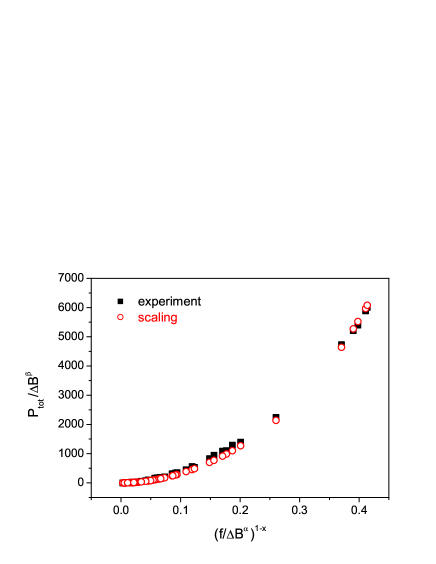
Figure 1: Projection of the measurement points and the scaling theory points (5)-(7) in $[f/(\triangle B^{\alpha})^{(1-x)},P_{tot}/(\triangle B^{\beta})]$ plane.

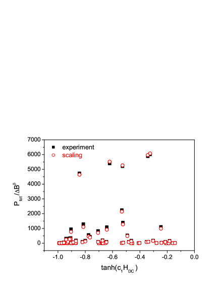
Figure 2: Projection of the measurement points and the scaling theory points (5)-(7) in $[tanh(H\,c_{1},P_{tot}/(\triangle B)^{\beta}]$ plane.

The B-H Loop measurements have been performed for SIFERRIT N87. The Core Losses per unit volume have been calculated as the enclosed area of the B-H loop, multiplied by the frequency f. The following factors influence the accuracy of measurements: 1) Phase Shift Error of Voltage and Current $<4\%$, 2) Equipment Accuracy $<5,6\%$, 3) Capacitive Couplings negligible (capacitive currents are relatively lower compared to inductive currents), and 4) Temperature $<4\%$. For details of the applied measurement method and the errors of the relevant factors we refer to (bib:Ecklebe, ), (bib:Ecklebe1, ). The parameter values of (4)-(7) have been estimated by minimization of $\chi^{2}$ using the Simplex method of Nelder and Mead (bib:pade, ) and the our experimental data. The measurement series consists of $60$ points, see TABLE 1. Standard deviation per point is equal to $15[\frac{W}{m^{3}T^{\beta}}]$ Applying the formulae (4)-(7) and the estimated parameter values TABLE 2 we have drawn the three scatter plots Fig. 1, Fig. 2 and Fig. 3, which compare estimated points with the experimental ones in the three projections, respectively. Note that, in order to prevent generation of large numbers in the estimation process the unit of frequency was kHz while other magnitudes were expressed in SI unit system.

Table 2: The set of estimated model’s parameters of (4)-(7) for $\delta=0$

$\alpha$	$\beta$	$x$	$\Gamma_{1}$	$\Gamma_{2}$	$\Gamma_{3}$	$\Gamma_{4}$	$\Gamma_{5}$
${\small-11,628}$	-8,6382	0,52629	-1,4083	739,55	1253,4	4238,5	0,12264
$\Gamma_{6}$	$\Gamma_{7}$	$\Gamma_{8}$	y	$\psi_{3}$	$c_{3}$	$\psi_{4}$	$\psi_{5}$
-30,972	-51,869	-4201,45	0,28877	14,4558	0,1648	-1,27E-01	0,28302
$c_{2}$	$\tau$	$\gamma$	$\psi_{2}$	$\psi_{1}$	$c_{1}$	$c_{0}$	z
-0,1808	7,77E-02	-0,17954	2,3966	-0,8993	-2,44E-02	-0,4877	4,84E-02

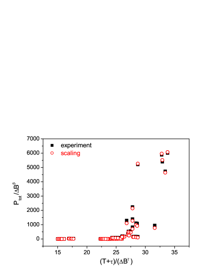
Figure 3: Projection of the measurement points and the scaling theory points (5)-(7) in $[\frac{T+\tau}{(\triangle B)^{\gamma}},P_{tot}/(\triangle B)^{\beta}]$ plane.

IV Conclusions

Efficiency of the scaling in solving problems concerning of power losses in Soft Magnetic Materials has been confirmed all ready in the recent papers (bib:Sokal1, )-(bib:Ruszcz, ). However, this paper is the first one which presents application of scaling in modeling of temperature dependence of the core loss. The presented method is universal, which means that it works for wide spectrum of expositions and different soft magnetic materials. Moreover the presented model formulae (4)-(7) are not closed and can be adapted for a current problem by fitting the forms of both factors $\Phi$ and $\Theta$. At the end one must say that success in applying the scaling depends on property of data. The data must obey the scaling.

References

- (1) C.P. Steinmetz, On the law of hysteresis, Trans. Amer. Inst. Elect. Eng., 9, 3-64 (1892).
- (2) M. Albach, T. Durbaum, and A. Brockmeyer, IEEE Power Electronics Specialists Conference, pp. 1463 1468 (1996).
- (3) J. Reinert, A. Brockmeyer J. Reinert, A. Brockmeyer, and R.W. De Doncker, Calculation of losses in ferro- and ferrimagnetic materials based on the modified Steinmetz equation, Annual Meeting of the IEEE Industry Applications Society, 1999.
- (4) Jieli Li, T. Abdallah, and C. R. Sullivan, Improved calculation of core loss with nonsinusoidal waveforms, in Annual Meeting of the IEEE Industry Applications Society, 2001, pp. 2203-2210.
- (5) K. Venkatachalam, C. R. Sullivan, T. Abdallah, and H. Tacca, Accurate prediction of ferrite core loss with nonsinusoidal waveforms using only Steinmetz parameters IEEE Workshop on Computers in Power Electronics (COMPEL), 2002.
- (6) Alex Van den Bossche, Vencislav Valchev, Georgi Georgiev, Measurement and loss model of ferrites in nonsinusoidal waves, IEEE Power Electronics Specialists Conference, 2004.
- (7) Jonas Mühlethaler, Jürgen Biela, Johann Walter Kolar and Andreas Ecklebe, Core-Loss Calculation for Magnetic Components Employed in Power Electronic Systems, IEEE TRANSACTIONS ON POWER ELECTRONICS, 27, pp.964-973 (2012).
- (8) J. Mühlethaler, J. Biela, J.W. Kolar, A. Ecklebe, Core Losses Under the DC Bias Condition Based on Steinmetz Parameters, IEEE Transactions on Power Electronics, 27, pp.953-963 (2012).
- (9) F. Fiorillo and A. Novikov, An improved approach to power lossess in magnetic laminations under nonsinusoidal induction waveform, IEEE Trans. Magnet., 26, pp.2559-2561 (1990).
- (10) K. Sokalski, J. Szczyg owski, M. Najgebauer and W. Wilczy nski, Thermodynamical Scaling of Eddy Current Losses in Magnetic Materials, Proc. 12th IGTE Symposium, 2006.
- (11) K. Sokalski, J. Szczygłowski, M. Najgebauer and W. Wilczyński, [12] K. Sokalski, J. Szczyg owski, M. Najgebauer and W. Wilczy nski, Losses scaling in soft magnetic materials, COMPEL: Int. J. Comput. Math. Electr. Electron. Eng.,26, 640-649 ( 2007), COMPEL: Int. J. Comput. Math. Electr. Electron. Eng.,26, 640-649 ( 2007).
- (12) K. Sokalski, J. Szczyg owski, and W. Wilczy nski, Scaling conception of power loss separation in soft magnetic materials, http://arxiv.org/abs/1111.0939v1.
- (13) A. Ruszczyk, K. Sokalski, J. Szczygłowski, Scaling in Modeling of Core Losses in Soft Magnetic Materials Exposed to Nonsinusoidal Flux Waveforms and DC Bias, SMM21 Conference, Budapest 2013.
- (14) J. Cale, S.D. Sudhoff, S. D. and R.R. Chan, A Field-Extrema Hysteresis Loss Model for High-Frequency Ferrimagnetic Materials, IEEE Transactions on Magnetics, vol. 44, issue 7, pp. 1728-1736 (2008).
- (15) K. Sokalski, J. Szczygłowski, ABB REPORT, PLCRC/50002437/02/1725/2011.
- (16) William H. Press, Saul A. Teukolsky, William T. Vetterling, Brian P. Flannery, Numerical Recipes in Fortran 77, The Art of Scientific Computing, Second Edition, Volume 1 of Fortran Numerical Recipes, Published by the Press Syndicate of the University of Cambridge 1997, p. 194.