11institutetext: CEA Saclay Nano-INNOV, CEA LIST, Laboratory for the Modelling and Analysis of Interacting Systems, Point Courrier 174, 91191 Gif sur Yvette CEDEX, {Eric.Goubault,Sylvie.Putot}@cea.fr

General Inner Approximation of Vector-valued Functions

Olivier Mullier    Éric Goubault    Michel Kieffer    Sylvie Putot    Olivier Mullier    Éric Goubault    Michel Kieffer and Sylvie Putot
Abstract

This paper addresses the problem of evaluating a subset of the range of a vector-valued function. It is based on a work by Goldsztejn and Jaulin which provides methods based on interval analysis to address this problem when the dimension of the domain and co-domain of the function are equal. This paper extends this result to vector-valued functions with domain and co-domain of different dimensions. This extension requires the knowledge of the rank of the Jacobian function on the whole domain. This leads to the sub-problem of extracting an interval sub-matrix of maximum rank from a given interval matrix. Three different techniques leading to approximate solutions of this extraction are proposed and compared.

1 Introduction

Computing the values a function can take over some domain is generally of great interest in the analysis of numerical programs as in abstract interpretation [3], in robust control of dynamic systems [11], or in global optimization [18]. Computing the image of a domain by a function (also called direct image or range) exactly is intractable in general. The classical solution is then to compute an outer approximation of this range, which can unfortunately be very pessimistic. This outer approximation may introduce many values which do not belong to the range. Providing, in addition, an inner approximation can be helpful to state the quality of the outer approximation.

For scalar-valued functions, an inner approximation can be evaluated using modal intervals [7] (using Kaucher arithmetic [12]) or twin arithmetic [16]. When f𝑓f maps nsuperscript𝑛\mathbb{R}^{n} to nsuperscript𝑛\mathbb{R}^{n}, modal intervals [4] can also be used in the linear case. For the non-linear case, set inversion [10] can be used when f𝑓f is globally invertible (when an inverse function f1superscript𝑓1f^{-1} can be produced).

In the more general case of f𝑓f being locally invertible, the method described by Goldsztejn and Jaulin in [5] can be applied. This technique requires however the inverse of the Jacobian of f𝑓f. Thus it can only be applied for functions from nsuperscript𝑛\mathbb{R}^{n} to nsuperscript𝑛\mathbb{R}^{n} of constant rank n𝑛n.

This paper proposes a generalization of the method in [5] to deal with functions f𝑓f from 𝒟m𝒟superscript𝑚\mathcal{D}\subseteq\mathbb{R}^{m} to nsuperscript𝑛\mathbb{R}^{n}, with mn𝑚𝑛m\neq n, with rank r𝑟r. It describes a method to compute an inner approximation for at most r𝑟r components of f𝑓f. As in [5], the evaluation of the Jacobian of the function on a given subset of its domain is needed. There, the identification of the components that can be used to compute an inner approximation has to be done by extracting the sub-matrix of full rank in its Jacobian. Checking regularity of interval matrices is a NP-hard problem [19], so is the problem of extracting an interval sub-matrix of full rank. To our knowledge, no necessary and sufficient condition for checking regularity can be used to address this problem (a list of necessary and sufficient conditions for an interval matrix to be regular can be found in [20]).

This paper is organized as follows: Section 2 recalls the main result of [5] on the computation of an inner approximation of the range of vector-valued functions with domain and co-domain of the same dimension. Section 3 describes the extension of this result to functions with domain and co-domain of different dimensions. Section 4 addresses algorithms for computing and inner approximation and describes how sub-matrices of full rank can be extracted from a given interval matrix using different techniques. The computation of an inner approximation of the range of functions is illustrated on examples in Section 5.

Notations

𝐱=[x¯,x¯]{x:x¯xx¯}𝐱¯𝑥¯𝑥conditional-set𝑥¯𝑥𝑥¯𝑥{\bf x}=\left[\underline{x},\overline{x}\right]\triangleq\{x\in\mathbb{R}:\underline{x}\leqslant x\leqslant\overline{x}\} is an interval where x¯¯𝑥\underline{x} and x¯¯𝑥\overline{x} are respectively its lower and its upper bound. 𝕀{[x¯,x¯]:x¯,x¯,x¯x¯}𝕀conditional-set¯𝑥¯𝑥formulae-sequence¯𝑥¯𝑥¯𝑥¯𝑥\mathbb{IR}\triangleq\{\left[\underline{x},\overline{x}\right]:\underline{x},\overline{x}\in\mathbb{R},\underline{x}\leqslant\overline{x}\} represents the set of intervals. A box is the Cartesian product of n𝑛n intervals in 𝕀n𝕀superscript𝑛\mathbb{IR}^{n}. For an interval 𝐱=[x¯,x¯]𝐱¯𝑥¯𝑥{\bf x}=\left[\underline{x},\overline{x}\right], the width is wid(𝐱)x¯x¯wid𝐱¯𝑥¯𝑥\text{wid}({\bf x})\triangleq\overline{x}-\underline{x}, the midpoint is mid(𝐱)12(x¯+x¯)mid𝐱12¯𝑥¯𝑥\text{mid}({\bf x})\triangleq\frac{1}{2}(\overline{x}+\underline{x}), the interior is int(𝐱){x|x¯<x<x¯}int𝐱conditional-set𝑥¯𝑥𝑥¯𝑥\operatorname{int}({\bf x})\triangleq\{x\in\mathbb{R}|\underline{x}<x<\overline{x}\}, and the boundary is denoted by 𝐱𝐱\partial{\bf x}. The magnitude is denoted |𝐱|max{|x¯|,|x¯|}𝐱¯𝑥¯𝑥|{\bf x}|\triangleq\max\{|\underline{x}|,|\overline{x}|\} and the mignitude is 𝐱min{|x¯|,|x¯|}delimited-⟨⟩𝐱¯𝑥¯𝑥\langle{\bf x}\rangle\triangleq\min\{|\underline{x}|,|\overline{x}|\} if 0𝐱0𝐱0\notin{\bf x} and 𝐱=0delimited-⟨⟩𝐱0\langle{\bf x}\rangle=0 otherwise. The width of an interval vector 𝐱𝕀n𝐱𝕀superscript𝑛{\bf x}\in\mathbb{IR}^{n} is max1in(wid(𝐱i))subscript1𝑖𝑛widsubscript𝐱𝑖\max_{1\leqslant i\leqslant n}(\text{wid}({\bf x}_{i})).

The core of interval analysis is its fundamental theorem (see, e.g., [15] or [17]) asserting that an evaluation of an expression using intervals gives an outer approximation of the range of this expression over the considered intervals. An interval function is an inclusion function denoted here 𝐟𝐟{\bf f}: f(𝐱)={f(x):x𝐱}𝐟(𝐱)𝑓𝐱conditional-set𝑓𝑥𝑥𝐱𝐟𝐱f({\bf x})=\{f(x):x\in{\bf x}\}\subseteq{\bf f}({\bf x}) for 𝐱𝐱{\bf x} included in the domain of f𝑓f. For an interval square matrix 𝐀𝕀n×n𝐀𝕀superscript𝑛𝑛{\bf A}\in\mathbb{IR}^{n\times n}, Diag𝐀𝕀n×nDiag𝐀𝕀superscript𝑛𝑛\operatorname{Diag}{\bf A}\in\mathbb{IR}^{n\times n} is the diagonal interval matrix whose diagonal entries are (Diag𝐀)ii=𝐀iisubscriptDiag𝐀𝑖𝑖subscript𝐀𝑖𝑖(\operatorname{Diag}{\bf A})_{ii}={\bf A}_{ii}, 1in1𝑖𝑛1\leqslant i\leqslant n, and 0 elsewhere. OffDiag𝐀𝕀n×nOffDiag𝐀𝕀superscript𝑛𝑛\operatorname{OffDiag}{\bf A}\in\mathbb{IR}^{n\times n} is the interval matrix with null diagonal and with off-diagonal entries such that (OffDiag𝐀)ij=𝐀ijsubscriptOffDiag𝐀𝑖𝑗subscript𝐀𝑖𝑗(\operatorname{OffDiag}{\bf A})_{ij}={\bf A}_{ij}. For a vector-valued function f:𝒟mn:𝑓𝒟superscript𝑚superscript𝑛f:\mathcal{D}\subseteq\mathbb{R}^{m}\rightarrow\mathbb{R}^{n} and x𝒟𝑥𝒟x\in\mathcal{D}, fi:j(x)(fi(x),fi+1(x),,fj(x))Tsubscript𝑓:𝑖𝑗𝑥superscriptsubscript𝑓𝑖𝑥subscript𝑓𝑖1𝑥subscript𝑓𝑗𝑥𝑇f_{{i:j}}(x)\triangleq(f_{i}(x),f_{i+1}(x),\dots,f_{j}(x))^{T} for ij𝑖𝑗i\leqslant j. For the Jacobian Jfsuperscript𝐽𝑓J^{f} of f𝑓f and x𝒟𝑥𝒟x\in\mathcal{D},

Jfi:j,xk:(x)(fixk(x)fixk+1(x)fix(x)fi+1xk(x)fi+1xk+1(x)fi+1x(x)fjxk(x)fjxk+1(x)fjx(x))superscript𝐽subscript𝑓:𝑖𝑗subscript𝑥:𝑘𝑥subscript𝑓𝑖subscript𝑥𝑘𝑥subscript𝑓𝑖subscript𝑥𝑘1𝑥subscript𝑓𝑖subscript𝑥𝑥subscript𝑓𝑖1subscript𝑥𝑘𝑥subscript𝑓𝑖1subscript𝑥𝑘1𝑥subscript𝑓𝑖1subscript𝑥𝑥missing-subexpressionsubscript𝑓𝑗subscript𝑥𝑘𝑥subscript𝑓𝑗subscript𝑥𝑘1𝑥subscript𝑓𝑗subscript𝑥𝑥J^{f_{i:j},x_{k:\ell}}(x)\triangleq\left(\begin{array}[]{cccc}\frac{\partial f_{i}}{\partial x_{k}}(x)&\frac{\partial f_{i}}{\partial x_{k+1}}(x)&\dots&\frac{\partial f_{i}}{\partial x_{\ell}}(x)\\ \frac{\partial f_{i+1}}{\partial x_{k}}(x)&\frac{\partial f_{i+1}}{\partial x_{k+1}}(x)&\dots&\frac{\partial f_{i+1}}{\partial x_{\ell}}(x)\\ \vdots&\vdots&\vdots\\ \frac{\partial f_{j}}{\partial x_{k}}(x)&\frac{\partial f_{j}}{\partial x_{k+1}}(x)&\dots&\frac{\partial f_{j}}{\partial x_{\ell}}(x)\end{array}\right)

is the restriction of the Jacobian of f𝑓f for ji𝑗𝑖j-i components of f𝑓f and k𝑘\ell-k components of x𝑥x. Ikk×ksubscript𝐼𝑘superscript𝑘𝑘I_{k}\in\mathbb{R}^{k\times k} is the identity matrix of dimension k𝑘k. The null matrix with k𝑘k rows and \ell columns is denoted 0k×subscript0𝑘0_{k\times\ell} and the null vector of k𝑘k entries is denoted 0k(0,,0)Tsubscript0𝑘superscript00𝑇0_{k}\triangleq(0,\dots,0)^{T}.

2 Inner approximation for functions with domain and co-domain of the same dimension

This section recalls the main result of [5] to evaluate an inner approximation of the range of a function with domain and co-domain of the same dimension.

Corollary 1

Let 𝐱𝕀n𝐱𝕀superscript𝑛{\bf x}\in\mathbb{IR}^{n} and f:𝐱n:𝑓𝐱superscript𝑛f:{\bf x}\rightarrow\mathbb{R}^{n} be a continuous function continuously differentiable in int(𝐱)int𝐱\operatorname{int}({\bf x}). Consider 𝐲𝕀n𝐲𝕀superscript𝑛{\bf y}\in\mathbb{IR}^{n} and x~𝐱~𝑥𝐱\tilde{x}\in{\bf x} such that f(x~)𝐲𝑓~𝑥𝐲f(\tilde{x})\in{\bf y}. Consider also an interval matrix 𝐉𝕀n×n𝐉𝕀superscript𝑛𝑛{\bf J}\in\mathbb{IR}^{n\times n} such that f(x)𝐉superscript𝑓𝑥𝐉f^{\prime}(x)\in{\bf J} for all x𝐱𝑥𝐱x\in{\bf x}. Assume that 0𝐉ii0subscript𝐉𝑖𝑖0\notin{\bf J}_{ii} for all i[1,,n]𝑖1𝑛i\in\left[1,\dots,n\right]. Let

H(𝐉,x~,𝐱,𝐲)=x~+(Diag1𝐉)(𝐲f(x~)(OffDiag𝐉)(𝐱x~))𝐻𝐉~𝑥𝐱𝐲~𝑥superscriptDiag1𝐉𝐲𝑓~𝑥OffDiag𝐉𝐱~𝑥H({\bf J},\tilde{x},{\bf x},{\bf y})=\tilde{x}+(\operatorname{Diag}^{-1}{\bf J})\Big{(}{\bf y}-f(\tilde{x})-(\operatorname{OffDiag}{\bf J})({\bf x}-\tilde{x})\Big{)} (1)

If H(𝐉,x~,𝐱,𝐲)int(𝐱)𝐻𝐉~𝑥𝐱𝐲int𝐱H({\bf J},\tilde{x},{\bf x},{\bf y})\subseteq\operatorname{int}({\bf x}) then 𝐲range(f,𝐱)𝐲range𝑓𝐱{\bf y}\subseteq\operatorname{range}(f,{\bf x}).

This corollary provides an efficient test for a box 𝐲𝐲{\bf y} to be a subset of the range of a vector-valued function. It can be used to compute an inner approximation of functions f𝑓f from nsuperscript𝑛\mathbb{R}^{n} to nsuperscript𝑛\mathbb{R}^{n}, see Section 4. The restriction on f𝑓f having same dimension of domain and co-domain comes from the matrix inversion of Diag𝐉Diag𝐉\operatorname{Diag}{\bf J} in (1).

Refer to caption𝐱𝐱{\bf x}𝐱~~𝐱\tilde{{\bf x}}x~~𝑥\tilde{x}fSsubscript𝑓𝑆f_{S}(fS)1superscriptsubscript𝑓𝑆1(f_{S})^{-1}𝐲~~𝐲\tilde{{\bf y}}x~+Γ(𝐉,𝐱~x~,𝐲~f(x~))~𝑥Γ𝐉~𝐱~𝑥~𝐲𝑓~𝑥\tilde{x}+\Gamma({\bf J},\tilde{{\bf x}}-\tilde{x},\tilde{{\bf y}}-f(\tilde{x}))fS(𝐱~)subscript𝑓𝑆~𝐱f_{S}(\tilde{{\bf x}})fS(𝐱)={f(x):x𝐱}subscript𝑓𝑆𝐱conditional-set𝑓𝑥𝑥𝐱f_{S}({\bf x})=\{f(x):x\in{\bf x}\}
Figure 1: Sets and functions involved in Corollary 1 for inner approximation.

Figure 1 illustrates the computation in Corollary 1. The left part of Figure 1 represents the domain 𝐱𝐱{\bf x} and the right part the co-domain of f𝑓f. The set-valued map fSsubscript𝑓𝑆f_{S} is defined from 𝒫(n)𝒫superscript𝑛\mathcal{P}(\mathbb{R}^{n}) (power set of nsuperscript𝑛\mathbb{R}^{n}) to 𝒫(n)𝒫superscript𝑛\mathcal{P}(\mathbb{R}^{n}) and returns the set {f(x):x𝒟}conditional-set𝑓𝑥𝑥𝒟\{f(x):x\in\mathcal{D}\} for a given set 𝒟𝒟\mathcal{D}, see [2]. From a given box 𝐱~𝐱~𝐱𝐱\tilde{{\bf x}}\subset{\bf x}, one wants to know if the box 𝐲~~𝐲\tilde{{\bf y}} computed by an inclusion function of f𝑓f over 𝐱~~𝐱\tilde{{\bf x}} belongs to the range of f𝑓f or equivalently if 𝐲~=𝐟(𝐱~)~𝐲𝐟~𝐱\tilde{{\bf y}}={\bf f}(\tilde{{\bf x}}) is a subset of fS(𝐱)subscript𝑓𝑆𝐱f_{S}({\bf x}). If 𝐱~~𝐱\tilde{{\bf x}} is too large compared to 𝐱𝐱{\bf x}, one might have 𝐲~=𝐟(𝐱~)fS(𝐱)~𝐲𝐟~𝐱not-subset-of-nor-equalssubscript𝑓𝑆𝐱\tilde{{\bf y}}={\bf f}(\tilde{{\bf x}})\nsubseteq f_{S}({\bf x}). To prove that 𝐲~fS(𝐱)~𝐲subscript𝑓𝑆𝐱\tilde{{\bf y}}\subset f_{S}({\bf x}), it is sufficient to prove that fS1(𝐲~)𝐱subscriptsuperscript𝑓1𝑆~𝐲𝐱f^{-1}_{S}(\tilde{{\bf y}})\subset{{\bf x}}. The function H(𝐉,x~,𝐱,𝐲)𝐻𝐉~𝑥𝐱𝐲H({\bf J},\tilde{x},{\bf x},{\bf y}) in (1) can be seen as an inclusion function for fS1fS(𝐱)subscriptsuperscript𝑓1𝑆subscript𝑓𝑆𝐱f^{-1}_{S}\circ f_{S}({\bf x}).

3 Extension for functions with domain and co-domain of different dimensions

Corollary 1 only applies for functions having the same dimension for domain and co-domain. It also needs that the determinant of the Jacobian is different from 0. Consider now the case of a function f𝑓f with domain and co-domain of different dimensions. In what follows, assume that f:𝒟mn:𝑓𝒟superscript𝑚superscript𝑛f:\mathcal{D}\subseteq\mathbb{R}^{m}\rightarrow\mathbb{R}^{n} is a C1superscript𝐶1C^{1} function of rank greater than or equal to r𝑟r on 𝒟𝒟\mathcal{D}. It is assumed that there exist r𝑟r components (xi1,,xir)subscript𝑥subscript𝑖1subscript𝑥subscript𝑖𝑟(x_{i_{1}},\dots,x_{i_{r}}) of x=(x1,,xm)𝒟m𝑥subscript𝑥1subscript𝑥𝑚𝒟superscript𝑚x=(x_{1},\dots,x_{m})\in\mathcal{D}\subseteq\mathbb{R}^{m} and r𝑟r components (fj1(x),,fjr(x))subscript𝑓subscript𝑗1𝑥subscript𝑓subscript𝑗𝑟𝑥(f_{j_{1}}(x),\dots,f_{j_{r}}(x)) such that

x𝒟m,det(fjkxi(x))1k,r0formulae-sequencefor-all𝑥𝒟superscript𝑚subscriptsubscript𝑓subscript𝑗𝑘subscript𝑥subscript𝑖𝑥formulae-sequence1𝑘𝑟0\forall x\in\mathcal{D}\subseteq\mathbb{R}^{m},\ \det\left(\frac{\partial f_{j_{k}}}{\partial x_{i_{\ell}}}(x)\right)_{1\leqslant k,\ell\leqslant r}\neq 0 (2)

Hereafter, without loss of generality, f𝑓f is considered after the permutation of the r𝑟r coordinates (xi1,,xir)subscript𝑥subscript𝑖1subscript𝑥subscript𝑖𝑟(x_{i_{1}},\dots,x_{i_{r}}) and the r𝑟r coordinates (fj1(x),,fjr(x))subscript𝑓subscript𝑗1𝑥subscript𝑓subscript𝑗𝑟𝑥(f_{j_{1}}(x),\dots,f_{j_{r}}(x)) (this permutation is discussed later in Section 4.3). It means that the Jacobian of f𝑓f has an r×r𝑟𝑟r\times r sub-matrix on the upper left such that

x𝒟m,det(fjxk(x))1j,kr0formulae-sequencefor-all𝑥𝒟superscript𝑚subscriptsubscript𝑓𝑗subscript𝑥𝑘𝑥formulae-sequence1𝑗𝑘𝑟0\forall x\in\mathcal{D}\subseteq\mathbb{R}^{m},\ \det\left(\frac{\partial f_{j}}{\partial x_{k}}(x)\right)_{1\leqslant j,k\leqslant r}\neq 0 (3)

Theorem 3.1 in [5] provides sufficient conditions for a box 𝐲𝐲{\bf y} to be included in the range of a function. Theorem 3.1 bellow generalizes this characterization by providing sufficient conditions for a box 𝐲1𝕀rsubscript𝐲1𝕀superscript𝑟{\bf y}_{1}\in\mathbb{IR}^{r} to be inside the projection on the first r𝑟r components of the image of f:𝒟mn:𝑓𝒟superscript𝑚superscript𝑛f:\mathcal{D}\subseteq\mathbb{R}^{m}\rightarrow\mathbb{R}^{n} when f𝑓f verifies (3).

Theorem 3.1

Let f:𝒟mn:𝑓𝒟superscript𝑚superscript𝑛f:\mathcal{D}\subseteq\mathbb{R}^{m}\rightarrow\mathbb{R}^{n} be a C1superscript𝐶1C^{1} function that verifies (3), 𝐮𝒟𝐮𝒟{\bf u}\subset\mathcal{D} a box in 𝕀m𝕀superscript𝑚\mathbb{IR}^{m} and 𝐲1𝕀rsubscript𝐲1𝕀superscript𝑟{\bf y}_{1}\in\mathbb{IR}^{r}. Assume that the two following conditions are satisfied

  1. (i)

    𝐲1f1:r(𝐮)=subscript𝐲1subscript𝑓:1𝑟𝐮{\bf y}_{1}\cap{f_{1:r}}(\partial{\bf u})=\emptyset;

  2. (ii)

    f1:r(u~)𝐲1subscript𝑓:1𝑟~𝑢subscript𝐲1{f_{1:r}}(\tilde{u})\in{\bf y}_{1} for some u~𝐮~𝑢𝐮\tilde{u}\in{\bf u},

then 𝐲1f1:r(𝐮)subscript𝐲1subscript𝑓:1𝑟𝐮{\bf y}_{1}\subseteq{f_{1:r}}({\bf u}).

Before starting the proof the next result is needed.

Lemma 1

Let f:𝒟n:𝑓𝒟superscript𝑛f:\mathcal{D}\rightarrow\mathbb{R}^{n} be a C1superscript𝐶1C^{1} function satisfying (3) and let E𝐸E be a compact such that E𝒟𝐸𝒟E\subset\mathcal{D}. Then one has (f1:r(E))f1:r(E)subscript𝑓:1𝑟𝐸subscript𝑓:1𝑟𝐸\partial(f_{1:r}(E))\subseteq f_{1:r}(\partial E).

Proof

Consider any y1(f1:r(E))subscript𝑦1subscript𝑓:1𝑟𝐸y_{1}\in\partial(f_{1:r}(E)). As f𝑓f is continuous, f1:rsubscript𝑓:1𝑟{f_{1:r}} is continuous as well. Then the image of E𝐸E, compact, by f1:rsubscript𝑓:1𝑟{f_{1:r}} is also compact. In particular it is closed so (f1:r(E))subscript𝑓:1𝑟𝐸\partial({f_{1:r}}(E)) is included in f1:r(E)subscript𝑓:1𝑟𝐸{f_{1:r}}(E). So there exists xE𝑥𝐸x\in E such that y1=f1:r(x)subscript𝑦1subscript𝑓:1𝑟𝑥y_{1}=f_{1:r}(x). Now suppose that xintE𝑥int𝐸x\in\operatorname{int}E. We now prove that this leads to a contradiction. As xintE𝑥int𝐸x\in\operatorname{int}E, there exists U𝑈U open of E𝐸E with xU𝑥𝑈x\in U. Because of (3), f1:rsubscript𝑓:1𝑟{f_{1:r}} is a submersion and as submersions are open maps (see [23]), V=f1:r(U)𝑉subscript𝑓:1𝑟𝑈V=f_{1:r}(U) is open in rsuperscript𝑟\mathbb{R}^{r}. We have y1Vsubscript𝑦1𝑉y_{1}\in V then y1intf1:r(E)subscript𝑦1intsubscript𝑓:1𝑟𝐸y_{1}\in\operatorname{int}f_{1:r}(E) which contradicts y1(f1:r(E))subscript𝑦1subscript𝑓:1𝑟𝐸y_{1}\in\partial(f_{1:r}(E)). As a conclusion we have xE𝑥𝐸x\in\partial E and eventually, (f1:r(E))f1:r(E)subscript𝑓:1𝑟𝐸subscript𝑓:1𝑟𝐸\partial(f_{1:r}(E))\subseteq f_{1:r}(\partial E).

Proof (Theorem 3.1)

𝐮𝐮{\bf u} is a compact of 𝒟𝒟\mathcal{D} and f𝑓f is a C1superscript𝐶1C^{1} function that verifies (3) so we have, from Lemma 1, (f1:r(𝐮))f1:r(𝐮)subscript𝑓:1𝑟𝐮subscript𝑓:1𝑟𝐮\partial({f_{1:r}}({\bf u}))\subseteq{f_{1:r}}(\partial{\bf u}). So 𝐲1(f1:r(𝐮))𝐲1f1:r(𝐮)=subscript𝐲1subscript𝑓:1𝑟𝐮subscript𝐲1subscript𝑓:1𝑟𝐮{\bf y}_{1}\cap\partial({f_{1:r}}({\bf u}))\subseteq{\bf y}_{1}\cap{f_{1:r}}(\partial{\bf u})=\emptyset therefore

𝐲1(f1:r(𝐮))=.subscript𝐲1subscript𝑓:1𝑟𝐮{\bf y}_{1}\cap\partial(f_{1:r}({\bf u}))=\emptyset. (4)

The set f1:r(𝐮)subscript𝑓:1𝑟𝐮{f_{1:r}}({\bf u}) is compact because 𝐮𝐮{\bf u} is compact and f1:rsubscript𝑓:1𝑟{f_{1:r}} is continuous. Let u~~𝑢\tilde{u} and y1=f1:r(u~)𝐲1subscript𝑦1subscript𝑓:1𝑟~𝑢subscript𝐲1y_{1}={f_{1:r}}(\tilde{u})\in{\bf y}_{1} be given in (ii𝑖𝑖ii). As the intersection of 𝐲1subscript𝐲1{\bf y}_{1} and f1:r(𝐮)subscript𝑓:1𝑟𝐮\partial{f_{1:r}}({\bf u}) is empty by (4), y1intf1:r(𝐮)subscript𝑦1intsubscript𝑓:1𝑟𝐮y_{1}\in\operatorname{int}{f_{1:r}}({\bf u}). Consider any z𝐲1𝑧subscript𝐲1z\in{\bf y}_{1} and suppose that zf1:r(𝐮)𝑧subscript𝑓:1𝑟𝐮z\notin{f_{1:r}}({\bf u}). Since 𝐲1subscript𝐲1{\bf y}_{1} is path connected, there exists a path included in 𝐲1subscript𝐲1{\bf y}_{1} between y1subscript𝑦1y_{1} and z𝑧z such that, by Lemma A.1. in [5], this path intersects f1:r(𝐮)subscript𝑓:1𝑟𝐮\partial{f_{1:r}}({\bf u}) which is not possible from (4). Therefore zf1:r(𝐮)𝑧subscript𝑓:1𝑟𝐮z\in{f_{1:r}}({\bf u}) which concludes the proof.

Theorem 3.1 is a generalization of Theorem 3.1 in [5] for a function satisfying (3). In Theorem 3.1 in [5], the set Σ={xint𝐱|detf(x)=0}Σconditional-set𝑥int𝐱superscript𝑓𝑥0\Sigma=\{x\in\operatorname{int}{{\bf x}}\ |\ \det f^{\prime}(x)=0\} can be extended for f1:rsubscript𝑓:1𝑟{f_{1:r}} by Σ2={xint𝐱|rank(f1:r(x))<r}subscriptΣ2conditional-set𝑥int𝐱ranksubscript𝑓:1𝑟𝑥𝑟\Sigma_{2}=\{x\in\operatorname{int}{{\bf x}}\ |\ \text{rank}({f_{1:r}}(x))<r\}. Due to (3), one has Σ2=subscriptΣ2\Sigma_{2}=\emptyset. In what follows, Corollary 2 of Theorem 3.1, which extends the inclusion test of Corollary 1, is introduced.

Corollary 2

Let f:𝒟mn:𝑓𝒟superscript𝑚superscript𝑛f:\mathcal{D}\subseteq\mathbb{R}^{m}\rightarrow\mathbb{R}^{n} be a C1superscript𝐶1C^{1} function that satisfies (3) and 𝐮=(𝐮1,𝐮2)𝕀r×𝕀mr𝐮subscript𝐮1subscript𝐮2𝕀superscript𝑟𝕀superscript𝑚𝑟{\bf u}=({\bf u}_{1},{\bf u}_{2})\in\mathbb{IR}^{r}\times\mathbb{IR}^{m-r}. Consider 𝐲1𝕀rsubscript𝐲1𝕀superscript𝑟{\bf y}_{1}\in\mathbb{IR}^{r}, u~=(u~1,u~2)(𝐮1,𝐮2)~𝑢subscript~𝑢1subscript~𝑢2subscript𝐮1subscript𝐮2\tilde{u}=(\tilde{u}_{1},\tilde{u}_{2})\in({\bf u}_{1},{\bf u}_{2}) such that f1:r(u~)𝐲1subscript𝑓:1𝑟~𝑢subscript𝐲1{f_{1:r}}(\tilde{u})\in{\bf y}_{1} and 𝐉f1:r=(𝐉f1:r,u1𝐉f1:r,u2)𝕀r×msuperscript𝐉subscript𝑓:1𝑟superscript𝐉subscript𝑓:1𝑟subscript𝑢1superscript𝐉subscript𝑓:1𝑟subscript𝑢2𝕀superscript𝑟𝑚{\bf J}^{f_{1:r}}=\left({\bf J}^{{f_{1:r}},u_{1}}\ {\bf J}^{{f_{1:r}},u_{2}}\right)\in\mathbb{IR}^{r\times m} an interval matrix containing Jf1:rsuperscript𝐽subscript𝑓:1𝑟J^{f_{1:r}} the Jacobian of f1:rsubscript𝑓:1𝑟{f_{1:r}} on (𝐮1,𝐮2)subscript𝐮1subscript𝐮2({\bf u}_{1},{\bf u}_{2}) such that 0(𝐉f1:r,u1)ii0subscriptsuperscript𝐉subscript𝑓:1𝑟subscript𝑢1𝑖𝑖0\notin\left({\bf J}^{{f_{1:r}},u_{1}}\right)_{ii} for 1ir1𝑖𝑟1\leqslant i\leqslant r. Let

Hf1:r(𝐉f1:r,u~,𝐮,𝐲1)=u~1+(Diag1𝐉f1:r,u1)×\displaystyle H_{f_{1:r}}({\bf J}^{f_{1:r}},\tilde{u},{\bf u},{\bf y}_{1})=\tilde{u}_{1}+(\operatorname{Diag}^{-1}{\bf J}^{{f_{1:r}},u_{1}})\times
(𝐲1f1:r(u~)(OffDiag𝐉f1:r,u1)(𝐮1u~1)𝐉f1:r,u2(𝐮2u~2)).subscript𝐲1subscript𝑓:1𝑟~𝑢OffDiagsuperscript𝐉subscript𝑓:1𝑟subscript𝑢1subscript𝐮1subscript~𝑢1superscript𝐉subscript𝑓:1𝑟subscript𝑢2subscript𝐮2subscript~𝑢2\displaystyle\Big{(}{\bf y}_{1}-{f_{1:r}}(\tilde{u})-(\operatorname{OffDiag}{\bf J}^{{f_{1:r}},u_{1}})({\bf u}_{1}-\tilde{u}_{1})-{\bf J}^{{f_{1:r}},u_{2}}({\bf u}_{2}-\tilde{u}_{2})\Big{)}.

If

Hf1:r(𝐉f1:r,u~,𝐮,𝐲1)int(𝐮1),subscript𝐻subscript𝑓:1𝑟superscript𝐉subscript𝑓:1𝑟~𝑢𝐮subscript𝐲1intsubscript𝐮1H_{f_{1:r}}({\bf J}^{f_{1:r}},\tilde{u},{\bf u},{\bf y}_{1})\subseteq\operatorname{int}({\bf u}_{1}), (5)

then

𝐲1f1:r(𝐮).subscript𝐲1subscript𝑓:1𝑟𝐮{\bf y}_{1}\subseteq{f_{1:r}}({\bf u}).
Proof

It is sufficient to prove that if (5) is satisfied, the conditions of Theorem 3.1 are satisfied too.

(i𝑖i) Let u=(u1,u2)𝐮𝑢subscript𝑢1subscript𝑢2𝐮u=(u_{1},u_{2})\in\partial{\bf u}. Since u𝐮𝑢𝐮u\in{\bf u}, the mean value theorem applied to f1:rsubscript𝑓:1𝑟f_{1:r} (see [17]) shows that

f1:r(u)f1:r(u~)+𝐉f1:r(𝐮u~)subscript𝑓:1𝑟𝑢subscript𝑓:1𝑟~𝑢superscript𝐉subscript𝑓:1𝑟𝐮~𝑢{f_{1:r}}(u)\in{f_{1:r}}(\tilde{u})+{\bf J}^{{f_{1:r}}}({\bf u}-\tilde{u}) (6)

Let us show that f1:r(u~)+𝐉f1:r(𝐮u~)𝐲1subscript𝑓:1𝑟~𝑢superscript𝐉subscript𝑓:1𝑟𝐮~𝑢subscript𝐲1{f_{1:r}}(\tilde{u})+{\bf J}^{{f_{1:r}}}({\bf u}-\tilde{u})\cap{\bf y}_{1}\neq\emptyset which implies (i)𝑖(i) false contradicts (5). Assume that there exists J𝐉f1:r𝐽superscript𝐉subscript𝑓:1𝑟J\in{\bf J}^{{f_{1:r}}}, J=(J1J2)𝐽subscript𝐽1subscript𝐽2J=(J_{1}J_{2}) with J1r×rsubscript𝐽1superscript𝑟𝑟J_{1}\in\mathbb{R}^{r\times r} and J2r×mrsubscript𝐽2superscript𝑟𝑚𝑟J_{2}\in\mathbb{R}^{r\times m-r}; u=(u1,u2)T𝑢superscriptsubscript𝑢1subscript𝑢2𝑇u=(u_{1},u_{2})^{T}, u~=(u~1,u~2)T~𝑢superscriptsubscript~𝑢1subscript~𝑢2𝑇\tilde{u}=(\tilde{u}_{1},\tilde{u}_{2})^{T}, and y1𝐲1subscript𝑦1subscript𝐲1y_{1}\in{\bf y}_{1} such that

y1subscript𝑦1\displaystyle y_{1} =\displaystyle= f1:r(u~)+J(uu~)subscript𝑓:1𝑟~𝑢𝐽𝑢~𝑢\displaystyle{f_{1:r}}(\tilde{u})+J(u-\tilde{u}) (7)
=\displaystyle= f1:r(u~)+J1(u1u~1)+J2(u2u~2)subscript𝑓:1𝑟~𝑢subscript𝐽1subscript𝑢1subscript~𝑢1subscript𝐽2subscript𝑢2subscript~𝑢2\displaystyle{f_{1:r}}(\tilde{u})+J_{1}(u_{1}-\tilde{u}_{1})+J_{2}(u_{2}-\tilde{u}_{2})

By splitting J1subscript𝐽1J_{1} in DiagJ1+OffDiagJ1Diagsubscript𝐽1OffDiagsubscript𝐽1\operatorname{Diag}J_{1}+\operatorname{OffDiag}J_{1} in (7), we obtain:

y1f1:r(u~)J2(u2u~2)=(DiagJ1)(u1u~1)+(OffDiagJ1)(u1u~1)subscript𝑦1subscript𝑓:1𝑟~𝑢subscript𝐽2subscript𝑢2subscript~𝑢2Diagsubscript𝐽1subscript𝑢1subscript~𝑢1OffDiagsubscript𝐽1subscript𝑢1subscript~𝑢1y_{1}-{f_{1:r}}(\tilde{u})-J_{2}(u_{2}-\tilde{u}_{2})=(\operatorname{Diag}J_{1})(u_{1}-\tilde{u}_{1})+(\operatorname{OffDiag}J_{1})(u_{1}-\tilde{u}_{1})
u~1+(Diag1J1)(y1f1:r(u~)(OffDiagJ1)(u1u~1)J2(u2u~2))=u1subscript~𝑢1superscriptDiag1subscript𝐽1subscript𝑦1subscript𝑓:1𝑟~𝑢OffDiagsubscript𝐽1subscript𝑢1subscript~𝑢1subscript𝐽2subscript𝑢2subscript~𝑢2subscript𝑢1\tilde{u}_{1}+(\operatorname{Diag}^{-1}J_{1})\left(y_{1}-{f_{1:r}}(\tilde{u})-(\operatorname{OffDiag}J_{1})(u_{1}-\tilde{u}_{1})-J_{2}(u_{2}-\tilde{u}_{2})\right)=u_{1}

As u𝐮𝑢𝐮u\in{\bf u}, y1𝐲1subscript𝑦1subscript𝐲1y_{1}\in{\bf y}_{1}, Diag1J1Diag1𝐉1superscriptDiag1subscript𝐽1superscriptDiag1subscript𝐉1\operatorname{Diag}^{-1}J_{1}\in\operatorname{Diag}^{-1}{\bf J}_{1}, OffDiagJ1OffDiag𝐉1OffDiagsubscript𝐽1OffDiagsubscript𝐉1\operatorname{OffDiag}J_{1}\in\operatorname{OffDiag}{\bf J}_{1}, and J2𝐉2subscript𝐽2subscript𝐉2J_{2}\in{\bf J}_{2}, one gets

u1Hf1:r((𝐉1𝐉2),u~,𝐮,𝐲1)subscript𝑢1subscript𝐻subscript𝑓:1𝑟subscript𝐉1subscript𝐉2~𝑢𝐮subscript𝐲1u_{1}\in H_{f_{1:r}}(({\bf J}_{1}\ {\bf J}_{2}),\tilde{u},{\bf u},{\bf y}_{1}) (8)

and u1𝐮1subscript𝑢1subscript𝐮1u_{1}\in\partial{\bf u}_{1} which contradicts (5). Then (5) implies (i)𝑖(i).

(ii)𝑖𝑖(ii) By hypothesis, f1:r(u~)𝐲1subscript𝑓:1𝑟~𝑢subscript𝐲1{f_{1:r}}(\tilde{u})\in{\bf y}_{1}.

For a function f:𝒟mn:𝑓𝒟superscript𝑚superscript𝑛f:\mathcal{D}\subseteq\mathbb{R}^{m}\rightarrow\mathbb{R}^{n}, Corollary 2 gives a test for a box to belong to the image of r𝑟r components of f𝑓f. It can only be performed if the Jacobian for r𝑟r components of the function evaluated over the considered box is of full rank r𝑟r. When the rank of f𝑓f equals the dimension of the co-domain, f𝑓f is a submersion [1], Corollary 2 can be used to compute an inner approximation of the entire range of f𝑓f.

Example 1

Let f:𝒟3:𝑓𝒟superscript3f:\mathcal{D}\subset\mathbb{R}\rightarrow\mathbb{R}^{3} be a function that satisfies (3) for r=1𝑟1r=1.

f::𝑓absent\displaystyle f: 𝐱3𝐱superscript3\displaystyle{\bf x}\subset\mathbb{R}\rightarrow\mathbb{R}^{3} (12)
x(sin2xsinxx2)maps-to𝑥2𝑥𝑥𝑥2\displaystyle x\mapsto\left(\begin{array}[]{c}\sin 2x\\ \sin x\\ \frac{x}{2}\end{array}\right)

The box 𝐱=[0,π]𝒟𝐱0𝜋𝒟{\bf x}=\left[0,\pi\right]\subset\mathcal{D} is considered as the domain on which f𝑓f is studied. The function is of constant rank 1 then using Corollary 2, one is able to compute an inner approximation of the range of a single component of f𝑓f e.g. f1(𝐱)subscript𝑓1𝐱f_{1}({\bf x}), f2(𝐱)subscript𝑓2𝐱f_{2}({\bf x}) or f3(𝐱)subscript𝑓3𝐱f_{3}({\bf x}).

Refer to captionf3(x)subscript𝑓3𝑥f_{3}(x)f2(x)subscript𝑓2𝑥f_{2}(x)f1(x)subscript𝑓1𝑥f_{1}(x)f(𝐱)𝑓𝐱f({\bf x})
Figure 2: Example for f:(𝐱)3:𝑓𝐱maps-tosuperscript3f:({\bf x})\subseteq\mathbb{R}\mapsto\mathbb{R}^{3} of constant rank 1.

There is of course no proper box of dimension 2 or 3 included in the range of f𝑓f. Figure 2 represents the range of the function defined in (12).

4 Algorithms

4.1 When domain and co-domain have the same dimension

Algorithm 1 in [5] computes an inner approximation for functions with domain and co-domain of the same dimension using Corollary 1 and a bisection algorithm. The method is as follows. For a given box 𝐱~~𝐱\tilde{{\bf x}} included in the initial domain 𝐱𝐱{\bf x}, a box 𝐲~~𝐲\tilde{{\bf y}} such that f(𝐱)={f(x):x𝐱~}𝐲~𝑓𝐱conditional-set𝑓𝑥𝑥~𝐱~𝐲f({\bf x})=\{f(x):x\in\tilde{{\bf x}}\}\subseteq\tilde{{\bf y}} is computed using the interval extension 𝐟𝐟{\bf f} of f𝑓f.

If the hypotheses of Corollary 1 are satisfied, 𝐲~~𝐲\tilde{{\bf y}} is part of an inner approximation of the range of f𝑓f. If they are not satisfied, 𝐱~~𝐱\tilde{{\bf x}} is partitioned into two smaller boxes 𝐱~superscript~𝐱\tilde{{\bf x}}^{\prime} and 𝐱~′′superscript~𝐱′′\tilde{{\bf x}}^{\prime\prime} that are treated like 𝐱~~𝐱\tilde{{\bf x}} was. If the box 𝐱~=(𝐱~1,,𝐱~m)~𝐱subscript~𝐱1subscript~𝐱𝑚\tilde{{\bf x}}=(\tilde{{\bf x}}_{1},\dots,\tilde{{\bf x}}_{m}) is deemed too small to be further bisected (i.e. when wid(𝐱)<εwid𝐱𝜀\text{wid}({\bf x})<\varepsilon where ε𝜀\varepsilon is a user-defined parameter), then the iterations stop for this box. This is described in Algorithm 1. It uses the function Inner described in Algorithm 2, to decide if a box belongs to the range of a function.

Input: f𝑓f, 𝐱𝐱{\bf x}, ϵitalic-ϵ\epsilon
Output: InsidesubscriptInside\mathcal{L}_{\texttt{Inside}} (list of boxes), BoundarysubscriptBoundary\mathcal{L}_{\texttt{Boundary}} (list of boxes)
1 InsidesubscriptInside\mathcal{L}_{\texttt{Inside}}: empty list of boxes;
2 DomainsubscriptDomain\mathcal{L}_{\texttt{Domain}}: empty list of boxes (sorted by decreasing width);
3 DomainDomain{𝐱}subscriptDomainsubscriptDomain𝐱\mathcal{L}_{\texttt{Domain}}\leftarrow\mathcal{L}_{\texttt{Domain}}\cup\{{\bf x}\};
4 while DomainsubscriptDomain\mathcal{L}_{\texttt{Domain}} not empty do
5       𝐱~~𝐱absent\tilde{{\bf x}}\leftarrow Extract(DomainsubscriptDomain\mathcal{L}_{\texttt{Domain}});
       𝐲~𝐟(𝐱)(𝐟(mid(𝐱~))+𝐟(𝐱~)(𝐱~mid(𝐱~)))~𝐲𝐟𝐱𝐟mid~𝐱superscript𝐟~𝐱~𝐱mid~𝐱\tilde{{\bf y}}\leftarrow{\bf f}({\bf x})\cap({\bf f}(\text{mid}(\tilde{{\bf x}}))+{\bf f}^{\prime}(\tilde{{\bf x}})(\tilde{{\bf x}}-\text{mid}(\tilde{{\bf x}})));// Inclusion function
6       if Inner(f(f, 𝐱𝐱{\bf x}, 𝐱~~𝐱\tilde{{\bf x}}, 𝐲~)\tilde{{\bf y}}) then
            // Inner is from Algorithm 2 or Algorithm 3 according to the dimension of domain and co-domain
7             InsideInside{𝐲~}subscriptInsidesubscriptInside~𝐲\mathcal{L}_{\texttt{Inside}}\leftarrow\mathcal{L}_{\texttt{Inside}}\cup\{\tilde{{\bf y}}\};
8            
9       else if wid(𝐱~)ϵ~𝐱italic-ϵ(\tilde{{\bf x}})\geq\epsilon then
10             Bisect the box 𝐱~~𝐱\tilde{{\bf x}} to obtain 𝐱~superscript~𝐱\tilde{{\bf x}}^{\prime} and 𝐱~′′superscript~𝐱′′\tilde{{\bf x}}^{\prime\prime};
11             DomainDomain{𝐱~,𝐱~′′}subscriptDomainsubscriptDomainsuperscript~𝐱superscript~𝐱′′\mathcal{L}_{\texttt{Domain}}\leftarrow\mathcal{L}_{\texttt{Domain}}\cup\{\tilde{{\bf x}}^{\prime},\tilde{{\bf x}}^{\prime\prime}\};
12            
13       else
14             BoundaryBoundary{𝐲~}subscriptBoundarysubscriptBoundary~𝐲\mathcal{L}_{\texttt{Boundary}}\leftarrow\mathcal{L}_{\texttt{Boundary}}\cup\{\tilde{{\bf y}}\};
15            
16       end if
17      
18 end while
19return (Inside,Boundary)subscriptInsidesubscriptBoundary(\mathcal{L}_{\texttt{Inside}},\mathcal{L}_{\texttt{Boundary}});
Algorithm 1 Range inner-approximation evaluation algorithm as defined in [5].

Algorithm 2 decides for a given box 𝐱~𝐱~𝐱𝐱\tilde{{\bf x}}\subset{\bf x} whether 𝐟(𝐱~)𝐟~𝐱{\bf f}(\tilde{{\bf x}}) belongs to the range of f𝑓f over 𝐱𝐱{\bf x}. The parameters τ𝜏\tau and μ𝜇\mu are used for the domain inflation (see Section 5.2 in [5]) and C𝐶C is used to precondition the interval matrix 𝐉fsuperscript𝐉𝑓{\bf J}^{f} (see Section 4 in [5]).

Input: f𝑓f, 𝐱𝐱{\bf x}, 𝐱~~𝐱\tilde{{\bf x}}, 𝐲𝐲{\bf y}
Output: Boolean
1 τ1.01𝜏1.01\tau\leftarrow 1.01; μ0.9𝜇0.9\mu\leftarrow 0.9;
2 k0𝑘0k\leftarrow 0;
3 x~mid(𝐱~)~𝑥mid~𝐱\tilde{x}\leftarrow\text{mid}(\tilde{{\bf x}});
4 Cf(x~)1𝐶superscript𝑓superscript~𝑥1C\leftarrow f^{\prime}(\tilde{x})^{-1};
5 𝐛Cy~Cf(x~)𝐛𝐶~𝑦𝐶𝑓~𝑥{\bf b}\leftarrow C\tilde{y}-Cf(\tilde{x});
6 dk+subscript𝑑𝑘d_{k}\leftarrow+\infty; dk1+subscript𝑑𝑘1d_{k-1}\leftarrow+\infty;
7 while dkμdk1𝐱~𝐱subscript𝑑𝑘𝜇subscript𝑑𝑘1~𝐱𝐱d_{k}\leq\mu d_{k-1}\wedge\tilde{{\bf x}}\subseteq{\bf x} do
       𝐮Γ(C𝐟(𝐱~),𝐱~,x~,𝐛)𝐮Γ𝐶superscript𝐟~𝐱~𝐱~𝑥𝐛{\bf u}\leftarrow\Gamma(C{\bf f}^{\prime}(\tilde{{\bf x}}),\tilde{{\bf x}},-\tilde{x},{\bf b});// ΓΓ\Gamma is as defined in Corollary 1
8       if x~+𝐮𝐱~~𝑥𝐮~𝐱\tilde{x}+{\bf u}\subseteq\tilde{{\bf x}} then  return true;
9       ;
10       dk1dksubscript𝑑𝑘1subscript𝑑𝑘d_{k-1}\leftarrow d_{k};
       dkd(𝐱~,x~+τ𝐮)subscript𝑑𝑘𝑑~𝐱~𝑥𝜏𝐮d_{k}\leftarrow d(\tilde{{\bf x}},\tilde{x}+\tau{\bf u});// Domain inflation (Cf. Section 5.2 in [5])
11       𝐱~x~+τ𝐮~𝐱~𝑥𝜏𝐮\tilde{{\bf x}}\leftarrow\tilde{x}+\tau{\bf u};
12      
13 end while
14return false;
Algorithm 2 Inclusion test as defined in [5].
Example 2

Let f(x)=Ax𝑓𝑥𝐴𝑥f(x)=Ax with A=(1111),𝐴1111,A=\left(\begin{array}[]{rc}1&1\\ -1&1\end{array}\right)\text{,} and an initial domain 𝐱=([2,2],[2,2])𝐱2222{\bf x}=\left(\left[-2,2\right],\left[-2,2\right]\right). The aim is to compute an inner approximation of the set {f(x):x𝐱}conditional-set𝑓𝑥𝑥𝐱\{f(x):x\in{\bf x}\}. Of course, in this too simple case, direct methods would be applicable since A𝐴A is an invertible matrix, but this is intended to exemplify the method.

Refer to caption
Figure 3: Inner approximation of the range of f(x)=Ax𝑓𝑥𝐴𝑥f(x)=Ax when x[2,2]2𝑥superscript222x\in\left[-2,2\right]^{2} : BoundarysubscriptBoundary\mathcal{L}_{\texttt{Boundary}} (in black) and InsidesubscriptInside\mathcal{L}_{\texttt{Inside}} are evaluated using Algorithm 1 with ε=103𝜀superscript103\varepsilon=10^{-3}

Figure 3 shows the result obtained using Algorithm 1. Since bisections occur in the domain, the result consists of a set of overlapping boxes, obtained by an inclusion function computing outer approximations. Dark areas in Figure 3 indicate many overlapping boxes.

4.2 When the domain and co-domain have different dimensions

We now extend the method in [5] to compute an inner approximation of the projection on r𝑟r components of f𝑓f. Algorithm 1 is used unchanged, except for the inner inclusion test Inner in Line 7 which is now implemented by Algorithm 3 instead of Algorithm 2.

Input: f:𝒟mn:𝑓𝒟superscript𝑚superscript𝑛f:\mathcal{D}\subseteq\mathbb{R}^{m}\rightarrow\mathbb{R}^{n}, 𝐱𝐱{\bf x}, 𝐱superscript𝐱{\bf x}^{\prime}, 𝐲,r𝐲𝑟{\bf y},r// r𝑟r is the rank of f𝑓f
1
Output: Boolean
2 τ1.01𝜏1.01\tau\leftarrow 1.01; μ0.9𝜇0.9\mu\leftarrow 0.9;
3 k0𝑘0k\leftarrow 0;
4 x~mid(𝐱~)~𝑥mid~𝐱\tilde{x}\leftarrow\text{mid}(\tilde{{\bf x}});
5 𝐉f(𝐱)𝐉superscript𝑓𝐱{\bf J}\leftarrow f^{\prime}({\bf x});
Jf1:rsuperscript𝐽subscript𝑓:1𝑟absentJ^{{f_{1:r}}}\leftarrow transformation(f(x~),r)superscript𝑓~𝑥𝑟(f^{\prime}(\tilde{x}),r); // recovery of the r𝑟r first lines of the Jacobian of f𝑓f
C precondition(Jf1:r)𝐶 preconditionsuperscript𝐽subscript𝑓:1𝑟C\leftarrow\text{ precondition}(J^{f_{1:r}});// Computation of the precondition matrix
6 (u1~,u2~)~subscript𝑢1~subscript𝑢2absent(\tilde{u_{1}},\tilde{u_{2}})\leftarrow Extract(x~,r,m)~𝑥𝑟𝑚(\tilde{x},r,m);
7 (𝐮1~,𝐮2~)~subscript𝐮1~subscript𝐮2absent(\tilde{{\bf u}_{1}},\tilde{{\bf u}_{2}})\leftarrow Extract(𝐱~,r,m)~𝐱𝑟𝑚(\tilde{{\bf x}},r,m);
8 (𝐮1,𝐮2)subscript𝐮1subscript𝐮2absent({\bf u}_{1},{\bf u}_{2})\leftarrow Extract(𝐱,r,m)𝐱𝑟𝑚({\bf x},r,m);
9 (𝐉f1:r,u1,𝐉f1:r,u2)superscript𝐉subscript𝑓:1𝑟subscript𝑢1superscript𝐉subscript𝑓:1𝑟subscript𝑢2absent({\bf J}^{{f_{1:r}},u_{1}},{\bf J}^{{f_{1:r}},u_{2}})\leftarrow Extract(C𝐉,r,m)𝐶𝐉𝑟𝑚(C{\bf J},r,m);
𝐛(Cy~Cf(x~))1:r𝐛subscript𝐶~𝑦𝐶𝑓~𝑥:1𝑟{\bf b}\leftarrow\left(C\tilde{y}-Cf(\tilde{x})\right)_{1:r};// We need only the r𝑟r first components
10 dk+subscript𝑑𝑘d_{k}\leftarrow+\infty; dk1+subscript𝑑𝑘1d_{k-1}\leftarrow+\infty;
11 while dkμdk1𝐮~𝐮subscript𝑑𝑘𝜇subscript𝑑𝑘1~𝐮𝐮d_{k}\leq\mu d_{k-1}\wedge\tilde{{\bf u}}\subseteq{\bf u} do
12       𝐭(Diag 1𝐉f1:r,u1)(𝐲1f1:r(u~1,u~2)(OffDiag 𝐉f1:r,u1)(𝐮~1u~1)𝐉f1:r,u2(𝐮~2u~2))𝐭superscriptDiag 1superscript𝐉subscript𝑓:1𝑟subscript𝑢1subscript𝐲1subscript𝑓:1𝑟subscript~𝑢1subscript~𝑢2OffDiag subscript𝐉subscript𝑓:1𝑟subscript𝑢1subscript~𝐮1subscript~𝑢1superscript𝐉subscript𝑓:1𝑟subscript𝑢2subscript~𝐮2subscript~𝑢2{\bf t}\leftarrow(\text{Diag }^{-1}{\bf J}^{{f_{1:r}},u_{1}})({\bf y}_{1}-{f_{1:r}}(\tilde{u}_{1},\tilde{u}_{2})-(\text{OffDiag }{\bf J}_{{f_{1:r}},u_{1}})(\tilde{{\bf u}}_{1}-\tilde{u}_{1})-{\bf J}^{{f_{1:r}},u_{2}}(\tilde{{\bf u}}_{2}-\tilde{u}_{2}));
13       if u~+𝐭𝐮~~𝑢𝐭~𝐮\tilde{u}+{\bf t}\subseteq\tilde{{\bf u}} then  return true;
14       ;
15       dk1dksubscript𝑑𝑘1subscript𝑑𝑘d_{k-1}\leftarrow d_{k};
       dkd(𝐮~,u~+τ𝐭)subscript𝑑𝑘𝑑~𝐮~𝑢𝜏𝐭d_{k}\leftarrow d(\tilde{{\bf u}},\tilde{u}+\tau{\bf t});// Domain inflation (Cf. Section 5.2 in [5])
16       𝐮~u~+τ𝐭~𝐮~𝑢𝜏𝐭\tilde{{\bf u}}\leftarrow\tilde{u}+\tau{\bf t};
17      
18 end while
19return false;
Algorithm 3 Inclusion test based on Corollary 2

When using Algorithm 3, the vector-valued function f𝑓f is assumed to satisfy (3). The main difference with the method in [5] is in the construction of the variables needed in the application of Corollary 2: in Algorithm 3, Lines 7–10 are dedicated to the definition of the vectors (u1,u2)subscript𝑢1subscript𝑢2(u_{1},u_{2}), the interval vectors (𝐮1,𝐮2)subscript𝐮1subscript𝐮2({\bf u}_{1},{\bf u}_{2}) and the interval matrices (𝐉f1:r,u1({\bf J}^{{f_{1:r}},u_{1}}, 𝐉f1:r,u2){\bf J}^{{f_{1:r}},u_{2}}) from Corollary 2. First, the r𝑟r components must be separated from the others to obtain (u1,u2)subscript𝑢1subscript𝑢2(u_{1},u_{2}). In Line 7, we construct from a vector in 𝒟m𝒟superscript𝑚\mathcal{D}\subseteq\mathbb{R}^{m}, the initial domain, a vector in r×mrsuperscript𝑟superscript𝑚𝑟\mathbb{R}^{r}\times\mathbb{R}^{m-r}.

(x1,,xm)((x1,,xr),(xr+1,,xm))maps-tosubscript𝑥1subscript𝑥𝑚subscript𝑥1subscript𝑥𝑟subscript𝑥𝑟1subscript𝑥𝑚(x_{1},\dots,x_{m})\mapsto((x_{1},\dots,x_{r}),(x_{r+1},\dots,x_{m}))

Lines 8 and 9 construct the same information as at Line 7 but for 𝐱𝕀m𝐱𝕀superscript𝑚{\bf x}\in\mathbb{IR}^{m}, an interval vector instead of a vector in msuperscript𝑚\mathbb{R}^{m}, to get (𝐮1,𝐮2)𝕀r×𝕀mrsubscript𝐮1subscript𝐮2𝕀superscript𝑟𝕀superscript𝑚𝑟({\bf u}_{1},{\bf u}_{2})\in\mathbb{IR}^{r}\times\mathbb{IR}^{m-r}. In Line 10, the pair of interval matrices (𝐉f1:r,u1({\bf J}^{{f_{1:r}},u_{1}}, 𝐉f1:r,u2))r×r×r×mr{\bf J}^{{f_{1:r}},u_{2}}))\in\mathbb{R}^{r\times r}\times\mathbb{R}^{r\times m-r} are obtained from an interval matrix 𝐉f1:rr×nsuperscript𝐉subscript𝑓:1𝑟superscript𝑟𝑛{\bf J}^{f_{1:r}}\in\mathbb{R}^{r\times n}.

Preconditioning

In [5], the function has the same dimension for domain and co-domain and the Jacobian is then a square matrix. This interval square matrix which is an outer approximation of the Jacobian has to be preconditioned in order to apply the test in Corollary 1 with an H-matrix (see Definition 6 and Section 4 in [5]). Here we need also to extend this preconditioning operation. In practice, the preconditioning matrix is computed as follows: For a given box 𝐮𝕀m𝐮𝕀superscript𝑚{\bf u}\in\mathbb{IR}^{m}, Jf1:r(u~)superscript𝐽subscript𝑓:1𝑟~𝑢J^{f_{1:r}}(\tilde{u}), the Jacobian of the r𝑟r first components of f𝑓f, is computed for u~=mid(𝐮)~𝑢mid𝐮\tilde{u}=\text{mid}({\bf u}) and supplemented with the (mr)𝑚𝑟(m-r) last lines of the identity matrix Imsubscript𝐼𝑚I_{m} to obtain an m×m𝑚𝑚m\times m matrix

Du~=(Jf1:r(u~)0mr×rImr).subscript𝐷~𝑢superscript𝐽subscript𝑓:1𝑟~𝑢subscript0𝑚𝑟𝑟subscript𝐼𝑚𝑟D_{\tilde{u}}=\left(\begin{array}[]{c|c}\lx@intercol\hfil J^{f_{1:r}}(\tilde{u})\hfil\lx@intercol\\ 0_{m-r\times r}&I_{m-r}\end{array}\right).

The inverse of Du~subscript𝐷~𝑢D_{\tilde{u}} is computed and its r𝑟r first columns are extracted to be the preconditioning matrix C𝐶C. Decomposing C𝐶C into (C1,C2)Tsuperscriptsubscript𝐶1subscript𝐶2𝑇(C_{1},C_{2})^{T} with C1r×rsubscript𝐶1superscript𝑟𝑟C_{1}\in\mathbb{R}^{r\times r} and C2mr×rsubscript𝐶2superscript𝑚𝑟𝑟C_{2}\in\mathbb{R}^{m-r\times r}, the test in Corollary 2 becomes

Hf1:r(C𝐉f1:r,u~,𝐮,C𝐲1)int(𝐮1).subscript𝐻subscript𝑓:1𝑟𝐶superscript𝐉subscript𝑓:1𝑟~𝑢𝐮𝐶subscript𝐲1intsubscript𝐮1H_{f_{1:r}}(C{\bf J}^{f_{1:r}},\tilde{u},{\bf u},C{\bf y}_{1})\subseteq\operatorname{int}({\bf u}_{1}). (13)

4.3 Extracting the sub-matrix of maximum rank from an interval matrix

The use of Algorithm 3 requires that the rank r𝑟r of the Jacobian of f𝑓f is known and that f𝑓f satisfies (3). The Jacobian matrix is an interval matrix containing the Jacobian of f𝑓f over some box. In the general case, we thus need to extract an interval sub-matrix of constant rank from the Jacobian of f𝑓f.

In this section, we first define the rank of an interval matrix. Then, we propose different methods to extract sub-matrices of full rank from a given interval matrix. Some results on the evaluation of the eigenvalues of an interval matrix are well documented (see, e.g., [21]) but are not tractable for our problem. The extraction of an r×r𝑟𝑟r\times r sub-matrix of full rank is also not tractable. Thus, we chose to rely on three more tractable - though more approximate - methods aiming at extracting a sub-matrix of high rank from a given interval matrix.

Definition 1 (Regular interval square matrix [20])

Let 𝐀𝕀n×n𝐀𝕀superscript𝑛𝑛{\bf A}\in\mathbb{IR}^{n\times n} be an interval matrix. 𝐀𝐀{\bf A} is regular if and only if for all matrix A𝐀𝐴𝐀A\in{\bf A}, A𝐴A is not singular.

Definition 2 (Rank of an interval matrix [9])

Let 𝐀𝕀n×m𝐀𝕀superscript𝑛𝑚{\bf A}\in\mathbb{IR}^{n\times m} be an interval matrix. 𝐀𝐀{\bf A} is of constant rank r𝑟r if and only if the largest regular interval square sub-matrix 𝐀0subscript𝐀0{\bf A}_{0} of 𝐀𝐀{\bf A}, is of dimension r𝑟r.

Definition 2 means that for all A𝐀𝕀n×m𝐴𝐀𝕀superscript𝑛𝑚A\in{\bf A}\in\mathbb{IR}^{n\times m}, the rank of A𝐴A is larger than or equal to r𝑟r. To extract a regular interval square matrix of dimension equal to the rank of 𝐀𝐀{\bf A}, three techniques are proposed in what follows.

4.3.1 Building strictly dominant interval sub-matrices

This first method relies on the Levy-Desplanques theorem on strictly dominant matrices as a simple test for non-singularity. We uses this test to formulate the extraction of sub-matrices of full rank as a linear programming problem.

Definition 3 (Strictly diagonally dominant matrix [6])

Let A=(aij)1i,jmm×m𝐴subscriptsubscript𝑎𝑖𝑗formulae-sequence1𝑖𝑗𝑚superscript𝑚𝑚A=\left(a_{ij}\right)_{1\leqslant i,j\leqslant m}\in\mathbb{R}^{m\times m} be a square matrix. A𝐴A is a strictly diagonally dominant matrix if and only if

i{1,,m},|aii|>i=1ijm|aij|.formulae-sequencefor-all𝑖1𝑚subscript𝑎𝑖𝑖superscriptsubscript𝑖1𝑖𝑗𝑚subscript𝑎𝑖𝑗\forall i\in\{1,\dots,m\},|a_{ii}|>\sum_{\begin{subarray}{c}i=1\\ i\neq j\end{subarray}}^{m}|a_{ij}|. (14)

This definition can be extended to interval matrices, using magnitude and mignitude instead of the absolute value:

Definition 4 (Strictly diagonally dominant interval matrix [17])

Let 𝐀=(𝐚ij)1i,jm𝕀m×m𝐀subscriptsubscript𝐚𝑖𝑗formulae-sequence1𝑖𝑗𝑚𝕀superscript𝑚𝑚{\bf A}=\left({\bf a}_{ij}\right)_{1\leqslant i,j\leqslant m}\in\mathbb{IR}^{m\times m} be a square interval matrix. 𝐀𝐀{\bf A} is a strictly diagonally dominant interval matrix if and only if

i{1,,m},𝐚ii>i=1ijm|𝐚ij|formulae-sequencefor-all𝑖1𝑚delimited-⟨⟩subscript𝐚𝑖𝑖superscriptsubscript𝑖1𝑖𝑗𝑚subscript𝐚𝑖𝑗\forall i\in\{1,\dots,m\},\langle{\bf a}_{ii}\rangle>\sum_{\begin{subarray}{c}i=1\\ i\neq j\end{subarray}}^{m}|{\bf a}_{ij}| (15)
Theorem 4.1 (Levy-Desplanques theorem [13, 22])

A strictly diagonally dominant (interval) matrix is regular.

Consider 𝐀𝕀n×m𝐀𝕀superscript𝑛𝑚{\bf A}\in\mathbb{IR}^{n\times m}, an interval matrix. We introduce the decision variables xijsubscript𝑥𝑖𝑗x_{ij} with 1in1𝑖𝑛1\leqslant i\leqslant n and 1jm1𝑗𝑚1\leqslant j\leqslant m. The boolean xijsubscript𝑥𝑖𝑗x_{ij} equals 1 if the component 𝐚ijsubscript𝐚𝑖𝑗{\bf a}_{ij} of 𝐀𝐀{\bf A} is picked to be an element of the diagonal of the rank k𝑘k sub-matrix of 𝐀𝐀{\bf A} and 0 otherwise. The xijsubscript𝑥𝑖𝑗x_{ij}s are obtained as solutions of the following constrained optimization problem

max\displaystyle\max f(x)=i=1nj=1mxij𝑓𝑥superscriptsubscript𝑖1𝑛superscriptsubscript𝑗1𝑚subscript𝑥𝑖𝑗\displaystyle f(x)=\sum_{i=1}^{n}\sum_{j=1}^{m}x_{ij} (16)
s.t.formulae-sequence𝑠𝑡\displaystyle s.t. {i=1nxij1j=1,,mj=1mxij1i=1,,nk=1nxkl𝐚kl>i=1nj=1mxij(1xil)|𝐚il|k=1,,nl=1,,mxij{0,1}casessuperscriptsubscript𝑖1𝑛subscript𝑥𝑖𝑗1𝑗1𝑚superscriptsubscript𝑗1𝑚subscript𝑥𝑖𝑗1𝑖1𝑛superscriptsubscript𝑘1𝑛subscript𝑥𝑘𝑙delimited-⟨⟩subscript𝐚𝑘𝑙superscriptsubscript𝑖1𝑛superscriptsubscript𝑗1𝑚subscript𝑥𝑖𝑗1subscript𝑥𝑖𝑙subscript𝐚𝑖𝑙𝑘1𝑛𝑙1𝑚subscript𝑥𝑖𝑗01missing-subexpression\displaystyle\left\{\begin{array}[]{lr}\displaystyle{\sum_{i=1}^{n}x_{ij}}\leqslant 1&j=1,\dots,m\\ \displaystyle{\sum_{j=1}^{m}x_{ij}}\leqslant 1&i=1,\dots,n\\ \displaystyle{\sum_{k=1}^{n}x_{kl}\ \langle{\bf a}_{kl}\rangle>\sum_{i=1}^{n}\sum_{j=1}^{m}x_{ij}(1-x_{il})|{\bf a}_{il}|}&\begin{array}[]{c}k=1,\dots,n\\ l=1,\dots,m\end{array}\\ x_{ij}\in\{0,1\}&\end{array}\right.

The objective is to maximize the size of a square regular sub-matrix of 𝐀𝐀{\bf A}. The two first constraints ensure that at most one component on each row and column of the interval matrix 𝐀𝐀{\bf A} is taken (it corresponds to the problem of placing towers in a possibly not square chess board). The last constraint corresponds to Theorem 4.1. Figure 4 shows an example of solution provided by the constrained optimization problem (16).

\bigstar \blacklozenge \blacklozenge
\blacklozenge \blacklozenge \bigstar
\blacklozenge \bigstar \blacklozenge
Figure 4: Example of result provided by the method using strictly dominance (see Section 4.3.1) and the one using H-matrices (see Section 4.3.2) on an interval matrix 𝐀𝕀4×5𝐀𝕀superscript45{\bf A}\in\mathbb{IR}^{4\times 5}: \bigstar represents components of the matrix that have been chosen (xij=1subscript𝑥𝑖𝑗1x_{ij}=1) for the diagonal and \blacklozenge represents the non-diagonal entries of the sub-matrix. Empty boxes represent components that are not part of the sub-matrix.

A component of the interval matrix is picked if and only if it satisfies (15) and then leads to a strictly diagonally dominant interval matrix.

The last constraints in (16) are quadratic and have to be turned into linear constraints for efficiency reasons since linear programming techniques are generally fast. A given 𝐚klsubscript𝐚𝑘𝑙{\bf a}_{kl} is chosen if the sum of all the other 𝐚ilsubscript𝐚𝑖𝑙{\bf a}_{il} for i=1,,m𝑖1𝑚i=1,\dots,m for which there exists an 𝐚ijsubscript𝐚𝑖𝑗{\bf a}_{ij} that is part of the diagonal of the extracted sub-matrix is lower. Equivalently,

xkl=1𝐚kl>i=1iknj=1mxij|𝐚il|.subscript𝑥𝑘𝑙1delimited-⟨⟩subscript𝐚𝑘𝑙superscriptsubscript𝑖1𝑖𝑘𝑛superscriptsubscript𝑗1𝑚subscript𝑥𝑖𝑗subscript𝐚𝑖𝑙x_{kl}=1\Rightarrow\langle{\bf a}_{kl}\rangle>\sum_{\begin{subarray}{c}i=1\\ i\neq k\end{subarray}}^{n}\sum_{j=1}^{m}x_{ij}|{\bf a}_{il}|. (17)

Using the so called Big-M relaxation (see, e.g., [8]), this constraint can be rewritten as follows.

i=1iknj=1mxij|𝐚il|M+(𝐚klμM)xklsuperscriptsubscript𝑖1𝑖𝑘𝑛superscriptsubscript𝑗1𝑚subscript𝑥𝑖𝑗subscript𝐚𝑖𝑙𝑀delimited-⟨⟩subscript𝐚𝑘𝑙𝜇𝑀subscript𝑥𝑘𝑙\sum_{\begin{subarray}{c}i=1\\ i\neq k\end{subarray}}^{n}\sum_{j=1}^{m}x_{ij}|{\bf a}_{il}|\leqslant M+(\langle{\bf a}_{kl}\rangle-\mu-M)x_{kl} (18)

with M𝑀M chosen to be larger than i=1iknj=1mxij|𝐚il|superscriptsubscript𝑖1𝑖𝑘𝑛superscriptsubscript𝑗1𝑚subscript𝑥𝑖𝑗subscript𝐚𝑖𝑙\sum_{\begin{subarray}{c}i=1\\ i\neq k\end{subarray}}^{n}\sum_{j=1}^{m}x_{ij}|{\bf a}_{il}| in order to deactivate the constraint when xkl=0subscript𝑥𝑘𝑙0x_{kl}=0 and μ𝜇\mu as small as possible to approximate the strict inequality but not too small to avoid introduction of numerical instability. Using (18) in (16), the constrained optimization problem (16) becomes

max\displaystyle\max f(x)=i=1nj=1mxij𝑓𝑥superscriptsubscript𝑖1𝑛superscriptsubscript𝑗1𝑚subscript𝑥𝑖𝑗\displaystyle f(x)=\sum_{i=1}^{n}\sum_{j=1}^{m}x_{ij} (19)
s.t.formulae-sequence𝑠𝑡\displaystyle s.t. {i=1nxij1j=1,,mj=1mxij1i=1,,ni=1iknj=1mxij|𝐚il|M+(𝐚kl+μM)xklk=1,,nl=1,,mxij{0,1}casessuperscriptsubscript𝑖1𝑛subscript𝑥𝑖𝑗1𝑗1𝑚superscriptsubscript𝑗1𝑚subscript𝑥𝑖𝑗1𝑖1𝑛superscriptsubscript𝑖1𝑖𝑘𝑛superscriptsubscript𝑗1𝑚subscript𝑥𝑖𝑗subscript𝐚𝑖𝑙𝑀delimited-⟨⟩subscript𝐚𝑘𝑙𝜇𝑀subscript𝑥𝑘𝑙𝑘1𝑛𝑙1𝑚subscript𝑥𝑖𝑗01missing-subexpression\displaystyle\left\{\begin{array}[]{lr}\displaystyle{\sum_{i=1}^{n}x_{ij}}\leqslant 1&j=1,\dots,m\\ \displaystyle{\sum_{j=1}^{m}x_{ij}}\leqslant 1&i=1,\dots,n\\ \displaystyle{\sum_{\begin{subarray}{c}i=1\\ i\neq k\end{subarray}}^{n}\sum_{j=1}^{m}}x_{ij}|{\bf a}_{il}|\leqslant M+(\langle{\bf a}_{kl}\rangle+\mu-M)x_{kl}&\begin{array}[]{c}k=1,\dots,n\\ l=1,\dots,m\end{array}\\ x_{ij}\in\{0,1\}&\end{array}\right.

Using a linear programming solver on (19), a strictly dominant interval matrix can be extracted from 𝐀𝐀{\bf A}. The property for an interval matrix 𝐀𝐀{\bf A} to be a strictly dominant interval matrix is on the rows of 𝐀𝐀{\bf A}. This definition can apply also for 𝐀Tsuperscript𝐀𝑇{\bf A}^{T} the transpose of 𝐀𝐀{\bf A}, this is why the linear program is solved for both 𝐀𝐀{\bf A} and 𝐀Tsuperscript𝐀𝑇{\bf A}^{T} to obtain the best result.

4.3.2 Building H-sub-matrices

A second method is now investigated. It uses a generalization of strictly dominant interval matrices, i.e., the notion of H-matrices [17]. Basic results on H-matrices are first provided before showing the slight changes in the constraint (18) that have to be done in order to detect H-sub-matrices in an interval matrix.

Definition 5 (Comparison Matrix [17])

Let 𝐀m×m𝐀superscript𝑚𝑚{\bf A}\in\mathbb{R}^{m\times m} be a square interval matrix. The comparison matrix 𝐀delimited-⟨⟩𝐀\langle{\bf A}\rangle is built as follows

𝐀ij={𝐀ij if i=j|𝐀ij| otherwise with i,j=1,,m.formulae-sequencesubscriptdelimited-⟨⟩𝐀𝑖𝑗casesdelimited-⟨⟩subscript𝐀𝑖𝑗 if 𝑖𝑗otherwisesubscript𝐀𝑖𝑗 otherwiseotherwise with 𝑖𝑗1𝑚\langle{\bf A}\rangle_{ij}=\begin{cases}\langle{\bf A}_{ij}\rangle\text{ if }i=j\\ -|{\bf A}_{ij}|\text{ otherwise}\end{cases}\text{ with }i,j=1,\dots,m.
Definition 6 (H-matrix [17])

Let 𝐀m×m𝐀superscript𝑚𝑚{\bf A}\in\mathbb{R}^{m\times m} be a square interval matrix. 𝐀𝐀{\bf A} is an H-matrix if and only if there exists u>0m𝑢subscript0𝑚u>0_{m} such that 𝐀u>0mdelimited-⟨⟩𝐀𝑢subscript0𝑚\langle{\bf A}\rangle u>0_{m}.

Theorem 4.2 ([17])

Every H-matrix is regular.

Remark 1

The notion of H-matrices generalizes the one of strictly dominant interval matrices since a strictly diagonally dominant interval matrix is a particular case of an H-matrix by fixing u=(1,,1m)T𝑢superscriptsubscript11𝑚𝑇u=(\underbrace{1,\dots,1}_{m})^{T} in Definition 6.

From Remark 1, only slight changes have to be done in order to detect an H-matrix instead of a strictly diagonally one. The constrained optimization Problem (19) is transformed into

max\displaystyle\max f(x)=i=1nj=1mxij𝑓𝑥superscriptsubscript𝑖1𝑛superscriptsubscript𝑗1𝑚subscript𝑥𝑖𝑗\displaystyle f(x)=\sum_{i=1}^{n}\sum_{j=1}^{m}x_{ij} (20)
s.t.formulae-sequence𝑠𝑡\displaystyle s.t. {i=1nxij1j=1,,mj=1mxij1i=1,,ni=1iknj=1mxij|𝐚il|uijM+(𝐚kluklμM)xklk=1,,nl=1,,mxij{0,1}uij>0casessuperscriptsubscript𝑖1𝑛subscript𝑥𝑖𝑗1𝑗1𝑚superscriptsubscript𝑗1𝑚subscript𝑥𝑖𝑗1𝑖1𝑛superscriptsubscript𝑖1𝑖𝑘𝑛superscriptsubscript𝑗1𝑚subscript𝑥𝑖𝑗subscript𝐚𝑖𝑙subscript𝑢𝑖𝑗𝑀delimited-⟨⟩subscript𝐚𝑘𝑙subscript𝑢𝑘𝑙𝜇𝑀subscript𝑥𝑘𝑙𝑘1𝑛𝑙1𝑚subscript𝑥𝑖𝑗01missing-subexpressionsubscript𝑢𝑖𝑗0missing-subexpression\displaystyle\left\{\begin{array}[]{lr}\displaystyle{\sum_{i=1}^{n}x_{ij}}\leqslant 1&j=1,\dots,m\\ \displaystyle{\sum_{j=1}^{m}x_{ij}}\leqslant 1&i=1,\dots,n\\ \displaystyle{\sum_{\begin{subarray}{c}i=1\\ i\neq k\end{subarray}}^{n}\sum_{j=1}^{m}}x_{ij}|{\bf a}_{il}|u_{ij}\leqslant M+(\langle{\bf a}_{kl}\rangle u_{kl}-\mu-M)x_{kl}&\begin{array}[]{c}k=1,\dots,n\\ l=1,\dots,m\end{array}\\ x_{ij}\in\{0,1\}&\\ u_{ij}>0&\end{array}\right.

Figure 4 shows an example of solution provided by the constrained optimization Problem (20). In (20), the last constraint requires a matrix of variables U=(uij)1in1jm𝑈subscriptsubscript𝑢𝑖𝑗1𝑖𝑛1𝑗𝑚U=(u_{ij})_{\begin{subarray}{c}1\leq i\leq n\\ 1\leq j\leq m\end{subarray}} to be introduced. It corresponds to the vector u𝑢u in Definition 6. This means we now have to solve a quadratic problem that could be tackled using SDP solvers. In order to solve (20) as efficiently as possible, i.e., by using linear programming techniques, we thus chose a particular u𝑢u before solving (20). All components of u𝑢u are chosen to be the inverse of the mignitude of the diagonal entries of the considered sub-matrix (as recommended in [17]): u=(𝐚ij1)1in;1jm𝑢subscriptsuperscriptdelimited-⟨⟩subscript𝐚𝑖𝑗1formulae-sequence1𝑖𝑛1𝑗𝑚u=(\langle{\bf a}_{ij}\rangle^{-1})_{1\leq i\leq n;1\leq j\leq m}. The linear program is then

max\displaystyle\max f(x)=i=1nj=1mxij𝑓𝑥superscriptsubscript𝑖1𝑛superscriptsubscript𝑗1𝑚subscript𝑥𝑖𝑗\displaystyle f(x)=\sum_{i=1}^{n}\sum_{j=1}^{m}x_{ij} (21)
s.t.formulae-sequence𝑠𝑡\displaystyle s.t. {i=1nxij1j=1,,mj=1mxij1i=1,,ni=1iknj=1mxij|𝐚il|𝐚ij1M+(𝐚kl𝐚kl1=1μM)xklk=1,,nl=1,,mxij{0,1}casessuperscriptsubscript𝑖1𝑛subscript𝑥𝑖𝑗1𝑗1𝑚superscriptsubscript𝑗1𝑚subscript𝑥𝑖𝑗1𝑖1𝑛superscriptsubscript𝑖1𝑖𝑘𝑛superscriptsubscript𝑗1𝑚subscript𝑥𝑖𝑗subscript𝐚𝑖𝑙superscriptdelimited-⟨⟩subscript𝐚𝑖𝑗1𝑀subscriptdelimited-⟨⟩subscript𝐚𝑘𝑙superscriptdelimited-⟨⟩subscript𝐚𝑘𝑙1absent1𝜇𝑀subscript𝑥𝑘𝑙𝑘1𝑛𝑙1𝑚subscript𝑥𝑖𝑗01missing-subexpression\displaystyle\left\{\begin{array}[]{lr}\displaystyle{\sum_{i=1}^{n}x_{ij}}\leqslant 1&j=1,\dots,m\\ \displaystyle{\sum_{j=1}^{m}x_{ij}}\leqslant 1&i=1,\dots,n\\ \displaystyle{\sum_{\begin{subarray}{c}i=1\\ i\neq k\end{subarray}}^{n}\sum_{j=1}^{m}}x_{ij}|{\bf a}_{il}|\langle{\bf a}_{ij}\rangle^{-1}\leqslant M+(\underbrace{\langle{\bf a}_{kl}\rangle\langle{\bf a}_{kl}\rangle^{-1}}_{=1}-\mu-M)x_{kl}&\begin{array}[]{c}k=1,\dots,n\\ l=1,\dots,m\end{array}\\ x_{ij}\in\{0,1\}&\end{array}\right.
Remark 2

Note that 𝐚kldelimited-⟨⟩subscript𝐚𝑘𝑙\langle{\bf a}_{kl}\rangle has to be different from 0 because of the division that occurs in the constraint.

As in the method using strictly diagonally dominant matrices, the linear program (21) can be solved using a linear programming solver.

4.3.3 Combinatorial method

A random search for an interval sub-matrix of maximum rank is performed. It could rely on the two previous conditions (Definition 15 or Definition 6) to determine whether a matrix is of full rank. However, since no linear programming formulation has to be consider, one may use a more sophisticated test for full rank verification. We use for that a result provided in [20].

Theorem 4.3 (Corollary 5.1 in [20])

Let 𝐀𝕀m×m𝐀𝕀superscript𝑚𝑚{\bf A}\in\mathbb{IR}^{m\times m} be an square interval matrix. Let ΔΔ\Delta be a matrix such that 𝐀=mid(𝐀)+[Δ,Δ]𝐀mid𝐀ΔΔ{\bf A}=\text{mid}({\bf A})+\left[-\Delta,\Delta\right]. Let D=|mid(𝐀)1|Δ𝐷midsuperscript𝐀1ΔD=|\text{\emph{mid}}({\bf A})^{-1}|\Delta. If the spectral radius ρ(D)<1𝜌𝐷1\rho(D)<1 then 𝐀𝐀{\bf A} is regular.

We combine this criterion derived from Theorem 4.3 by extracting randomly chosen components of an interval matrix and testing whether the resulting sub-matrix is regular. This process is described in Algorithm 4.

Input: 𝐀n,m𝐀superscript𝑛𝑚{\bf A}\in\mathbb{R}^{n,m}
Output: 𝐁𝕀k,k𝐁𝕀superscript𝑘𝑘{\bf B}\in\mathbb{IR}^{k,k} a regular interval matrix
1 if n=m𝑛𝑚n=m and 𝐀𝐀{\bf A} is regular then
2       return A
3 end if
4for k=min(n,m)𝑘𝑛𝑚k=\min(n,m) downto 1 do
5       for i=1𝑖1i=1 to MAX_ITERATION do
             𝐁𝐁absent{\bf B}\leftarrow extraction(𝐀,k)𝐀𝑘({\bf A},k)// Extraction takes randomly k𝑘k components of 𝐀𝐀{\bf A} to be in the diagonal of 𝐁𝐁{\bf B} and the other components are deducted from this diagonal.
6             if 𝐁𝐁{\bf B} is regular then
7                   return B
8             end if
9            
10       end for
11      
12 end for
Algorithm 4 Extraction of regular interval sub-matrix

4.3.4 Experiments on the sub-matrix extraction

In this section, some results on extracting an interval square sub-matrix of maximum rank from a given interval matrix are now described for the three methods that have been previously described. Two types of experiments have been performed depending on how the considered interval matrix has been produced. The linear programs for the first two methods have been solved using the GLPK interface for C++ [14]. All experiments have been done on a 2.3 Ghz Intel core i5 processor based laptop with 8 GBytes memory. In all experiments, the constant for the linear programs (19) and (21) are M=i=1mj=1n𝐚¯ij𝑀superscriptsubscript𝑖1𝑚superscriptsubscript𝑗1𝑛subscript¯𝐚𝑖𝑗M=\sum_{i=1}^{m}\sum_{j=1}^{n}\overline{{\bf a}}_{ij} and μ=102𝜇superscript102\mu=10^{-2}. For the random extraction, Algorithm 4 has been used with a fixed MAX_ITERATION equal to 500. Results have been averaged over 200 realizations.

First experiments have been done on an interval matrix generated randomly but containing a strictly dominant interval sub-matrix with a fixed dimension. The matrix is constructed as follows: the size m𝑚m of an interval square matrix 𝐀𝐀{\bf A} is chosen. For each component 𝐚ijsubscript𝐚𝑖𝑗{\bf a}_{ij} of 𝐀𝐀{\bf A}, 𝐚ij=[𝐚¯ij,𝐚¯ij]subscript𝐚𝑖𝑗subscript¯𝐚𝑖𝑗subscript¯𝐚𝑖𝑗{\bf a}_{ij}=\left[\underline{{\bf a}}_{ij},\overline{{\bf a}}_{ij}\right] with 1i,jmformulae-sequence1𝑖𝑗𝑚1\leqslant i,j\leqslant m, 𝐚¯ijsubscript¯𝐚𝑖𝑗\underline{{\bf a}}_{ij} is a (pseudo) random number in [0,9]09\left[0,9\right] and 𝐚¯ijsubscript¯𝐚𝑖𝑗\overline{{\bf a}}_{ij} is equal to 𝐚¯ij+1subscript¯𝐚𝑖𝑗1\underline{{\bf a}}_{ij}+1 for all i,j=1,,mformulae-sequence𝑖𝑗1𝑚i,j=1,\dots,m. An a priori rank r𝑟r is chosen. Then r𝑟r coordinates (i,j)𝑖𝑗(i,j) are randomly picked and for each of these pairs, the associated interval 𝐚ij=[𝐚¯ij,𝐚¯ij]subscript𝐚𝑖𝑗subscript¯𝐚𝑖𝑗subscript¯𝐚𝑖𝑗{\bf a}_{ij}=\left[\underline{{\bf a}}_{ij},\overline{{\bf a}}_{ij}\right] is taken as

𝐚¯ij=1+k=1m𝐚¯kj and 𝐚¯ij=𝐚¯ij+1subscript¯𝐚𝑖𝑗1superscriptsubscript𝑘1𝑚subscript¯𝐚𝑘𝑗 and subscript¯𝐚𝑖𝑗subscript¯𝐚𝑖𝑗1\underline{{\bf a}}_{ij}=1+\sum_{k=1}^{m}\overline{{\bf a}}_{kj}\text{ and }\overline{{\bf a}}_{ij}=\underline{{\bf a}}_{ij}+1

Using this construction, there is in the resulting interval matrix 𝐀𝐀{\bf A} an r×r𝑟𝑟r\times r interval sub-matrix of 𝐀𝐀{\bf A} and r𝑟r is a lower bound of the actual rank of 𝐀𝐀{\bf A}.

Refer to caption1e-061e-050.00010.0010.010.112345678

Average computing time (s)

Rank of the initial matrixCriterion on H-matricesCriterion on SDD matricesRandom extraction
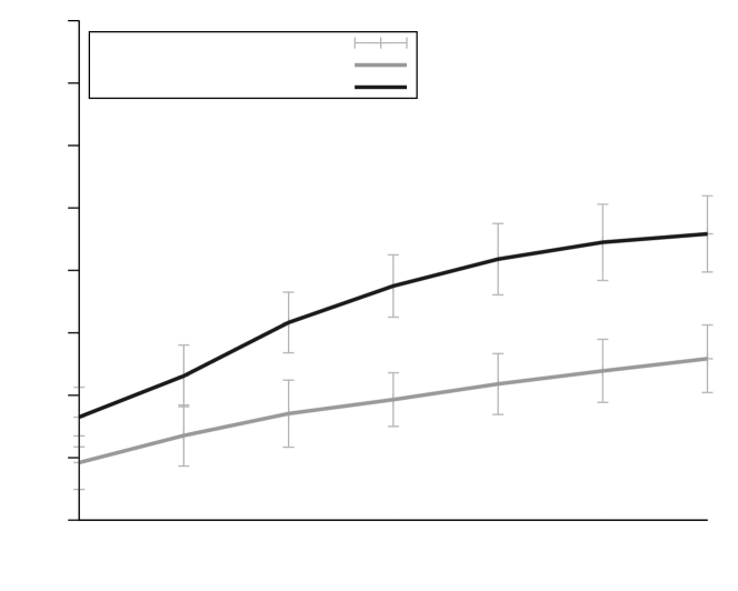
Figure 5: Computing time for the LP solver and the random extraction for a full rank interval matrix of size i×i𝑖𝑖i\times i.

Figure 5 depicts a first experiment showing the average execution time as a function of the dimension of the considered interval matrix for the three methods. The constructed matrices here are square, have a dimension from 2 to 8 and are strictly dominant interval matrices (r=m𝑟𝑚r=m). This experiment shows the exponential increase of the computing time needed while the dimension of the initial matrix for the methods using an LP solver and the apparently better behaviour of the combinatorial method (with a fixed number of iterations).
Refer to caption1e-050.00010.0010.010.112345678

Average computing time (s)

Rank of the initial matrixCriterion on H-matricesCriterion on SDD matricesRandom extraction
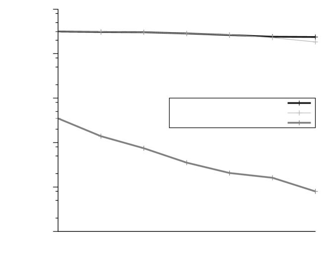
Figure 6: Average computing time (in seconds) over iterations of the LP solver for the search of H-sub-matrices and strictly diagonally dominant sub-matrices, and for the random sub-matrix extraction for an interval matrix of size 8×8888\times 8 as a function of the minimum expected rank.

Figure 6 shows average computing times of the LP solver for the search of H-sub-matrices and strictly diagonally dominant sub-matrices, and for the random sub-matrix extraction for an interval square matrix of dimension 8. In this case the matrix created randomly is constructed with a known minimum rank r𝑟r with 2r82𝑟82\leqslant r\leqslant 8 that is the size of the interval H sub-matrix created. Using the LP solver, the execution time is more or less constant. We stress here the fact that the method using random extraction becomes faster for larger ranks because they are detected very early with Algorithm 4 and because the matrix can contain components equal to 0, the method using H-matrices in the case where u𝑢u is fixed as presented can no longer be applied since a division by 0 can occur in the linear program (21).

Finally two last experiments are provided: they use a different technique to construct the interval matrix. To test the efficiency of the proposed algorithms, matrices with known rank r𝑟r are built. For that purpose, a triangular matrix A𝐴A (with (A)ii0, 1irformulae-sequencesubscript𝐴𝑖𝑖01𝑖𝑟(A)_{ii}\neq 0,\ 1\leqslant i\leqslant r) is first created. It is the upper left part of a matrix Jn×n𝐽superscript𝑛𝑛J\in\mathbb{R}^{n\times n} with nr𝑛𝑟n\geqslant r. The (nr)𝑛𝑟(n-r) remaining columns of J𝐽J are created as linear combinations of the r𝑟r first columns. Then a sequence of rotations are applied to the matrix J𝐽J (here we applied n+1𝑛1n+1 rotations). An angle θisubscript𝜃𝑖\theta_{i} is chosen randomly with 0θiπ0subscript𝜃𝑖𝜋0\leqslant\theta_{i}\leqslant\pi to compose the rotation matrix. A pair (k,l)𝑘𝑙(k,l) with kl𝑘𝑙k\neq l and 1k,lnformulae-sequence1𝑘𝑙𝑛1\leqslant k,l\leqslant n is chosen randomly and the rotation is applied for coordinates (k,l)𝑘𝑙(k,l) and (l,k)𝑙𝑘(l,k). The matrix A𝐴A constructed in this way is not interval.

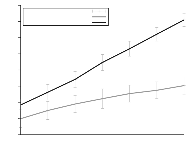
Figure 7 shows the results for a first experiment using this matrix construction which has the advantage to let us know the expected rank of the results. Using Theorem 4.1 as a criteria for sub-matrix extraction generally leads to a sub-matrix of dimension less than the rank of the matrix that is worse than the combinatorial method.
Refer to caption0123456782345678

Estimated rank

Actual rank of the matrixStandard deviationCriterion on SDD matricesRandom extraction
Figure 7: Execution from a matrix J8×8𝐽superscript88J\in\mathbb{R}^{8\times 8} of constant rank i=2,,8𝑖28i=2,\dots,8. Results are average values over 200 computations.

The matrix construction can be used to show the impact of the interval width of the components of the matrix on the method efficiency. For the last experiment, the same matrix construction than the previous one is used except that the components of the matrix constructed are thickened to obtain an interval matrix (the interval [0.25,0.25]0.250.25\left[-0.25,0.25\right] is added to each component of the matrix for one experiment and [0.5,0.5]0.50.5\left[-0.5,0.5\right] for another). Results are shown in Figure 8.
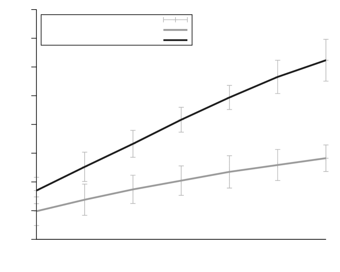
Refer to caption0123456782345678

Estimated rank

Actual rank of the matrix before interval perturbationStandard deviationCriterion on SDD matricesRandom extraction
Refer to caption0123456782345678

Estimated rank

Actual rank of the matrix before interval perturbationStandard deviationCriterion on SDD matricesRandom extraction
Figure 8: Estimate of the rank of an interval matrix 𝐀𝕀8×8𝐀𝕀superscript88{\bf A}\in\mathbb{IR}^{8\times 8} of constant rank i=1,,8𝑖18i=1,\dots,8. Upper picture: [0.25,0.25]0.250.25\left[-0.25,0.25\right] is added to each component, lower picture: [0.5,0.5]0.50.5\left[-0.5,0.5\right] is added to each component Results are average values over 200 evaluations. Standard deviation is provided.

These experiments show that the combinatorial method is better than the method extracting strictly diagonally dominant sub-matrices. This is due to Theorem 4.3 which can detect a bigger subset of regular matrices than just strictly diagonally dominant ones.

Limitations

As previously mentioned, this method cannot guarantee to obtain the sub-matrix of maximum rank. For a given function f:𝒟mn:𝑓𝒟superscript𝑚superscript𝑛f:\mathcal{D}\subseteq\mathbb{R}^{m}\rightarrow\mathbb{R}^{n} of constant rank r𝑟r, only pr𝑝𝑟p\leqslant r components can be detected from the LP program (16). An inner approximation will be obtained only for these p𝑝p components of f𝑓f.

5 Computation of an inner approximation of the range of a vector-valued function

This section shows some results of the computation of inner approximations of immersions and submersions. The functions considered in these examples satisfy (3) with r𝑟r known.

5.1 Immersion

Consider the problem of finding the range of the function

f:2:𝑓superscript2\displaystyle f:\mathbb{R}^{2} 3absentsuperscript3\displaystyle\rightarrow\mathbb{R}^{3}
(u,v)𝑢𝑣\displaystyle(u,v) {f1(u,v)=cos(u)cos(v)f2(u,v)=sin(u)cos(v)f3(u,v)=sin(v)maps-toabsentcasessubscript𝑓1𝑢𝑣𝑢𝑣subscript𝑓2𝑢𝑣𝑢𝑣subscript𝑓3𝑢𝑣𝑣\displaystyle\mapsto\left\{\begin{array}[]{l}f_{1}(u,v)=\cos(u)\cos(v)\\ f_{2}(u,v)=\sin(u)\cos(v)\\ f_{3}(u,v)=\sin(v)\end{array}\right. (25)

over the box (𝐮,𝐯)=([3π2+τ,2πτ];[τ,π2τ]),τ>0formulae-sequence𝐮𝐯3𝜋2𝜏2𝜋𝜏𝜏𝜋2𝜏𝜏0({\bf u},{\bf v})=(\left[\frac{3\pi}{2}+\tau,2\pi-\tau\right];\left[\tau,\frac{\pi}{2}-\tau\right]),\ \tau>0. f𝑓f is of constant rank 2 in (𝐮,𝐯)𝐮𝐯({\bf u},{\bf v}). The rank is equal to the dimension of the domain of f𝑓f, it is then an immersion. Corollary 2 can be used to get an inner approximation of the range of two components of f𝑓f. Here we compute the range of the two first components, but the two last or the first and the last components could also be considered.

Refer to caption-0.200.20.40.60.81-1-0.8-0.6-0.4-0.2000.20.40.60.81
Figure 9: Example 1: Range of the immersion defined in (25) for the initial domain (𝐮,𝐯)=([3π2+τ,2πτ];[τ,π2τ]),τ>0formulae-sequence𝐮𝐯3𝜋2𝜏2𝜋𝜏𝜏𝜋2𝜏𝜏0({\bf u},{\bf v})=(\left[\frac{3\pi}{2}+\tau,2\pi-\tau\right];\left[\tau,\frac{\pi}{2}-\tau\right]),\ \tau>0.

Figure 9 represents the image of (𝐮,𝐯)𝐮𝐯({\bf u},{\bf v}) by f𝑓f which has no volume in its co-domain 3superscript3\mathbb{R}^{3}. Results of the computation of an inner approximation of this range are shown in Figure 5.1 for different values of ε𝜀\varepsilon in Algorithm 1. The smaller the ε𝜀\varepsilon, the more accurate the inner approximation and the longer the computing time. In Figure 5.1, empty boxes in gray represent boxes Algorithm 1 was unable to prove to be in the range. Black boxes all belong to the range.

& Refer to caption-1-0.8-0.6-0.4-0.2000.20.40.60.81 Refer to caption-1-0.8-0.6-0.4-0.2000.20.40.60.81
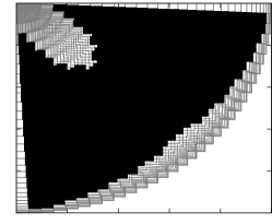
Figure 10: Example 1: Results of the computation of an inner approximation for different values of parameter ε𝜀\varepsilon (0.1, 0.06, and 0.02).

The left part of Figure 5.1 is for ε=0.1𝜀0.1\varepsilon=0.1, the middle part for ε=0.06𝜀0.06\varepsilon=0.06 and the last part for ε=0.02𝜀0.02\varepsilon=0.02. The computing times are respectively 0.026 s, 0.10 s, and 0.64 s.

5.2 Submersion

Consider now the computation of an inner approximation of the range of the function

f:(𝐱,𝐲,𝐳)3:𝑓𝐱𝐲𝐳superscript3\displaystyle f:({\bf x},{\bf y},{\bf z})\subseteq\mathbb{R}^{3} 2absentsuperscript2\displaystyle\rightarrow\mathbb{R}^{2}
(x,y,z)𝑥𝑦𝑧\displaystyle(x,y,z) {(x+rcos(z))cos(y)(x+rsin(z))sin(y)maps-toabsentcases𝑥𝑟𝑧𝑦𝑥𝑟𝑧𝑦\displaystyle\mapsto\left\{\begin{array}[]{l}(x+r\cos(z))\cos(y)\\ (x+r\sin(z))\sin(y)\end{array}\right. (28)

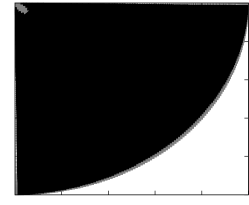
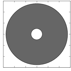
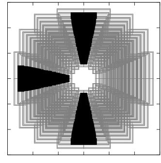
with (𝐱,𝐲,𝐳)=([2,4.5],[0,2πτ],[0,2πτ])𝐱𝐲𝐳24.502𝜋𝜏02𝜋𝜏({\bf x},{\bf y},{\bf z})=(\left[2,4.5\right],\left[0,2\pi-\tau\right],\left[0,2\pi-\tau\right]), τ=103𝜏superscript103\tau=10^{-3}. Figure 11 represents the range of f𝑓f and Figure 5.1 represents different computations of an inner approximation according to the parameter ε𝜀\varepsilon in Algorithm 1. On Figure 5.1a ε=0.5𝜀0.5\varepsilon=0.5 and it took 0.18s to get the result. For Figure 5.1b, ε=0.3𝜀0.3\varepsilon=0.3 and computation time is 6.25s. In Figure 5.1c, it took 145.53s with ε=0.1𝜀0.1\varepsilon=0.1 to get these results. Finally Figure 5.1 d is for ε=0.05𝜀0.05\varepsilon=0.05 and the computing time is 838.67s. The time needed for computation is longer for this experiment than for the previous one on immersion. It is due to the fact that the Jacobian of f𝑓f is not of full rank in the entire domain ([2,4.5],[0,2πτ],[0,2πτ])24.502𝜋𝜏02𝜋𝜏(\left[2,4.5\right],\left[0,2\pi-\tau\right],\left[0,2\pi-\tau\right]). It is why an area (cf. Figure 5.1d remains out of the range of f𝑓f.

Refer to caption-6-4-20246-6-4-20246
Figure 11: Example 2: Range of the submersion defined in (28) for the initial domain (𝐱,𝐲,𝐳)=([2,4.5],[0,2πτ],[0,2πτ])𝐱𝐲𝐳24.502𝜋𝜏02𝜋𝜏({\bf x},{\bf y},{\bf z})=(\left[2,4.5\right],\left[0,2\pi-\tau\right],\left[0,2\pi-\tau\right]), τ=103𝜏superscript103\tau=10^{-3}.

& b) Refer to caption-6-4-20246-6-4-20246 c) Refer to caption-6-4-20246-6-4-20246 d) Refer to caption-6-4-20246-6-4-20246

Figure 12: Example 2: Results of computation of an inner approximation according to the parameter ε𝜀\varepsilon in Algorithm 1 (ε=0.5𝜀0.5\varepsilon=0.5, 0.3, 0.1 and 0.05).

6 Conclusion

Goldsztejn and Jaulin in [5] proposed a way to compute an inner approximation of the range of a vector-valued function. This paper provides an algorithm to evaluate inner approximations of the range of vector-valued functions without restriction on the dimension of its domain and co-domain. Using the proposed algorithm, one is able, for functions from msuperscript𝑚\mathbb{R}^{m} to nsuperscript𝑛\mathbb{R}^{n} to evaluate an inner approximation of the projection of the range of f𝑓f on at most r𝑟r components, where r𝑟r is the rang of the Jacobian matrix of f𝑓f. In the general case, this rank r𝑟r is unknown a priori, it is thus necessary to develop several techniques to extract a sub-matrix of maximal rank from a given interval matrix. The restriction of this method is providing an inner approximation of at most r𝑟r components of the function if this function has a constant rank r𝑟r.

References

  • [1] V.I. Arnold, S.M. Gusein-Zade, and Varchenko A.N. Singularities of differentiable maps, vol. 1. Monographs in Mathematics, 82, 1985.
  • [2] J.P. Aubin and H. Frankowska. Set-valued analysis. Birkhäuser Boston, 2008.
  • [3] P. Cousot and R. Cousot. Abstract interpretation: A unified lattice model for static analysis of programs by construction or approximation of fixpoints. In POPL ’77: Proceedings of the 4th ACM SIGACT-SIGPLAN symposium on Principles of programming languages, pages 238–252. ACM Press, 1977.
  • [4] A. Goldsztejn. A right-preconditioning process for the formal–algebraic approach to inner and outer estimation of ae-solution sets. Reliable Computing, 11(6):443–478, 2005.
  • [5] A. Goldsztejn, L. Jaulin, et al. Inner approximation of the range of vector-valued functions. Reliable Computing, 14:1–23, 2010.
  • [6] G.H. Golub and C.F. Van Loan. Matrix computations, volume 3. Johns Hopkins Univ Pr, 1996.
  • [7] P. Herrero, M.Á. Sainz, J Vehí, and L Jaulin. Quantified set inversion algorithm with applications to control. Reliable Computing, 11(5):369–382, 2005.
  • [8] J.N. Hooker. Integrated methods for optimization, volume 170. Springer, 2011.
  • [9] Y. Ishida and A. Nogi. Reasoning about structure of interval systems: An approach by sign directed-graph. In Proceedings of the 10th International Workshop on Qualitative Reasoning (QR-96), 1996.
  • [10] L. Jaulin, M. Kieffer, Olivier Didrit, and É. Walter. Applied interval analysis: with examples in parameter and state estimation, robust control and robotics. Springer Verlag, 2001.
  • [11] L. Jaulin and É. Walter. Guaranteed tuning, with application to robust control and motion planning. Automatica, 32(8):1217–1221, 1996.
  • [12] E. Kaucher. Interval analysis in the extended interval space IR. Computing Suppl, 2:33–49, 1980.
  • [13] L. Levy. Sur la possibilité de l’équilibre électrique. CR Acad. Sci. Paris, 93:706–708, 1881.
  • [14] A. Makhorin. GLPK (GNU linear programming kit). http://www.gnu.org/software/glpk, 2006.
  • [15] R.E. Moore. Interval analysis, volume 60. Prentice-Hall Englewood Cliffs, New Jersey, 1966.
  • [16] V.M. Nesterov. Interval and twin arithmetics. Reliable Computing, 3(4):369–380, 1997.
  • [17] A. Neumaier. Interval methods for systems of equations, volume 37. Cambridge Univ Pr, 1990.
  • [18] A. Neumaier. Complete search in continuous global optimization and constraint satisfaction. Acta Numerica, 13(1):271–369, 2004.
  • [19] S. Poljak and J. Rohn. Checking robust nonsingularity is np-hard. Mathematics of Control, Signals, and Systems (MCSS), 6(1):1–9, 1993.
  • [20] J. Rohn. Systems of linear interval equations. Linear algebra and its applications, 126:39–78, 1989.
  • [21] J. Rohn. Interval matrices: Singularity and real eigenvalues. SIAM journal on matrix analysis and applications, 14:82–82, 1993.
  • [22] O. Taussky. A recurring theorem on determinants. The American Mathematical Monthly, 56(10):672–676, 1949.
  • [23] L.W. Tu. An introduction to manifolds. Springer, 2010.