Modification of the formation of high-Mach number electrostatic shock-like structures by the ion acoustic instability

Abstract

The formation of unmagnetized electrostatic shock-like structures with a high Mach number is examined with one- and two-dimensional particle-in-cell (PIC) simulations. The structures are generated through the collision of two identical plasma clouds, which consist of equally hot electrons and ions with a mass ratio of 250. The Mach number of the collision speed with respect to the initial ion acoustic speed of the plasma is set to 4.6. This high Mach number delays the formation of such structures by tens of inverse ion plasma frequencies. A pair of stable shock-like structures is observed after this time in the 1D simulation, which gradually evolve into electrostatic shocks. The ion acoustic instability, which can develop in the 2D simulation but not in the 1D one, competes with the nonlinear process that gives rise to these structures. The oblique ion acoustic waves fragment their electric field. The transition layer, across which the bulk of the ions change their speed, widens and their speed change is reduced. Double layer-shock hybrid structures develop.

I Introduction

Collision-less plasma shocks are ubiquitous in the dilute solar system plasmas and in astrophysical plasmas. Their internal structure is fundamentally different from their collisional counterparts, which behave similarly to shocks in gases. Collisional shocks can transform almost instantly the directed flow energy of the incoming upstream plasma into heat by means of binary collisions between the plasma particles. Particle beams are rapidly thermalized and the plasma can be described by a unique temperature value at any position. In the case of collision-less plasma shocks, the upstream plasma is slowed down and heated up by electromagnetic fields as it crosses the shock boundary. Multiple plasma beams can be present at any location and it is possible that a subset of particles is accelerated to high energies by the shock while the bulk of the particles is thermalized. The structure of collision-less shocks depends strongly on the local plasma parameters, in particular on the background magnetic field, on the electron and ion temperatures and on the ion composition. A background magnetic field is particularly important, because it determines the wave mode that mediates the shock.

The key role held by the background magnetic field is evidenced by the Earth’s bow shock, which develops where the solar wind encounters the Earth’s magnetic field. The relative speed between the solar wind and the Earth’s magnetic field exceeds the ion acoustic speed and the Alfvén speed; the boundary separating the solar wind plasma and the magnetosheath’s plasma is thus a shock Sckopke . In spite of its low amplitude of about 5nT SolarWind , the magnetic field of the solar wind assumes a vital role in determining the structure of the bow shock. If the solar wind’s magnetic field is oriented perpendicularly QuasiPerp to the shock’s normal, the shock transition layer is narrow. As the angle between the magnetic field and the shock normal decreases, the shock transition layer widens QuasiPar . The shock boundary changes into a train of SLAMS (short large amplitude magnetic structures) for small angles SLAMS .

The most basic type of shock develops in unmagnetized plasma. Such shocks have been observed in a wide range of experiments, e.g. Exp1 ; Exp2 ; Exp3 ; Exp4 ; Exp5 ; Exp6 , they have been addressed theoretically Bardotti ; Sorasio ; Raadu ; Yannis ; Antoine and by means of numerical particle-in-cell (PIC) and hybrid simulations ForslundA ; ForslundB ; Karimabadi ; Kato ; Parametric . The shock is sustained by the electrostatic field that is tied to the density gradient between the downstream and upstream plasmas. This density gradient results in turn from the slow-down of the upstream ions by the electrostatic field as they cross the shock transition layer. The electric field and the plasma compression are thus conjoined processes. The ambipolar electrostatic field is a consequence of the different electron and ion mobilities. Electrons can escape from the denser downstream plasma into the upstream plasma. A positive net charge develops in the downstream plasma and a negative one in the upstream plasma. The space charge results in an electrostatic field across the shock that helps confining the downstream electrons. A shock forms if this electric field is strong enough to slow down the incoming upstream ions to a speed in the downstream reference frame, which is comparable to the downstream ion’s thermal speed. This condition imposes an upper limit on the speed, or more specifically on the Mach number, of non-relativistic and unmagnetized collision-less shocks.

Here we examine by means of PIC simulations the formation of electrostatic structures out of the collision of two equal and spatially uniform plasma clouds at a contact boundary, which is orthogonal to the collision direction. Each cloud consists of one electron and one ion species. The electrons and ions of each cloud have the same density, the same temperature and the same mean speed at the simulation’s start. The plasma is thus free of net charge and current and initially all electromagnetic field components are set to zero. No particles are introduced after the simulation has started. The Mach number, which corresponds to the collision speed between both clouds, is close to the maximum one, which resulted in the formation of electrostatic shock-like structures in similar simulations Parametric . These shock-like structures can at least initially not be classified GreatPaper as electrostatic shocks due to transient effects, which arise from our choice of initial conditions. The shock-like structures tend to form slowly for high Mach numbers of the collision speed, which allows for the simultaneous development of the ion acoustic instability between counter-streaming ion beams Karimabadi ; Kato ; ForslundC . It has been shown recently that the ion acoustic instability can destabilize an already existing electrostatic shock Kato . Here we examine this instability as it develops already during the formation phase of a shock. Our results are as follows.

Our first simulation study resolves only the direction that is aligned with the relative velocity vector between both clouds. This geometry excludes the ion acoustic instability for the considered initial conditions. The simulation confirms that the formation time of the shock-like structures is delayed by the large collision speed; the electrostatic fields that mediate these structures grow slowly. They need several tens of inverse ion plasma frequencies to reach the amplitude, which is necessary to let the counter-streaming ion beams collapse into a pair of shock-like structures. This delay is comparable to the one observed in Ref. Parametric for a similar collision Mach number and for ions with a charge-to-mass ratio that is 2/3 of the one used here, suggesting that the peak Mach number of such structures may not depend strongly on the value chosen for this ratio. The latter can have a significant impact on the shock formation for faster collisions MassRatio . These shock-like structures gradually evolve into electrostatic shocks as they separate. The forward and reverse shocks are time-stationary in their rest frame in the 1D simulation and they propagate at a constant speed, as in previous one-dimensional PIC simulation studies Parametric .

Our 2D simulation study employs initial conditions that are identical to those of the first one and it has the purpose to assess the impact of the ion acoustic instability, which is observed in the context of laser plasma experiments Bulanov , on the shock formation. This instability develops between two counterstreaming ion beams if their relative speed is significantly less than the thermal speed of the electrons. The ion acoustic waves can only grow if the projection of the beam velocity vector onto the direction of the wave vector yields a sub-sonic speed modulus. This constraint implies for our initial conditions that the waves must move obliquely to the beam velocity vector ForslundC , which requires a 2D simulation geometry. We observe that the electric field of the shock-like structures and the one due to the ion acoustic instability develop simultaneously and eventually reach a comparable amplitude. The ion acoustic waves fragment the shock’s electric field altering the balance between the downstream pressure, which has contributions by ram pressure and thermal pressure, and the pressure of the incoming upstream plasma that sustains the shock-like structure. The velocity change of the bulk of the inflowing ions is comparable to the ion acoustic speed and, thus, well below that observed in the 1D simulation. We observe a widening of the transition layer, across which the ions change their speed as they move from the upstream to the downstream region.

A comparison of the electron velocity distributions downstream of the shocks computed by the 1D and 2D simulations suggests that the flat-top distribution, which is observed in the 1D simulation and in Ref. Parametric , results from the reduced simulation geometry. A pronounced maximum of the velocity distribution function develops at low speeds in the 2D simulation and the distribution function gradually decreases with increasing speed moduli. We attribute the modified velocity distribution function to the interaction of electrons with the strong ion acoustic waves.

The structure of our manuscript is as follows. Section 2 describes qualitatively how an electrostatic shock forms, it summarizes the numerical scheme of a PIC code and it details our initial plasma conditions. Section 3 presents the simulation results and section 4 is the discussion.

II Initial conditions and the simulation method

II.1 The shock model

Non-relativistic electrostatic and unmagnetized shocks form due to the ambipolar electric field of a plasma density gradient and are stabilized by it. Figure 1 illustrates this mechanism assuming that the ions are cool.

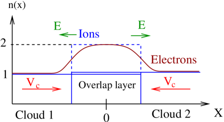
Figure 1: Shock formation: Two equal plasma clouds consisting of electrons and ions, each with the density $n_{0}=1$, collided initially at the position $x=0$ at the speed $2v_{c}$. The figure shows the system a short time after the collision, when clouds 1 and 2 have interpenetrated for a short distance. The ion density in this overlap layer is $n(x)=2$. Some electrons stream out of this layer due to their high mobility and the resulting net charge puts the overlap layer on a positive potential relative to the surrounding plasma clouds.

Two plasma clouds, each consisting of electrons and ions, collide initially at the position $x=0$. The ions and electrons of each cloud move at the equal mean speed modulus $v_{c}$ towards $x=0$. The density of the electrons and of the singly charged ions is $n_{0}$ and each plasma cloud is thus initially free of any net charge and current. The low thermal speed of the ions preserves their number density distribution on electron time scales. The ion number density in the overlap layer is thus initially $2n_{0}$ and it decreases to $n_{0}$ at the two boundaries between the overlap layer and both incoming plasma clouds. Some electrons diffuse across the boundaries, leaving behind a positively charged overlap layer. The overlap layer goes on a positive potential relative to both clouds, which is independent of $v_{c}$. The associated unipolar electric field at each of the boundaries points towards the incoming plasma clouds. It thus confines electrons to the overlap layer, it results in an expansion of ions from the overlap layer and in a slow-down of the ions of the incoming plasma clouds as they cross the overlap layer’s boundary.

The evolution of the overlap layer is determined by how the kinetic energy of the incoming ions in the reference frame of the overlap layer compares to the potential energy they gain as they enter the overlap layer. If the kinetic energy is significantly larger, the ions of both clouds overcome the positive potential of the overlap layer and the counterstreaming ions thermalize via beam instabilities. Otherwise, the evolution of the overlap layer depends on how the pressure of the plasma in the overlap layer compares to the pressure that is excerted on its boundary by the incoming plasma. This balance is mediated by the ambipolar electric field. The overlap layer expands in the form of a rarefaction wave Sack , if its pressure can not be balanced by the pressure of the upstream plasma. A shock solution can exist if the pressure of the overlap layer and of the upstream plasma are equal in some reference frame. The shock is stationary in this frame, which is henceforth denoted as the shock frame. The ram pressure dominates the upstream plasma pressure in this frame and the thermal pressure contributes most to that of the downstream plasma.

The formation of an electrostatic shock is an inherently non-linear process that does not depend on wave and beam instabilities for the low Mach number of the collision speed, which we consider here. This is demonstrated by our 1D simulation, where the ion beam instability is excluded by the simulation geometry while the Buneman instability Buneman ; Amano is suppressed by the large thermal speed of the electrons. The slow-down of the incoming ions in the reference frame of the overlap layer is tied to a density increase via the continuity equation. The ion density in the overlap layer increases beyond $2n_{0}$ and the potential difference between the compressed overlap layer and the incoming plasma cloud increases accordingly. The larger potential difference results in an even stronger slow-down and compression of the incoming ions. This non-linear and self-amplifying process, which has been resolved experimentally Exp6 , is eventually halted by the formation of a shock. The shock separates the downstream region, which is the compressed overlap layer, from the upstream region. The latter corresponds to the incoming unperturbed plasma cloud. The frequently observed partial reflection of the incoming ions by the shock potential ForslundA ; ForslundB gives rise to a foreshock region that is occupied by the incoming plasma cloud and by a beam of shock-reflected ions.

II.2 The particle-in-cell method and the initial conditions

The particle-in-cell (PIC) method approximates the plasma by an ensemble of computational particles (CPs) and the collective electromagnetic fields $\mathbf{E}$ and $\mathbf{B}$ are computed on a numerical grid. These fields are generated by the current- and charge density distributions $\mathbf{j}(\mathbf{x},t)$ and $\rho(\mathbf{x},t)$ in the plasma. The electromagnetic fields are evolved in time by Ampère’s and Faraday’s laws,

$$\nabla\times\mathbf{B}=\mu_{0}\mathbf{j}+\mu_{0}\epsilon_{0}\partial_{t}\mathbf{E},$$ (1)

$$\nabla\times\mathbf{E}=-\partial_{t}\mathbf{B},$$ (2)

which are discretized and represented on a numerical grid. Gauss’ law is either fulfilled as a constraint or through a correction step while $\nabla\cdot\mathbf{B}=0$ is usually preserved to round-off precision.

Each CP is characterized by a charge $q_{j}$ and mass $m_{j}$, by a position vector $\mathbf{x}_{i}$ and by a velocity vector $\mathbf{v}_{i}$. The subscript denotes the $i^{th}$ CP of the ensemble that represents the plasma species $j$. The ratio $q_{j}/m_{j}$ must be equal to that of the approximated plasma species, which can be electrons, positrons or ions. The relativistic momentum $\mathbf{p}_{i}$ of each CPs is evolved in time with a discretized form of the Lorentz force equation $d\mathbf{p}_{i}/dt=q_{j}\left(\mathbf{E}(\mathbf{x}_{i})+\mathbf{v}_{i}\times\mathbf{B}(\mathbf{x}_{i})\right)$. The momentum of the CP is $\mathbf{p}_{i}=m_{j}\Gamma_{i}\mathbf{v}_{i}$ and $\Gamma_{i}$ is its relativistic factor. The position is updated with $\mathbf{v}_{i}$ and the simulation time step. The electromagnetic fields in the Lorentz force equation have been interpolated from the grid to the position of the CP. The charge and current contributions of each CP are interpolated back to the grid. The contributions of all CPs are summed up to give $\rho(\mathbf{x})$ and $\mathbf{j}(\mathbf{x})$, which are used to update the electromagnetic fields on the grid.

The ensemble properties of the CPs are close to those of a true plasma provided that the numerical resolution is adequate. The CPs interact via the collective electromagnetic fields, while binary collisions are usually neglected. PIC codes can represent all kinetic wave modes and processes captured by the Vlasov-Maxwell set of equations Dupree , provided that the numerical resolution is appropriate. An in-depth description of the PIC method can be found elsewhere Dawson . We use here the TwoDem code that is based on the virtual particle-mesh method OldPIC . The code solves the relativistic equations of motion for the CPs. Our initial conditions imply however that all velocities stay non-relativistic.

We perform two simulations, which use the same initial conditions for the plasma. The simulation box with length $L$ is subdivided along the x-direction. Plasma cloud 1 is placed in the interval $-L/2\leq x<0$ and the interval $0<x\leq L/2$ is occupied by the plasma cloud 2. Each cloud is composed of one electron species and one species of singly charged ions. Both have the number density $n_{0}$, which defines the electron plasma frequency $\omega_{pe}={(n_{0}e^{2}/m_{e}\epsilon_{0})}^{1/2}$. The ion-to-electron mass ratio is set to $m_{i}/m_{e}=$ 250, giving an ion plasma frequency $\omega_{pi}=\omega_{pe}/250^{1/2}$. The spatially uniform electrons and ions have a Maxwellian velocity distribution with the temperature 10 eV. The electron thermal speed is $v_{e}=1.325\times 10^{6}$ m/s and that of the ions is $v_{i}=v_{e}/250^{1/2}$. The electrons and ions of each cloud move at the speed $v_{c}=3\times 10^{5}$ m/s towards $x=0$. The low collision speed $2v_{c}/v_{e}\approx 0.45$ suppresses the Buneman instability between the ions of one cloud and the electrons of the second cloud.

We define the ion acoustic speed $v_{s}$ through $v_{s}^{2}=\gamma_{s}k_{B}(T_{e}+T_{i})/m_{i}$. This speed is meaningful in a fluid model, where collisions enforce a single Maxwellian velocity distribution and, thus, a single temperature for electrons and for each ion species at any given position and where Landau damping is absent. The ion acoustic waves are Landau damped in a kinetic collision-less framework unless the electrons are much hotter than the ions. Multiple beams of particles of a single species can be present at the same location and the velocity distribution is not necessarily a Maxwellian one. The ion acoustic speed and the shock’s Mach number are thus not as meaningful in a collision-less plasma as they are in a fluid model. We introduce the ion acoustic speed here to compare our initial conditions, which involve Maxwellian velocity distributions for one electron and one ion species at each point in space, to those in related simulation studies and to the conditions found in laser-generated or astrophysical plasma. We assume that both species have the same adiabatic constant $\gamma_{s}=5/3$, which gives us the Mach number of the collision speed $v_{c}/v_{s}\approx 2.3$.

The 1D simulation resolves the x-direction by 3000 simulation grid cells of size $\Delta_{x}=0.95\lambda_{D}$, where the Debye length $\lambda_{D}=v_{e}/\omega_{pe}$. Electrons and ions are each represented by 4464 CPs per cell. The 1D simulation resolves a time interval $t\omega_{pi}=157$. The 2D simulation employs 2500 grid cells along the x-direction and 300 grid cells along the y-direction. The cell size $\Delta_{x}=\Delta_{y}=0.95\lambda_{D}$. Electrons and ions are each represented by 160 CPs per cell. We employ periodic boundary conditions and we do not introduce new particles after the simulations have started. The two colliding electron-ion clouds are thus the only plasma constituents throughout the simulation. The back ends of the plasma clouds detach from the boundaries in the x-direction and move towards the center of the box. The 2D simulation covers a time interval $t\omega_{pi}=86$ and in this simulation $tv_{c}\approx L/8$. The simulations are thus stopped long before the front of one plasma cloud reaches the back end of the counter-streaming second plasma cloud.

III The simulation results

In what follows we present the results of our 1D and 2D simulations. The electric field amplitude is expressed in units of $\omega_{pe}m_{e}c/e$, space in units of the electron Debye length $\lambda_{D}$ and time in units of $\omega_{pi}^{-1}$.

III.1 The 1D simulation

Figure 2 shows the spatio-temporal evolution of the electric field in the 1D simulation, which can be subdivided into three intervals. The first interval $t\omega_{pi}<5$ corresponds to a shock-less interpenetration of both plasma clouds, as depicted in Fig. 1. Strong electric fields are observed in the spatial interval $-5<x/\lambda_{D}<5$ during this time. The ion density gradient at both boundaries of the overlap layer is large, resulting in a strong ambipolar electrostatic field. The ion density gradient is eroded in time due to ion diffusion, which is a consequence of the ion’s thermal velocity spread. The electric field amplitude decreases accordingly and it spreads out in space. The potential difference between the overlap layer and the incoming plasma clouds remains unchanged though, because it is determined by the difference in the positive charge density $\approx en_{0}$ between the overlap layer and the incoming plasma cloud and by the electron temperature.

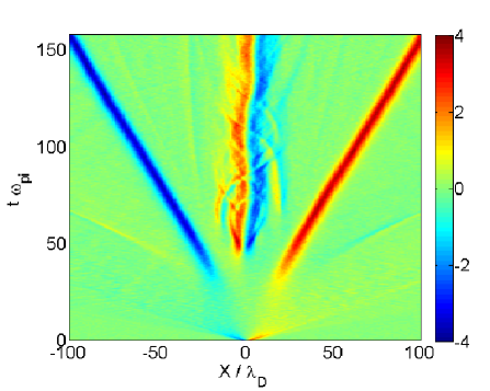
Figure 2: The spatio-temporal electric field distribution in the 1D simulation: The color corresponds to $10^{3}E_{x}$, space is given in units of the electron Debye length $\lambda_{D}$ and time is normalized to the ion plasma frequency $\omega_{pi}$.

The second time interval between $5<t\omega_{pi}<30$ is characterized by a broad distribution of weak electric fields that seem to maintain a constant amplitude. The positive potential of the overlap layer is not capable of slowing down the ions of both incoming plasma clouds to a speed in the rest frame of the overlap layer that is comparable to the ion thermal speed; no shock develops. A lower value of $v_{c}$ would result in their formation on electron time scales. However, the potential of the overlap layer in the 1D simulation slows down and compresses the incoming ions close to the boundary and the ion density is increased locally beyond $2n_{0}$. The positive potential within the overlap layer and, thus, the ion compression increase. The ion accumulation takes place at the boundary between the overlap layer and the incoming plasma cloud if the ions are cold. The thermal diffusion of warm ions implies though that this boundary spreads out. The ion compression beyond the density $2n_{0}$ is achieved in this case at the location, which corresponds to the maximum of the electrostatic potential.

The coupling between the ion slow-down and the increase of the electrostatic potential implies that this is a self-amplifying process. In what follows we refer to this instability as the ion compression instability. Eventually the potential difference between the compressed overlap layer and the incoming plasma is large enough to let both ion density accumulations collapse into shock-like structures during the time $40<t\omega_{pi}<50$.

We observe two electric field pulses in the third time interval $t\omega_{pi}>50$, which are propagating away from $x=0$ at a constant speed. Their propagation speed in the reference frame of the simulation box can be estimated from Fig. 2 to be $|v_{p}|\approx 80\lambda_{D}/(110\omega_{pi}^{-1})$ or $|v_{p}|/v_{s}\approx 0.3$. Their Mach number in the reference frame of the incoming plasma cloud and camputed with respect to the initial ion acoustic speed is $M_{s}\approx 2.6$, since $v_{c}/v_{s}\approx 2.3$. This Mach number and the formation time are similar to the ones of the fastest collision in Ref. Parametric , which resulted in shocks. The electric field demarcates the transition layer of the shock-like structure, which has here a width of about 10 $\lambda_{D}$. A bipolar electric field structure is present at $x\approx 0$. The polarization of this field distribution implies that a negative excess charge is present at $x\approx 0$, which is typical for an ion phase space hole IonHole .

We compute the potential $U(k\Delta_{x})$ at the cell $k$ from the electric field distribution (Fig. 2) through the integration $U(k\Delta_{x})=-\sum_{i=1}^{k}E_{x}(i\Delta_{x})\,\Delta_{x}$, where all quantities are given here in their unnormalized SI units. The cell with the index $i=1$ corresponds to the left boundary. We express the potential $U$ in units of $E_{k}/e$ with $E_{k}=m_{i}{(2.6v_{c}/2.3)}^{2}/2$. This is the kinetic energy of an ion in the reference frame of the electric pulse, which moves towards the pulse at the speed $v_{c}$ in the box frame. The mean value of the fully developed potential is subtracted. The potential $\tilde{U}$ in this normalization is shown in Fig. 3.

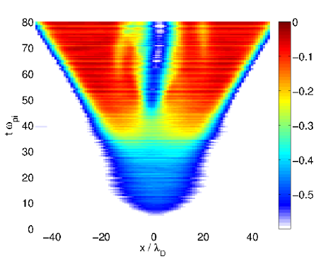
Figure 3: The normalized electrostatic potential $\tilde{U}(x)$.

It grows first at $x\approx 0$ and reaches a pratically stationary distribution between $10<t\omega_{pi}<30$. It grows to larger values at $t\omega_{pi}\approx 40$ and at $|x|/\lambda_{D}\approx 20$. This is well behind the positions $|x|/\lambda_{D}=40v_{c}/(\omega_{pi}\lambda_{D})\approx 150$ that would be reached by ions with the speed modulus $v_{c}$ that moved away from the position $x=0$ at $t=0$. The potential depletion at $x\approx 0$ forms together with the pair of electric field pulses.

Figure 4 shows the plasma phase space distribution at the time $t\omega_{pi}=86$ when the pair of electric field pulses and the potential depletion at $x\approx 0$ have fully developed (See Fig. 3). The online enhancement of Fig. 4 animates the time evolution of the phase space density for $0\leq t\omega_{pi}\leq 157$. It visualizes the ion compression instability at the simulation’s start, which is characterized by a gradual slow-down of the ions in the overlap layer. We focus in Fig. 4 and in its online enhancement on the interval around the (forward) shock-like structure that moves towards increasing values of $x$.

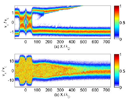
Figure 4: The phase space distributions $f_{i,e}(x,v_{x})$ from the 1D simulation at the time $t\omega_{pi}=86$: Panel (a) shows the ion distribution and panel (b) shows the electron distribution. Space and velocity are expressed in units of the Debye length $\lambda_{D}$ and of the initial cloud speed $v_{c}$. The density is normalized to its peak value and displayed on a linear color scale (enhanced online).

Figure 4(a) reveals the presence of shock-like structures at the positions $|x|/\lambda_{D}\approx 50$, which coincide with those of the strong unipolar electrostatic fields in Fig. 2. A single ion population with a non-Maxwellian velocity distribution is observed in most of the downstream region between both shock-like structures. The only exception is the ion phase space hole, which is located at $x\approx 0$ and gives rise to the bipolar electric field in Fig. 2.

The ion beam at $x/\lambda_{D}>50$ and $v_{x}>0$ shows two distinct phase space distributions. The phase space distribution in the interval $150<x/\lambda_{d}<500$ is that of the ion beam that crossed the overlap layer before the shock-like structures formed. The phase space profile of this beam section is that of a rarefaction wave SarriPRL , which moves relative to the simulation frame of reference. The ions in the phase space interval $50<x/\lambda_{d}<150$ and $v_{c}>0$ consist of two ion populations, which can be seen most easily from the online enhancement of Fig. 4. The source of the faster ions is the downstream plasma. These ions have been accelerated in the upstream direction by the electric pulse. The slower ions with $v_{x}\approx v_{c}$ originate from the incoming plasma cloud. They have been reflected by the shock-like structure. An incoming ion with $v_{x}=-0.5v_{c}$ at $x/\lambda_{D}\approx 60$, which is reflected specularly by a shock that moves in the simulation frame at the speed $v_{p}\approx 0.3v_{c}$ (See Fig. 2), moves back upstream at the speed $v_{x}/v_{c}\approx 1.1$.

The fact that the ions of this beam arise from the upstream population and the downstream population implies that the structure at $x/\lambda_{D}\approx 50$ is not a pure electrostatic shock in the definition of Ref. GreatPaper . An electrostatic shock is composed at best of two distinct ion populations; one population of trapped ions and one population of free ions, which move both from the low potential side ($x/\lambda_{D}>50$ in Fig. 4(a)) to the high potential side. The free ions of the shock-like structure at $x/\lambda_{D}\approx 50$ correspond to the beam of incoming ions with $v_{x}<0$. The ions are slowed down as they cross the structure. The incoming ions, which have been reflected by the shock-like structure, form the trapped population. However, we also find a second population of free ions: those that cross the structure at $x/\lambda_{D}=50$ and move to increasing values of $x$. Ions that flow from the high-potential side to the low-potential side indicate a double layer. According to the classification in Ref. GreatPaper , the structure at $x/\lambda_{D}\approx 50$ and, by symmetry, the one at $x/\lambda_{D}\approx-50$ are hybrid structures. Hence we refer to them as shock-like structures.

The double layer component of the shock-like structure at $x/\lambda_{D}\approx 50$ is strong in Fig. 4(a) because a dense population of ions, which correspond to the free ions that move from the left ($v_{x}>0$) towards the shock-like structure at $x/\lambda_{D}\approx-50$ and traverse the downstream region, reaches the right-moving structure. This is a transient effect. Once the downstream region between both structures is sufficiently wide to thermalize the downstream ions, the ion velocity distribution enclosed by both shock-like structures will change into a Maxwellian one centered at $v_{x}=0$. The number density of the ions, which are fast enough to reach both shock-like structures and feed the double layer, will be much lower. The hybrid structure will change into an electrostatic shock.

Figure 4(b) displays the electron distribution at $t\omega_{pi}=86$. We can subdivide this distribution into three spatial intervals. The electron distribution close to $|x|/\lambda_{D}\approx 700$ corresponds to the initial distribution. The velocity distribution is close to a Maxwellian with a maximum that is shifted by $-v_{c}$. A large circular structure is observed in the displayed interval $x/\lambda_{D}<400$. The increased positive potential, which results from the ion accumulation in this interval, confines the electrons. The trapped electrons move on closed phase space orbits. This trapped electron population is a pre-requisite for double layers and shocks GreatPaper . The velocity distribution within this phase space structure is not Maxwellian but has a phase space density that is constant apart from statistical noise.

The small circular phase space intervals with a reduced electron density in this large cloud of trapped electrons are electron phase space holes. They are stable electrostatic structures in a 1D geometry BGK ; Morse and the online enhancement of Fig. 4 demonstrates their longevity and their stability even when they cross the shock-like structures. The electron distribution in the intervals $400<|x|/\lambda_{D}<500$ just outside of this trapped electron population shows a spatial variation. This variation is caused by the free electrons that escape upstream. The current of the escaping electrons must be compensated by a return current of the incoming electrons, which gives rise to a change of the electron’s mean speed along the x-direction. The incoming upstream electrons are accelerated towards the shock.

A third interval $|x|/\lambda_{D}<50$ in Fig. 4(b) coincides with the downstream region that is enclosed by both shock-like structures. The ion density in this interval exceeds $2n_{0}$ and additional electrons can be confined. The trapped electrons gain kinetic energy as they move into a region with a higher positive potential, which explains why their peak velocity is correlated to the ion density. The peak velocity is not reached by the electrons at $x\approx 0$ due to the negative potential of the ion phase space hole that is located at this position. The fastest electrons are found instead close to the shock-like structures at $|x|/\lambda_{D}\approx 50$ where the potential peaks in Fig. 3.

Figure 5 shows the phase space distributions of the ions and electrons at $t\omega_{pi}=157$. The strong electrostatic fields in Fig. 2 maintain the narrow transition layers in Fig. 5(a), which separate the downstream region with $|x|/\lambda_{D}<100$ from the foreshock regions of both shock-like structures. The ion beams at $x/\lambda_{D}>100$ and $v_{x}\approx v_{c}$ and at $x/\lambda_{D}<-100$ and $v_{x}\approx-v_{c}$ in the displayed spatial interval consist now almost exclusively of ions that were reflected by the shock or accelerated upstream from the downstream region. The ion phase space density distribution in Fig. 5(a) does still not reach its peak value at $v_{x}=0$ in the downstream region, which we would expect from a fully thermalized ion distribution. This aspect has been observed in previous simulations Parametric that employed a different PIC simulation code and an ion-to-electron mass ratio of 400 rather than 250.

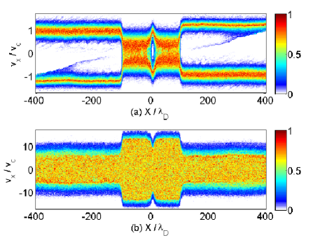
Figure 5: The phase space distributions $f_{i,e}(x,v_{x})$ from the 1D simulation at the time $t\omega_{pi}=157$: Panel (a) shows the ion distribution. Panel (b) shows the electron distribution. Space and velocity are expressed in units of the Debye length $\lambda_{D}$ and of the initial cloud speed $v_{c}$. The density is normalized to its peak value and displayed on a linear color scale.

The electron distribution in Fig. 5(b) does again not show a Maxwellian velocity distribution in the displayed interval. The phase space distribution shows a constant density at low speeds and a fast decrease for $|v_{x}/v_{c}|>7$ in both foreshock regions and for $|v_{x}/v_{c}|>17$ in the downstream region. The potential of the ion phase space hole, which is negative relative to that of the surrounding downstream region, continues to repel electrons, by which it decreases their peak speed at $x\approx 0$. The flat-top velocity distribution of the electrons converges to its initial Maxwellian distribution outside of the foreshock region. The similarity between the plasma distributions in Fig. 4 and 5 evidences that the shock-like structures are stationary in their rest frames in the considered case.

The 1D simulation demonstrates that the selected initial conditions result in the growth and stable propagation of a pair of shock-like structures. However, the positive potential of the overlap layer is initially not sufficiently strong to reflect the incoming ions. The extra potential, which is needed for the shock formation, is provided by a gradual localized accumulation of ions during $t\omega_{pi}\approx 20$. This time delay has important consequences for the shock formation in more than one dimension, which is demonstrated by a direct comparison of the field distributions computed by the 1D and 2D simulations.

III.2 The 2D simulation

Figure 6 visualizes the square root of the energy density $\langle E_{2D}^{2}(x)\rangle_{y}=\frac{1}{300}\sum_{j=1}^{300}\left(E_{x}^{2}(x,j\Delta_{y})+E_{y}^{2}(x,j\Delta_{y})\right)$ of the in-plane electric field, which has been averaged along the y-direction.

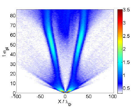
Figure 6: The evolution of $10^{3}{\langle E_{2D}^{2}\rangle_{y}}^{1/2}$, where $\langle E_{2D}^{2}\rangle_{y}$ is the energy density of the in-plane electric field, which has been averaged along the y-direction. Space is normalized to the electron Debye length $\lambda_{D}$ and time is normalized to the ion plasma frequency $\omega_{pi}$. The color scale is linear.

The field distribution evolves qualitatively similarly in the 2D simulation and in the 1D simulation (See Fig. 2) until $t\omega_{pi}\approx 5$. The ion density is gradually increased beyond $2n_{0}$ in both simulations during $5<t\omega_{pi}<15$, but the ion compression instability has not yet resulted in strong electrostatic fields.

The ion compression instability results in a visible field growth after $t\omega_{pi}\approx 25$ in both simulations. The unipolar electric fields, which sustain both shocks in the 1D simulation, saturate at around $t\omega_{pi}\approx 50$ in Fig. 2 and maintain thereafter a constant peak amplitude. The energy density of the in-plane electric field in Fig. 6 evolves qualitatively different after the time $t\omega_{pi}\approx 50$ when it reaches its maximum. The energy density of both pulses decreases and they slow down. The weakening of both pulses is accompanied by a rise of the field energy density in the interval they enclose.

The in-plane components of the electric field at the time $t\omega_{pi}=50$ are shown in Fig. 7.

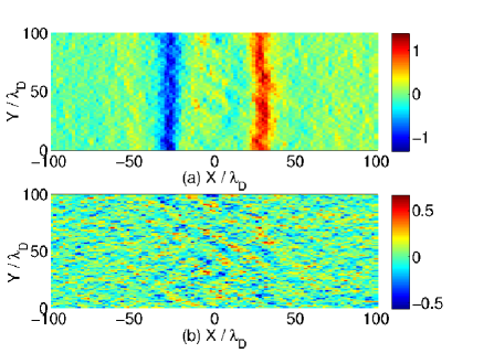
Figure 7: The in-plane electric field at the time $t\omega_{pi}=50$: The upper panel (a) shows $10^{3}E_{x}(x,y)$ and the lower panel (b) shows $10^{3}E_{y}(x,y)$.

The $E_{x}$-component reveals unipolar electric field pulses at $|x|/\lambda_{D}\approx 30$ with a polarity that is typical for the ambipolar electric field. These field pulses put the interval $|x|/\lambda_{D}<20$ on a positive potential relative to the surrounding plasma, which helps confining the electrons. Weak coherent electric field patches are visible within $|x|/\lambda_{D}<30$ in the otherwise noisy $E_{y}$-component. The field distribution is practically planar at this time and the plasma dynamics should be analogeous to that in the 1D simulation.

The electric field topology has changed significantly at the time $t\omega_{pi}=86$, which is evidenced by Fig. 8.

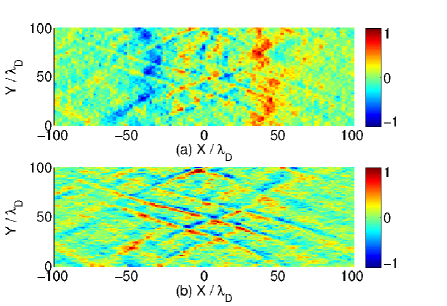
Figure 8: The in-plane electric field at the time $t\omega_{pi}=86$: The upper panel (a) shows $10^{3}E_{x}(x,y)$ and the lower panel (b) shows $10^{3}E_{y}(x,y)$.

The amplitude of $E_{x}$ is only slightly lower than that in Fig. 7. The main difference compared to Fig. 7(a) is that the field distribution is no longer planar. Averaging the electric field energy density at $t\omega_{pi}=86$ like in Fig. 6 results in a broader spatial interval with a lower energy density compared to that at $t\omega_{pi}=50$. The interval enclosed by both pulses shows oblique wave structures. The electric field is no longer planar and anti-parallel to the velocity vector of the incoming ions. The ions are thus not only slowed down along $x$, but they are also deflected along $y$ by the ambipolar electric field. This deflection changes the balance between the upstream pressure and the pressure of the plasma within the overlap layer, which is essential for a shock formation and stabilization.

Figure 9 depicts the electrostatic potentials close to $x=0$ of the field distributions at $t\omega_{pi}=50$ and $86$.

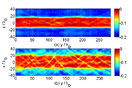
Figure 9: The normalized electrostatic potential $\tilde{U}(x,y)$ computed by the 2D simulation at the time $t\omega_{pi}=50$ (a) and at $t\omega_{pi}=86$ (b). The color scale is linear.

This potential $\tilde{U}(x,y)$ is computed in the same way and with the same normalization as the one shown in Fig. 3. The magnitude of the potential difference between $x\approx 0$ and $|x|/\lambda_{D}\approx 40$ is about 0.2 in both cases. The potential difference that sustains the stable shock-like structures in the 1D simulation is 3-4 times larger and we expect clear differences between the plasma distributions in both simulations. The potential structure at $t\omega_{pi}=50$ is practically planar. It is more diffuse at $t\omega_{pi}=86$ and we observe oblique structures within the high potential region.

We examine the projection of the phase space density distributions of electrons and ions onto the $(x,v_{x})$ plane in form of an animation and at selected time steps. The phase space distributions of electrons and ions are integrated over the y-direction. The purpose of examining the phase space density distributions is to better understand the time-evolution of the ion compression instability and the conditions, under which the ion acoustic instability can grow. The integrated phase space density distributions will also reveal differences caused by the dissimilar electrostatic potentials in the 1D and 2D simulations. We discuss the plasma phase space distribution at $t\omega_{pi}=10$ when the overlap layer has developed while $E_{x}$ is still weak in Fig. 6, at $t\omega_{pi}=50$ when the electric fields driven by the ion compression instability reach their peak amplitude and at $t\omega_{pi}=86$.

The ion phase space distribution in Fig. 10(a) shows some modifications, which were not captured by our simple model of the overlap layer depicted in Fig. 1. The ions of both clouds have interpenetrated in the interval $-55<x/\lambda_{D}<55$. Their mean velocity modulus has decreased below $v_{c}$ at $x\approx 0$, where it has its minimum. Consider the ion beam located in the left half of the simulation box, which moves at a positive speed to the right. As these ions approach the overlap layer, they experience its repelling electrostatic potential. They are accelerated again by the electric field in the interval $x>0$. Some of the ions at the front $x/\lambda_{D}\approx 55$ and $v\approx 1.7v_{c}$ have reached a speed that is higher than that of any ion in the initial distribution. These ions entered the overlap layer before the ambipolar electric field could build up and, hence, they were not slowed down by it. By the time they leave the overlap layer the electric field has developed and the ions are accelerated. This acceleration is strongest at early times (See online enhancement of Fig. 10, which animates the phase space evolution for $0\leq t\omega_{pe}\leq 86$), when the ion density gradient and, thus, the ambipolar electric field are large. They have gained kinetic energy at the expense of electron energy in the time-dependent potential of the overlap layer.

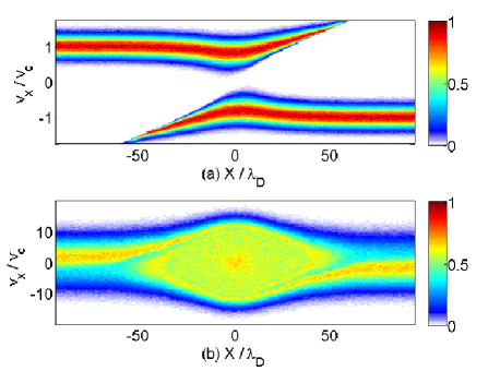
Figure 10: The y-integrated plasma phase space distributions $f_{i,e}(x,v_{x})$ at the time $t\omega_{pi}=10$: Panel (a) shows the ion distribution and panel (b) the electron distribution. Space and velocity are normalized to the electron Debye length $\lambda_{D}$ and the cloud speed $v_{c}$. The density is normalized to the peak value reached in the simulation and the color scale is linear (enhanced online).

The ion beam fronts are no longer parallel to the $v_{x}$ direction. The faster the ions the farther they have propagated during the time interval $t\omega_{p}=10$. The shear of the ion beam front is thus caused by the velocity spread of the ions, which corresponds to diffusion. This diffusion decreases the magnitude of the ion density gradient between the overlap layer and the incoming plasma and thus the amplitude of the ambipolar electric field. Diffusion is responsible for the observed rapid decrease of the electric field amplitude at early times in Fig. 6.

The electron distribution in the online enhancement of Fig. 10(b) shows initially a spiral close to $x=0$ that is brought about by electron trapping in the growing potential of the expanding overlap layer. The electrons would form a vortex in a stationary positive potential. The spiral forms because firstly the entry points of the electrons into the overlap layer move in time to larger values of $|x|$ and, secondly, because the potential difference between the overlap layer and the surrounding plasma increases in time. Electrons that enter the overlap layer at a later time thus get accelerated to a larger speed. The increase of the potential is, in turn, a consequence of the ion compression due to their decreasing mean speed in Fig. 10(a).

Like in the 1D simulation, the current due to the electrons that leave the overlap layer drives an electric field just outside of the overlap layer. The electrons at $x/\lambda_{D}\approx-50$ are accelerated to positive $v_{x}$ by this electric field and they are thus dragged towards the overlap layer. More electrons flow towards the overlap layer than away from it. The net flux of electrons into the overlap layer is a consequence of its expansion in time, which implies that its overall ion number increases. The fastest electrons do not follow the shape of the trapped electron structure. Electrons entering at $x/\lambda_{D}=-95$ with $v_{x}=10v_{c}$ in Fig. 10(b) are accelerated by the positive potential of the overlap layer as they approach $x=0$ and they are decelerated again as they move to larger positive $x$. These electrons are free.

Figure 11 shows the plasma phase space distribution at the time $t\omega_{pi}=50$. The overlap layer has expanded from $|x|/\lambda_{D}=55$ to the position $|x|/\lambda_{D}\approx 300$, which is outside of the displayed interval. A direct comparison of the Figs. 10(a) and 11(a) shows one difference between the ion distributions. Both ion beams are slowed down at the same position $x\approx 0$ at $t\omega_{pi}=10$. They are decelerated most at $x/\lambda_{D}\approx\pm 30$ at $t\omega_{pi}=50$. Both points of maximum ion slow-down and compression are separated in space and enclose a region of enhanced ion density. The electrostatic fields, which are responsible for the ion slow-down at $|x|/\lambda_{D}\approx 30$, are sufficiently strong to reflect a fraction of the incoming ions at these locations. This can be seen more clearly in the animation (online enhancement of Fig. 10).

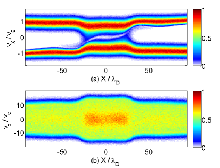
Figure 11: The y-integrated plasma phase space distributions $f_{i,e}(x,v_{x})$ at the time $t\omega_{pi}=50$: Panel (a) shows the ion distribution and panel (b) the electron distribution. Space and velocity are normalized to the electron Debye length $\lambda_{D}$ and the cloud speed $v_{c}$. The density is normalized to the peak value reached in the simulation and the color scale is linear.

The phase space distribution of the electrons in Fig. 11(b) is determined by the electrostatic potential set by the ion density, which is compressed beyond the value $2n_{0}$ in the interval $-30<x/\lambda_{D}<30$. One feature of the electron distribution that sets it apart from its counterpart in the 1D simulation (See Figs. 4(b) and 5(b)) is that it is not a flat top distribution at low speeds. A weak enhancement of the phase space density can be observed at $v_{x}\approx 0$ in the interval $-25<x/\lambda_{D}<25$. The online enhancement of Fig. 10 shows that the electron’s phase space density in this interval continues to grow after $t\omega_{pi}\approx 50$. It is thus temporally correlated with the rise of the energy density close to $x\approx 0$ in Fig. 6.

Figure 12 depicts the plasma phase space distributions at $t\omega_{pi}=86$.

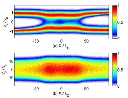
Figure 12: The y-integrated plasma phase space distributions $f_{i,e}(x,v_{x})$ at the time $t\omega_{pi}=86$: Panel (a) shows the ion distribution and panel (b) the electron distribution. Space and velocity are normalized to the electron Debye length $\lambda_{D}$ and the cloud speed $v_{c}$. The density is normalized to the peak value reached in the simulation and the color scale is linear.

The large scale distribution of the ions in the 2D simulation resembles that in the 1D simulation in Fig. 4(a) (not shown) except in the interval displayed in Fig. 12(a). We observe an overlap layer with two dense counter-streaming ion beams and a dilute ion population with $|v_{x}|\approx 0$. The online enhancement of Fig. 10 shows that the velocity gap between both dense ion beams increases again after $t\omega_{pi}\approx 50$, while both ion beams converged along the $v_{x}$-direction in the 1D simulation. The plasma has thus evolved to a different nonlinear state at this time in the 1D and 2D simulations. The counter-streaming ion beams in the 2D simulation are affected significantly less by the positive potential of the overlap layer than those in the 1D simulation, which is a consequence of the different magnitude of the potential. Most ions in the 2D simulation experience the overlap layer as a localized potential maximum, which is not strong enough to slow them down to the ion’s thermal speed in the downstream reference frame. The velocity change of the bulk ions close to $|x|/\lambda_{D}\approx 50$ is of the order of $v_{c}/3$, which is comparable to or below the sound speed $c_{s}$.

An ion distribution, which is symmetric around $v_{x}=0$, corresponds to a hybrid structure with equally strong electrostatic shock and double layer components. The ion distribution in Fig. 4(a) is less symmetric than that in Fig. 12(a). The ion beam in the interval $50<x/\lambda_{D}<100$ and $v_{x}>0$ in Fig. 4(a), which is composed of trapped incoming ions and of ions that are accelerated from the downstream region into the upstream direction, is significantly thinner than the incoming free ion population with $v_{x}<0$. The hybrid distribution in the 1D simulation thus has a much stronger electrostatic shock character than its counterpart in Fig. 12(a) at this time.

The phase space distribution of the electrons in Fig. 12(b) shows a pronounced maximum at $v_{x}\approx 0$ in the interval $-50\leq x/\lambda_{D}\leq 50$. It is closer to a Maxwellian than to a flat-top velocity distribution. We attribute the differences between the electron distributions in Fig. 4(b) and 12(b) to the higher-dimensional phase space dynamics in the 2D simulation. The electron dynamics is confined to the $(x,v_{x})$ plane in the 1D simulation. The oblique electric fields observed in Fig. 8 introduce an electric force component in the y-direction that is a function of both spatial coordinates. The phase space dynamics of the electrons involves in this case the four coordinates $(x,y,v_{x},v_{y})$. The growing amplitudes of the ion acoustic waves (Compare Figs. 7 and 8) imply that they can interact nonlinearly with electrons in a velocity interval that increases in time.

This discrepancy between the electron phase space distributions in the 1D and 2D simulations reveals another reason for why the Mach number is not as meaningful in a kinetic collision-less framework as it is in a collisional fluid theory. The adiabatic index $\gamma_{s}$ is tied to the degrees of freedom in the medium under consideration. The particles of the mono-ionic plasma in the PIC simulation have three degrees of freedom. However, only one degree of freedom is accessible to particles in a 1D simulation of electrostatic processes or in the 2D simulation, if the electrostatic fields are perfectly planar. The onset of the ion acoustic instability makes accessible a second degree of freedom to the plasma and $\gamma_{s}$ can change.

The ion density distributions $n(x)=\int_{-\infty}^{\infty}f_{i}(x,v_{x})dv_{x}$ computed from the y-integrated phase space distributions Fig. 4(a) and Fig. 12(a) shed further light on the different plasma state in the 1D and 2D simulations. Figure 13 compares both distributions at $t\omega_{pi}=86$.

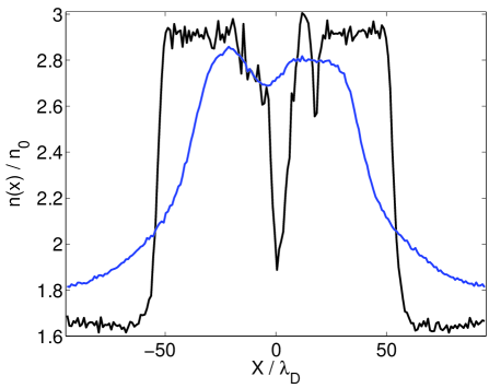
Figure 13: The y-integrated ion density distributions in the 1D simulation (black curve) and in the 2D simulation (blue curve) at $t\omega_{pi}=86$.

The ion density distribution in the 1D simulation shows steep gradients between the downstream region and the foreshock regions of both shock-like structures. The ion density grows from the foreshock value $n(x)\approx 1.65n_{0}$ close to $|x|/\lambda_{D}\approx 60$ to the downstream value $n(x)\approx 2.9$ over $10\lambda_{D}$. The ion cavity at $x\approx 0$ is caused by the ion phase space hole. The ion density gradient in the 2D simulation is lower and the peak density is reached at $|x|/\lambda_{D}\approx 20$, which is well behind the shock location in the 1D simulation. The wide transition layer in the 2D simulation is partially a consequence of averaging the ion density over the y-direction; the potential distribution in Fig. 9 demonstrates that the overlap layer is not perfectly planar at this time. Another important reason for the wide transition layer is that the ion beams in Fig. 12(a) are slowed down less and over a wider spatial interval than the ion beams in Fig. 4(a), which results according to the continuity equation in a lower density gradient.

We have observed significant differences in the plasma evolution in the 1D and 2D simulations during the time interval $50\leq t\omega_{pi}\leq 86$ (Compare Figs. 2 and 6). We have attributed these difference to the oblique electrostatic structures in Fig. 9 that are geometrically suppressed in the 1D simulation. Their obliquity suggests that they are driven by an ion acoustic wave instability between the two ion beams, which counter-stream at a speed that exceeds the ion acoustic speed ForslundC . Their growth time is of the order of ten inverse ion plasma frequencies, which suggests that the instability is ionic.

We turn towards the ion density distribution in the 2D simulation as a means to determine whether or not the ion acoustic instability is involved and if it is indeed responsible for the different ion evolution in both simulations. The ion acoustic instability is purely growing (the wave frequency has no real part) for our symmetric beam configuration ForslundC . Its phase speed vanishes. We thus expect the growth of spatially stationary oblique ion density modulations in the overlap layer. The presence of such structures is confirmed by Fig. 14, which shows the ion density distribution at $t\omega_{pi}=72$

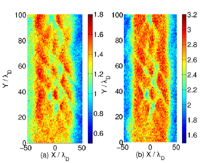
Figure 14: The ion density distributions in a section of the 2D simulation box at the time $t\omega_{pi}=72$. Panel (a) shows the distribution of the ion beam that moves to increasing values of $x$. Panel (b) shows the total ion density (enhanced online).

(The online enhancement of Fig. 14 animates the ion density evolution until $t\omega_{pi}=72$). The ion distribution is initially planar. The online enhancement shows the formation of the overlap layer (See Fig. 10), which is followed by a compression phase that results in a planar ion pile-up. The density of the left ion beam (panel (a) in the online enhancement) increases initially at $x/\lambda_{D}\approx-30$ (See also Fig. 11). Eventually a filamentation of the single beam can be observed while the total ion density remains spatially uniform. The ion acoustic instability thus separates the ion beams in the direction that is orthogonal to their flow direction but it leaves the total density unchanged. The filaments do not move in the x-y plane as they develop, which implies that the waves tied to them have a vanishing phase speed. The total ion density is modulated at late times as well (See Fig. 14(b)), which results in the electrostatic fields that are strong enough to modulate the potential of the overlap layer in Fig. 9.

The ion acoustic waves yield spatial modulations of the ion density, which are of the order of $n_{0}/10$ and they result in oblique ion flow channels in Fig. 14(a). Their electric fields are thus strong enough to deflect the ions in the $x,y$-plane, which is at least partially responsible for the diffuse ion population with $v_{x}\approx 0$ in Fig. 12(a). The number density of this diffuse ion population is significantly less than the density $n_{0}$ of each beam. However, we have to compare the number density of the diffuse ion component with the change of the ion number density, which is imposed by the beam velocity change. The latter is significantly less than $n_{0}$. This explains why the peak density of the ions in Fig. 13 is comparable in both simulations even though the phase space distributions in Fig. 4(a) and 12(a) differ significantly. The online enhancement of Fig. 10 also shows that the velocity change of the ion beams is reduced as the diffuse ion beam component forms. We infer that the ion acoustic instability is indeed responsible for the change of the character of the beam overlap layer in the 1D and 2D simulations.

IV Discussion

We have examined here the interplay of the ion compression instability, which triggers the formation of a non-relativistic electrostatic shock, and the ion acoustic instability. The ion acoustic waves can not grow if the speed modulus of the ion beams exceeds the ion acoustic speed. Ion acoustic waves can thus only grow for the initial conditions considered here, if their wave vector is oblique to the flow direction. The projection of the ion velocity onto the wave vector is in this case subsonic and the ion beams can couple to the waves ForslundC . The ion acoustic instability is alike its relativistic counterpart Gedalin , which results in the aperiodic growth of strong magnetowaves. The low flow speeds, which we examine here, imply that electrostatic forces remain stronger than the magnetic ones and the waves are electrostatic. The ion compression instability and the ion acoustic instability can thus be distinguished by the orientation of the wave vector of their electric field relative to the flow direction.

Their simultaneous growth is made possible by a delayed formation of the shock-like structures. We have defined a shock-like structure as a combination of electrostatic shocks and double layers as discussed in Ref. GreatPaper . Shock-like structures evolve into electrostatic shocks once the downstream region is sufficiently large to thermalize the ion distribution, which reduces the number of ions that can reach the shock and be accelerated into a double layer structure. The time that it takes to form a pair of such structures out of the collision of two identical plasma clouds is influenced by how the cloud collision speed compares to the ion acoustic speed $c_{s}$. They form on electron time scales if the Mach number of the cloud collision speed $2v_{c}$ is about 2-3 and on ion time scales if it is $\approx 4$ Parametric . This difference arises because the upstream ions can be slowed down directly to downstream speeds by the ambipolar electric field between the plasma overlap layer and the upstream plasma in the first case. In the second case, the ion compression instability has to pile up the ions to increase the potential difference between the overlap layer and the upstream plasma to the value that is required for the creation of shocks. The ion compression instability becomes inefficient for much larger collision Mach numbers than 4 MildRel , at least for the initial conditions we have selected here.

Shocks driven by rarefaction waves SarriPRL may have other limitations. A collision of clouds with unequal densities can increase the maximum Mach number up to which shocks can form Sorasio . Faster shocks can also form after beam instabilities have developed, which either increase the amplitude of the ambipolar electric field through electron heating Sorasio or provide additional stabilization by self-generated magnetic fields Antoine ; Pohl ; Kazimura ; Spitkovsky .

Our results are as follows. A 1D simulation, which employed the ion-to-electron mass ratio 250 and the fastest Mach number that resulted in the formation of shock-like structures, confirmed that this formation is delayed by tens of inverse ion plasma frequencies. The time it takes the shock-like structures to form is comparable to that obtained for a mass ratio 400 Parametric . This delay thus does not seem to be strongly dependent on the ion mass, as long as it is sufficiently high to separate electron and ion time scales.

This time delay has important consequences in a 2D simulation, which permits the ion acoustic instability to develop. The short-wavelength structures generated by the ion acoustic instability in the overlap layer, which is the region where the ions of both plasma clouds interpenetrate, break the planarity of the electrostatic wave fronts driven by the ion compression instability and the wave fields become patchy. A fraction of the ions is thermalized as they enter the overlap layer with its strong ion acoustic waves and they form a diffuse ion component with a low velocity along the cloud collision direction. This diffuse ion population thus expands only slowly. Its density modifies the character of the shock-like structures. These structures were closer to electrostatic shocks in the 1D simulation, in which no diffuse ion component formed, while the double layer component and the electrostatic shock component were almost equally strong in the 2D simulation with the diffuse component.

The ion density reached a similar peak value in both simulations but the transition layer of the shock-like structures in the 2D simulation has been significantly broader than that in the 1D simulation. The ion acoustic instability does thus not only affect the stability and the structure of the transition layer of an existing electrostatic shock Karimabadi ; Kato , but also its formation.

Our results indicate so far that the ion acoustic instability reduces the maximum Mach numbers that can be reached by stable electrostatic shocks with a narrow Debye length-scale transition layer to values below the limit obtained from one-dimensional models or simulations. The shock-like structures form faster at lower Mach numbers of the collision speed and the ion compression instability can outrun the ion acoustic instability; the shock should in this case be similar to the one in our 1D simulation. A difference in the structure of the shock transition layer may have consequences for experiments, which detect electric field distributions in plasma. An example is the proton radiography method SarriPRT . Shocks with a narrow transition layer result in much stronger and spatially confined electric fields. The shock we observe in the 2D simulation yields diffuse and weaker electric fields. Such field distributions may in some cases not be associated with electrostatic shocks.

Acknowledgements: M.E.D. wants to thank Vetenskapsr det for financial support. M.P. acknowledges support through Grant PO 1508/1-1 of the Deutsche Forschungsgemeinschaft (DFG). The computer time and support has been provided by the High Performance Computer Centre North (HPC2N) in Ume .

References

- (1) N. Sckopke, G. Paschmann, S. J. Bame, J. T. Gosling, and C. T. Russell, J. Geophys. Res. 88 6121 (1983).
- (2) M. L. Goldstein, J. P. Eastwood, R. A. Treumann, E. A. Lucek, J. Pickett, and P. Decreau, Space Sci. Rev. 118 7 (2005).
- (3) S. D. Bale, M. A. Balikhin, T. S. Horbury, V. V. Krasnoselskikh, H. Kucharek, E. Mobius, S. N. Walker, A. Balogh, D. Burgess, B. Lembege, E. A. Lucek, M. Scholer, S. J. Schwartz, and M. F. Thomsen, Space Sci. Rev. 118 161 (2005).
- (4) D. Burgess, E. A. Lucek, M. Scholer, S. D. Bale, M. A. Balikhin, A. Balogh, T. S. Horbury, V. V. Krasnoselskikh, H. Kucharek, B. Lembege, E. Mobius, S. J. Schwartz, M. F. Thomsen, and S. N. Walker, Space Sci. Rev. 118 205 (2005).
- (5) R. Behlke, M. Andre, S. C. Buchert, A. Vaivads, A. I. Eriksson, E. A. Lucek, and A. Balogh, Geophys. Res. Lett. 30 1177 (2003).
- (6) T. Honzawa, Plasma Phys. 15 467 (1973).
- (7) L. Romagnani, S. V. Bulanov, M. Borghesi, P. Audebert, J. C. Gauthier, K. Lẅenbrück, A. J. Mackinnon, P. Patel, G. Pretzler, T. Toncian, and O. Willi, Phys. Rev. Lett. 101 025004 (2008).
- (8) P. M. Nilson, S. P. D. Mangles, L. Willingale, M. C. Kaluza, A. G. R. Thomas, M. Tatarakis, Z. Najmudin, R. J. Clarke, K. L. Lancaster, S. Karsch, J. Schreiber, R. G. Evans, A. E. Dangor, and K. Krushelnick, Phys. Rev. Lett. 103 255001 (2009).
- (9) T. Morita, Y. Sakawa, Y. Kuramitsu, S. Dono, H. Aoki, H. Tanji, T. N. Kato, Y. T. Li, Y. Zhang, X. Liu, J. Y. Zhong, H. Takabe, and J. Zhang, Phys. Plasmas 17 122702 (2010).
- (10) J. S. Ross, S. H. Glenzer, P. Amendt, R. Berger, L. Divol, N. L. Kugland, O. L. Landen, C. Plechaty, B. Remington, D. Ryutov, W. Rozmus, D. H. Froula, G. Fiksel, C. Sorce, Y. Kuramitsu, T. Morita, Y. Sakawa, H. Takabe, R. P. Drake, M. Grosskopf, C. Kuranz, G. Gregori, J. Meinecke, C. D. Murphy, M. Koenig, A. Pelka, A. Ravasio, T. Vinci, E. Liang, R. Presura, A. Spitkovsky, F. Miniati, and H.-S. Park, Phys. Plasmas 19 056501 (2012).
- (11) H. Ahmed, M. E. Dieckmann, L. Romagnani, D. Doria, G. Sarri, M. Cerchez, E. Ianni, I. Kourakis, A. L. Giesecke, M. Notley, R. Prasad, K. Quinn, O. Willi, and M. Borghesi, Phys. Rev. Lett. 110 205001 (2013).
- (12) G. Bardotti, and S. E. Segre, Plasma Phys. 12 247 (1970).
- (13) G. Sorasio, M. Marti, R. Fonseca, and L. O. Silva, Phys. Rev. Lett. 96 045005 (2006).
- (14) M. A. Raadu and J. J. Rasmussen, Astrophys. Space Sci. 144 43 (1988).
- (15) I. Kourakis, S. Sultana, and M. A. Hellberg, Plasma Phys. Controll. Fusion 54 124001 (2012).
- (16) A. Bret, A. Stockem, F. Fiuza, C. Ruyer, L. Gremillet, R. Narayan, and L. O. Silva, Phys. Plasmas 20 042102 (2013).
- (17) D. W. Forslund, and C. R. Shonk, Phys. Rev. Lett. 25 1699 (1970).
- (18) D. W. Forslund, and J. P. Freidberg, Phys. Rev. Lett. 27 1189 (1971).
- (19) H. Karimabadi, N. Omidi, and K. B. Quest, Geophys. Res. Lett. 18 1813 (1991).
- (20) T. N. Kato, and H. Takabe, Phys. Plasmas 17 032114 (2010).
- (21) M. E. Dieckmann, H. Ahmed, G. Sarri, D. Doria, I. Kourakis, L. Romagnani, M. Pohl, and M. Borghesi, Phys. Plasmas 20 042111 (2013).
- (22) N. Hershkowitz, J. Geophys. Res. 86 3307 (1981).
- (23) D. W. Forslund, and C. R. Shonk, Phys. Rev. Lett. 25 281 (1970).
- (24) A. Bret, and M. E. Dieckmann, Phys. Plasmas 17 032109 (2010).
- (25) S. V. Bulanov, T. Z. Esirkepov, M. Kando, F. Pegoraro, S. S. Bulanov, C. G. R. Geddes, C. B. Schroeder, E. Esarey, and W. P. Leemans, Phys. Plasmas 19 103105 (2012).
- (26) C. Sack, and H. Schamel, Phys. Rep. 156 311 (1987).
- (27) O. Buneman, Phys. Rev. Lett. 115 503 (1959).
- (28) T. Amano, and M. Hoshino, Phys. Plasmas 16 102901 (2009).
- (29) T. H. Dupree, Phys. Fluids 6 1714 (1963).
- (30) J. M. Dawson, Rev. Mod. Phys. 55 403 (1983).
- (31) J. W. Eastwood, Comput. Phys. Commun. 64 252 (1991).
- (32) B. Eliasson, and P. K. Shukla, Phys. Rep. 422 225 (2006).
- (33) G. Sarri, M. E. Dieckmann, I. Kourakis, and M. Borghesi, Phys. Rev. Lett. 107 025003 (2011).
- (34) I. B. Bernstein, J. M. Greene, and M. D. Kruskal, Phys. Rev. 108 546 (1957).
- (35) R. L. Morse, and C. W., Phys. Rev. Lett. 23 1087 (1969).
- (36) A. Yalinewich, and M. Gedalin, Phys. Plasmas 17 062101 (2010).
- (37) M. E. Dieckmann, P. K. Shukla, and B. Eliasson, New J. Phys. 8 225 (2006).
- (38) J. Niemiec, M. Pohl, A. Bret, and V. Wieland, Astrophys. J. 759 73 (2012).
- (39) Y. Kazimura, F. Califano, J. Sakai, T. Neubert, F. Pegoraro, and S. V. Bulanov, J. Phys. Soc. J. 67 1079 (1998).
- (40) A. Spitkovsky, Astrophys. J. 682 L5 (2008).
- (41) G. Sarri, C. A. Cecchetti, C. M. Brown, D. J. Hoarty, S. James, J. Morton, M. E. Dieckmann, R. Jung, O. Willi, S. Bulanov, P. Pegoraro, and M. Borghesi, New J. Phys. 12 045006, 2010.