Axisymmetric Multiphase Lattice Boltzmann Method

Abstract

A novel lattice Boltzmann method (LBM) for axisymmetric multiphase flows is presented and validated. The novel method is capable of accurately modelling flows with variable density. We develop the the classic Shan-Chen multiphase model [Physical Review E 47, 1815 (1993)] for axisymmetric flows. The model can be used to efficiently simulate single and multiphase flows. The convergence to the axisymmetric Navier-Stokes equations is demonstrated analytically by means of a Chapmann-Enskog expansion and numerically through several test cases. In particular, the model is benchmarked for its accuracy in reproducing the dynamics of the oscillations of an axially symmetric droplet and on the capillary breakup of a viscous liquid thread. Very good quantitative agreement between the numerical solutions and the analytical results is observed.

I Introduction

Multiphase flows occur in a large variety of phenomena, in nature and industrial applications alike. In both type of applications it is often necessary to accurately and efficiently simulate the dynamics of interfaces under different flow conditions. A paradigmatic industrial application concerns the formation of small ink droplets from inkjet printer nozzles Wijshoff2010 . When both flow geometry and initial conditions display axial symmetry, one expects that the flow will preserve that symmetry at any later time. Under such conditions it is advantageous to employ numerical methods capable of exploiting the symmetry of the problem. The computational costs of a 3-dimensional (3D) axisymmetric simulation is very close to that of a 2-dimensional (2D), presenting thus a considerable advantage over fully 3D simulations. When one deals with multiphase methods characterized by diffused interfaces, such as the ones common in the lattice Boltzmann method, the availability of additional computational resources allows one to decrease the interface width with respect to the other characteristic length-scales in the problem. The possibility to get closer to the “sharp-interface” limit has thus a direct impact on the accuracy of the numerical solutions for diffuse interface multiphase solvers.

The lattice Boltzmann method (LBM) Succi_book2001 has been widely employed to study multiphase flows in complex geometries under both laminar and turbulent flow conditions Chen1998 . In recent years several implementations of axisymmetric LBM for single-phase systems have been proposed Halliday2001 ; Reis2007 ; Huang2009 ; Guo2009 ; Li2010 ; Chen2008 , while, in comparison, relatively little attention has been devoted to the case of the multiphase flow Premnath2005 ; Mukherjee2007 .

The aim of the present paper is to introduce a novel, accurate and efficient algorithm to study generic axisymmetric, density-varying flows and in particular multiphase flows. The proposed algorithm is easy to implement, is accurate and its multiphase model builds upon the widely used Shan-Chen model Shan1993 ; Shan1994 . One particular advantage of having the axisymmetric implementation of the Shan-Chen model is that it allows one to retain the same parameters of the fully 3D model (e.g., coupling strength, surface tension and phase diagram) thus allowing to easily switch between axisymmetric and full 3D Shan-Chen investigations, according to what is needed.

The manuscript is organized as follows. In Section II we present the new lattice Boltzmann method. In Section III and Section IV we present the results of several benchmarks of the method against single and multiphase flows, respectively. In Section V conclusions are drawn. The derivation of the additional terms for the axisymmetric LBM model is presented in Appendix A.

II MODEL

II.1 Multiphase lattice Boltzmann method

In this section we introduce the notation and quickly recall the basics of the Shan-Chen LBM; in particular we focus on the 2D and nine velocities (D2Q9) Shan-Chen (SC) model for multiphase flow Shan1993 ; Shan1994 . The LBM is defined on a Cartesian, 2D lattice together with the nine velocities, $\textbf{c}_{i}$, and distribution functions, $f_{i}$. The time evolution of the populations is a combination of free streaming and collisions:

$$f_{i}(\textbf{x}+\textbf{c}_{i}\delta t,t+\delta t)=f_{i}(\textbf{x},t)-\frac{1}{\tau}\big{(}f_{i}(\textbf{x},t)-f^{\mathrm{eq}}_{i}(\rho,{\textbf{u}}^{\mathrm{eq}})\big{)}.$$ (1)

In the particular case of Eq. (1), we have further made use of the so-called BGK approximation where a single relaxation time, $\tau$, is used to relax the population distributions towards the equilibrium distributions, $f^{\mathrm{eq}}_{i}$. In our notations the relaxation parameter, $\tau$, is scaled by the time step, $\delta t$. The kinematic viscosity of the fluid, $\nu$, is related to the relaxation parameter, $\tau$, by ${\nu=c_{s}^{2}\delta t\left(\tau-0.5\right)}$, where $c_{s}=\sqrt{1/3}$ is the speed of sound for the D2Q9 model. The fluid density is defined as $\rho=\sum_{i}f_{i}$. In the SC model the internal/external force, F, is added to the system by shifting the equilibrium velocity as Shan1993 ; Shan1994 :

$${\textbf{u}}^{\mathrm{eq}}=\frac{1}{\rho}\left(\sum_{i}{\bm{c}}_{i}f_{i}+\tau\,\delta t\,\textbf{F}\right),$$ (2)

while the hydrodynamic velocity is defined as

$$\textbf{u}=\frac{1}{\rho}\left(\sum_{i}{\bm{c}}_{i}f_{i}+\frac{\delta t}{2}\textbf{F}\right).$$ (3)

The short-range (first neighbors) Shan-Chen force, $\textbf{F}({\bf x})$, at position ${\bf x}$ is defined as

$$\textbf{F}({\bf x})=-G\psi({\bf x})\sum_{i}W_{i}\psi({\textbf{x}+\textbf{c}_{i}\delta t})\textbf{c}_{i},$$ (4)

where $G$ is the interaction strength, and the $W_{i}$’s are the lattice dependent weights. The density functional is $\psi\big{(}\rho(\textbf{x})\big{)}=\rho_{0}\big{(}1-\exp(-\rho(\textbf{x})/\rho_{0})\big{)}$ where $\rho_{0}$ is a reference density and is equal to unity for the results presented in this manuscript. From this setting it follows that the bulk pressure, ${p_{\mathrm{NI}}}$, and pressure tensor, $P_{\alpha\beta}$ $(\mathrm{for\,}\delta t=1)$ are given by:

$$p_{\mathrm{NI}}=c_{s}^{2}\rho+\frac{c_{s}^{2}G}{2}\psi(\rho)^{2},$$ (5)

$$P_{\alpha\beta} = \bigg{(}c_{s}^{2}\rho+\frac{c_{s}^{2}G}{2}\psi^{2}+\frac{c_{s}^{4}G}{2}\psi{\bf{\nabla}}_{\mathrm{c}}^{2}\psi+\frac{c_{s}^{4}G}{4}|{\bf{\nabla}}_{\mathrm{c}}\psi|^{2}\bigg{)}\delta_{\alpha\beta}$$ (6)

$$-\frac{c_{s}^{4}G}{2}\partial_{\alpha}\psi\partial_{\beta}\psi+\bigg{(}\tau-\frac{1}{2}\bigg{)}^{2}\frac{1}{\rho}F_{\alpha}F_{\beta},$$

respectively, and the surface tension $\gamma_{\mathrm{lv}}$ is given by

$$\gamma_{\mathrm{lv}}=-\frac{Gc_{s}^{4}}{2}\int_{-\infty}^{\infty}({\bf{\nabla}}_{\mathrm{c}}\psi\cdot\hat{\textbf{n}})^{2}\,dn,$$ (7)

where $\delta_{\alpha\beta}$ is the Kronecker delta function, $\hat{\textbf{n}}$ is the unit vector normal to the interface and ${\bf{\nabla}}_{\mathrm{c}}$ and ${\bf{\nabla}}_{\mathrm{c}}^{2}$ are the 2D Cartesian gradient and Laplacian operator, respectively (see He2002 ; Benzi2006 ; Shan1994 for details). Varying the interaction strength, $G$, and choosing an average density, it can be shown that the system can phase-separate and model the coexistence of a liquid and its vapor. This multiphase system is characterized by a larger density in the liquid phase and a lower density in the vapor phase and by a surface tension at the interface separating the two phases. For the scheme proposed in Shan1993 ; Shan1994 the surface tension given by Eq. (7) should have a $\tau-$correction term, which is due to the last term of Eq. (6) and hence the surface tension is given by

$$\tilde{\gamma}_{\mathrm{lv}}=-\frac{Gc_{s}^{4}}{2}\int_{-\infty}^{\infty}({\bf{\nabla}}_{\mathrm{c}}\psi\cdot\hat{\textbf{n}})^{2}\,dn+\bigg{(}\tau-\frac{1}{2}\bigg{)}^{2}\int_{-\infty}^{\infty}(\textbf{F}\cdot\hat{\textbf{n}})^{2}\frac{1}{\rho}\,dn.$$ (8)

The $\tau-$correction term in Eq. (8) is the consequence of the choice of the scheme used for adding the external/internal forces in LBE, for example, if we use the force incorporation scheme proposed in Guo2002 the surface tension should not have the $\tau-$correction.

II.2 Axisymmetric Navier-Stokes equations

When the boundary conditions, the initial configuration and all external forces are axisymmetric, one does expect that the solution of the Navier-Stokes (NS) equations will preserve the axial symmetry at any later time. The continuity and NS equations in the cylindrical coordinates $(z,r,\theta)$, in absence of external forces reads:

$$\partial_{t}\rho+\partial_{\beta}(\rho u_{\beta}) =-r^{-1}\rho u_{r},$$ (9)

and

$$\rho(\partial_{t}u_{z}+u_{\beta}\partial_{\beta}u_{z}) = -\partial_{z}p+\partial_{\beta}\big{(}\mu(\partial_{\beta}u_{z}+\partial_{z}u_{\beta})\big{)}$$ (10a)

$$+r^{-1}\mu(\partial_{r}u_{z}+\partial_{z}u_{r}),$$

$$\rho(\partial_{t}u_{r}+u_{\beta}\partial_{\beta}u_{r}) = -\partial_{r}p+\partial_{\beta}\big{(}\mu(\partial_{\beta}u_{r}+\partial_{r}u_{\beta})\big{)}$$ (10b)

$$+2\mu\partial_{r}\left(r^{-1}u_{r}\right),$$

respectively, where ${\mu=\nu\rho}$, is the dynamic viscosity and $\nu$ is the kinematic viscosity of the fluid. The index $\beta$ runs over the set $\{z,r\}$, and when an index appears twice in a single term it represents the standard Einstein summation convention. In principle an axisymmetric flow may have an azimuthal component of the velocity field, $u_{\theta}$. In Eqs. (9) and (10) we assume that the flows that we consider have no swirl $,i.e.,{u_{\theta}=0}$, and that other hydrodynamic variables are independent of $\theta$. We can thus write, $u_{r}=u_{r}(z,r;t)$, $u_{\theta}=0$, $u_{z}=u_{z}(z,r;t)$ and $\rho=\rho(z,r;t)$.

The axisymmetric version of the continuity and NS equations have been recast in a form, Eqs. (9) and (10), to easily highlight the similarities with respect to 2D flows in a $(z,r)$-plane.

Our approach employs a 2D LBM to solve for the two-dimensional part of the equations and explicitly treat the additional terms.

The continuity equation differs from the purely 2D because of the presence of a source/sink term on the right hand side of Eq. (9); this term is responsible for a locally increasing mass whenever fluid is moving towards the axis, and for decreasing mass, when moving away. The physical role of this term is to maintain 3D mass conservation (a density $\rho$ at a distance $r$ must be weighted with a $2\pi r$ factor).

The NS equations have also been rewritten in a way to highlight the 2D equations. The additional contributions that make the 3D axisymmetric equations differ from the 2D ones are the terms ${r^{-1}\mu(\partial_{r}u_{z}+\partial_{z}u_{r})}$ and ${2\mu\partial_{r}(r^{-1}u_{r})}$ on the right hand side of the Eqs. (10). In our LBM model these terms are also explicitly evaluated and added as additional forcing terms.

The idea to model the 3D axisymmetric LBM with a 2D LBM supplemented with appropriate source-terms has already been employed in a number of studies, for single-phase axisymmetric LBM models Halliday2001 ; Reis2007 ; Reis2007a ; Reis2008 and for multiphase LBM as well Premnath2005 ; Mukherjee2007 . Here we will develop an axisymmetric version of the Shan-Chen model Shan1993 ; Shan1994 .

From here onwards we will use the following notations: ${\textbf{x}=(z,r)}$, ${\textbf{u}=(u_{z},u_{r})}$ and ${{\bf{\nabla}}_{\mathrm{c}}=(\partial_{z},\partial_{r})}$, where $z$-axis is the horizontal axis and $r$-axis is the vertical axis.

II.3 LBM for axisymmetric flow

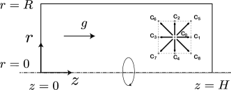
Figure 1: Schematics of the axisymmetric geometry, eventually in presence of gravity or an external force aligned with the z-axis. Schematics also shows the lattice velocities for the D2Q9 model.

The first step in deriving a LBM for axisymmetric multiphase flows is to derive a model that can properly deal with density variations. In particular, the LBM should recover the axisymmetric continuity Eq. (9) and NS Eqs. (10) by means of a Chapman-Enskog (CE) expansion in the long-wavelength and long-timescale limit. In order to derive such a model we start from the 2D LBM with the addition of appropriate space- and time-varying microscopic sources $h_{i}$ (see also Halliday2001 ; Reis2007 ; Reis2007a ; Reis2008 ). We employ the following lattice Boltzmann equation:

$$\begin{split}f_{i}({\textbf{x}}+{\textbf{c}_{i}}\delta t,t+\delta t)&-f_{i}({\textbf{x}},t)=-\frac{1}{\tau}\big{(}f_{i}({\textbf{x}},t)-f^{\mathrm{eq}}_{i}(\rho,{\textbf{u}}^{\mathrm{eq}})\big{)}\\ &~{}~{}~{}~{}+\delta t~{}h_{i}(\textbf{x}+{\textbf{c}_{i}}\delta t/2,t+\delta t/2),\end{split}$$ (11)

where the source terms $h_{i}$, are evaluated at fractional time steps. It can be shown, see Appendix A, that when the additional term $h_{i}$ in Eq. (11) has the following form:

$$h_{i}=W_{i}\Big{(}-\frac{\rho u_{r}}{r}+\frac{1}{c^{2}_{s}}\big{(}c_{iz}H_{z}+c_{ir}H_{r}\big{)}\Big{)},$$ (12)

with

$$H_{z} =\frac{c_{iz}}{r}\bigg{(}\mu\big{(}\partial_{r}u_{z}+\partial_{z}u_{r}\big{)}-\rho u_{r}u_{z}\bigg{)},$$ (13a)

$$H_{r} =\frac{c_{ir}}{r}\bigg{(}2\mu\Big{(}\partial_{r}u_{r}-\frac{u_{r}}{r}\Big{)}-\rho u_{r}^{2}\bigg{)},$$ (13b)

the CE expansion of Eq. (11) provides the axisymmetric version of the continuity and of the NS Eqs.  (9) and (10), respectively. Details on the CE expansion are reported in Appendix A. The equations introduced here are enough to describe a fluid with variable density in axisymmetric geometry. We performed validations of the numerical model (not reported) by observing the behavior of the volume for the case of a droplets approaching the axis. While the 2D volume in the system was not conserved, the properly defined 3D volume was conserved with good accuracy.

II.4 LBM for axisymmetric multiphase flow

With a lattice Boltzmann method capable of handling density variations the additional steps towards the definition of the axisymmetric version of the SC multiphase model only consists in the correct definition of the SC force. The expression for the SC force in 3D is:

$$\textbf{F}({\bf x})=-G\psi({\bf x})\sum_{i}W_{i}\psi({\textbf{x}+\textbf{c}_{i}\delta t})\textbf{c}_{i}.$$ (14)

To find the lattice expression for the axisymmetric case we proceed by passing to the continuum limit, by expressing the continuum force in cylindrical coordinates and then by separating the 2D SC force from the additional axisymmetric contributions.

By means of a Taylor expansion for $\psi({\bf x+c}_{i}\delta t)$ one easily obtains the following continuum expression for the SC force Benzi2006 :

$$\textbf{F}({\bf x}) = -Gc_{s}^{2}\,\delta t\,\psi({\bf x}){\bf{\nabla}}\psi({\bf x})$$ (15)

$$-\frac{G}{2}c_{s}^{4}(\delta t)^{3}\psi({\bf x}){\bf{\nabla}}\big{(}{\bf{\nabla}}^{2}\psi({\bf x})\big{)}$$

$$+\mathcal{O}{(}(\delta t)^{5}).$$

The above force expression is lattice independent and holds true for any 3D coordinate system. We restrict Eq. (15) to the case of axisymmetric flows by expressing both the gradient, ${\bf{\nabla}}$ and the Laplace, ${\bf{\nabla}}^{2}$ operators in cylindrical coordinates given by ${{\bf{\nabla}}\equiv(\partial_{z},\partial_{r})={\bf{\nabla}}_{\mathrm{c}}}$ and ${{\bf{\nabla}}^{2}\equiv(\partial_{zz}+\partial_{rr}+r^{-1}\partial_{r})={\bf{\nabla}}_{\mathrm{c}}^{2}+r^{-1}\partial_{r}}$. Thus, in the axisymmetric case, Eq. (15) reduces to:

$$\textbf{F}({\bf x}) = -Gc_{s}^{2}\,\delta t\,\psi({\bf x}){\bf{\nabla}}_{\mathrm{c}}\psi({\bf x})$$ (16)

$$-\frac{G}{2}c_{s}^{4}(\delta t)^{3}\psi({\bf x}){\bf{\nabla}}_{\mathrm{c}}\big{(}{\bf{\nabla}}_{\mathrm{c}}^{2}\psi({\bf x})\big{)}$$

$$+\textbf{F}^{\mathrm{\gamma,sym}}({\bf x})+\mathcal{O}{(}(\delta t)^{5}).$$

where

$$\textbf{F}^{\mathrm{\gamma,sym}}({\bf x})=-\frac{G}{2}c_{s}^{4}(\delta t)^{3}\psi({\bf x}){\bf{\nabla}}_{\mathrm{c}}\big{(}r^{-1}\partial_{r}\psi({\bf x})\big{)}.$$ (17)

From Eq. (16) we immediately recognize that the first two terms on the right hand side are the ones that one obtains from the Shan-Chen model in 2D. The last term in Eq. (16), $\textbf{F}^{\mathrm{\gamma,sym}}$, is the additional term responsible for the three-dimensionality. This extra contributions needs to be accurately taken into account in order to model the axisymmetric Shan-Chen multiphase systems in 3D. In particular, this term is extremely important in order to correctly implement a 3D surface tension force which responds to curvatures, both along the axis and in the azimuthal direction. The two components of the additional term can be rewritten as:

$${F_{z}^{\mathrm{\gamma,sym}}} = -\frac{G}{2}c_{s}^{4}(\delta t)^{3}\psi r^{-1}\partial_{zr}\psi,$$ (18a)

$${F_{r}^{\mathrm{\gamma,sym}}} = -\frac{G}{2}c_{s}^{4}\psi(\delta t)^{3}\Big{(}r^{-1}\partial_{rr}\psi-r^{-2}\partial_{r}\psi\Big{)}.$$ (18b)

The evaluation of the terms $F_{z}^{\mathrm{\gamma,sym}}$ and $F_{r}^{\mathrm{\gamma,sym}}$ requires an approximation for the derivatives accurate up to order $(\delta t)^{4}$ or higher. Such an accuracy ensures the isotropy of the “reconstructed” 3D axisymmetric Shan-Chen force and thus the isotropy of the resulting surface tension along the interface.

In our implementation we used the following isotropic 5th-order accurate finite difference approximations on D2Q9 lattice (see FIG. 1). For a scalar valued function $\phi(\textbf{x})$ it reads:

$$\partial_{r}\phi(\textbf{x}) = \frac{1}{36}\sum_{i=1}^{8}{\Big{(}8\phi(\textbf{x}+\textbf{c}_{i}\delta t)-\phi(\textbf{x}+2\textbf{c}_{i}\delta t)\Big{)}}c_{ir}$$ (19a)

$$+\mathcal{O}{(}(\delta t)^{5}),$$

$$\partial_{rr}\phi(\textbf{x}) = \frac{1}{36}\sum_{i=1}^{8}{\Big{(}8\partial_{r}\phi(\textbf{x}+\textbf{c}_{i}\delta t)-\partial_{r}\phi(\textbf{x}+2\textbf{c}_{i}\delta t)\Big{)}}c_{ir}$$ (19b)

$$+\mathcal{O}{(}(\delta t)^{5}),$$

$$\partial_{zr}\phi(\textbf{x}) = \frac{1}{12}\Big{(}-\partial_{r}\phi(\textbf{x}+2\textbf{c}_{1}\delta t)+8\partial_{r}\phi(\textbf{x}+\textbf{c}_{1}\delta t)$$ (19c)

$$-8\partial_{r}\phi(\textbf{x}+\textbf{c}_{3}\delta t)+\partial_{r}\phi(\textbf{x}+2\textbf{c}_{3}\delta t)\Big{)}$$

$$+\mathcal{O}{(}(\delta t)^{6}),$$

where $$\partial_{r}\phi(\textbf{x})$$ in Eq. (19c) is approximated as

$$\partial_{r}\phi(\textbf{x}) = \frac{1}{12}\Big{(}-\phi(\textbf{x}+2\textbf{c}_{2}\delta t)+8\phi(\textbf{x}+\textbf{c}_{2}\delta t)$$ (19d)

$$-8\phi(\textbf{x}+\textbf{c}_{4}\delta t)+\phi(\textbf{x}+2\textbf{c}_{4}\delta t)\Big{)}$$

$$+\mathcal{O}{(}(\delta t)^{6}).$$

II.5 Boundary conditions

In axisymmetric flows the boundary conditions for the distribution functions, $f_{i}$, need to be prescribed at all boundaries including the axis. In our approach we impose boundary conditions before the streaming step (pre-streaming). We use mid-grid point specular reflection boundary conditions on the axis sukop_book2006 , this choice allows us to avoid the singularity due to the force terms containing $1/r$. Mid-grid bounce-back or mid-grid specular reflection boundary conditions are used to impose either hydrodynamic no-slip or free-slip conditions at the other walls, respectively sukop_book2006 . In order to impose a prescribed velocity or pressure at inlet and outlet boundaries, we impose the equilibrium distribution functions, $f^{\mathrm{eq}}_{i}$, evaluated using the desired hydrodynamic velocity and density values. For our LBM simulations we use unit time step $({\delta t=1})$ and unit grid spacing ${(\delta z=\delta r=1)}$, hence the length can be measured in terms of the number of nodes. We are using symmetry boundary condition is used for the derivative evaluation in (13) and (17) at the axis. For other three boundaries we impose the derivatives terms to be zero.

III Numerical validation for single-phase axisymmetric LBM

Here we present the validation of the axisymmetric LBM for single-phase flow simulations by comparing it with analytical solutions for the test cases: the axial flow through a tube and the outward radial flow between two parallel discs. These two tests complement each other because they correspond to flows parallel and orthogonal to the axis, respectively. Both flow problems have analytical steady state solutions that help us to validate the accuracy of the axial and radial component of the velocity. All physical quantities in this manuscript, unless otherwise stated, are reported in lattice units (l.u.), the relaxation time has been keep fixed for all the simulations, $\tau$ = 1, and the simulations have been carried out on a rectangular domain of size $H\times R=N_{z}\times N_{r}$. The steady state in the following single-phase simulations is defined when the total kinetic energy of the system, ${E_{ke}=\pi\sum_{N_{z}}(\sum_{N_{r}}r\rho|\textbf{u}|^{2}})$, becomes constant up to the machine precision.

III.0.1 Flow through a pipe

In this test we consider the constant-density flow of a fluid with density, $\rho$, kinematic viscosity, $\nu$, flowing inside a circular pipe of radius $R$. The flow is driven by a constant body force, ${\rho g}$, along to the axis of the pipe. The schematic illustration of the flow geometry is presented in FIG. 1. Assuming $u_{r}(z,r)=0$ and no-slip condition on the inner surface $(r=R)$ of the pipe, the steady state solution for the axisymmetric NS Eq. (10) for this problem is given by Middleman_book1995 :

$$u_{z}(z,r) =U_{1}\left[1-\left(\frac{r}{R}\right)^{2}\right],$$ (20)

where ${U_{1}=u_{r}(z,0)=gR^{2}/(4\nu)}$, is the maximum velocity in the pipe.

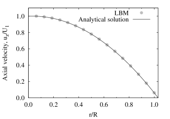
Figure 2: A comparison of the axial velocity profile as obtained form the LBM simulations (circles) versus the analytical solution (solid line) Eq. (20). Simulation parameters: $N_{z}\times N_{r}=16\times 16$, $R=N_{r}$, $\rho$ = 1, $\nu$ = 0.167, $g=10^{-5}$, $U_{1}=u_{z}(0)=3.84\times 10^{-3}$ .

For the LBM simulation we used the no-slip boundary condition at the inner surface of the pipe, and periodic boundary conditions at the open ends of the pipe. The body force $g=10^{-5}$ is applied at each node of the simulation domain. The LBM simulations are carried out till the simulation reaches its steady state. The result of the LBM simulation shown in FIG. 2 is in very good agreement with the analytical solution in Eq. (20). This validates the single phase axisymmetric LBM for the case where there is no velocity in the radial direction.

III.0.2 Outward radial flow between two parallel discs

Another important test to validate the single-phase axisymmetric LBM is the simulation of the outward radial flow between two parallel discs separated by a distance $H$. The schematic of the flow setup for this problem is reported in FIG. 3.

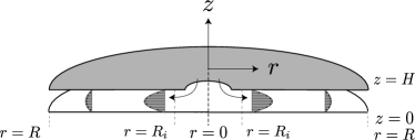
Figure 3: Schematics of the physical setup to study outward radial flow between two parallel discs. The arrows show the direction of the inlet mass flow. The LBM is used to simulate the flow domain $0\leq z\leq H$ , $R_{i}\leq r\leq R$. We assume that the flow is fully developed for $r\geq R_{i}$ and hence the axial velocity $u_{z}$ vanishes in this region.

Assuming $u_{z}(z,r)=0$ for $R_{i}\leq r\leq R$, the no-slip boundary condition on the discs and a constant mass flow rate $Q$ along the radial direction, the solution of the NS Eq. (10) corresponding to this problem is given by Middleman_book1995 :

$$u_{r}(z,r)=-U_{2}\left(\frac{4R_{i}}{H^{2}}\right)\frac{z(z-H)}{r},$$ (21)

where ${U_{2}=u_{r}(H/2,R_{i})=3Q/(4\pi R_{i}H)}$. The LBM results shown in FIG. 4 are carried out for the flow domain $R_{i}\leq r\leq R,0\leq z\leq H$ and using the no-slip boundary condition along the discs. The velocity profile given by Eq. (21) is applied at the inlet boundary while the outlet is considered as an open boundary. The LBM results shown in FIG. 4 are in a very good agreement with the analytical solution Eq. (21). This validates the single phase axisymmetric LBM for the case of a radial velocity.

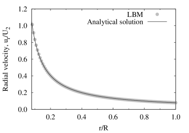
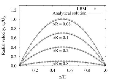
Figure 4: A comparison of the radial velocity profile, $u_{r}$, as obtained form LBM simulations (circles) versus the analytical solution (solid lines) of Eq. (21). Simulation parameters: $N_{z}\times N_{r}=32\times 120$, $R=N_{r}-0.5$, $H=N_{z}$, $R_{i}=9.5$, $\rho=1$, $\nu=0.167$, $Q=0.5$ and $U_{2}=3.93\times 10^{-4}$. Top figure shows the comparison at $z=15.5$. Bottom figure from top to bottom shows the curves correspond to the radial distances $r/R=0.8,0.2,0.1$ and $0.08$.

IV Numerical validation for axisymmetric multiphase model

In this section we present the validation for our axisymmetric multiphase LBM for three standard test cases: Laplace law, oscillation of a viscous drop and the Rayleigh-Plateau (RP) instability.

IV.0.1 Laplace test

In this validation we compare the in-out pressures differences for different droplet radii. According to the Laplace law the in-out pressure difference, $\Delta p$, for a droplet of radius $R_{\mathrm{D}}$ is given by

$$\Delta p=\frac{2\gamma_{\mathrm{lv}}}{R_{\mathrm{D}}},$$ (22)

where $\gamma_{\mathrm{lv}}$ is the liquid-vapor interfacial tension. For this validation we first estimate the value of the surface tension using Eq. (7) (Guo scheme Guo2002 ) and Eq. (8) (SC scheme Shan1994 ) for both 2D and axisymmetric LBM. The data obtained from these simulations are reported in TABLE 1.

	SC		Guo
G	$\tilde{\gamma}_{\mathrm{lv}}^{\mathrm{2D}}$	$\tilde{\gamma}_{\mathrm{lv}}^{\mathrm{axis}}$	$\gamma_{\mathrm{lv}}^{\mathrm{2D}}$	$\gamma_{\mathrm{lv}}^{\mathrm{axis}}$
-4.5	0.0220	0.0220	0.0135	0.0136
-5.0	0.0579	0.0579	0.0376	0.0378
-5.5	0.0995	0.0996	0.0681	0.0683

Table 1: Surface tension evaluated using Eq. (8) (column 2,3) and Eq. (7) (column 4,5). Here $\gamma_{\mathrm{lv}}^{\mathrm{2D}},\gamma_{\mathrm{lv}}^{\mathrm{axis}}$ denote the surface tensions obtained from 2D and axisymmetric LBM, respectively. Simulation parameters: ${N_{z}\times N_{r}=1\times 64}$, $\tau=1$, initial interface position, $r=32$.

Both the Guo and SC scheme are consistent with the fact that for the SC model the surface tension should only depends on the value of the interaction parameter, $G$.

In the next step we do a series of axisymmetric LBM simulation for different droplet radii and measure the in-out pressure difference. When comparing the in-out pressure difference for a drop (Laplace test) and the pressure drop given by Eq. (22), we find that the maximum relative error in pressure difference for Guo scheme Guo2002 and SC scheme Shan1994 is 2% and 20%, respectively. This difference might be due to following reason.

IV.0.2 Oscillating droplet

Here we consider the dynamics of the oscillation of an axisymmetric droplet in order to validate the axisymmetric multiphase LBM. We compare the frequency of the oscillation of the droplet obtained from the LBM simulation with the analytical solution reported in Miller and Scriven Miller1968 . The frequency of the second mode for the oscillation of a liquid droplet immersed in another fluid is given by:

$$\omega_{2}=\omega_{2}^{\ast}-0.5\alpha(\omega_{2}^{\ast})^{1/2}+0.25\alpha^{2},$$ (23)

where

$$\omega_{2}^{\ast}=\sqrt{\frac{24\gamma_{\mathrm{lv}}}{R_{\mathrm{D}}^{3}(2\rho_{v}+3\rho_{l})}},$$

and $R_{\mathrm{D}}$ is the radius of the drop at equilibrium, $\gamma_{\mathrm{lv}}$ is the surface tension, $\rho_{l},\rho_{v}$ are the densities of the liquid and vapor phases, respectively. The parameter $\alpha$ is given by:

$$\alpha=\frac{25\sqrt{\nu_{l}\nu_{v}}\rho_{l}\rho_{v}}{\sqrt{2}R_{\mathrm{D}}(2\rho_{v}+3\rho_{l})(\sqrt{\nu_{l}}\rho_{l}+\sqrt{\nu_{v}}\rho_{v})},$$

where $\nu_{l},\nu_{v}$ are the kinematic viscosities of the liquid and vapor phase Miller1968 .

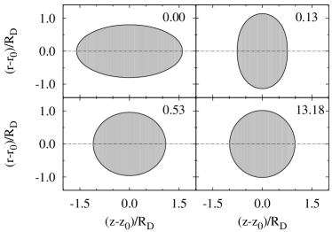
Figure 5: Time evolution of the shape of an ellipsoidal droplet immersed in a fluid with different density. Simulation parameters: $N_{z}\times N_{r}=320\times 128$, $G=-6$. $\rho_{l}$ = 2.65 , $\rho_{v}$ = 0.075, $(z_{0},r_{0})=(160.0,0.5)$. Labels indicate the time corresponding to the different droplet shapes.

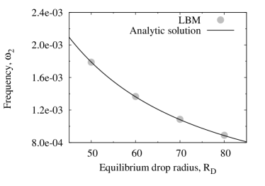
Figure 6: Top panel: amplitude, $A(t)$, of the oscillations versus time, $t$, for different equilibrium droplet radii, $R_{\mathrm{D}}$. Solid lines are obtained by fitting the function, ${g(t)=R_{\mathrm{D}}+a\exp(-bt)\sin(\omega_{2}t+d),}$ to the data obtained from LBM simulations. Bottom panel: dimensionless frequency of the second mode of oscillation, $\omega_{2}$, versus the equilibrium droplet radius, $R_{\mathrm{D}}$. Simulation parameters: $N_{z}\times N_{r}=320\times 128$, $G=-6$.

In the LBM simulations for this test we use the free-slip boundary condition at the top boundary and periodic boundary conditions at the left and right boundaries. The LBM simulations are initialized with an axisymmetric ellipsoid, ${(z/R_{a})^{2}+(r/R_{b})^{2}=1}$, where $R_{a},R_{b}$ are the intercepts on the $z$ and $r$-axis, respectively, with total volume $4\pi R_{a}R_{b}^{2}/3$. Due to the surface tension, the ellipsoidal droplet oscillates and due to viscous damping it does finally attain an equilibrium spherical shape with radius $R_{\mathrm{D}}=(R_{a}R_{b}^{2})^{1/3}$ (due to volume conservation). The time evolution of one of these LBM simulations is shown in FIG. 5. The time is measured in the capillary time scale, ${t_{cap}=\sqrt{R_{\mathrm{D}}^{3}\rho_{l}/\gamma_{\mathrm{lv}}}}$. The LBM simulations are performed to validate the effect of the droplet size, $R_{\mathrm{D}}$, on the frequency of oscillation, $\omega_{2}$. In order to calculate the frequency of the oscillation we first measure the length of the intercept on the $r$-axis as a function of time, $A(t)$ with $A(t=0)=R_{b}$, and then we fit the function ${g(t)=R_{\mathrm{D}}+a\exp(-bt)\sin(\omega_{2}t+d),}$ (see FIG. 6). We find that the numerical estimation of the frequency of the oscillation of the droplet is in excellent agreement with the theoretically expected value, with a maximum relative error of approximatly 1% (see FIG. 6).

IV.0.3 Rayleigh - Plateau (RP) instability

The last problem that we consider for the validation is the breakup of a liquid thread into multiple droplets. The problem was first studied experimentally by Plateau Plateau1873 and later theoretically by Lord Rayleigh Rayleigh1879 , and is currently referred to as Rayleigh-Plateau (RP) instability. The RP instability has been extensively studied experimentally, theoretically and numerically Plateau1873 ; Rayleigh1879 ; Lafrance1975 ; Tomotika1935 . Moreover, the problem is fully axisymmetric and therefore suitable for the validation of our multiphase axisymmetric LBM model.

In this validation we check the instability criterion: a liquid cylinder of radius $R_{\mathrm{C}}$ is unstable, if the wavelength of a disturbance, $\lambda$, on the surface of a liquid cylinder is longer then its circumference ${2\pi R_{\mathrm{C}}}$. Moreover, we compare the radius of the resulting drops with experimental Rutland1971 and numerical data Driessen2011 .

For the LBM simulations we use free-slip boundary condition at the top boundary and periodic boundary conditions at left and right boundaries. The LBM simulations are performed in a domain of size ${N_{z}\times N_{r}=\lambda\times 450}$. The wavelength, $\lambda$, of the noise runs over 576, 768, 1024, 1280, 1536 and 1792 for different wavenumbers, $\kappa=2\pi/\lambda$. We represent the wavenumber in dimensionless form as $\kappa^{*}=\kappa R_{\mathrm{C}}$. The SC interaction parameter, ${G=-6.0}$, liquid density $\rho_{l}=2.68$, vapor density $\rho_{v}=0.078$, surface tension $\gamma_{\mathrm{lv}}=0.141$ and kinematic viscosity $\nu=0.016$ are fixed for these simulations. For these parameters the Ohnesorge number, ${Oh=\nu\sqrt{\rho_{l}/(\gamma_{\mathrm{lv}}R_{\mathrm{C}}})=0.09}$. The axial velocity field in the liquid cylinder is initialized by using sinusoidal velocity field as ${u_{z}(z,r)=\epsilon_{u}\sin(2\pi z/\lambda)}$. For our LBM simulation we use $\epsilon_{u}<5\times 10^{-3}$.

The time evolution of the RP instability corresponding to two different wavenumber ${\kappa^{*}=2\pi R_{\mathrm{C}}/\lambda}$ is shown in FIG. 7. The time is measured in the capillary time scale, ${t_{cap}=\sqrt{R_{\mathrm{C}}^{3}\rho_{l}/\gamma_{\mathrm{lv}}}}$. In our simulations we find that the cylinder breaks up into two or more droplets as long as the condition $\kappa^{*}<1$ is satisfied (corresponding to the RP instability criterion, ${2\pi R_{\mathrm{C}}<\lambda}$). Furthermore, the comparisons of drop sizes for different wavenumber shown in FIG. 8 is in excellent agreement with the results of the slender jet approximation model (SJ) Driessen2011 and with experimental data Rutland1971 .

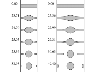
Figure 7: Growth of the Rayleigh-Plateau instability with time. Left panel: $\kappa^{*}$ = 0.65; right panel: $\kappa^{*}$ = 0.39. Labels on figures indicate the corresponding dimensionless time, $t/t_{cap}$.

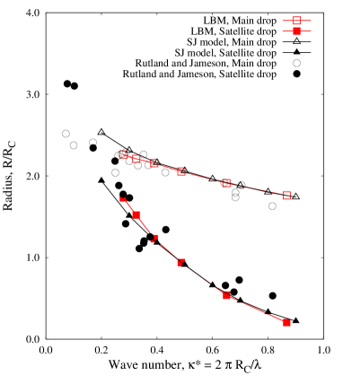
Figure 8: Dimensionless wave-number $\kappa^{*}$ versus dimensionless droplet radius, $R/R_{\mathrm{C}}$. Triangles markers represents the data obtained from the SJ model for $Oh=0.1$ Driessen2011 , circle markers represents the data from experiments Rutland1971 and square markers represents data from the axisymmetric LBM simulations for $Oh=0.09$.

V Conclusions

In the present manuscript we introduced a novel axisymmetric LBM formulation that can be employed for single-phase as well as for multiphase flows. The multiphase model is the widely employed Shan-Chen model and the axisymmetric version here described is particularly convenient as it allows one to easily switch from 3D to 2D axisymmetric simulations while maintaing the usual Shan-Chen parameters (i.e. densities and coupling strength). The lattice Boltzmann axisymmetric model allows for the solution of multiphase flows at the computational cost of a 2D simulation. One particular interesting application comes from the possibility of increasing the system size, thus reducing the relative size of the LBM diffuse interface with respect to all other length scales in the flow. We presented several validations for single-phase as well as for multiphase flows. In the case of multiphase flows we have quantitatively validated the mass conservation and the dynamics of an axially symmetric oscillating droplet. The constraint of axis-symmetry may partially be relaxed by models that keep into account azimuthal perturbation to lowest order, this will be the subject of future work.

Appendix A Chapman-Enskog on modified LBM

The modified lattice Boltzmann Eq. (11) for the distribution function $f_{i}(\textbf{x},t)$ reads

$$\begin{split}f_{i}({\textbf{x}}+{\textbf{c}_{i}}\delta t,t+\delta t)&-f_{i}({\textbf{x}},t)=-\frac{1}{\tau}\big{(}f_{i}({\textbf{x}},t)-f^{\mathrm{eq}}_{i}(\rho,{\textbf{u}}^{\mathrm{eq}})\big{)}\\ &~{}~{}~{}~{}+\delta t~{}h_{i}(\textbf{x}+{\textbf{c}_{i}}\delta t/2,t+\delta t/2).\end{split}$$ (24)

where $h_{i}$ is the source terms, $\textbf{c}_{i}$ is the lattice velocities $\tau$ is the relaxation parameter and $f^{\mathrm{eq}}_{i}$ is the discrete second order approximation of the Maxwell-Boltzmann distribution function

$$f^{\mathrm{eq}}_{i}(\rho,\textbf{u}) = W_{i}\rho\bigg{[}1+\frac{1}{c_{s}^{2}}(\textbf{c}_{i}\cdot\textbf{u})+\frac{1}{2c_{s}^{4}}(\textbf{c}_{i}\cdot{\textbf{u}}^{\mathrm{eq}})^{2}$$ (25)

$$-\frac{1}{2c_{s}^{2}}|{\textbf{u}}^{\mathrm{eq}}|^{2}\bigg{]},$$

where $c_{s}$ is the speed of sound and $W_{i}$’s are the weight factors to ensure the symmetry of the lattice. For the D2Q9 LB model with BGK collision operator the speed of sound, $c_{s}=\sqrt{1/3}$, $W_{0}=4/9$, $W_{i}=1/9$ for $i=1,2,3,4$ and $W_{i}=1/36$ for $i=5,6,7,8$. In general these weights satisfy following symmetry

$$\sum_{i}{W_{i}} =1, \sum_{i}{W_{i}c_{i\alpha}} =0,$$

$$\sum_{i}{W_{i}c_{i\alpha}c_{i\beta}} =c_{s}^{2}\delta_{\alpha\beta}, \sum_{i}{W_{i}c_{i\alpha}c_{i\beta}c_{i\gamma}} =0,$$

$$\sum_{i}{W_{i}c_{i\alpha}c_{i\beta}c_{i\gamma}c_{i\delta}}=c_{s}^{4}\big{(}\delta_{\alpha\beta}\delta_{\gamma\delta}+\delta_{\alpha\gamma}\delta_{\beta\delta}+\delta_{\alpha\delta}\delta_{\beta\gamma}),$$ (26)

$$\sum_{i}{W_{i}c_{i\alpha}c_{i\beta}c_{i\gamma}c_{i\delta}c_{i\eta}}=0.$$

The density, $\rho$ and momentum, ($\rho\textbf{u}$) are given by the zeroth and first moment of the distribution function respectively, $i.e.,$

$$\rho(\textbf{x},t) =\sum_{i}{f_{i}(\textbf{x},t)},$$ (27a)

$$(\rho\textbf{u})(\textbf{x},t) =\sum_{i}{\textbf{c}_{i}f_{i}(\textbf{x},t)}.$$ (27b)

In absence of any external force, ${{\textbf{u}}^{\mathrm{eq}}=\textbf{u}}$. In order to establish a relation between the LB Eq. (24) continuity Eq. (9) and the NS equations (10) it is necessary to separate different time scales. We distinguish between slow and fast varying quantities by using two time scales and one space scale Wolf-gladrow2005 . We expand the time and space derivative (${\bf{\nabla}}_{\mathrm{c}}:$ the gradient operator in the Cartesian coordinate system) using a parameter $\varepsilon$ as

$$\partial_{t}=\varepsilon\partial_{t}^{(1)}+\varepsilon^{2}\partial_{t}^{(2)}+\mathcal{O}{(}\varepsilon^{3}),{\bf{\nabla}}_{\mathrm{c}}=\varepsilon{\bf{\nabla}}_{\mathrm{c}}^{(1)}+\mathcal{O}{(}\varepsilon^{2}),$$ (28)

and the distribution function, $f_{i}$ as

$$f_{i}=f_{i}^{(0)}+\varepsilon f_{i}^{(1)}+\varepsilon^{2}f_{i}^{(2)}+\mathcal{O}{(}\varepsilon^{3}).$$ (29)

The zeroth order contribution $f_{i}^{(0)}$ is exactly the same as the equilibrium distribution function,$f^{\mathrm{eq}}_{i}$. The first and second order perturbations do not contribute to and momentum Wolf-gladrow2005 :

$$\sum_{i}{f_{i}^{(1)}} =\sum_{i}{f_{i}^{(2)}}=0,$$ (30a)

$$\sum_{i}{\textbf{c}_{i}f_{i}^{(1)}} =\sum_{i}{\textbf{c}_{i}f_{i}^{(2)}}=0.$$ (30b)

The source term $h_{i}$ does not have any zeroth order contribution and is expanded as

$$h_{i}=\varepsilon h_{i}^{(1)}+\varepsilon^{2}h_{i}^{(2)}+\mathcal{O}{(}\varepsilon^{3}).$$ (31)

Taylor series of $f_{i}$ and $h_{i}$ around $(\textbf{x},t)$ are given by

$$f_{i}(\textbf{x}+\textbf{c}_{i}\delta t,t+\delta t) = f_{i}(\textbf{x},t)+\delta t(\partial_{t}+c_{i\alpha}\partial_{\alpha})f_{i}(\textbf{x},t)+\frac{(\delta t)^{2}}{2}(\partial_{t}+c_{i\alpha}\partial_{\alpha})^{2}f_{i}(\textbf{x},t)+\mathcal{O}{(}({\delta t})^{3}),$$ (32)

$$h_{i}(\textbf{x}+\textbf{c}_{i}\delta t/2,t+\delta t/2) = h_{i}(\textbf{x},t)+\frac{\delta t}{2}(\partial_{t}+c_{i\alpha}\partial_{\alpha})h_{i}(\textbf{x},t)+\frac{1}{2}\left(\frac{\delta t}{2}\right)^{2}(\partial_{t}+c_{i\alpha}\partial_{\alpha})^{2}h_{i}(\textbf{x},t)+\mathcal{O}{(}({\delta t})^{3}),$$ (33)

where $c_{i\alpha}$ is the $\alpha$-th component of $\textbf{c}_{i}$, and $\partial_{\alpha}$ represents the partial derivative with respect to $\alpha$-th component of x. Indices $\alpha,\beta,\gamma,\delta$ used in the following derivation ranges over the set $\{z,r\}$, and when an index appears twice in a single term it represents the standard Einstein summation convention. Using Eq. (28),(29),(32), and (33) in (24) and rearranging the terms we obtain a series in $\varepsilon$

$$\begin{split}\varepsilon\left[\delta t\left(\partial_{t}^{(1)}f_{i}^{(0)}+c_{i\alpha}\partial_{\alpha}^{(1)}f_{i}^{(0)}\right)\right]+\varepsilon^{2}\left[\delta t\left(\partial_{t}^{(2)}f_{i}^{(0)}+\partial_{t}^{(1)}f_{i}^{(1)}+c_{i\alpha}\partial_{\alpha}^{(1)}f_{i}^{(1)}\right)+\frac{(\delta t)^{2}}{2}\left(\partial_{t}^{(1)}\partial_{t}^{(1)}f_{i}^{(0)}+c_{i\alpha}c_{i\beta}\partial_{\alpha}^{(1)}\partial_{\beta}^{(1)}f_{i}^{(0)}\right.\right.\\ \left.\left.+2c_{i\alpha}\partial_{t}^{(1)}\partial_{\alpha}^{(1)}f_{i}^{(0)}\right)\right]=\varepsilon\left[-\frac{1}{\tau}f_{i}^{(1)}+\delta t~{}h_{i}^{(1)}\right]+\varepsilon^{2}\left[-\frac{1}{\tau}f_{i}^{(2)}+\delta t~{}h_{i}^{(2)}+\frac{(\delta t)^{2}}{2}\Big{(}\partial_{t}^{(1)}+c_{i\alpha}\partial_{\alpha}^{(1)}\Big{)}h_{i}^{(1)}\right]+\mathcal{O}{(}\varepsilon^{3}).\end{split}$$ (34)

Comparing the coefficients of $\varepsilon$, $\varepsilon^{2}$ and omitting $\varepsilon^{3}$ terms in Eq. (34) gives us

$$\delta t\left(\partial_{t}^{(1)}f_{i}^{(0)}+c_{i\alpha}\partial_{\alpha}^{(1)}f_{i}^{(0)}\right)=-\frac{1}{\tau}f_{i}^{(1)}+\delta t~{}h_{i}^{(1)},$$ (35)

$$\begin{split}\delta t\left(\partial_{t}^{(2)}f_{i}^{(0)}+\partial_{t}^{(1)}f_{i}^{(1)}+c_{i\alpha}\partial_{\alpha}^{(1)}f_{i}^{(1)}\right)+\frac{(\delta t)^{2}}{2}\left(\partial_{t}^{(1)}\partial_{t}^{(1)}f_{i}^{(0)}+c_{i\alpha}c_{i\beta}\partial_{\alpha}^{(1)}\partial_{\beta}^{(1)}f_{i}^{(0)}+2c_{i\alpha}\partial_{t}^{(1)}\partial_{\alpha}^{(1)}f_{i}^{(0)}\right)\\ =-\frac{1}{\tau}f_{i}^{(2)}+\delta t~{}h_{i}^{(2)}+\frac{(\delta t)^{2}}{2}\Big{(}\partial_{t}^{(1)}+c_{i\alpha}\partial_{\alpha}^{(1)}\Big{)}h_{i}^{(1)},~{}~{}~{}~{}~{}~{}~{}~{}~{}\end{split}$$ (36)

respectively. In the following steps of the CE expansion we will take the zeroth and first lattice velocity moments of Eqs. (35) and (36). The zeroth moment of Eqs. (35) and (36) will give us the mass conservation up to $\varepsilon$ and $\varepsilon^{2}$ order terms, respectively, and the first moment of Eqs. (35) and (36) will give us the momentum conservation up to $\varepsilon$ and $\varepsilon^{2}$ order terms, respectively. Finally by using Eq. (28) we will obtain equations that conserves the hydrodynamic mass and momentum up to $\mathcal{O}{(}\varepsilon^{2})$ perturbations in $f_{i}$.

The zeroth and first order moments of Eq. (35) along with Eqs. (27) and (30)

$$\partial_{t}^{(1)}\rho+\partial_{\alpha}^{(1)}(\rho u_{\alpha}) =\sum_{i}h_{i}^{(1)},$$ (37)

$$\partial_{t}^{(1)}(\rho u_{\beta})+\partial_{\alpha}^{(1)}\Pi_{\alpha\beta}^{(0)} =\sum_{i}c_{i\beta}h_{i}^{(1)},$$ (38)

. $\Pi_{\alpha\beta}^{(0)}$ is the zeroth order stress tensor, and

$$\Pi_{\alpha\beta}^{(0)}\equiv\sum_{i}c_{i\alpha}c_{i\beta}f_{i}^{(0)}=\rho\left(c_{s}^{2}\delta_{\alpha\beta}+u_{\alpha}u_{\beta}\right).$$ (39)

$$\begin{split}\delta t\bigg{(}\partial_{t}^{(2)}\sum_{i}f_{i}^{(0)}+\partial_{t}^{(1)}\sum_{i}f_{i}^{(1)}+\partial_{\alpha}^{(1)}\sum_{i}c_{i\alpha}f_{i}^{(1)}\bigg{)}+\frac{(\delta t)^{2}}{2}\bigg{(}\partial_{t}^{(1)}\partial_{t}^{(1)}\sum_{i}f_{i}^{(0)}+\partial_{\alpha}^{(1)}\partial_{\beta}^{(1)}\sum_{i}c_{i\alpha}c_{i\beta}f_{i}^{(0)}\\ +2\partial_{t}^{(1)}\partial_{\alpha}^{(1)}\sum_{i}c_{i\alpha}f_{i}^{(0)}\bigg{)}=-\frac{1}{\tau}\sum_{i}f_{i}^{(2)}+\delta t\sum_{i}h_{i}^{(2)}+\frac{(\delta t)^{2}}{2}\bigg{(}\partial_{t}^{(1)}\sum_{i}h_{i}^{(1)}+\partial_{\alpha}^{(1)}\sum_{i}c_{i\alpha}h_{i}^{(1)}\bigg{)}.~{}~{}~{}~{}~{}~{}~{}~{}~{}\end{split}$$

Using Eqs. (30), (27) and (39) we get

$$\partial_{t}^{(2)}\rho+\frac{\delta t}{2}\left(\partial_{t}^{(1)}\partial_{t}^{(1)}\rho+\partial_{\alpha}^{(1)}\partial_{\beta}^{(1)}\Pi_{\alpha\beta}^{(0)}+2\partial_{t}^{(1)}\partial_{\alpha}^{(1)}\big{(}\rho u_{\alpha}\big{)}\right) = \sum_{i}h_{i}^{(2)}+\frac{\delta t}{2}\Big{(}\partial_{t}^{(1)}\sum_{i}h_{i}^{(1)}+\partial_{\alpha}^{(1)}\sum_{i}c_{i\alpha}h_{i}^{(1)}\Big{)}.$$

$$\partial_{t}^{(2)}\rho+\frac{\delta t}{2}\bigg{(}\partial_{t}^{(1)}\left(\partial_{t}^{(1)}\rho+\partial_{\alpha}^{(1)}(\rho u_{\alpha})\right)+\partial_{\alpha}^{(1)}\left(\partial_{t}^{(1)}(\rho u_{\alpha})+\partial_{\beta}^{(1)}\Pi_{\alpha\beta}^{(0)}\right)\bigg{)} = \sum_{i}h_{i}^{(2)}+\frac{\delta t}{2}\bigg{(}\partial_{t}^{(1)}\sum_{i}h_{i}^{(1)}+\partial_{\alpha}^{(1)}\sum_{i}c_{i\alpha}h_{i}^{(1)}\bigg{)}.$$

Finally using Eq. (37) and (LABEL:eq:firstmom_eps) we get

$$\partial_{t}^{(2)}\rho+\frac{\delta t}{2}\bigg{(}\partial_{t}^{(1)}\sum_{i}h_{i}^{(1)}+\partial_{\alpha}^{(1)}\sum_{i}c_{i\alpha}h_{i}^{(1)}\bigg{)} = \sum_{i}h_{i}^{(2)}+\frac{\delta t}{2}\bigg{(}\partial_{t}^{(1)}\sum_{i}h_{i}^{(1)}+\partial_{\alpha}^{(1)}\sum_{i}c_{i\alpha}h_{i}^{(1)}\bigg{)}.$$ (40)

Rearranging the terms of Eq. (40) gives

$$\partial_{t}^{(2)}\rho = \sum_{i}h_{i}^{(2)}.$$ (41)

We assume that the source term $h_{i}^{2}$ does not change the density at diffusive time scale, $i.\,e.$

$$\sum_{i}h_{i}^{(2)}=0.$$ (42)

Using the relation $\varepsilon$(37)+ $\varepsilon^{2}$ (41) we get

$$\partial_{t}\rho+\partial_{\alpha}(\rho u_{\alpha})=\varepsilon\sum_{i}h_{i}^{(1)}+\varepsilon^{2}\sum_{i}h_{i}^{(2)}.$$ (43)

If we choose

$$\varepsilon h_{i}^{(1)} = -\frac{W_{i}\rho u_{r}}{r},$$ (44)

then

$$\sum_{i}h_{i}^{(1)} =-\frac{1}{\varepsilon}\frac{\rho u_{r}}{r},$$ (45a)

$$\sum_{i}c_{i\alpha}h_{i}^{(1)} =0,$$ (45b)

$$\sum_{i}c_{i\alpha}c_{i\beta}h_{i}^{(1)} =-c_{s}^{2}\frac{1}{\varepsilon}\frac{\rho u_{r}}{r}\delta_{\alpha\beta}.$$ (45c)

the Eqs. (43), (45a) and (42) gives us

$$\partial_{t}\rho+\partial_{\alpha}(\rho u_{\alpha})=-\frac{\rho u_{r}}{r}.$$ (46)

Eq. (46) is the axisymmetric continuity Eq. (9).

we take the first moment of Eq. (36)

$$\begin{split}\delta t\bigg{(}\partial_{t}^{(2)}\sum_{i}c_{i\gamma}f_{i}^{(0)}+\partial_{t}^{(1)}\sum_{i}c_{i\gamma}f_{i}^{(1)}+\partial_{\alpha}^{(1)}\sum_{i}c_{i\alpha}c_{i\gamma}f_{i}^{(1)}\bigg{)}+\frac{(\delta t)^{2}}{2}\bigg{(}\partial_{t}^{(1)}\partial_{t}^{(1)}\sum_{i}c_{i\gamma}f_{i}^{(0)}+\partial_{\alpha}^{(1)}\partial_{\beta}^{(1)}\sum_{i}c_{i\alpha}c_{i\beta}c_{i\gamma}f_{i}^{(0)}\\ +2\partial_{t}^{(1)}\partial_{\alpha}^{(1)}\sum_{i}c_{i\alpha}c_{i\gamma}f_{i}^{(0)}\bigg{)}=-\frac{1}{\tau}\sum_{i}c_{i\gamma}f_{i}^{(2)}+\delta t~{}\sum_{i}c_{i\gamma}h_{i}^{(2)}+\frac{(\delta t)^{2}}{2}\bigg{(}\partial_{t}^{(1)}\sum_{i}c_{i\gamma}h_{i}^{(1)}+\frac{\delta t}{2}\partial_{\alpha}^{(1)}\sum_{i}c_{i\gamma}c_{i\alpha}h_{i}^{(1)}\bigg{)},~{}~{}~{}~{}~{}~{}~{}~{}~{}\end{split}$$

using Eqs. (27), (30) and (45a) we get

$$\begin{split}\partial_{t}^{(2)}(\rho u_{\gamma})+\partial_{\alpha}^{(1)}\Pi_{\alpha\gamma}^{(1)}+\frac{\delta t}{2}\left(\partial_{t}^{(1)}\partial_{t}^{(1)}(\rho u_{\gamma})+\partial_{\alpha}^{(1)}\partial_{\beta}^{(1)}P_{\alpha\beta\gamma}^{(0)}+2\partial_{t}^{(1)}\partial_{\alpha}^{(1)}\Pi_{\alpha\gamma}^{(0)}\right)=\sum_{i}c_{i\gamma}h_{i}^{(2)}-c_{s}^{2}\frac{1}{\varepsilon}\partial_{\gamma}^{(1)}\Big{(}\frac{\rho u_{r}}{r}\Big{)},\end{split}$$ (47)

where

$$P_{\alpha\beta\gamma}^{(0)} \equiv\sum_{i}c_{i\alpha}c_{i\beta}c_{i\gamma}f_{i}^{(0)},$$ (48)

$$\Pi_{\alpha\gamma}^{(1)} \equiv\sum_{i}{c_{i\alpha}c_{i\gamma}f_{i}^{(1)}}.$$ (49)

Using Eq. (25) and (A) in Eq. (48) we get

$$P_{\alpha\beta\gamma}^{(0)} =\frac{1}{c_{s}^{2}}\sum_{i}{W_{i}c_{i\alpha}c_{i\beta}c_{i\gamma}c_{i\delta}(\rho u_{\delta})}$$

$$=c_{s}^{2}\Big{(}\delta_{\alpha\beta}(\rho u_{\gamma})+\delta_{\beta\gamma}(\rho u_{\alpha})+\delta_{\alpha\gamma}(\rho u_{\beta})\Big{)},$$ (50)

and Eq. (35) in Eq. (49) gives

$$\Pi_{\alpha\gamma}^{(1)} =\delta t~{}\tau\sum_{i}{c_{i\alpha}c_{i\gamma}\left(h_{i}^{(1)}-c_{i\delta}\partial_{\delta}^{(1)}f_{i}^{(0)}-\partial_{t}^{(1)}f_{i}^{(0)}\right)}$$

$$=\delta t~{}\tau\sum_{i}c_{i\alpha}c_{i\gamma}h_{i}^{(1)}-\delta t~{}\tau\left(\partial_{\delta}^{(1)}P^{(0)}_{\alpha\gamma\delta}+\partial_{t}^{(1)}\Pi^{(0)}_{\alpha\gamma}\right).$$ (51)

Substituting Eqs. (LABEL:eq:firstmom_eps) and (A) in (47) and rearranging gives

$$\begin{split}&\partial_{t}^{(2)}(\rho u_{\gamma})-\delta t\left(\tau-\frac{1}{2}\right)\left(\partial_{\alpha}^{(1)}\partial_{\delta}^{(1)}P^{(0)}_{\alpha\gamma\delta}+\partial_{t}^{(1)}\partial_{\alpha}^{(1)}\Pi_{\alpha\gamma}^{(0)}\right)\\ &=c_{s}^{2}\frac{1}{\varepsilon}\delta t\left(\tau-\frac{1}{2}\right)\partial_{\gamma}^{(1)}\Big{(}\frac{\rho u_{r}}{r}\Big{)}+\sum_{i}c_{i\gamma}h_{i}^{(2)}.\end{split}$$ (52)

In order to obtain the NS Eq. (10) from the lattice Boltzmann Eq. (24) it is necessary that the hydrodynamic velocity the low Mach number, $Ma$ condition $i.e.~{}\mathcal{O}{(}Ma^{3})$ terms are very small and can be neglected from the Eq. (52). The third order velocity appears only in the expression $\partial_{t}^{(1)}\partial_{\alpha}^{(1)}\Pi_{\alpha\gamma}^{(0)}$ in Eq. (52):

$$\begin{split}\partial_{t}^{(1)}\partial_{\alpha}^{(1)}\Pi_{\alpha\gamma}^{(0)}&=\partial_{t}^{(1)}\left(\partial_{\alpha}^{(1)}\Pi^{(0)}_{\alpha\gamma}\right)\\ &=\partial_{t}^{(1)}\left(\partial_{\alpha}^{(1)}\left(\rho u_{\alpha}u_{\gamma}+c_{s}^{2}\rho\delta_{\alpha\gamma}\right)\right)\\ &=\partial_{t}^{(1)}\partial_{\alpha}^{(1)}\big{(}\rho u_{\alpha}u_{\gamma}\big{)}+c_{s}^{2}\partial_{\gamma}^{(1)}\big{(}\partial_{t}^{(1)}\rho\big{)}\\ &=\partial_{\alpha}^{(1)}\Big{(}\partial_{t}^{(1)}(\rho u_{\alpha})u_{\gamma}+\partial_{t}^{(1)}(\rho u_{\gamma})u_{\alpha}\\ &~{}~{}-(\partial_{t}^{(1)}\rho)u_{\alpha}u_{\gamma}\Big{)}+c_{s}^{2}\partial_{\gamma}^{(1)}\big{(}\partial_{t}^{(1)}\rho\big{)}.\end{split}$$

Using Eqs. (37), (LABEL:eq:firstmom_eps) and (45a) we get

$$\begin{split}&\partial_{t}^{(1)}\partial_{\alpha}^{(1)}\Pi_{\alpha\gamma}^{(0)}\\ &=-\partial_{\alpha}^{(1)}\bigg{(}\big{(}\partial_{t}^{(1)}\rho\big{)}u_{\alpha}u_{\gamma}+u_{\gamma}\partial_{\beta}^{(1)}\Pi_{\alpha\beta}^{(0)}+u_{\alpha}\partial_{\beta}^{(1)}\Pi_{\gamma\beta}^{(0)}\bigg{)}\\ &~{}~{}-c_{s}^{2}\partial_{\gamma}^{(1)}\Big{(}\partial_{\beta}^{(1)}\big{(}\rho u_{\beta}\big{)}+\frac{1}{\varepsilon}\frac{\rho u_{r}}{r}\Big{)}\\ &=-\partial_{\alpha}^{(1)}\bigg{(}\big{(}\partial_{t}^{(1)}\rho\big{)}u_{\alpha}u_{\gamma}+u_{\gamma}\partial_{\beta}^{(1)}\Big{(}\rho u_{\alpha}u_{\beta}+c_{s}^{2}\rho\delta_{\alpha\beta}\Big{)}\\ &~{}~{}+u_{\alpha}\partial_{\beta}^{(1)}\Big{(}\rho u_{\gamma}u_{\beta}+c_{s}^{2}\rho\delta_{\gamma\beta}\Big{)}\bigg{)}\\ &~{}~{}-c_{s}^{2}\partial_{\gamma}^{(1)}\Big{(}\partial_{\beta}^{(1)}\big{(}\rho u_{\beta}\big{)}+\frac{1}{\varepsilon}\frac{\rho u_{r}}{r}\Big{)}\\ &=-\partial_{\alpha}^{(1)}\bigg{(}\big{(}\partial_{t}^{(1)}\rho\big{)}u_{\alpha}u_{\gamma}+u_{\gamma}\partial_{\beta}^{(1)}\big{(}\rho u_{\alpha}u_{\beta}\big{)}+u_{\alpha}\partial_{\beta}^{(1)}\big{(}\rho u_{\gamma}u_{\beta}\big{)}\\ &~{}~{}+c_{s}^{2}\Big{(}u_{\gamma}\big{(}\partial_{\alpha}^{(1)}\rho\big{)}+u_{\alpha}\big{(}\partial_{\gamma}^{(1)}\rho\Big{)}\bigg{)}\\ &~{}~{}-c_{s}^{2}\partial_{\gamma}^{(1)}\Big{(}\partial_{\beta}^{(1)}\big{(}\rho u_{\beta}\big{)}+\frac{1}{\varepsilon}\frac{\rho u_{r}}{r}\Big{)}.\\ \end{split}$$

Neglecting the terms $u_{\alpha}\partial_{\beta}^{(1)}(\rho u_{\beta}u_{\gamma})$, $(\partial_{t}^{(1)}\rho)u_{\alpha}u_{\gamma}$ and $u_{\gamma}\partial_{\beta}^{(1)}(\rho u_{\beta}u_{\alpha})$ ($\mathcal{O}{(}Ma^{3})$ terms) from the last equation we get

$$\begin{split}\partial_{t}^{(1)}\partial_{\alpha}^{(1)}\Pi_{\alpha\gamma}^{(0)}&=-c_{s}^{2}\partial_{\alpha}^{(1)}\bigg{(}u_{\gamma}\big{(}\partial_{\alpha}^{(1)}\rho\big{)}+u_{\alpha}\big{(}\partial_{\gamma}^{(1)}\rho\big{)}\bigg{)}\\ &~{}~{}-c_{s}^{2}\partial_{\gamma}^{(1)}\Big{(}\partial_{\beta}^{(1)}\big{(}\rho u_{\beta}\big{)}+\frac{1}{\varepsilon}\frac{\rho u_{r}}{r}\Big{)}.\end{split}$$ (53)

Hence using Eqs. (A) and (53), the second term on L.H.S. of Eq. (52) becomes

$$\begin{split}&\partial_{\alpha}^{(1)}\partial_{\delta}^{(1)}P^{(0)}_{\alpha\gamma\delta}+\partial_{t}^{(1)}\partial_{\alpha}^{(1)}\Pi_{\alpha\gamma}^{(0)}\\ &=c_{s}^{2}\Big{(}\partial_{\delta}^{(1)}\partial_{\delta}^{(1)}\big{(}\rho u_{\gamma}\big{)}+2\partial_{\delta}^{(1)}\partial_{\gamma}^{(1)}\big{(}\rho u_{\delta}\big{)}\Big{)}-c_{s}^{2}\partial_{\alpha}^{(1)}\Big{(}u_{\gamma}\big{(}\partial_{\alpha}^{(1)}\rho\big{)}\\ &+u_{\alpha}\big{(}\partial_{\gamma}^{(1)}\rho\big{)}+\partial_{\gamma}^{(1)}\big{(}\rho u_{\beta}\big{)}\Big{)}-c_{s}^{2}\frac{1}{\varepsilon}\partial_{\gamma}^{(1)}\Big{(}\frac{\rho u_{r}}{r}\Big{)},\end{split}$$

rearranging the terms we get

$$\begin{split}&\partial_{\alpha}^{(1)}\partial_{\delta}^{(1)}P^{(0)}_{\alpha\gamma\delta}+\partial_{t}^{(1)}\partial_{\alpha}^{(1)}\Pi_{\alpha\gamma}^{(0)}\\ &=c_{s}^{2}\Big{(}\partial_{\delta}^{(1)}\partial_{\delta}^{(1)}\big{(}\rho u_{\gamma}\big{)}+2\partial_{\delta}^{(1)}\partial_{\gamma}^{(1)}\big{(}\rho u_{\delta}\big{)}-\partial_{\beta}^{(1)}\big{(}u_{\gamma}\partial_{\alpha}^{(1)}\rho\big{)}\\ &~{}~{}-\partial_{\beta}^{(1)}\big{(}u_{\alpha}\partial_{\gamma}^{(1)}\rho\big{)}-\partial_{\beta}^{(1)}\partial_{\gamma}^{(1)}\big{(}\rho u_{\beta}\big{)}\Big{)}-c_{s}^{2}\frac{1}{\varepsilon}\partial_{\gamma}^{(1)}\Big{(}\frac{\rho u_{r}}{r}\Big{)}\\ &=c_{s}^{2}\Big{(}\partial_{\delta}^{(1)}\partial_{\delta}^{(1)}\big{(}\rho u_{\gamma}\big{)}+\partial_{\delta}^{(1)}\partial_{\gamma}^{(1)}\big{(}\rho u_{\delta}\big{)}\\ &~{}~{}-\partial_{\beta}^{(1)}\big{(}u_{\gamma}\partial_{\alpha}^{(1)}\rho\big{)}-\partial_{\beta}^{(1)}\big{(}u_{\alpha}\partial_{\gamma}^{(1)}\rho\big{)}\Big{)}-c_{s}^{2}\frac{1}{\varepsilon}\partial_{\gamma}^{(1)}\Big{(}\frac{\rho u_{r}}{r}\Big{)}\\ &=c_{s}^{2}\left(\partial_{\delta}^{(1)}\big{(}\rho\partial_{\delta}^{(1)}u_{\gamma}\big{)}+\partial_{\delta}^{(1)}\big{(}\rho\partial_{\gamma}^{(1)}u_{\delta}\big{)}\right)-c_{s}^{2}\frac{1}{\varepsilon}\partial_{\gamma}^{(1)}\Big{(}\frac{\rho u_{r}}{r}\Big{)}.\\ \end{split}$$ (54)

Substituting Eq. (54) back in to Eq. (52) gives us

$$\begin{split}&\partial_{t}^{(2)}\big{(}\rho u_{\gamma}\big{)}-c_{s}^{2}\delta t\left(\tau-\frac{1}{2}\right)\bigg{(}\partial_{\delta}^{(1)}\big{(}\rho\partial_{\delta}^{(1)}u_{\gamma}\big{)}+\partial_{\delta}^{(1)}\big{(}\rho\partial_{\gamma}^{(1)}u_{\delta}\big{)}\bigg{)}\\ &+c_{s}^{2}\frac{1}{\varepsilon}\delta t\left(\tau-\frac{1}{2}\right)\partial_{\gamma}^{(1)}\Big{(}\frac{\rho u_{r}}{r}\Big{)}\\ &=c_{s}^{2}\frac{1}{\varepsilon}\delta t\left(\tau-\frac{1}{2}\right)\partial_{\gamma}^{(1)}\Big{(}\frac{\rho u_{r}}{r}\Big{)}+\sum_{i}c_{i\gamma}h_{i}^{(2)}.\end{split}$$ (55)

Using Eqs. (45a) and rearranging we get

$$\partial_{t}^{(2)}\big{(}\rho u_{\gamma}\big{)} = c_{s}^{2}\delta t\left(\tau-\frac{1}{2}\right)\partial_{\delta}^{(1)}\bigg{(}\rho\Big{(}\partial_{\delta}^{(1)}u_{\gamma}+\partial_{\gamma}^{(1)}u_{\delta}\Big{)}\bigg{)}$$ (56)

$$+\sum_{i}c_{i\gamma}h_{i}^{(2)}.$$

Using relation $\varepsilon$ (LABEL:eq:firstmom_eps) + $\varepsilon^{2}$ (56) along with Eq. (28) we get

$$\begin{split}&\partial_{t}(\rho u_{\gamma})+\partial_{\alpha}(\rho u_{\alpha}u_{\gamma})=-\partial_{\gamma}\big{(}c_{s}^{2}\rho\big{)}\\ &+c_{s}^{2}\delta t\left(\tau-\frac{1}{2}\right)\partial_{\delta}\bigg{(}\rho\Big{(}\partial_{\delta}u_{\gamma}+\partial_{\gamma}u_{\delta}\Big{)}\bigg{)}+\varepsilon^{2}\sum_{i}c_{i\gamma}h_{i}^{(2)}.\end{split}$$ (57)

If we define $\nu=c_{s}^{2}\delta t(\tau-0.5)$ and $p=c_{s}^{2}\rho$ Eq. (57) becomes

$$\partial_{t}(\rho u_{\gamma})+\partial_{\alpha}(\rho u_{\alpha}u_{\gamma}) = -\partial_{\gamma}p+\nu\partial_{\delta}\bigg{(}\rho\Big{(}\partial_{\delta}u_{\gamma}+\partial_{\gamma}u_{\delta}\Big{)}\bigg{)}$$ (58)

$$+\varepsilon^{2}\sum_{i}c_{i\gamma}h_{i}^{(2)}.$$

Eq. (58) represents axisymmetric NS equation if the source term $h_{i}^{(2)}$ satisfies the following conditions :

$$\varepsilon^{2}\sum_{i}c_{ir}h_{i}^{(2)} = 2\mu\partial_{r}\Big{(}\frac{u_{r}}{r}\Big{)}-\frac{\rho u_{r}^{2}}{r},$$ (59)

$$\varepsilon^{2}\sum_{i}c_{iz}h_{i}^{(2)} = \frac{\mu}{r}(\partial_{r}u_{z}+\partial_{z}u_{r})-\frac{\rho u_{r}u_{z}}{r}.$$ (60)

Finally we summarize the conditions on $h_{i}^{(1)}$ and $h_{i}^{(2)}$ that gives us axisymmetric NS equation in long wavelength and small Mach number limit:

$$\sum_{i}h_{i}^{(1)} =-\frac{1}{\varepsilon}\frac{\rho u_{r}}{r},$$

$$\sum_{i}c_{ir}h_{i}^{(1)} =0, \sum_{i}c_{iz}h_{i}^{(1)} =0,$$

and

$$\sum_{i}h_{i}^{(2)} =0,$$

$$\sum_{i}c_{ir}h_{i}^{(2)} =\frac{1}{\varepsilon^{2}}\bigg{(}2\mu\partial_{r}\Big{(}\frac{u_{r}}{r}\Big{)}-\frac{\rho u_{r}^{2}}{r}\bigg{)},$$

$$\sum_{i}c_{iz}h_{i}^{(2)} =\frac{1}{\varepsilon^{2}}\bigg{(}\frac{\mu}{r}(\partial_{r}u_{z}+\partial_{z}u_{r})-\frac{\rho u_{r}u_{z}}{r}\bigg{)},$$

hence

$$h_{i} = \varepsilon h_{i}^{(1)}+\varepsilon^{2}h_{i}^{(2)},$$

$$= W_{i}\Big{(}-\frac{\rho u_{r}}{r}+\frac{1}{c^{2}_{s}}\big{(}c_{iz}H_{z}+c_{ir}H_{r}\big{)}\Big{)},$$

which is the same as Eq. (13). This ends our Chapman Enskog expansion procedure to obtain axisymmetric NS from modified LB equation We do not impose any additional condition on density of fluid, $\rho$.

References

- (1) H. Wijshoff, Physics Reports 491, 77 (2010).
- (2) S. Succi, The Lattice Boltzmann Equation for Fluid Dynamics and Beyond (Oxford University Press, New York, 2001).
- (3) S. Chen and G. D. Doolen, Annual Review of Fluid Mechanics 30, 329 (1998).
- (4) I. Halliday, L. A. Hammond, C. M. Care, K. Good, and A. Stevens, Physical Review E 64, 011208 (2001).
- (5) T. Reis and T. N. Phillips, Physical Review E 75, 056703 (2007).
- (6) H. Huang and X.-Y. Lu, Physical Review E 80, 016701 (2009).
- (7) Z. Guo, H. Han, B. Shi, and C. Zheng, Physical Review E 79, 046708 (2009).
- (8) Q. Li, Y. L. He, G. H. Tang, and W. Q. Tao, Physical Review E 81, 056707 (2010).
- (9) S. Chen, J. Tölke, S. Geller, and M. Krafczyk, Physical Review E 78, 046703 (2008).
- (10) K. N. Premnath and J. Abraham, Physical Review E 71, 056706 (2005).
- (11) S. Mukherjee and J. Abraham, Physical Review E 75, 026701 (2007).
- (12) X. Shan and H. Chen, Physical Review E 47, 1815 (1993).
- (13) X. Shan and H. Chen, Physical Review E 49, 2941 (1994).
- (14) X. He and G. Doolen, Journal of Statistical Physics 107, 309 (2002).
- (15) R. Benzi, L. Biferale, M. Sbragaglia, S. Succi, and F. Toschi, Physical Review E 74, 021509 (2006).
- (16) Z. Guo, C. Zheng, and B. Shi, Physical Review E 65, 046308 (2002).
- (17) T. Reis and T. N. Phillips, Physical Review E 76, 059902(E) (2007).
- (18) T. Reis and T. N. Phillips, Physical Review E 77, 026703 (2008).
- (19) M. Sukop and D. Thorne, Lattice Boltzmann Modeling (Springer Berlin Heidelberg, 2006).
- (20) S. Middleman, Modeling Axisymmetric Flows: Dynamics of Films, Jets, and Drops (Academic Press, New York, 1995).
- (21) J. M. Buick and C. A. Greated, Physical Review E 61, 5307 (2000).
- (22) H. Huang, M. Krafczyk, and X. Lu, Physical Review E 84, 046710 (2011).
- (23) C. Miller and L. Scriven, J. Fluid Mech 32, 417 (1968).
- (24) J. Plateau, Statique Expérimentale et Théoretique des Liquides Soumis aux Seules Forces Moléculaires (Gauthier Villars, Paris, 1873), Vol. II, p. 319.
- (25) J. W. S. Lord Rayleigh, Proc. Lond. Math. Soc. 10, 4 (1879).
- (26) P. Lafrance, Physics of Fluids 18, 428 (1975).
- (27) S. Tomotika, Proceedings of the Royal Society A: Mathematical, Physical and Engineering Sciences 150, 322 (1935).
- (28) D. F. Rutland and G. J. Jameson, Journal of Fluid Mechanics 46, 267 (2006).
- (29) T. Driessen and R. Jeurissen, International Journal of Computational Fluid Dynamics 25, 333 (2011).
- (30) S. Srivastava, T. Driessen, R. Jeurissen, H. Wijshoff, and F. Toschi, arXiv:1305.6189.
- (31) D. A. Wolf-Gladrow, Lattice Gas Cellular Automata and Lattice Boltzmann Models, Vol. 1725 of Lecture Notes in Mathematics (Springer, Berlin, 2000).