Thermodynamics and Quasinormal modes of Park black hole in Hořava gravity

Abstract

We study the quasinormal modes of the massless scalar field of Park black hole in the Hořava gravity using the third order WKB approximation method and found that black hole is stable against these perturbation. We compare and discuss the results with that of Schwarzschild-de Sitter black hole. Thermodynamic properties of Park black hole are investigated and the thermodynamic behavior of upper mass bound is also studied.

1 Introduction

Bardeen, Carter and Hawking formulated four laws of black hole mechanics Bardeencarter and Bekenstein introduced the idea of black hole entropy Bekenstein in 1973 and in 1974 Hawking introduced the concept of black hole evaporation Hawking1 and particle creation by black holes Hawking2 . This led to the birth of black hole thermodynamics. From the birth itself, it became a source of hope and fascination because it provides a real connection between gravity and quantum mechanics. The recent Type Ia supernovae analysis Perlmutter indicated that the expansion of the universe is accelerating and the positive cosmological constant could be made responsible for the acceleration of the universe Caldwell ; Garnavich . Due to the success of anti-de Sitter (AdS)/conformal field theory (CFT) correspondence Maldacena much more attention has been given on studying gravity in the de Sitter (dS) space and asymptotically dS space Witten . This leads to an interesting proposal which is analogous to the AdS/CFT correspondence in de Sitter space, i.e., dS/CFT correspondence Strominger1 ; Strominger2 . It has been suggested that there is a dual relation between quantum gravity on de Sitter (dS) space and Euclidean conformal field theory (CFT) on a boundary of de Sitter space.

In 2009, Hořava proposed a field theoretic model of gravity as a complete theory in the UV limit Horava1 ; Horava2 ; Horava3 . This is a a renormalizable theory of gravity in four dimensions. It is non-relativistic in the UV region where as in the IR region it can be reduced to Einstein’s gravity theory with a cosmological constant. Many studies have been done regarding the cosmological and black hole solutions LMP ; Caicaoohta ; KS ; Nastase ; Kofinas ; Calcagni ; Park1 ; Wei ; Myung ; Myung1 ; Kim ; nv1 ; nv2 ; js of this theory. In Park , Park obtained black hole and cosmological solution by introducing two parameters $\omega$ and the cosmological constant $\Lambda_{W}$ and by choosing arbitrary values for these parameters. These solutions are analogous to the standard Schwarzschild (A)dS solutions which are absent in the original Hořava model.

Quasinormal modes (QNMs) of a black hole are defined as the solution of the perturbation equations belonging to a certain complex characteristic frequencies which satisfy the boundary conditions. They govern the decay of perturbations at intermediate times. Since they are important when studying the dynamics of black holes they have drawn much more attention in the past years. Vishveshwara first put forward the concept of QNMs in the calculations of scattering of gravitational radiation by a Schwarzschild black hole Vishveshwara and Press Press proposed the term quasinormal frequencies. QNM frequencies are the characteristics of a black hole since they are independent of initial perturbations and depend only on black hole parameters, hence one can find information about mass, charge and angular momentum Simone ; Konoplya1 ; Burko ; Hod1 ; Chandrasekhar ; Regge . In addition to this, the properties of QNMs have been well explored in the context of AdS/CFT correspondence Horowitz ; Wang and loop quantum gravity Hod ; Dreyer . As a result of these findings, it is widely believed that QNMs carry a unique foot print to directly identify the existence of a black hole. For finding the QNMs, we use the third order WKB approximation method Iyer ; Iyerwill . This method was developed by Schutz and Will Schutz and later extended to sixth order by Konoplya Konoplya . In this paper we investigate the thermodynamics of Park black holes and also we investigate the QNMs of massless scalar field around Park black hole and compare with the results of Schwarzschild-de Sitter black hole.

The rest of this paper is organized as follows. In Sect. 3, we investigate the thermodynamics of Park black hole in HL gravity and Schwarzschild-de Sitter black hole. The comparison of thermodynamics of these black holes and stability are discussed. In Sect. 4, the QNMs of Park black hole and SdS black hole are studied and compared the results. Finally, Sect. 5 ends up with a brief discussion and conclusion.

2 Park black hole in Hořava-Lifshitz gravity

Hořava considered the ADM decomposition of the metric as

$$ds^{2}_{4}=-N^{2}c^{2}dt^{2}+g_{ij}\left(dx^{i}+N^{i}dt\right)\left(dx^{j}+N^{j}dt\right),$$ (1)

where $N$ and $N_{i}$ denote the lapse and shift function, respectively. By introducing an IR modification term $\mu^{4}R^{(3)}$ with an arbitrary cosmological constant in Hořava gravity, the modified action can be written as

$$S = \int dtd^{3}x\sqrt{g}N[\frac{2}{\kappa}\left(K_{ij}K^{ij}-\lambda K^{2}\right)-\frac{\kappa^{2}}{2\nu^{4}}C_{ij}C^{ij}$$ (2)

$$+ \frac{\kappa^{2}\mu}{2\nu^{2}}\epsilon^{ijk}R^{(3)}_{il}\nabla_{j}R^{(3)l}_{k}-\frac{\kappa^{2}\mu^{2}}{8}R^{(3)}_{ij}R^{(3)ij}+\frac{\kappa^{2}\mu^{2}\omega}{8(3\lambda-1)}R^{(3)}$$

$$+ \frac{\kappa^{2}\mu^{2}}{8(3\lambda-1)}\left(\frac{4\lambda-1}{4}(R^{(3)})^{2}-\Lambda_{W}R^{(3)}+3\Lambda_{W}^{2}\right)$$

where $K_{ij}$ and $C^{ij}$ are the extrinsic curvature and the Cotton tensor, respectively. In the action, $\kappa,\nu,\mu,\lambda,\Lambda_{W},\omega$ are constant parameters. The last term in (2) represents a soft violation of the detailed balance condition Horava1 . For static and spherically symmetric solution, substituting the metric ansatz as

$$ds^{2}=-N(r)^{2}c^{2}dt^{2}+\frac{dr^{2}}{f(r)}+r^{2}\left(d\theta^{2}+\sin^{2}\theta d\phi^{2}\right),$$ (3)

in the action (2) and after angular integration, we obtain the Lagrangian as

$${\mathcal{L}} = \frac{\kappa^{2}\mu^{2}}{8(1-3\lambda)}\frac{N}{\sqrt{f}}[(2\lambda-1)\frac{(f-1)^{2}}{r^{2}}-2\lambda\frac{f-1}{r}f^{\prime}$$ (4)

$$+ \frac{\lambda-1}{2}f^{\prime 2}-2(\omega-\Lambda_{W})(1-f-rf^{\prime})-3\Lambda_{W}^{2}r^{2}].$$

Kehagias and Sfetsos KS obtained only the asymptotically flat solution (with $\Lambda_{W}=0$) while Mu-In Park Park considered an arbitrary $\Lambda_{W}$ and obtained a general solution. By varying the lapse function $N$ we obtain,

$$(2\lambda-1) \frac{(f-1)^{2}}{r^{2}}-2\lambda\frac{f-1}{r}f^{\prime}+\frac{\lambda-1}{2}f^{\prime 2}$$ (5)

$$- 2(\omega-\Lambda_{W})(1-f-rf^{\prime})-3\Lambda_{W}^{2}r^{2}=0,$$

and similarly by varying $f$, we arrive at

$$\left(\frac{N}{\sqrt{f}}\right)^{\prime}\left((\lambda-1)f^{\prime}-2\lambda\frac{f-1}{r}+2(\omega-\Lambda_{W})r\right)$$

$$+(\lambda-1)\frac{N}{\sqrt{f}}\left(f^{\prime\prime}-\frac{2(f-1)}{r^{2}}\right)=0.$$ (6)

These are the equations of motion. By giving $\lambda=1$ and solving the field equations, we arrive at the Park solution Park ,

$$N^{2}=f_{Park}=1+(\omega-\Lambda_{W})r^{2}-\sqrt{r[\omega(\omega-2\Lambda_{W})r^{3}+\beta]},$$ (7)

where $\beta$ is an integration constant related to the black hole mass. Park’s solution can easily be reduced to Lü, Mei, and Pope (LMP)’s solution LMP as well as Kehagias and Sfetsos (KS)’s solution KS . By choosing $\beta=-\alpha^{2}/\Lambda_{W}$ and $\omega=0$ one can obtain LMP solution as

$$f_{LMP}=1-\Lambda_{W}r^{2}-\frac{\alpha}{\sqrt{-\Lambda_{W}}}\sqrt{r},$$ (8)

And if we choose $\beta=4\omega M$ and $\Lambda_{W}=0$, KS solution is obtained as

$$f_{KS}=1+\omega r^{2}-\sqrt{r(\omega^{2}r^{3}+4\omega M)}.$$ (9)

Now let us consider the assymptotically dS case of Park solution. In this case, the action is given by an analytic continuation of the action given by (2) LMP ,

$$\mu\rightarrow i\mu,~{}\nu^{2}\rightarrow-i\nu^{2},~{}\omega\rightarrow-\omega.$$ (10)

From (7), for $r\gg[\beta/|\omega(\omega-2\Lambda_{W})|]^{1/3}$, i.e., considering assymptotically de Sitter case with $\Lambda_{W}~{}\textgreater~{}0$ and $\omega~{}\textless~{}0$, we can arrive at

$$f=1-\frac{\Lambda_{W}}{2}\left|\frac{\Lambda_{W}}{\omega}\right|r^{2}-\frac{2M}{\sqrt{1+2|\Lambda_{W}/\omega|}}\frac{1}{r}+{\mathcal{O}}(r^{-4}).$$ (11)

When we compare (11) with the Schwarzschild-dS solution

$$f=1-\frac{\Lambda_{W}}{2}r^{2}-\frac{2M}{r},$$ (12)

we can see that it agrees up to some numerical factor corrections. In the coming sections we will investigate more about this agreement.

3 Thermodynamics of Park black hole

In order to explore the thermodynamics of Park black hole, let us consider (11). In general dS solution has two horizons. Larger one $r_{++}$ correspond to the cosmological horizon and the smaller one $r_{+}$ for the black hole horizon. By considering the black hole horizon, we can arrive at a relation which connects mass and horizon radius of the black hole,

$$M=\frac{1+2(\omega-\Lambda_{W})r_{+}^{2}+\Lambda_{W}^{2}r_{+}^{4}}{4\omega r_{+}}.$$ (13)

Then from the usual definition of temperature in thermodynamics, we can arrive at temperature of the black hole with $\Lambda_{W}~{}\textgreater~{}0$ and $\omega~{}\textless~{}0$ as,

$$T=\frac{3\Lambda_{W}^{2}r_{+}^{4}+2(\omega-\Lambda_{W})r_{+}^{2}-1}{8\pi r_{+}(1+(\omega-\Lambda_{W})r_{+}^{2})}.$$ (14)

We have plotted the variation of black hole temperature against the horizon radius in fig.1. From this plot it is evident that there is an infinite discontinuity in temperature. It occurs at

$$\tilde{r}_{+}=\frac{1}{\sqrt{\Lambda_{W}-\omega}}.$$ (15)

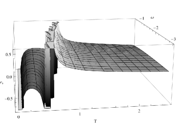
Figure 1: Variation of temperature with horizon radius for different values of $\omega$ with $\Lambda_{W}=0.0001$.

And for the region $r_{+}\textless\tilde{r}_{+}$, interestingly the temperature is found to be negative. The heat capacity of the black hole is given by

$$C = \frac{1}{128\pi^{3}r_{+}^{4}((\Lambda_{W}-\omega)r_{+}^{2}-1)^{3}}[(\Lambda_{W}r_{+}^{2}-1)^{3}(9\Lambda_{W}^{2}r_{+}^{4}-1)$$ (16)

$$+ 3r_{+}^{2}(1+\Lambda_{W}r_{+}^{2}(8-6\Lambda_{W}r_{+}^{2}-3\Lambda_{W}^{3}r_{+}^{6}))\omega$$

$$- 12r_{+}^{4}(1+\Lambda_{W}r_{+}^{2})\omega^{2}+4r_{+}^{6}\omega^{3}].$$

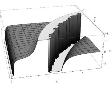
Figure 2: Variation of specific heat with horizon radius for different values of $\omega$ with $\Lambda_{W}=0.0001$.

In fig.2, variation of heat capacity with respect to the black hole horizon $r_{+}$ for different values of coupling parameters are plotted. From this figure we can see that specific heat undergoes a transition from negative values to positive values or in other words black hole changes from a thermodynamically unstable state to a thermodynamically stable state. By looking and comparing the two figures, fig.1 and fig.2, we can straightaway say that in the region where temperature shows the anomalous behaviour due to its negative values, the black hole is found to be thermodynamically unstable as its heat capacity is negative. Now for a Schwarzschild-dS black hole, from (12) we can write

$$f=1-\frac{\Lambda_{W}}{2}r^{2}-\frac{2M}{r}.$$

The event horizon is defined by $f(r_{+})=0$,

$$r_{+}-\frac{\Lambda_{W}}{2}r^{3}_{+}-2M=0.$$ (17)

So we can write the mass as,

$$M=\frac{r_{+}}{2}-\Lambda_{W}r_{+}^{3}.$$ (18)

Using the Bekenstein-Hawking area law,

$$S=\frac{A}{4}=\pi r_{+}^{2},$$ (19)

we can rewrite the mass-horizon relation (18) as,

$$M=\frac{1}{2}\sqrt{\frac{S}{\pi}}-\Lambda_{W}\left(\frac{S}{\pi}\right)^{3/2}.$$ (20)

Using the definition of temperature as $T=\left(\frac{\partial M}{\partial S}\right)$ and that of heat capacity as $C=T\left(\frac{\partial S}{\partial T}\right)$, we can arrive at

$$T=\frac{1}{4\sqrt{\pi S}}-\frac{3\Lambda_{W}\sqrt{S}}{2\pi^{3/2}},$$ (21)

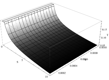
Figure 3: Variation of temperature with entropy for SdS black hole.

and

$$C=\frac{\pi^{2}}{3\Lambda_{W}\pi+18\Lambda_{W}^{2}S}-\frac{3\Lambda_{W}\sqrt{S}}{2\pi^{3/2}}-\frac{\pi}{3\Lambda_{W}}.$$ (22)

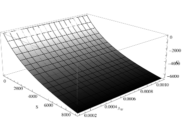
Figure 4: Variation of specific heat with entropy for SdS black hole.

Variation of temperature with respect to entropy is plotted in fig.3 while in fig.4 the variation of heat capacity with entropy is plotted. From fig.4 it is evident that Schwarzschild-dS black hole is thermodynamically unstable for all range of entropy values.

Now let us investigate peculiar behavior of Park black hole. As explained in Park , for the black hole horizon to exist and curvature singularity at $r=0$ is not naked, one has to consider another condition which is given by,

$$M\leq\frac{(2\Lambda_{W}-\omega)}{4}r_{+}^{3}.$$ (23)

Or we can say that, $M\textless\frac{(2\Lambda_{W}-\omega)}{4}r_{+}^{3}$ for all $r_{+}$ except for $r_{+}=\tilde{r}_{+}$. And at this point mass of the black hole meets the upper bound.

Now let us investigate the thermodynamics of the black hole which has a mass given by the upper mass bound value given in (23) i.e.,

$$M_{bound}=\frac{(2\Lambda_{W}-\omega)}{4}r_{+}^{3}.$$ (24)

Using Bekenstein-Hawking area law, we can rewrite (24) as

$$M_{bound}=\frac{(2\Lambda_{W}-\omega)}{4}\left(\frac{S}{\pi}\right)^{3/2}.$$ (25)

From the usual definition of temperature and that of heat capacity, we can arrive at

$$T=\frac{3(2\Lambda_{W}-\omega)\sqrt{S}}{8\pi^{3/2}},$$ (26)

and

$$C=2~{}S.$$ (27)

Since the heat capacity is positive, the black hole having a mass given by (24) is thermodynamically stable. From this fact we can say that the occurrence of infinite discontinuity as well as negative temperature must be due to the existence of a restriction given by (23) for the mass parameter.

4 Quasinormal modes of Park black hole

In this part of our work, our main aim is to study the quasinormal modes of massless scalar field of Park black hole in Hořava gravity. The Klein-Gordon equation for a massless scalar field in this space time is given by

$$\frac{1}{\sqrt{-g}}\partial_{\mu}\left(\sqrt{-g}g^{\mu\nu}\partial_{\nu}\right)\Phi=0.$$ (28)

Separating the scalar field in to spherical harmonics,

$$\Phi=\frac{1}{r}\Psi(r)Y(\theta,\phi)e^{-i\omega t}$$ (29)

and using the tortoise coordinate defined by $dr_{*}=\frac{1}{f}dr$, one can obtain the radial equation,

$$\frac{d^{2}\Psi(r)}{dr_{*}^{2}}+\left[\omega^{2}-V(r)\right]\Psi(r)=0,$$ (30)

in which the effective potential $V(r)$ is given by,

$$V(r)=f(r)\left[\frac{l(l+1)}{r}+\frac{1}{r}\frac{\partial f(r)}{\partial r}\right],$$ (31)

where (11) gives the $f(r)$.

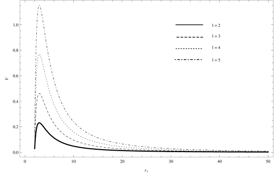
Figure 5: Variation of effective potential with horizon radius for different $l$ values.

The behaviour of effective potential for different values of angular quantum number $l$ is plotted in fig.5. From this figure we can say that as the $l$ value increases the potential barrier also get increased. Now we are evaluating the quasinormal frequencies of the scalar field around Park black hole using the third-order WKB approximation Schutz ; Iyerwill ; Iyer . The formula for the complex quasinormal frequencies $\omega_{QNM}$ in this approximation is given by

$$\omega_{QNM}^{2}=\left[V_{0}+(-2V_{0}^{{}^{\prime\prime}})^{1/2}\Lambda\right]-i(n+\frac{1}{2})(-2V_{0}^{{}^{\prime\prime}})^{1/2}(1+\Omega),$$ (32)

where

$$\Lambda = \frac{1}{(-2V^{{}^{\prime\prime}}_{0})^{1/2}}\Bigg{\{}\frac{1}{8}\left(\frac{V^{(4)}_{0}}{V^{{}^{\prime\prime}}_{0}}\right)\left(\frac{1}{4}+\alpha^{2}\right)$$ (33)

$$- \frac{1}{288}\left(\frac{V^{{}^{\prime\prime\prime}}_{0}}{V^{{}^{\prime\prime}}_{0}}\right)^{2}(7+60\alpha^{2})\Bigg{\}},$$

$$\Omega = \frac{1}{(-2V^{{}^{\prime\prime}}_{0})}\Bigg{\{}\frac{5}{6912}\left(\frac{V^{{}^{\prime\prime\prime}}_{0}}{V^{{}^{\prime\prime}}_{0}}\right)^{4}(77+188\alpha^{2})\frac{1}{384}\left(\frac{V^{{}^{\prime\prime\prime 2}}_{0}V^{(4)}_{0}}{V^{{}^{\prime\prime 3}}_{0}}\right)$$ (34)

$$(51+100\alpha^{2})+\frac{1}{2304}\left(\frac{V^{(4)}_{0}}{V^{{}^{\prime\prime}}_{0}}\right)^{2}(67+68\alpha^{2})$$

$$+ \frac{1}{288}\left(\frac{V^{{}^{\prime\prime\prime}}_{0}V^{(5)}_{0}}{V^{{}^{\prime\prime 2}}_{0}}\right)(19+28\alpha^{2})-\frac{1}{288}\left(\frac{V^{(6)}_{0}}{V^{{}^{\prime\prime}}_{0}}\right)(5+4\alpha^{2})\Bigg{\}}$$

and

$$\alpha=n+\frac{1}{2},~{}~{}~{}~{}~{}~{}~{}~{}~{}~{}~{}~{}~{}~{}~{}~{}~{}~{}~{}~{}V^{(s)}_{0}=\frac{d^{s}V}{dr^{s}_{*}}\bigg{|}_{\;r_{*}=r_{*}(r_{p})}$$ (35)

where $n$ is the overtone and $r_{p}$ is the value of polar coordinate $r$ corresponding to the peak value of effective potential $V(r)$ given in (31). Substituting the effective potential (31) in to the above formula, we can obtain the quasinormal frequencies of scalar perturbation for the Park black hole.

Table 1: The fundamental $(n=0)$ quasinormal frequencies of scalar filed in the Hořava de Sitter black hole for $l=1,2,3$ with $\Lambda_{W}=0.0001$

$\omega$	$\omega_{QNM}(l=1)$	$\omega_{QNM}(l=2)$	$\omega_{QNM}(l=3)$
-0.5	0.2916911–0.0981963i	0.4841694-0.0.096997150i	0.676545-0.09670374i
-1.0	0.2914027-0.09809888i	0.4836904-0.09690105i	0.67587629-0.096607976
-1.5	0.2913065-0.09806638i	0.48353071-0.09686899i	0.67565299-0.096576033i
-2.0	0.2912584-0.09805013i	0.48345081-0.09685296i	0.675541320-0.096560057i
-2.5	0.2912296-0.09804038i	0.48340280-0.09684334i	0.675474301-0.096550470i
-3.0	0.2912103-0.09803388i	0.48337089-0.09683693i	0.67542962-0.0965440780i

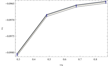
Figure 6: Massless scalar field QNMs of Park black hole for different values of $l$

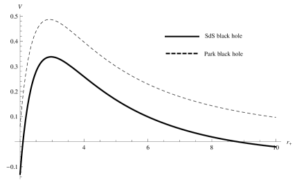
Figure 7: Variation of effective potential of SdS and Park black hole with horizon radius for a $l=3$.

The quasinormal frequencies are shown in Table.1. Fig.6 shows that the real and imaginary parts of the quasinormal frequencies changes slowly as the the parameter $\omega$ changes for fixed value of $\Lambda_{W}$. From Table.1, we can find that all frequencies have negative imaginary parts, which means that the black hole is stable against these perturbations.

Let us now consider the Schwarzchild-de Sitter case. In fig.7 we have plotted the effective potential for the Schwarzchild-de Sitter case along with the Park black hole case for a particular $l$ value. And from this figure we can see that the behaviour is almost the same. Applying the third-order WKB approximation method to evaluate the fundamental quasinormal modes and from the obtained quasinormal mode frequencies of SdS black hole and Park black hole, we can compare them. In fig.8 we have plotted the fundamental quasinormal mode frequencies for fixed values of $\Lambda_{W}$ and $\omega$ for these two black holes. From this it is evident that, both black holes show similar behaviour against these massless scalar perturbations. So as in the case of Park black hole, SdS black hole are also stable against these perturbations.

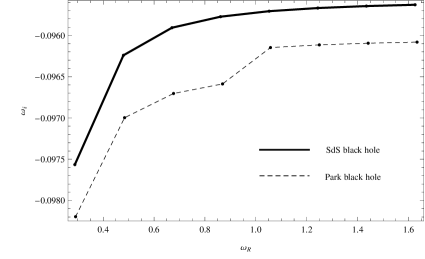
Figure 8: Massless scalar field QNMs of SdS and Park black holes for $l=3$.

5 Discussion and conclusion

In this paper we have investigated the quasinormal modes of the massless scalar field of Park black hole. QNMs are studied using the third-order WKB approximation method. We have found that the frequencies all have negative imaginary parts. Hence the Park black hole is stable against these perturbations. These results are compared with those of Schwarzschild-de Sitter case and find that they have almost the same behavior. We have also studied the thermodynamic aspects of Park black hole and find that it shows negative values as well as infinite discontinuity in temperature. This may be due to the existence of an upper bound of the mass parameter. In addition to this we have studied the thermodynamic properties of Park black hole which has a mass equal to the upper bound value of the mass parameter and found that these black holes are thermodynamically stable. When we study the perturbative effects on Park and SdS black hole, there is an agreement between them up to some numerical factor corrections, while they have entirely different thermodynamic behaviors.

References

- (1) Bardeen J. M., Carter. B., Hawking. S. W., Commun. Math. Phys., 31 (1973) 161.
- (2) Bekenstein J. D., Phys. Rev. D., 7 (1973) 2333.
- (3) Hawking S. W., Nature., 248 (1974) 30.
- (4) Hawking S. W., Commun. Math. Phys., 43 (1975) 43.
- (5) Perlmutter. S., et al., Astrophys. J., 483 (1997) 565.
- (6) Caldwell. R. R., Dave. R., Steinhardt. P. J., Phys. Rev. Lett., 80 (1998) 1582.
- (7) Garnavich. P. M., et al., Astrophys. J., 509 (1998) 74.
- (8) Maldacena. J. M., Adv. Theor. Math. Phys., 2 (1998) 231
- (9) Witten. E., hep-th/0106109.
- (10) Strominger. A., JHEP., 0111 (2001) 0341.
- (11) Strominger2. A., JHEP., 0111 (2001) 0491.
- (12) Hořava P., Phys. Rev. D, 79 (2009) 084008.
- (13) Hořava P., JHEP, 03 (2009) 020.
- (14) Hořava P., Phys. Rev. Lett., 102 (2009) 161301.
- (15) Lu H., Mei J, Pope C. N., Phys. Rev. Lett., 103 (2009) 091301.
- (16) Cai R. G., Cao L. M, Ohta N., Phys. Rev. D, 81 (2009) 024003.
- (17) Kehagias A, Sfetsos K., Phys. Lett. B, 678 (2009) 123.
- (18) Nastase. H., Phys. Lett. B, 67 (2009) 123.
- (19) Kiritsis E, Kofinas G., Nucl. Phys. B, 821 (2009) 467.
- (20) Calcagni G., JHEP, 09 (2009) 112.
- (21) Park M. i., JCAP, 01 (2010) 001.
- (22) Wei S. W, Liu Y. X, Guo H., EPL, 99 (2012) 20004.
- (23) Myung Y. S., Phys. Lett. B. 684 (2010) 158.
- (24) Myung Y. S., Phys. Lett. B. 678 (2009) 127.
- (25) Myung Y. S, Kim Y. W., Eur. Phys. J. C. 68 (2010) 265.
- (26) Nijo Varghese, V. C. Kuriakose., Mod. Phys. Lett. A, 26 (2011) 1645.
- (27) Nijo Varghese, V. C. Kuriakose., Gen. Relativ. Gravit., 43 (2011) 2755.
- (28) Jishnu Suresh, V. C. Kuriakose., Gen. Relativ. Gravit., 45 (2013) 1877.
- (29) Park M. i., JHEP, 0909 (2009) 123.
- (30) Vishveshwara. C. V., Nature., 227 (1970) 936.
- (31) Press. W. H., Astrophys. J., 170 (1971) 105.
- (32) Simone. L. E., Will. C. M., Classical Quant. Grav., 9 (1992) 963.
- (33) Konoplya. R. A., Phys. Lett. B., 550 (2002) 117.
- (34) Burko. R. A., Khanna. G., Phys. Rev. D., 70 (2004) 044018.
- (35) Hod. S., Phys. Rev. D., 84 (2011) 044046.
- (36) Chandrasekhar. S., Detweiler. S. L., P. Roy. Soc. A-Math. Phys., 344 (1975) 441.
- (37) Regge. T., Wheeler. J. A., Phys. Rev., 108 (1999) 1063.
- (38) Horowitz. G. T., Hubeny. V. E., Phys. Rev. D., 62 (2000) 024027.
- (39) Wang. B., et al., Phys. Rev. D., 70 (2004) 064025.
- (40) Hod. S., Phys. Rev. Lett., 81 (1998) 4293.
- (41) Dreyer. O., Phys. Rev. Lett., 90 (2003) 081301.
- (42) Iyer. S., Phys. Rev. D., 35 (1987) 3632.
- (43) Iyer. S, Will. C. M., Phys. Rev. D., 35 (1987) 3621.
- (44) Schutz. B. F, Will. C. M., Astrophys. J. Lett. Ed. 291 (1985) 33.
- (45) Konoplya. R. A., Phys. Rev. D., 68 (2003) 024018.