NIKHEF 2013-033

DAMTP-2013-61

Quantum corrections in Higgs inflation:
the real scalar case

Damien P. George^1,2, Sander Mooij^3,4 and Marieke Postma³

¹ Department of Applied Mathematics and Theoretical Physics,
Centre for Mathematical Sciences, University of Cambridge,
Wilberforce Road, Cambridge CB3 0WA, United Kingdom

² Cavendish Laboratory, University of Cambridge,
JJ Thomson Avenue, Cambridge CB3 0HE, United Kingdom

³ Nikhef,
Science Park 105,
1098 XG Amsterdam, The Netherlands

⁴ FCFM, Universidad de Chile,
Blanco Encalada 2008,
Santiago, Chile

ABSTRACT

We present a critical discussion of quantum corrections, renormalisation, and the computation of the beta functions and the effective potential in Higgs inflation. In contrast with claims in the literature, we find no evidence for a disagreement between the Jordan and Einstein frames, even at the quantum level. For clarity of discussion we concentrate on the case of a real scalar Higgs. We first review the classical calculation and then discuss the back reaction of gravity. We compute the beta functions for the Higgs quartic coupling and non-minimal coupling constant. Here, the mid-field regime is non-renormalisable, but we are able to give an upper bound on the 1-loop corrections to the effective potential. We show that, in computing the effective potential, the Jordan and Einstein frames are compatible if all mass scales are transformed between the two frames. As such, it is consistent to take a constant cutoff in either the Jordan or Einstein frame, and both prescriptions yield the same result for the effective potential. Our results are extended to the case of a complex scalar Higgs.

1 Introduction

In the paradigm of Higgs inflation the standard model (SM) Higgs doublet plays the role of the inflaton, and provides an almost-constant de Sitter vacuum energy to exponentially expand the universe during its initial stages [1, 2]. The model introduces a single new term to the standard model with gravity, to couple the Higgs doublet $\Phi$ to the Ricci scalar, $\xi R\Phi^{\dagger}\Phi$ [3, 4]. The associated dimensionless coupling constant $\xi$ must necessarily be large, $\xi\sim 2\times 10^{4}$ to give slow roll inflation in agreement with data from the cosmic microwave background (CMB). The classical analysis of Higgs inflation is well understood: one transforms to the Einstein frame to make the gravity sector canonical, redefines the Higgs degree of freedom (in unitary gauge) to obtain a canonical kinetic term, and uses the resulting potential to compute slow roll parameters in the usual way. This gives a connection between the quartic coupling in the Higgs potential and the new non-minimal coupling, and parameters of the CMB, $n_{s}$ and $r$.

Higgs inflation is a theory spanning many orders of magnitude in energy. The couplings in the SM are measured by collider experiments at energies around the electroweak scale, whilst inflation and its observables are defined at the inflationary scale, 13 orders of magnitude higher. This disparity of scales means that the leading logarithmic corrections due to quantum loops will be large, or, equivalently, that the running of the couplings is significant from the electroweak to the inflationary scale. It is therefore important to consider quantum effects in Higgs inflation, but in doing so many problems arise, both conceptual and technical [5, 6, 7, 8, 9, 10, 11, 12, 13, 14].

The main quantity of interest is the loop-corrected effective potential of the Higgs/inflaton. As previously mentioned, knowledge of the potential allows one to compute slow roll parameters, and incorporating loop-corrections and running of the couplings allows one to obtain a more accurate answer. The different degrees of freedom in the SM all provide competing corrections, along with corrections due to Hubble expansion; also there is the important fact that the Higgs quartic coupling runs very close to zero. The transformation of the theory from the original Jordan frame where the theory is defined, to the Einstein frame with canonical gravity, leads to additional issues depending on which frame the quantisation is performed in. Quantising in the Jordan frame with gravity a non-dynamical background leads to incorrect beta functions for the running couplings, unlike in the Einstein frame where non-dynamical gravity introduces only a small error. Renormalising the theory in either frame with a constant UV cutoff can lead to different results if not done correctly. Finally, the model itself is inherently non-renormalisable, and so at certain points in field space it seems impossible to compute loop corrections to the potential.

For Higgs inflation as a theory to make accurate predictions it is crucial to sort out all of the above-mentioned issues in a consistent and rigorous way. It is the aim of this paper to address these issues and give a conservative set of answers and associated formulae. We will discuss the following points.

• At the classical level, the conformal transformation relating the Jordan and Einstein frames is just a redefinition of the fields, and the two frames are physically equivalent. The two- and three-point functions of the perturbations during inflation are the same in both frames [15, 16, 17, 18, 19, 20]. We shall demonstrate that this equivalence also holds for the 1-loop effective potential, and, derived from that, for the beta functions. The Jordan or Einstein frame (or any other frame) is not fundamentally better, it is just easier in some frames to compute certain quantities.

• In the literature it is argued that calculating the effective potential in the Jordan frame gives a field-dependent cutoff in the Einstein frame and vice versa [6, 7, 10, 12, 14]. Moreover, these two prescriptions are then claimed to lead to two different effective potentials. We show explicitly that in both frames the dependence on the cutoff can safely be eliminated and that both frames give the same result. Therefore, the theory does not depend on the choice of the cutoff, or on the UV completion.

• One item that is expressed differently between the two frames is the adiabatic scalar degree of freedom. Indeed, it is a different mixture of the Higgs field and the scalar degree of freedom in the metric the Jordan frame than in the Einstein frame. If one treats gravity as a classical background and only quantises the Higgs field, this thus amounts to different approximations. The approximation is fine for the Einstein frame, where the error made is of the order of the slow roll parameter $\epsilon$ and therefore subleading. However, we will claim that in the Jordan frame this approximation is not at all valid. As a result, the renormalisation group equations (RGEs) thus found in the Jordan frame [6, 21, 22, 23, 10, 12, 13] are incorrect. Note in this respect that also the RGE for the non-minimal couplings used in [9] treats gravity classically in the Jordan frame.

• The theory is renormalisable in the small field regime (in the usual sense of low energy effective field theories) and in the large field regime (thanks to an approximate shift symmetry [8, 27]). In the mid-field regime the theory is most likely non-renormalisable, but we are still able to compute the leading order contribution to the RGEs in this range, being as conservative as possible. Thus, the potentially infinite number of counter terms that need to be introduced to properly renormalise the theory are parametrically suppressed, and we can still make predictions.

• The Higgs doublet has four scalar degrees of freedom, and the non-minimal coupling to gravity means that these scalars are inherently mixed (their quadratic terms in the action are not simultaneously diagonalisable [32]). We show how to include such degrees of freedom in quantum loops by diagonalising the mass matrix, for a fixed point in field space, to find the physical masses for the 1-loop contribution to the effective potential. Both the contribution of the Higgs and the (massive) Goldstone bosons are suppressed during inflation. This is in contrast with the claims made in Refs. [12, 13, 14] that only the Higgs field is suppressed.

• Due to the large non-minimal coupling $\xi$, unitarity of $\text{SU}(2)$ gauge boson scattering is lost below the inflationary scale in the small and mid-field regimes [24, 25, 26]. The unitary bound is field dependent, and it has been shown that in all three regimes the typical energy scales in Higgs inflation are parametrically lower than the scale of unitarity violation [8, 27]. That may already solve the problem of non-unitarity of Higgs inflation, but new physics still seems required to restore unitarity in the SM vacuum. However, we think that the situation is actually even better. We shall briefly comment on the possibility that this new physics necessarily appears only at Planck-scale energies. This gives further hope that the predictions of Higgs inflation can be trusted.

As the issues involved are largely conceptual, we start with the simplest setting, that of a real scalar field with a non-minimal coupling, and extend to a complex field in the latter sections of the paper. Since there is no gauge sector, the anomalous dimension of the Higgs vanishes and we also do not have gauge or (fermionic) Yukawa couplings to deal with. Only the correction to the effective potential needs to be calculated. The 1-loop effective potential can be expressed in terms of the masses of the fields, i.e. only depends on the action at the quadratic level, and is not hampered by the complicated non-minimal kinetic terms. Since the Higgs is light during inflation, its contribution should be calculated in FLRW; in other regimes a Minkowski approximation suffices. Even with these simplifications it is still possible to discuss and address all of the above-mentioned issues. In a follow up paper we aim to build upon the results obtained here and look at the full standard model.

It is important to note that a Higgs mass $m_{h}=125~{}\text{GeV}$, compatible with the measurements by ATLAS and CMS [37, 38], leads to the Higgs quartic coupling $\lambda$ running negative at energies below the inflationary scale [39, 40]. This is for central values of the top mass and strong coupling, and can be avoided, albeit marginally, by taking $m_{t}\sim 171~{}\text{GeV}$, $3\sigma$ lower than the central value [41]. One could also extend the minimal Higgs inflation model to include additional particles that modify the running of $\lambda$ [42, 43]. Whatever the specifics, the results presented here can be applied to such a model, and can also be applied more generally to models of inflation where the inflaton scalar is not the Higgs doublet, but is still non-minimally coupled to the Ricci scalar. We do assume, though, that the non-minimal coupling is large $\xi\gg 1$, and can be used as an expansion parameter.

The paper is organised as follows. We begin in Sec. 2 by reviewing the well established classical calculation, and discuss the back reaction from gravity. In Sec. 3 we find the beta functions for the quartic coupling and non-minimal coupling $\xi$, including a conservative bound on the running of the couplings in the non-renormalisable mid-field regime. In Sec. 4 we discuss the equivalence of the Jordan and Einstein frames when computing the effective potential. We show how the Jordan and Einstein frames should give a result independent of which frame the cutoff is chosen to be constant in. In addition, we argue that in the Einstein frame gravity can be treated as a non-dynamical background and only introduces a small error, in contrast with the Jordan frame. Our results are extended to a complex scalar Higgs in Sec. 5, and we make some brief remarks in Sec. 6 on the unitarity bound. Finally, Sec. 7 compares our results with the literature and draws conclusions.

2 Higgs inflation, the classical background

Higgs inflation takes the SM Lagrangian with the Einstein-Hilbert term for gravity and adds a non-minimal coupling between the Higgs doublet $\Phi$ and the Ricci scalar $R$ [1, 2, 3, 4]. The Jordan frame is the frame in which the theory is defined, the Lagrangian being (with $+---$ metric signature)

$$\mathcal{L}_{J}=\sqrt{-g^{J}}\left[-\frac{1}{2}M_{\rm P}^{2}\left(1+\frac{2\xi\Phi^{\dagger}\Phi}{M_{\rm P}^{2}}\right)R[g^{J}]+\mathcal{L}_{\rm SM}\right].$$ (1)

A label $J$ denotes a Jordan frame quantity, $M_{\rm P}$ is the Planck mass and $\xi$ is the new dimensionless coupling. For the purposes of this paper we require only the Higgs sector, and so drop the gauge fields and fermions. Thus, the only relevant parts of the SM Lagrangian are the Higgs kinetic term and the Higgs potential

$$V_{J}=\lambda(\Phi^{\dagger}\Phi-v^{2}/2)^{2}.$$ (2)

The Einstein frame is obtained by redefining the metric degrees of freedom such that gravity is in its canonical Einstein-Hilbert form. As a result, the non-minimal coupling to gravity is removed and appears instead as non-canonical kinetic structure in the matter sector. The appropriate transformation is a conformal Weyl rescaling, made by $g_{\mu\nu}=\Omega^{2}g^{J}_{\mu\nu}$, with

$$\Omega^{2}=\left(1+\frac{2\xi\Phi^{\dagger}\Phi}{M_{\rm P}^{2}}\right).$$ (3)

The new Einstein-frame metric is $g_{\mu\nu}$, and the resulting Lagrangian is

$$\mathcal{L}_{E}=\sqrt{-g}\left[-\frac{1}{2}M_{\rm P}^{2}R[g]+\frac{1}{\Omega^{2}}(\partial_{\mu}\Phi)^{\dagger}(\partial^{\mu}\Phi)+\frac{3\xi^{2}}{M_{\rm P}^{2}\Omega^{4}}\partial_{\mu}(\Phi^{\dagger}\Phi)\partial^{\mu}(\Phi^{\dagger}\Phi)-\frac{V_{J}}{\Omega^{4}}\right].$$ (4)

We define the Einstein frame potential $V=V_{J}/\Omega^{4}$. The Higgs kinetic term is non-minimal and mixes the 4 degrees of freedom in the doublet. The model can be considered a non-linear sigma model with a non-trivial target/field space. Let $\chi_{i}$ run over all real fields in cartesian space, namely $\sqrt{2}\Phi^{\intercal}=(\chi_{1}+\mathrm{i}\chi_{2},\chi_{3}+\mathrm{i}\chi_{4})$; this generalises easily to other sized multiplets. Then the field-space metric in component form is $\gamma_{ij}$ defined by

$$\frac{\mathcal{L}_{E}}{\sqrt{-g}}\supset\frac{1}{2}\gamma_{ij}\partial\chi_{i}\partial\chi_{j}=\frac{1}{2}\left[\frac{\delta_{ij}}{\Omega^{2}}+\frac{6\xi^{2}}{M_{\rm P}^{2}\Omega^{4}}\chi_{i}\chi_{j}\right]\partial\chi_{i}\partial\chi_{j}.$$ (5)

The curvature on field space is non-zero, $R[\gamma_{ij}]\neq 0$, and hence there is no field redefinition among the set $\{\chi_{i}\}$ which diagonalises the kinetic terms [32]. This problem has a partial solution if one expands the fields around a fixed background, $\chi_{i}=\chi^{0}_{i}+\delta\chi_{i}$, and diagonalises the kinetic term for $\delta\chi_{i}$ at a specific point in field space defined by $\{\chi^{0}_{i}\}$. This is akin to the situation in general relativity where, if the space-time curvature is non-zero, one can go locally to a Minkowski frame, but not globally. Considering $\Phi$ a real scalar field with only 1 component this problem disappears, as the kinetic terms for a single degree of freedom can always be diagonalised.

For the classical analysis of Higgs inflation one considers only the background radial mode of $\Phi$, call it $\phi$, defined by $\phi^{2}=2|\Phi|^{2}$. This field can be canonically normalised via

$$\frac{1}{2}\gamma(\phi)(\partial\phi)^{2}=\frac{1}{2\Omega^{2}}\left(1+\frac{6\xi^{2}}{M_{\rm P}^{2}\Omega^{2}}\phi^{2}\right)(\partial\phi)^{2}=\frac{1}{2}(\partial h)^{2}.$$ (6)

The differential equation can be solved for $h$, but the solution is complicated and does not give much insight (it also cannot be inverted to get $\phi(h)$). Instead, we solve it in the three regimes — small field, mid field and large field — and then patch them together [8, 27]. The value of $\xi$ is large (as will be shown shortly) and its inverse is used to define the boundaries of the three regimes. From now we on we set $M_{\rm P}=1$.

1. Small field regime: $\phi<1/\xi$. Then $h^{\prime}(\phi)\sim 1$, and with the boundary condition $h(0)=0$ the solution is

   $$h=\phi.$$ (7)

   The effect of the non-minimal coupling is negligibly small.

2. Mid field regime: $1/\xi<\phi<1/\sqrt{\xi}$. Then $h^{\prime}(\phi)\sim\sqrt{6}\xi\phi$. Matching to the small field regime gives the boundary condition $h(1/\xi)=1/\xi$, and solution

   $$h=\sqrt{3/2}\xi\phi^{2}+(1-\sqrt{3/2})/\xi.$$ (8)

3. Large field regime: $\phi>1/\sqrt{\xi}$. Then $h^{\prime}(\phi)\sim\sqrt{6}/\phi$. The boundary condition is $h(1/\sqrt{\xi})=\sqrt{3/2}$, yielding the solution

   $$h=\sqrt{6}\ln(\phi\sqrt{\xi})+\sqrt{3/2}\qquad\Rightarrow\qquad\phi=\frac{1}{\sqrt{\xi}}{\rm e}^{(h-\sqrt{3/2})/\sqrt{6}}.$$ (9)

In the large field regime the potential can be expanded in

$$\delta\equiv\frac{1}{(\xi\phi^{2})}\ll 1.$$ (10)

Note that $\delta$ is independent of both $\xi$ and $\lambda$ when expressed in terms of the canonically normalised field $h$. Furthermore, neglecting the small mass term $v$, the potential only depends on the combination $\bar{\lambda}\equiv\lambda/\xi^{2}$. We expand all quantities to first order in $\delta$. This gives for the kinetic terms $\sqrt{\gamma}=\sqrt{6}/\phi(1-\delta)+\mathcal{O}(\delta^{2})$. Here terms $1/\xi\ll 1$ are neglected, thus the result is only valid for large non-minimal coupling. The exponential solution for $h$ given in (9) is only valid to lowest order. To find the derivatives of the potential we use $\sqrt{\gamma}V_{h}=V_{\phi}$, and similar for higher derivatives; this takes first order corrections into account. Up to $\mathcal{O}(\delta^{2})$ we find

$$V=\frac{\bar{\lambda}}{4}\left(1-2\delta\right),\quad V_{h}=\frac{\bar{\lambda}\delta}{\sqrt{6}}(1-2\delta),\quad V_{hh}=\frac{-\bar{\lambda}\delta}{3}(1-3\delta),\quad V_{hhh}=\frac{2\bar{\lambda}\delta}{3\sqrt{6}}(1-5\delta).$$ (11)

Using the standard expressions for the slow roll parameters, $\epsilon=(V_{h}/V)^{2}/2$ and $\eta=V_{hh}/V$, we obtain

$$\epsilon=\frac{4}{3}\delta^{2},\quad\eta=-\frac{4}{3}(\delta-\delta^{2}).$$ (12)

Inflation ends for $\epsilon\approx 1$ which gives $\delta_{\rm end}\sim\sqrt{3/4}$. The number of e-folds is

$$N=\int{\rm d}h(2\epsilon)^{-1/2}=\int{\rm d}\phi\frac{V}{V_{\phi}}\left(\frac{\partial h}{\partial\phi}\right)^{2}\approx\frac{3}{4}\xi(\phi_{*}^{2}-\phi_{\rm end}^{2})\approx\frac{3}{4\delta_{*}}.$$ (13)

Setting $N\approx 60$, we find $\delta_{*}\sim 3/4N\approx 1/80$ when observable scales leave the horizon. The COBE normalisation gives

$$\left(\frac{V}{\epsilon}\right)_{*}=(0.027)^{4}\qquad\Rightarrow\qquad\bar{\lambda}=4\times 10^{-10}\qquad\Rightarrow\qquad\xi/\sqrt{\lambda}=5\times 10^{4}.$$ (14)

Since $\lambda\sim 0.1$ in the SM we require $\xi$ of order $2\times 10^{4}$ to agree with the data. The predictions for the spectral index and tensor-to-scalar ratio are

$$n_{s}=1+2\eta-6\epsilon\approx 1-\frac{8}{3}\delta_{*}-\frac{16}{3}\delta_{*}^{2}\approx 0.966,\qquad r=16\epsilon=8\delta_{*}^{2}=0.0032.$$ (15)

These are within current $1\sigma$ bounds from Planck [33].

2.1 Back reaction of gravity

The results used above for the perturbation spectrum take into account the back reaction of gravity, that is the mixing between the Higgs field and scalar degree of freedom in the metric. Only during inflation these gravity corrections are important, i.e. in the large field regime. In this subsection we quickly review the approximation that takes gravity as a classical background. As we will discuss later, for the quantum corrections calculated in the Einstein frame this is a good lowest order approximation, because of a hierarchy in the slow roll parameters $\epsilon\ll\eta$; however, for the calculation in the Jordan frame, it fails.

Consider a canonical real scalar during inflation, and expand it around a classical background $\sqrt{2}\Phi(\vec{x},t)=\phi(t)+\delta\phi(\vec{x},t)$. We work in conformal coordinates ($\tau$ is conformal time) using an FLRW metric with scale factor $a$, and rescale the fields $\hat{\phi}=a\phi$ etc. Neglecting the back reaction the quadratic action for the scalar perturbations is

$$S^{(\text{quad})}=-\frac{1}{2}\int{\rm d}\tau{\rm d}^{3}x\delta\hat{\phi}\left(\partial^{2}+\hat{m}_{\delta\phi}^{2}\right)\delta\hat{\phi},$$ (16)

with effective “conformal” mass $\hat{m}^{2}_{\delta\phi}=a^{2}m_{\delta\phi}^{2}$ where

$$m_{\delta\phi}^{2}=\left[V_{\phi\phi}-(\dot{H}+2H^{2})\right]=-H^{2}\left(2-3\eta-\epsilon_{H}\right).$$ (17)

In this section we use the slow roll approximation which implies $\epsilon\approx\epsilon_{H}$ (with $\epsilon\equiv 1/2(V_{h}/V)^{2}$ and $\epsilon_{H}\equiv-\dot{H}/H^{2}$) and $\eta\approx\eta_{H}$ (with $\eta\equiv V_{hh}/V$ and $\eta_{H}\equiv\ddot{\phi}/(H\dot{\phi})+\epsilon_{H}$). Furthermore we use the third slow roll parameter $\qquad\xi_{(2)}=-\dddot{\phi}/(H^{2}\dot{\phi})$. One can now quantise the above action for the harmonic oscillator with a time-dependent mass, and derive the perturbation spectrum.

We now contrast this with the action when the back reaction of gravity is included. The effective scalar degree of freedom during inflation is a mixture of a metric degree of freedom and the Higgs field, which can be expressed in gauge invariant form via the Sasaki-Mukhanov variable [44, 45, 46]

$$v=a\left(\delta\phi+\frac{\dot{\phi}}{H}\psi\right).$$ (18)

In flat gauge, we can identify the Sasaki-Mukhanov variable with the Higgs field. The action for the Sasaki-Mukhanov variable is again that of a canonically normalised and time-dependent harmonic oscillator (16), but now with effective mass:

$$m^{2}_{v} =-\frac{z^{\prime\prime}}{z}=-H^{2}\left(2+5\epsilon_{H}-3\eta_{H}+(6\epsilon_{H}^{2}-4\epsilon_{H}\eta_{H}-\xi_{(2)})\right),$$

$$\to-H^{2}\left(2-3\eta+5\epsilon+\mathcal{O}(\epsilon^{2},\eta^{2})\right).$$ (19)

This is to be compared with (17), for the case of a probe field. The difference between including and neglecting gravity’s back reaction is of order $\epsilon$. For Higgs inflation $\epsilon\sim\delta^{2}$ and $\eta\sim\delta$, with the expansion parameter $\delta$ defined in (10). To lowest order in $\delta$ we can therefore ignore the back reaction. As discussed in Sec. 4.2, this is not the case if inflation is analysed in the Jordan frame.

3 Calculation of the beta functions

Our aim in this section is to compute the beta functions for the couplings $\lambda$ and $\xi$. We ignore the parameter $v$ in the Higgs potential as it is negligibly small and plays little role at energies above the electroweak scale. The beta function, and hence the RGEs, can be derived from the UV divergent part of the effective potential, and is the approach we adopt here. A previous set of works [28, 29] shows how one can calculate the effective potential by keeping the classical Higgs field $\phi_{\text{cl}}$ constant, and time-dependence, if necessary, can be incorporated by simply setting $\phi_{\text{cl}}\to\phi_{\text{cl}}(t)$. The result is then the usual Coleman-Weinberg (CW) potential [36]. With the effective potential and RGEs at hand one can then construct the renormalisation group (RG) improved effective action (see e.g. [48]).

We perform the calculation in the Einstein frame, for two main reasons. First, most of our intuition and standard results are valid in this frame, where gravity is minimally coupled. In the Einstein frame there is a clear interpretation of mass scales, in contrast with the Jordan frame where field-dependent measuring sticks are used (due to a field-dependent Planck mass). Second, in the Einstein frame gravity can be treated as a classical background, as discussed later in Sec. 4.2, and we do not need to worry about a strong coupling between quantum degrees of freedom which correct the classical potential, and gravity perturbations.

Because the potential in the Einstein frame is non-renormalisable we split the running into the small, mid- and large field regimes and consider each regime as a separate effective field theory (EFT). As long as energies stay below the cutoff of the EFT we can renormalise the couplings and compute the beta functions in each regime, and patch them together to obtain a final answer.

The CW corrections to the potential depend on the masses of the fields running in the loop; in our case we have only the Higgs. As computed in Ref. [29], treating gravity as a classical background, the FLRW space-time corrects the masses in the loop by an amount proportional to $\dot{H}+2H^{2}$. In Fig. 1 we plot the Hubble scale $H^{2}$ and Higgs mass squared, under the assumption that the Higgs field dominates the energy density (which is valid during inflation and gives only a negligible error afterwards). As can be seen, during inflation the Hubble scale dominates the Higgs mass and so we need to take the FLRW quantum corrections into account. After inflation these can be neglected and a Minkowski calculation suffices.

Our aim in computing the beta functions is to relate low and high scale observables by running the couplings in between the electroweak and inflationary scale. To that end we assume that the running is path independent, that is, independent of the precise details of how the inflaton (the Higgs in our case) rolled down the potential and the universe was reheated. As long as the time-evolution is (close to) adiabatic it should be safe to make such an assumption.

We use dimensional regularisation with MS-bar renormalisation prescription. We do not include the anomalous dimension, as it vanishes and so does not contribute to the running.

3.1 Higgs mass in the Einstein frame

For the loops, we need to compute the physical Higgs mass in the Einstein frame. With non-canonical kinetic terms, masses can be computed using the covariant generalisation of $m_{\phi}^{2}=\partial_{\phi}^{2}V$, namely

$$(m^{2})^{i}_{j}=\gamma^{ik}D_{k}D_{j}V(\phi)=\gamma^{ik}(\partial_{k}\partial_{j}V-\Gamma^{l}_{kj}\partial_{l}V),$$ (20)

with $\gamma_{ij}$ the field space metric, and $\Gamma^{i}_{jk}$ the associated connection coefficients. For now we take the Higgs as a real scalar (we treat the complex case in Sec. 5), which simplifies (20) and gives for the Higgs mass (using $\xi\gg 1$)

$$m_{h}^{2}=3\lambda\phi^{2}\frac{(1+4\xi^{2}\phi^{2}-4\xi^{3}\phi^{4})}{\Omega^{4}(1+6\xi^{2}\phi^{2})^{2}}\approx\{3\lambda\phi^{2},\;\frac{\lambda}{3\xi^{2}},\;-\frac{\lambda}{3\xi^{3}\phi^{2}}\},$$ (21)

where the second expressions are the leading terms in the three field regimes. The Higgs mass squared is negative during inflation. The potential is convex, leading to a red tilted spectral index in excellent agreement with the data. (Note however that these masses are computed in a Minkowski background. In the large field regime we will have to take the expansion of the universe into account, which leads to extra FLRW-corrections.)

3.2 Small field regime

To obtain the dominant terms responsible for the running in the small field regime we expand the action in the small parameter $\delta\equiv\xi\phi\ll 1$. At lowest order the potential reduces to the familiar $\phi^{4}$ theory. Indeed, to lowest order the canonically renormalised field is $h=\phi$, and the classical potential is $V^{\text{cl}}=\lambda\phi^{4}/4$. The non-minimal coupling $\xi$ drops out completely. The CW correction to the potential is [36]

$$\delta V=\frac{1}{64\pi^{2}}\sum_{i}(-1)^{f_{i}}m_{i}^{4}\left[\ln\frac{m_{i}^{2}}{\mu^{2}}-c_{i}\right]$$ (22)

with $f_{i}=1(-1)$ for a boson (fermion), and $c_{i}=3/2$ for a fermion and scalar boson, and $c_{i}=5/6$ for a vector boson in the $\overline{\rm MS}$ scheme; $\mu$ is the renormalisation scale. For the Higgs field the effective mass in the small field regime is $m^{2}_{h}=3\lambda\phi^{2}$, see (21). The beta functions are found by demanding the full potential to be independent of the arbitrary renormalisation scale, $\mu({\rm d}V/{\rm d}\mu)=0$, giving

$$\beta_{\lambda}\partial_{\lambda}V^{\rm cl}=-\mu\partial_{\mu}\delta V,$$ (23)

with $\beta_{\lambda}\equiv\mu\partial_{\mu}\lambda$. This gives the standard result

$$\beta_{\lambda}=\frac{9}{8\pi^{2}}\lambda^{2}.$$ (24)

The theory is renormalisable in the usual EFT sense: higher order terms are irrelevant operators and can be neglected at low scales. However, we can improve the calculation by including the next order in $\delta$. This introduces the leading irrelevant operator in the tree-level potential and its coefficient includes the non-minimal coupling $\xi$, allowing us to compute the running of this coupling. To this next order we find $\phi=h-\xi^{2}h^{3}+\mathcal{O}(\delta^{4})$ and

$$V^{\text{cl}}=\frac{\lambda}{4}h^{4}-\lambda\xi^{2}h^{6}+\mathcal{O}(\delta^{4}).$$ (25)

The leading term that we have ignored in $V$ goes like $\delta^{4}h^{4}$, which is subdominant to the sextic term $\lambda\xi^{2}h^{6}\sim\delta^{2}h^{4}$. Using (25) we can calculate the effective Higgs mass and thus the CW potential. Neglecting $h^{8}$ terms in the 1-loop potential (higher order counter terms need to be introduced to absorb this divergence) we can derive the beta functions for $\lambda$ and $\xi$ from the quartic and sextic operators via

$$[\beta_{\lambda}\partial_{\lambda}+\beta_{\xi}\partial_{\xi}]V^{\text{cl}}=-\mu\partial_{\mu}\delta V$$ (26)

The beta function for the coupling is as before (24); in addition we find

$$\beta_{\xi}=\frac{9}{4\pi^{2}}\lambda\xi.$$ (27)

This result is only of theoretical importance, as the effect of $\xi$, even though the coupling is large, is too small at electroweak scales for it to be measurable. Putting back powers of $M_{\rm P}$ we see that the coefficient of the $h^{6}$ term in (25) is $-\lambda\xi^{2}/M_{\rm P}^{2}$, corresponding to a scale roughly $10^{15}$ GeV, and is thus not measurable by colliders in the foreseeable future. We cannot therefore probe the running of $\xi$ experimentally in the small field regime. On the other hand the coupling $\lambda$ can be be independently measured, through the $h^{4}$ operator. Our main point here is that although to lowest order $\xi$ drops out, it still runs in the small field regime. Indeed, the running is not suppressed by large scales and does not vanish in the small field regime.

3.3 Large field regime

We look next at the running in the large field regime, where the expansion parameter is $\delta\equiv 1/(\xi\phi^{2})\ll 1$. In the slow roll approximation the effective mass of the adiabatic mode which runs in the loop is, from (19), $m_{h}^{2}=-H^{2}(2-3\eta+5\epsilon)$.

For technical reasons it is easier to work at the level of the equation of motion, rather than of the effective action directly. We use flat gauge, where we can identify the Sasaki-Mukhanov variable with the Higgs field. The 1-loop corrected equation of motion for the canonically normalised field $h$ is (see Eq. (35) of Ref. [47])

$$0=\ddot{h}+3H\dot{h}+V_{h}+\left(\frac{1}{2}V_{hhh}+\frac{3}{4}\frac{\dot{h}}{H}H^{2}(3\eta-2\epsilon)\right)G_{h}(0),$$ (28)

with the equal-time propagator

$$G_{h}(0)=\frac{1}{16\pi^{2}}m_{h}^{2}\left(\ln\frac{m_{h}^{2}}{\mu^{2}}-\frac{3}{2}\right),$$ (29)

where $\mu$ is the renormalisation scale. As before we work with the coupling $\bar{\lambda}\equiv\lambda/\xi^{2}$; the classical potential is only a function of $\bar{\lambda}$, and thus so are the quantum corrections; see (11).

To find the beta functions we require the effective potential to be independent of the renormalisation scale. Working at the level of the equation of motion avoids having to integrate to get the action, and independence of $\mu$ implies

$$\beta_{\bar{\lambda}}\partial_{\bar{\lambda}}V_{h}^{\rm cl}=-\left(\frac{1}{2}V_{hhh}+\frac{3}{4}\frac{\dot{h}}{H}H^{2}(3\eta-2\epsilon)\right)\partial_{\ln\mu}G_{h}(0).$$ (30)

The last term in (28) and (30) comes from treating gravity dynamical, and is otherwise absent. This correction is subdominant in the expansion parameter $\delta$. Moreover, the correction to the mass (and thus the propagator) due to back reaction is order $\epsilon$, which is also negligible to lowest order (since $\eta\sim\delta$ and $\epsilon\sim\delta^{2}$).

To evaluate $\beta_{\bar{\lambda}}$ we eliminate the Hubble parameter in (30) using the background equations of motion $\dot{h}^{2}=2\epsilon H^{2}$ and $H^{2}=V(1+\epsilon/3)/3$, and thus $\dot{h}/H=-\sqrt{2\epsilon}$ (the minus sign because the field is rolling down). We then use (11, 12) to trade the potential and its derivatives, and the slow roll parameters, in terms of an expansion in $\delta$. This gives the 1-loop corrections to the equation of motion, and at lowest order in $\delta$ we find:

$$\beta_{\bar{\lambda}}=-\frac{\bar{\lambda}^{2}}{144\pi^{2}}+\mathcal{O}(\delta).$$ (31)

The minus sign comes about because $m_{h}^{2}$ is negative, while $V_{hhh}$ is positive (usually, for minimally coupled fields, one gets a factor $(\partial_{h_{0}}m^{2})m^{2}>0$, and the quartic coupling has a positive-sign beta function). Note in this respect that when Hubble corrections dominate the mass term, the expression $\delta V\sim m^{4}\ln\mu$ is no longer a good approximation. The Hubble corrections to the mass come from the kinetic terms (they are derivatives of the scale factor) and only show up in the quadratic action. The cubic action remains unaltered in an expanding universe. Hence, when calculating the tadpole diagram, the result is as in (28).

To get the lowest order result in slow roll parameters (more precisely, in $\delta$) one can treat gravity as a classical background, since, as shown in Sec. 2.1, in the Einstein frame dynamical gravity introduces corrections of order $\delta^{2}$. Higher order corrections should only give consistency conditions. If the theory is renormalisable, and so only a finite number of counter terms are needed to absorb all divergencies, the divergencies found at next order in $\delta$ should automatically be absorbed. To check this, we also calculated the beta function at next order, which includes the back reaction from gravity. We find indeed a consistent result, specifically, (31) is correct to $\mathcal{O}(\delta^{2})$. As discussed in [8] the renormalisability of the theory can be understood in that the potential in the large field regime asymptotes to a constant, and has an approximate shift symmetry. This means that quantum corrections should also respect the approximate shift symmetry, and thus be of the same form. This assures that they can be absorbed in the counter terms of the classical potential.

To compare the large-field beta function with the beta functions calculated in the small field regime, we find an expression for $\beta_{\bar{\lambda}}$ valid for small field:

$$\beta^{\text{small}}_{\bar{\lambda}}=-\frac{27}{8\pi^{2}}\bar{\lambda}^{2}\xi^{2}.$$ (32)

Note that the numerical coefficient in (31) is much smaller than in the small field regime, and it is also down by the large factor $\xi^{2}$. The running is thus relatively slow in the large field regime, which is as expected since the potential asymptotes to a constant there.

3.4 Mid-field regime

The issue of renormalisability becomes acute in the mid-field regime. In the small field regime renormalisability was assured because higher order operators are irrelevant in the IR limit, whereas in the large field regime the shift symmetry came to the rescue. In the mid field regime we have neither, and as a consequence the best we can do (without specifying any UV completion of the model) is to put a bound on bound on how big the corrections will be.

In the mid field regime the expansion parameters are $x\equiv\xi\phi^{2}\ll 1$ and $y\equiv\xi^{2}\phi^{2}\gg 1$, and we expand in both (taking them both equally small, i.e. write $x\to\delta x$ and $1/y\to\delta/y$ and expand in $\delta$). This is only a good approximation in the middle of this regime, where both expansion parameters are order $0.1$. Equivalently, one can take the expansion parameter to be $\delta=1/\sqrt{\xi}\ll 1$, so that $\xi=\delta^{-2}\tilde{\xi}$ and $\phi=\delta^{3/2}\tilde{\phi}$, where $\tilde{\xi}$ and $\tilde{\phi}$ are order 1 quantities. Then the boundaries of the mid-field regime are $x=\delta\tilde{\xi}\tilde{\phi}^{2}$ and $1/y=\delta/\tilde{\xi}^{2}\tilde{\phi}^{2}$, and as $\delta\to 0$ these bounds approach $(0,\infty)$.

Since the Hubble parameter drops fast below the Higgs mass in this regime (see Fig. 1), we can neglect gravity corrections and do a Minkowski calculation.

Expanding in $\delta$ the Einstein frame potential and the effective Higgs mass (21) yields

$$V =\frac{\lambda}{4}\delta^{6}\phi^{4}\left(1-2\delta\xi\phi^{2}+3\delta^{2}\xi^{2}\phi^{4}-4\delta^{3}\xi^{3}\phi^{6}\right)+\mathcal{O}(\delta^{10}),$$ (33)

$$m_{h}^{2} =\frac{\lambda}{3\xi^{2}}\delta^{4}\left(1-\frac{\delta}{12\xi^{2}\phi^{2}}-3\delta\xi\phi^{2}\right)+\mathcal{O}(\delta^{6}).$$ (34)

Using the CW-potential (22), and demanding it to be independent of the renormalisation scale,

$$(\beta_{\lambda}\partial_{\lambda}+\beta_{\xi}\partial_{\xi})V=-\partial_{\ln\mu}\delta V,$$ (35)

gives

$$\frac{1}{4}{\beta_{\lambda}\delta^{6}\phi^{4}}\left(1-\delta 2\xi\phi^{2}+\delta^{2}3\xi^{2}\phi^{4}-\delta^{3}4\xi^{3}\phi^{6}\right)-\frac{1}{2}{\beta_{\xi}\delta^{9}\lambda\phi^{6}}\left(1-3\delta\xi\phi^{2}+...\right)$$

$$\hskip 28.45274pt=\frac{\delta^{8}}{32\pi^{2}}\left(\frac{\lambda}{3\xi^{2}}\right)^{2}\left(1-\delta\left(\frac{1}{6\xi^{2}\phi^{2}}+6\xi\phi^{2}\right)\right).$$ (36)

The left- and right-hand side have different field dependence. This indicates that the theory is non-renormalisable as the 1-loop corrections (right) cannot be absorbed in the counter terms of the same form as the classical potential (left). We need extra UV physics/counter terms to absorb the divergencies coming from the quantum corrections. The crucial point, however, is that this UV physics only needs to come in at second order in $\delta^{2}$. This allows us to hope that at lowest order the theory still works as an effective theory, with any unknown UV corrections only appearing at higher order. Working under this assumption allows to find the lowest order beta functions.

The leading order term, of order $\delta^{8}$, in the right-hand side of (36) induces a constant. If we are conservative and regard this constant term as requiring a new counter term as well then the best we can do for the beta functions is

$$\beta_{\lambda}=0+\mathcal{O}(\delta^{2}),\quad\beta_{\xi}=\mathcal{O}(\delta^{-1}).$$ (37)

If, on the other hand, the constant term can remain an induced cosmological constant, we obtain

$$\beta_{\lambda}=0+\mathcal{O}(\delta^{3}),\quad\beta_{\xi}=\mathcal{O}(\delta^{0}).$$ (38)

Whilst the expressions only give an answer that is zero to the order indicated, they are nonetheless useful, as they guarantee that corrections to the running of $\lambda$ and $\xi$ from unknown UV physics will only enter at such an order.

To compare with the small and large field regime we compute the beta function for $\bar{\lambda}$. For the conservative case we have that $\beta_{\bar{\lambda}}=\mathcal{O}(\delta^{5})$, and for the case where we allow an induced cosmological constant, $\beta_{\bar{\lambda}}=\mathcal{O}(\delta^{6})$. If we write these in terms of $\xi=\delta^{-2}$ and explicitly put in a factor $\bar{\lambda}^{2}$ to compare with the other regimes, we have $\beta_{\bar{\lambda}}=\bar{\lambda}^{2}\mathcal{O}(\xi^{3/2})$ and $\beta_{\bar{\lambda}}=\bar{\lambda}^{2}\mathcal{O}(\xi)$ respectively for the two cases. In terms of magnitude of the beta function for $\bar{\lambda}$, this result in the mid-field regime interpolates nicely between the small and large field regimes.

3.5 Summary

We have calculated the beta functions for $\lambda$ and $\xi$. In the small field regime we find expressions for both, although the running of $\xi$ here is only of theoretical importance. The mid-field regime is non-renormalisable and the best we can do is provide an upper bound for the magnitude of the beta functions in terms of the controlling expansion parameter $\delta$. Although it is not possible to be more precise in this regime without specifying the UV completion of the theory, the running has a weak dependence on the unknown UV operators. In the large field regime we obtain the running only for the combination $\bar{\lambda}\equiv\lambda/\xi^{2}$, and so we are free to choose (in this regime only) the running of an independent combination of $\lambda$ and $\xi$. Although we calculated our result in the Einstein frame, the same beta functions are valid also in the Jordan frame, as we shall discuss in detail in the following section.

Without loss of generality, we can take $\xi$ a constant in the large field regime (that is, the beta function vanishes there) and put all the running in $\lambda$. Then, for the large field, $\beta_{\bar{\lambda}}=\beta_{\lambda}/\xi^{2}$ and we can give the beta function over the whole range:

$$\beta_{\lambda}=\lambda^{2}\times\left\{\frac{9}{8\pi^{2}},\;\mathcal{O}(\xi^{-1}),\;-\frac{1}{144\pi^{2}\xi^{2}}\right\},$$ (39)

for the small, mid-, and large field regimes, taking the conservative results for the mid-field. For completeness, we also state the corresponding full beta function for $\xi$:

$$\beta_{\xi}=\left\{\frac{9}{4\pi^{2}}\lambda\xi,\;\mathcal{O}(\xi^{1/2}),\;0\right\}.$$ (40)

4 Compatibility of Jordan and Einstein frames

Both the Jordan and Einstein frame appear naturally in the analysis of Higgs inflation. This raises the question whether there is any difference between the frames, whether for example the final results for the RGEs depend on frame-specific choices. The debate in the literature has not fully settled yet, but there seems to be consensus that the answer is yes. Two different aspects come to the fore. First, how does one regularise and normalise the loop corrections in Higgs inflation? More specifically, should one use a constant cutoff and renormalisation scale in the Jordan frame or rather in the Einstein frame? Second, how is the theory quantised: can gravity be treated as classical background or must it be included in the quantisation? In this section we will discuss these two aspects in turn. Our claim is that the two frames are fully equivalent and lead to the same physical results when the calculation is done carefully.

The equivalence of the Jordan and Einstein frame is to be expected. At the classical level the conformal transformation of the metric (3) just comes down to a field redefinition. Note that this redefinition is not a symmetry transformation unless the action enjoys a conformal symmetry, which it does not in general, and not in Higgs inflation. Just as physical results are the same whether they are calculated using Cartesian or polar coordinates, it also does not matter whether Jordan or Einstein frame fields are used. At the classical level it can be shown explicitly that the two frames are related by a 1-to-1 mapping of the fields, and thus lead to the same physics. At the quantum level they give the same results for the 2- and 3-point function [17, 18, 19, 20].

A more intuitive understanding of why the two frames are equivalent is that all the conformal transformation does is scale all length scales, or equivalently, all mass scales in the system. No physical experiment is sensitive to this overall scaling. Instead, what is useful, well-defined and measurable are mass ratios (and length ratios, etc.) such as the proton to the Planck mass or the proton to electron mass. These remain invariant under a conformal rescaling of the metric.

Let us elaborate a bit more on the scaling of length and mass scales. The transformation to the Einstein frame keeps the coordinates the same (i.e. two events have the same coordinates in both frames) but redefines the metric, and hence the line element used to measure distances. In the Jordan frame the metric is $g^{J}_{\mu\nu}$ and so distances are measured by $ds_{J}^{2}=g^{J}_{\mu\nu}dx^{\mu}dx^{\nu}$. In the Einstein frame the metric is $g^{E}_{\mu\nu}=\Omega^{2}g^{J}_{\mu\nu}$ and the line element is $ds_{E}^{2}=g^{E}_{\mu\nu}dx^{\mu}dx^{\nu}=\Omega^{2}ds_{J}^{2}$. The line elements are therefore different, but this is not surprising because a conformal transformation is a local change of scale.

The crucial point is that the metric allows one to measure distances which are relative distances, relative compared to the Planck scale. Defining the effective Planck mass from the coefficient of the Ricci scalar in the action, $\mathcal{L}\supset\sqrt{-g}\frac{1}{2}M_{\rm P}^{2}R$, gives $M_{\rm P,J}^{2}=M_{\rm P,E}^{2}\Omega^{2}$. Since the line element is dimensionful, a change of the Planck scale (which occurs when going to the Einstein frame) implies a change in the units of the line element as well.

Taking the last two paragraphs together shows that the invariant quantity under the frame transformation is the physical distance in Planck units, namely

$$M_{\rm P,J}^{2}ds^{2}_{J}=M_{\rm P,E}^{2}ds_{E}^{2}$$ (41)

Therefore, the physical quantity is the dimensionless $M_{\rm P}^{2}ds^{2}$ which is, as all dimensionless ratios, equivalent in the two frames.

As length is scaled by the conformal transformation so are all mass scales:

Jordan frame $$\quad\longrightarrow\quad\text{Einstein frame}$$

$$m_{J}(\phi) \quad\longrightarrow\quad\frac{m_{J}(\phi)}{\Omega(\phi)}=m_{E}(\phi)$$ (42)

We will show this scaling explicitly for a bosonic field in the next subsection. As mentioned above, all mass ratios, such as $m_{\rm proton}/M_{\rm P}$ or $m_{\rm proton}/m_{\rm electron}$, are invariant under the scaling. In dealing with quantum fluctuations it is important to realise that all dimensionful quantities scale as above, including the cutoff and renormalisation scale. Ratios constructed from mass scales from different frames, e.g. $m_{{\rm proton},J}/M_{\rm P,E}$, are frame dependent; they are unphysical in the sense that they do not correspond to measurable quantities.

Thus the Jordan and Einstein frames, or for that matter any other frame related by a conformal transformation, are not special in any way, at least from a physical point of view. The former is where the theory is defined, and the potential is a simple polynomial. However, actual calculations in the Jordan frame are complicated by the non-minimal gravity sector, and one must properly take into account the mixing between the Higgs and the metric degrees of freedom. The Einstein frame is special in that the gravity sector is minimal. But here too there is a price to pay, as calculations are now complicated by the non-minimal kinetic terms of the Higgs. Which frame to use for calculations is fully optional, and the physical results should not depend on the choice.

In the next subsection we will compute the effective potential in both frames and show its equivalence, at least to 1-loop. This result is in contrast to the myriad of existing results in the literature, for example those found in [6, 21, 22, 23, 10, 12, 13]. We do the computation using cutoff regularisation, with a constant cutoff in either frame, and show that the dependence on the choice of the cutoff does not change the final result. The calculation is also performed using dimensional regularisation, and we find that both frames again yield the same effective potential. In subsection 4.2 we discuss quantisation and the back reaction of gravity.

4.1 Cutoff regularisation and a field dependent cutoff

When using cutoff regularisation naively there seems to be a choice whether to use a field independent cutoff in the Jordan or Einstein frame. Either the cutoff is a constant $\Lambda$ in the Jordan frame which transforms, by (42), to the field-dependent quantity $\Lambda/\Omega(\phi)$ in the Einstein frame. Or the cutoff is $\Lambda$ in the Einstein frame, transforming to $\Lambda\Omega(\phi)$ in the Jordan frame. Which prescription to take is a point of debate in the literature as the two choices seem to yield different results [6, 7].

Taken at face value, the above statements go against the well-established concept of decoupling in QFT, which states that physics at different energy scales decouple. In particular, one can do a low scale calculation without knowing the UV physics, and in this case without knowing at what scale new degrees of freedom become important (if we define this as the cutoff scale). If decoupling breaks down for Higgs inflation then it is impossible to make unique predictions without knowing the UV physics. In the following we shall show that one can take a constant cutoff in either frame and still obtain the same result, demonstrating that decoupling does not break down.

Consider doing the 1-loop calculation in the Jordan frame, using a constant cutoff in this frame. Assume for the moment that the results transformed to the Einstein frame indeed give rise to a field dependent cutoff. However, this does not mean the usual Einstein calculation with a constant cutoff is incompatible with this Jordan-frame based result. Indeed, we can always choose another, constant cutoff which lies below this field dependent cutoff. Then the usual calculation goes through, where we can formally send the cutoff to infinity, and all dependence on it drops out. In particular, it implies low scale physics is not sensitive to the high scale field dependent cutoff that is a remnant of computing the loops in the Jordan frame. This is at odds with the statement that the calculation with a constant cutoff in the Jordan or Einstein frame gives different result.

The resolution is that both frames with a constant cutoff give the same physical results. The point is that the effective potential does not depend on the cutoff but rather on the cutoff divided by a mass scale. That is, it depends on a dimensionless ratio which is invariant under a conformal transformation. We will show this explicitly.

We ignore the issue of canonically normalising and quantising the gravity-Higgs sector, in that we do not consider Higgs quanta running in the loops for the CW corrections to the potential. We consider only external particles running in the loops, and since they do not (by assumption) mix with the metric degrees of freedom we can safely quantise them in either frame and keep the gravity-Higgs sector a non-dynamical, constant background. This simplification does not change the essence of the problem as there remains the issue of transforming the effective potential from one frame to the other. We will use a cutoff regularisation as it has a more direct physical interpretation of the scales involved and clarifies the prescription for transforming from one frame to the other. It also allows for an easy comparison with the literature. At the end we will comment on how the calculation proceeds using dimensional regularisation.

Consider the Jordan frame Lagrangian for the Higgs radial component $\phi$ and an additional scalar $\chi$:

$$\frac{\mathcal{L}_{J}}{\sqrt{-g_{J}}}=\frac{1}{2}(1+\xi\phi^{2})R+\frac{1}{2}(\partial\phi)^{2}+\frac{1}{2}(\partial\chi)^{2}-V(\phi)-\frac{1}{2}y^{2}\phi^{2}\chi^{2},$$ (43)

where the Planck scale has been set to unity and $y$ is a coupling constant. After a conformal transformation $g^{E}_{\mu\nu}=\Omega^{2}g^{J}_{\mu\nu}$ with $\Omega^{2}=(1+\xi\phi^{2})$, the corresponding Einstein frame Lagrangian is

$$\frac{\mathcal{L}_{E}}{\sqrt{-g_{E}}}=\frac{1}{2}R+\frac{1}{2}\gamma(\partial\phi)^{2}+\frac{1}{2}\frac{(\partial\chi)^{2}}{\Omega^{2}}-\frac{V(\phi)}{\Omega^{4}}-\frac{1}{2}y^{2}\frac{\phi^{2}}{\Omega^{2}}\frac{\chi^{2}}{\Omega^{2}}.$$ (44)

$\gamma$ is a function of $\phi$ and defines the field-space metric; see (5). Focussing on the extra scalar, we can introduce a canonically normalised field $\tau=\chi/\Omega$, and the action becomes

$$\frac{\mathcal{L}_{E}}{\sqrt{-g_{E}}}=\frac{1}{2}R+\frac{1}{2}\gamma(\partial\phi)^{2}+\frac{1}{2}(\partial\tau)^{2}-\frac{V(\phi)}{\Omega^{4}}-\frac{1}{2}y^{2}\frac{\phi^{2}}{\Omega^{2}}\tau^{2}+\ldots.$$ (45)

The terms we have left out are the difference between $[(\partial\chi)/\Omega]^{2}$ and $[\partial(\chi/\Omega)]^{2}$, which include 3- and 4-point interactions involving at least one $\tau$ and are not important for our discussion. Since we are anyway treating the gravity-Higgs sector a constant background, (45) gives correctly the leading quadratic terms when $\phi$ (hence $\Omega$) is a constant. Looking at the Yukawa term, we see explicitly the relation (42) relating the Jordan frame mass scale $m_{\chi}=y\phi$ with the Einstein frame mass $m_{\tau}$ via $m_{\tau}=m_{\chi}/\Omega$.

Consider the 1-loop correction to the potential of the $\tau$-particle. As mentioned previously, we will neglect the subdominant 1-loop contribution of the Higgs field itself. In the Einstein frame the effective potential is

$$V_{E}=\frac{\lambda}{4\Omega^{4}}\phi^{4}+\frac{\delta\lambda}{4\Omega^{4}}\phi^{4}-cm_{\tau}^{4}\ln\left(\frac{\Lambda_{E}^{2}}{m_{\tau}^{2}}\right),$$ (46)

with $\delta\lambda$ the counter term, $c$ some number, and $\Lambda_{E}$ the cutoff on Einstein frame (Euclidean) momentum. The mass scale $m_{\tau}$ enters the log as the lower boundary of the momentum integral. Equally, one could have done the calculation in the Jordan frame, from the Jordan Lagrangian (43), with result

$$V_{J}=\frac{\lambda}{4}\phi^{4}+\frac{\delta\lambda}{4}\phi^{4}-cm_{\chi}^{4}\ln\left(\frac{\Lambda_{J}^{2}}{m_{\chi}^{2}}\right).$$ (47)

Now $\Lambda_{J}$ is a constant cutoff on Jordan frame momentum. Performing a conformal transformation on the Jordan-frame result to go to the Einstein frame, using the scaling relation (42), the potential scales as $V\to V/\Omega^{4}$. It is crucial to realise that the cutoff transforms in the same way as all other dimensionful parameters in the theory, and so the argument of the log is a mass ratio that is invariant when going from one frame to the other. We see therefore that the results are equivalent, that $V_{J}$ transforms precisely to $V_{E}$. Starting with a constant cutoff in the Jordan frame, the only way to end up with a seemingly field dependent cutoff in the Einstein frame is to take a mass ratio of scales defined in different frames, such as $\Lambda_{J}/m_{\tau}$; but such a ratio is frame-dependent and unphysical.

In other words, even if $\Lambda_{J}$ and $\Lambda_{E}$ cannot both be field independent, as they are related by the field dependent conformal factor $\Omega$, we have argued here that what matters in any computation is the ratio of the cut-off and a mass scale. Both the cut-off and this mass scale transform in the same field dependent way. As a result their ratio, which is the physical dimensionless quantity that we are after, is frame independent and can therefore be taken constant in both frames.

Instead of transforming the unrenormalised Jordan frame result, as we did above, one could also first renormalise and only then transform. We will now show that this still leads to the same results for both frames. To do so we start off with a short recapitulation of renormalisation in the Einstein frame, and will then compare to the results in the Jordan frame [48].

Einstein frame.

Use the renormalisation prescription

$$\lambda(\mu)=\frac{4\Omega^{4}}{\phi^{4}}V_{E}\bigg{|}_{m_{\tau}^{2}=\mu_{E}^{2}}=\lambda+\delta\lambda-4cy^{4}\ln\left(\frac{\Lambda_{E}^{2}}{m_{\tau}^{2}}\right)\bigg{|}_{m_{\tau}^{2}=\mu_{E}^{2}}.$$ (48)

This defines the counter term $\delta\lambda$. For a constant Einstein frame cutoff, $\delta\lambda$ is field independent, as it should be for a renormalisable potential. Putting $\delta\lambda$ back into the potential gives

$$V_{E}=\frac{\phi^{4}}{4\Omega^{4}}\left[\lambda-4cy^{4}\ln\left(\frac{\mu_{E}^{2}}{m_{\tau}^{2}}\right)\right].$$ (49)

The log vanishes for $\mu_{E}=m_{\tau}$, the typical scale during inflation. Since the (not calculated) higher order corrections scale with the same log dependence, this choice for $\mu_{E}$ minimises these corrections and thus minimises the error in the 1-loop approximation. The beta function is found by either requiring the potential be independent of the renormalisation scale, $\mu\partial V_{E}/\partial\mu=0$, or by differentiating (48) with $\beta_{\lambda}=\mu\partial\lambda(\mu)/\partial\mu$. The resulting RGE is

$$\beta_{\lambda}=8cy^{4},\qquad\lambda(m_{\rm EW})=\lambda_{0},$$ (50)

where we set the boundary condition at the electroweak (EW) scale. Integrating the RGE, we can run the coupling from its known value at the EW scale $\lambda_{0}$ to the inflationary scale (and similarly for the Yukawa coupling $y$), i.e. we integrate/run over the interval

$$m_{\rm EW}<\mu_{E}<m_{\tau}.$$ (51)

The resulting coupling $\lambda(m_{\tau})$ at the inflationary scale can be used to get the 1-loop RG-improved potential

$$V_{E}(m_{\tau})=\frac{\phi^{4}}{4\Omega^{4}}\lambda(m_{\tau}).$$ (52)

Note that the cutoff dependence has dropped out of (49, 52) and we can formally send it to infinity.

Jordan frame.

We repeat the above steps but in the Jordan frame, and at the end transform the RG-improved potential to the Einstein frame. The renormalisation prescription is

$$\lambda(\mu_{J})=\frac{4}{\phi^{4}}V_{J}\bigg{|}_{m_{\chi}^{2}=\mu_{J}^{2}}=\lambda+\delta\lambda-4cy^{4}\ln\left(\frac{\Lambda_{J}^{2}}{m_{\chi}^{2}}\right)\bigg{|}_{m_{\chi}^{2}=\mu_{J}^{2}}.$$ (53)

For a constant Jordan-frame cutoff the counter term is field independent, as it should be. Using the above to replace $\delta\lambda$ in the potential gives

$$V_{J}=\frac{\phi^{4}}{4}\left[\lambda-4cy^{4}\ln\left(\frac{\mu_{J}^{2}}{m_{\chi}^{2}}\right)\right].$$ (54)

For $\mu_{J}=m_{\chi}$ the typical scale during inflation, the log vanishes, and again the error from the higher-order corrections is minimised. The beta function only depends on the coefficient in front of the log in (54), and is the same as the Einstein frame calculation, (50), but with a different boundary condition

$$\beta_{\lambda}=8cy^{4},\qquad\lambda(m_{\rm EW}^{J})=\lambda_{0}.$$ (55)

Note that the physical EW scale is transformed via (the reverse of) (42) to its Jordan frame value (since $\Omega\approx 1$ in the small field regime $m_{\rm EW}^{J}\approx m_{\rm EW}$). We can run the coupling using the RGE above from its known value at the EW scale $\lambda_{0}$ to the inflationary scale:

$$m_{\rm EW}^{J}<\mu_{J}<m_{\chi}$$ (56)

The resulting factor $\lambda(m_{\chi})$ at the inflationary scale is used in the 1-loop RG-improved potential

$$V_{J}(m_{\chi})=\frac{\phi^{4}}{4}\lambda(m_{\chi}).$$ (57)

As in the Einstein-frame calculation, here in the Jordan frame the cutoff dependence has dropped out of the equations.

We can compare the results here with those in the Einstein frame. To transform the renormalised potential (54) we apply (42) and take $V_{J}\to V_{J}/\Omega^{4}$. As the argument of the log is a ratio of masses it remains unchanged, and the result, $V_{J}/\Omega^{4}$, is equivalent to the Einstein-frame renormalised potential, (49). The beta functions contain no mass scales and are manifestly equivalent in both frames. On the other hand, the $\mu_{J}$ running interval (56) is dimensionful; its boundaries must be transformed, as well as the the renormalisation scale itself, $\mu_{J}\to\mu_{J}/\Omega=\mu_{E}$. Doing this makes the interval equivalent to the Einstein-frame interval (51). Finally, the RG-improved potential in the Jordan frame (57) is transformed to match the Einstein expression (52) by dividing through by a factor $\Omega^{4}$, as well as transforming the argument of the running coupling, $\lambda(m_{\chi})\to\lambda(m_{\chi}/\Omega)=\lambda(m_{\tau})$. We see then that all quantities associated with the effective potential are equivalent in both the Jordan and Einstein frames, and would also be equivalent in any other frame related by a conformal rescaling of the metric.

The equivalence of the frames is independent of the regularisation scheme used. For example, using dimensional regularisation the effective potential in the Einstein frame before renormalisation is

$$V_{E}=\frac{\lambda}{4\Omega^{4}}\phi^{4}+\frac{\delta\lambda}{4\Omega^{4}}\phi^{4}-cm_{\tau}^{4}\left[\frac{2}{\varepsilon}+\ln\left(\frac{\mu_{E}^{2}}{m_{\tau}^{2}}\right)+\text{const.}+\mathcal{O}(\varepsilon)\right],$$ (58)

where $c$ is the same constant as before, and $\varepsilon=4-d$ with $d$ the number of space-time dimensions. The Jordan-frame calculation goes through in a similar way, and one obtains an expression for the unrenormalised potential which, when transformed using (42), matches the Einstein frame expression (58). One can then renormalise using minimal subtraction (or a variation thereof) and the counter term $\delta\lambda$ subtracts off the divergent piece $2/\varepsilon$ along with the unimportant constant. The results in the two frames are expressions equivalent to those obtained using cutoff regularisation, (49) and (54) for the Einstein and Jordan frames respectively. From here the calculation of the beta functions and the RG-improved potential follow as before and the results are equivalent.

To summarise, there is a 1-to-1 mapping between the Jordan and Einstein frame results, not only of the (RG-improved) effective potential, but also of the RGE equations and the running interval. The important point to realise is that all dimensionful quantities scale as per (42), including the cutoff and renormalisation scale. There is therefore no ambiguity in choosing the cutoff. UV physics decouples, as it should.

4.2 Quantisation, and gravity as a non-dynamical background

At the classical level the Jordan and Einstein frame are related by a field transformation. One may ask whether this equivalence is retained after quantisation. Although we expect it to be so — the conformal transformation is only a scale transformation — we note that this has not been shown explicitly. In the previous subsection we showed how CW corrections can be computed in either frame to give the same result, but this is predicated on having already quantised the degrees of freedom, namely those running in the loops. The quantisation of additional degrees of freedom is straightforward, but subtleties may arise in the quantisation of the non-minimally coupled Higgs field itself. Ideally one would like to define the canonical conjugate fields of the Jordan frame fields, and quantise them in the usual way $[\phi,\Pi_{\phi}]=i$. The quantum corrections thus obtained should then be shown to match the Einstein frame calculation.

Previous attempts to quantise in the Jordan frame [17, 18, 32, 19, 20] (where the last two address the case of multifield inflation) do the following. Starting with the Jordan frame action, one defines Sasaki-Mukhanov variables for which the kinetic term of the adiabatic mode (a mixture of the metric scalar and the Higgs) is canonical, and subsequently quantises this canonical field. However, by doing field redefinitions to go to this preferred variable, one is implicitly changing frames and one can no longer claim that quantisation is done in the Jordan frame, nor is it done in the Einstein frame. There is a unique frame where the adiabatic mode is canonically normalised, and consequently a unique Sasaki-Mukhanov variable. One can then choose to express this variable in terms of Jordan frame fields ($g_{\mu\nu}^{J},\phi$) or Einstein frame fields ($g_{\mu\nu}^{E},h$); see Refs. [17, 18]. But quantising the Sasaki-Mukhanov variable expressed in these two different ways is not the same as quantising in the frame associated with the fields (Jordan or Einstein) being used in the expression. With the unique quantisation prescription of the Sasaki-Mukhanov variable, and given that the frames are equivalent at the classical level, it naturally follows that all quantum computations such as the 2- and 3-point function or the 1-loop calculation come out unique. Using this unique variable essentially fixes the frame. It is therefore not possible to draw any definite conclusions regarding frame equivalence, or lack thereof, regardless of the quantities used to express the unique answer in.

A related issue is whether it is a good approximation to take gravity classical, thus ignoring the mixing between the metric and the Higgs degrees of freedom, and only quantise the Higgs field. In the literature this approach has been used for the Jordan frame calculation [6, 21, 22, 23, 10, 12, 13]. Also the RGE for the non-minimal coupling used in [9] has been derived using this approach. In calculating the back reaction of gravity one quantises the Sasaki-Mukhanov variable, which is the adiabatic mode. In quantising this variable we have quantised (part of) gravity; this is fine because gravity is an excellent EFT valid at energies up to and including the scale of inflation, which is well below the Planck scale. Making the approximation to treat gravity non-dynamical amounts to freezing out the quantum fluctuations associated with metric degrees of freedom. Applied independently to the Einstein and Jordan frames the approximation that one makes is different, as it corresponds to freezing the quantum fluctuations of different combinations of the scalar degrees of freedom from the metric and the Higgs. Performing the calculation in the Einstein frame, we have shown in Sec. 2.1 that the back reaction is small, order $\epsilon$, so the approximation does not introduce a large error. Freezing the metric in the Jordan frame, the calculation breaks down in the large field regime because one freezes too much of the physical degree of freedom that is the inflaton.

Treating the Ricci scalar as a classical background field in the Jordan frame renders the non-minimal coupling term $\xi|\Phi|^{2}R$ simply a mass term for the Higgs, and hence $\xi$ (or rather $\xi-1/6$) runs as a mass. For Higgs inflation, this means using the small field RGEs over the whole field regime, in addition to this running of $\xi$. This disagrees with the Einstein frame results derived in Sec. 3. We would like to put forth some further arguments as to why it is not a good approximation to treat gravity non-dynamical in the Jordan frame, and why the Einstein frame results can, in contrast, be trusted.

If gravity is treated as a classical background then the distinction between the Einstein and Jordan frames is moot. The only way to distinguish the two frames is by seeing in which frame the kinetic terms of the graviton are canonical, which is not possible if one freezes out the gravity kinetic term $R$. Hence, the calculation in the Jordan frame with $R$ a background field does not properly reflect what it means to be in the Jordan frame.

Treating $R$ as a classical field already gives incorrect results at the classical level. In the Einstein frame the non-minimal kinetic terms of the Higgs are essential to find a small mass, $\eta\ll 1$, suitable for inflation. Transforming back to the Jordan frame, the scalar degree of freedom in the Jordan frame metric is a mixture of the Einstein metric and Higgs field. Treating $R$ as classical in the Jordan frame fails to identify the kinetic terms properly ($R$ is really a kinetic term). Instead, it seems that $R$ now contributes to the mass of the Higgs. Consequently, one does not find a small Higgs mass, and thus no inflation.

In the large field regime the Einstein frame potential only depends on the parameter combination $\bar{\lambda}=\lambda/\xi^{2}$. Hence, so do the quantum fluctuations, and we indeed find a beta function for $\bar{\lambda}$, see (31). Since the frames are equivalent at the classical level, also in the Jordan frame the physics only can depend on $\bar{\lambda}$. Hence, obtaining separate beta functions for $\xi$ and $\lambda$, as is found in those treatments of the Jordan frame, is an inconsistent result.

Although it is easiest to see that gravity has to be taken dynamically in the large field regime in the Jordan frame calculation — the metric degree of freedom mixes strongly with the Higgs field during inflation — also in the small field regime this has to be the case. Taking the small field limit in the Einstein frame gives $\phi=h$ and the action becomes completely independent of $\xi$ (although the small field limit is defined by $1/\xi$, we remain independent of $\xi$ for small enough $\phi$). In the Jordan frame, however, one does not attain $\xi$-independence in the small field limit, as $\xi R\phi^{2}$ is a mass term and thus a relevant operator in the small field limit (it is the same order as the kinetic term for $\phi$).

The arguments up to now have focused on the kinetic structure in the Jordan and Einstein frames, and are relevant for any model with a non-minimal coupling to gravity. When applied to the specific model of Higgs inflation, the Jordan frame calculation raises further questions. With a quartic potential, the perturbative calculation works in the Jordan frame as long as the couplings are small $\lambda^{2}\ll 1$. One never encounters the problem that the divergences cannot be reabsorbed in a finite number of counter terms, something that we found to break down at higher order in the mid-field regime when calculating in the Einstein frame. Extending the Higgs to a doublet, as is required for a full standard-model calculation, in the Jordan frame there is never a problem with non-minimal kinetic terms that cannot be diagonalised, in sharp contrast to the situation in the Einstein frame where the field space metric $\gamma_{ij}$ can not be made diagonal.

Although our above arguments are all heuristic, we find them compelling reasons for trusting the Einstein-frame calculation over the Jordan one. Furthermore, one can also explicitly compare the RGEs found in the Jordan frame with gravity classical, see [6, 21, 22, 23, 10, 12, 13], with our full calculation done in the Einstein frame. Transforming frames using the scaling relations (42) the results do not agree, and the differences are generically not small.

5 Extension to a complex scalar field

We can extend our analysis and computation of the beta functions to the case where the Higgs is a complex scalar with 2 degrees of freedom. This is a necessary step if one wants to tackle the full case of the standard model. The main difference going from a real to a complex scalar is the appearance of the Goldstone boson (GB), the angular degree of freedom, and its contribution to the loop corrections of the potential. Because the Higgs is not in its minimum during inflation this GB is actually a “massive angular degree of freedom”, but, because it will eventually become a true GB after the Higgs has settled in its minimum, we shall continue to refer to it as such.

Due to the non-minimal kinetic terms, that cannot be rendered diagonal by any field redefinition, we use (20) to find the mass eigenvalues of the radial and GB components, which holds at any given point in field space. We find (again in the limit $\xi\gg 1$)

$$m_{h}^{2} =3\lambda\phi^{2}\frac{(1+4\xi^{2}\phi^{2}-4\xi^{3}\phi^{4})}{\Omega^{4}(1+6\xi^{2}\phi^{2})^{2}}\approx\{3\lambda\phi^{2},\;\frac{\lambda}{3\xi^{2}},\;-\frac{\lambda}{3\xi^{3}\phi^{2}}\},$$ (59)

$$m_{\theta}^{2} =\lambda\phi^{2}\frac{1}{\Omega^{4}(1+6\xi^{2}\phi^{2})}\hskip 32.72049pt\approx\{\lambda\phi^{2},\;\frac{\lambda}{6\xi^{2}},\;\frac{\lambda}{6\xi^{4}\phi^{4}}\},$$ (60)

where the expressions on the right-hand side are the leading terms in the three field regimes. In the mid- and large field regimes we find a $\xi$-suppression for the GB mass as well as the Higgs radial mode, as opposed to what was found in Refs. [11, 12, 13, 14] where the GB is not suppressed. This $\xi$-suppression can be seen clearly in Fig. 1, where we plot the Higgs and GB masses as a function of the background scalar value $\phi_{0}$. We see that $|m_{\theta}^{2}|<|m_{h}^{2}|$ almost everywhere, and in fact $m_{\theta}^{2}\sim\phi^{-4}$ is highly suppressed compared to $m_{h}^{2}\sim\phi^{-2}$ in the large field regime. The GB thus gives a subdominant contribution to $\delta V$ and it can be neglected to first order.

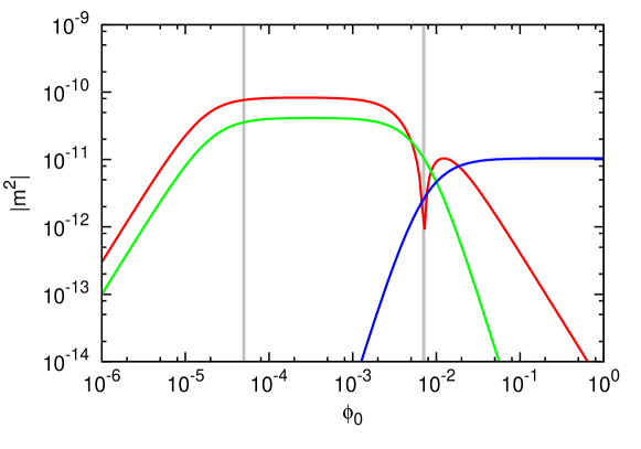
Figure 1: Particle masses $|m^{2}(\phi_{0})|$ as a function of the Higgs vev $\phi_{0}$. Shown are the real Higgs mass (red) and the GB mass (green). In addition the Hubble scale $H^{2}$ is indicated (blue). The two vertical lines correspond to $\phi_{0}=1/\sqrt{\xi}$ and $\phi_{0}=1/\xi$ respectively. Parameters used are $\lambda=0.1$ and $\xi=2\times 10^{4}$.

For the RGEs, the results in the small and mid-field regime are easily generalised to a complex scalar field. The only thing to do is add the contribution of the GB to the CW potential using the expression for the mass, (60). In the small field regime this gives the replacements

$$\beta_{\lambda} =\frac{9}{8\pi^{2}}\lambda^{2}\hskip 5.59998pt\to\frac{9+1}{8\pi^{2}}\lambda^{2},$$ (61)

$$\beta_{\xi} =\frac{36}{16\pi^{2}}\lambda\xi\to\frac{36+3}{16\pi^{2}}\lambda\xi.$$ (62)

To obtain the expression for $\beta_{\xi}$ we again went to order $h^{6}$ in the potential. For the mid-field regime, the CW corrections only enter at order $\delta^{2}$ relative to the leading order term from the classical potential (being conservative with the induced cosmological constant). To lowest order we therefore find the same result as for the real scalar:

$$\beta_{\lambda}=0+\mathcal{O}(\delta^{2}),\quad\beta_{\xi}=\mathcal{O}(\delta^{-1}).$$ (63)

In the large field regime we can work at the lowest order in the expansion, neglecting the back reaction from gravity. Both the Higgs radial mode and the GB are light, with their mass dominated by Hubble corrections and $\hat{m}_{h,\theta}^{2}\approx-2a^{2}H^{2}$. This implies that their propagators have the same form. The equation that determines the beta function, (30), generalises to

$$\beta_{\bar{\lambda}}\partial_{\bar{\lambda}}V_{h}^{\rm cl}=-\partial_{\ln\mu}\frac{1}{2}(V_{hhh}+V_{h\theta\theta})G(0).$$ (64)

Since $V_{hhh}=\mathcal{O}(\delta)$ and $V_{h\theta\theta}=-2\bar{\lambda}\delta^{2}/(3\sqrt{6})=\mathcal{O}(\delta^{2})$, we can neglect the GB contribution. This could have been foreseen from Fig. 1, which shows that the GB mass is parametrically smaller in the large field regime than the Higgs mass (and thus so is the derivative). The beta function in the large field regime is therefore the same for a real and complex scalar.

In summary, the only modification to the beta functions due to the inclusion of a GB is a change in $\beta_{\lambda}$ and $\beta_{\xi}$ in the small field regime. This change is easily generalisable to having $n_{\theta}$ GBs (as needed for a Higgs doublet), and in this case the running of $\lambda$ over the full range is

$$\beta_{\lambda}=\lambda^{2}\times\left\{\frac{9+n_{\theta}}{8\pi^{2}},\;\mathcal{O}(\xi^{-1}),\;-\frac{1}{144\pi^{2}\xi^{2}}\right\}.$$ (65)

6 On the unitarity bound

There is a large and ongoing discussion in the literature regarding the unitarity bound in Higgs inflation, see for example Refs. [8, 24, 25, 26, 30, 34]. The large non-minimal coupling $\xi$ leads to loss of unitarity of $\text{SU}(2)$ gauge boson scattering, and this occurs at an energy which depends on the value of the background Higgs field. In the small and mid-field regime the unitarity bound is below the Planck scale, which suggests new physics, aside from quantum gravity, should enter to restore unitarity at this scale. (Typical energy scales are however always below the scale of unitarity violation.) The minimal assumption is a strong phase of the theory [7, 8]; another option is adding new fields and couplings, see for example Refs. [31, 35] for new interactions that restore unitarity. Whilst we do not have a complete answer to these issues, we would like to make here a brief, and fairly speculative, comment that the new physics necessarily appears only at Planck-scale energies, and, as such, gravity may be enough to UV complete the theory.

Consider scattering two Higgs particles with high momenta while keeping the background Higgs field in the minimum of the Mexican hat potential, i.e., scattering at high energy while remaining in the small field regime. It is far from obvious you can do this. Starting in the small field regime, as you increase kinetic energy you are able to, and in fact with quantum mechanical fluctuations must, probe the large field regime of the potential. This excites background field quanta in the region of the hard scattering interaction point, and so moves the theory into the large field regime at that point.

Following this reasoning, energy is equipartitioned over gradient and potential energy, and it only makes sense to talk about scattering at a given energy when the background field value is also of order this energy — rather than make a distinction between kinetic and potential energy. (In a QFT calculation it seems you can keep the background $\phi$ fixed by hand; however, then this ‘equipartitioning’ should show up if you take higher order corrections into account.) This means you can never probe the small field unitary bound, it is an unphysical bound. As you approach it you must take higher loop corrections into account, and doing that properly it may turn out that no new physics is needed to keep the theory unitary. The real cutoff of the theory can then be pushed to the Planck scale (since that is the cutoff in the large field regime [8]) where gravity corrections are assumed to UV complete the theory.

7 Conclusions

In this paper we have performed a detailed analysis of the quantum corrections and renormalisation in Higgs inflation, computing the beta functions for the couplings $\lambda$ and $\xi$, and the (RG improved) effective potential. We have also given particular attention to the differences between, and compatibility of, the Jordan and Einstein frames.

Working in the Einstein frame, we have computed the beta functions of $\lambda$ and $\xi$ in the small, mid- and large field regimes, finding results that match consistently between the regimes; see Sec. 3. In the small field regime, $\lambda$ runs as it does in the standard model, and we find the beta function for $\xi$ by examining the leading-order irrelevant operator. The mid-field regime is non-renormalisable and, whilst the beta functions depend on the UV completion of the theory, we can still give conservative bounds on them. In the large field regime renormalisability is restored thanks to the approximate shift symmetry and it is the combination $\lambda/\xi^{2}$ that runs.

The theory of Higgs inflation is not renormalisable in the Einstein frame, and so by the assumed quantum-equivalence, the Jordan frame must also be non-renormalisable. In the Einstein frame one can keep gravity as a classical background with minimal error, and treat the action as an EFT, so it is in this frame that calculations are easiest. Even though the theory is non-renormalisable we are still able to make predictions for the beta functions, as the higher order terms are negligible: in small field they are suppressed in the IR; in mid-field they are not computable but are bounded; in large field there is a shift symmetry.

In the literature an alternative way to compute the running uses the s-suppression factor [9, 13, 14]. For this, one should go to the Einstein frame, define $\pi=\partial L/\partial\dot{\phi}$, and apply the usual commutation relations. Note that the Einstein field $\phi$ here does not have a canonical kinetic term. One finds that $[\phi,\dot{\phi}]=is\delta(\vec{x}-\vec{y})$. This leads to the heuristic that all Higgs propagators are suppressed by the field-dependent $s$-factor

$$s(\phi)=\frac{1+\xi\phi^{2}}{1+(1+6\xi)\xi\phi^{2}}.$$ (66)

In the small field regime $s\sim 1$ and the running is as per the SM. For large field, $s\sim 1/6\xi$ acts as to suppress Higgs loops. The CW potential is the calculated in the Jordan frame, using the $s$-factor to account for the non-minimal kinetic terms of the Higgs. While this prescription gives the correct qualitative behaviour — that the contribution of the Higgs field to the effective potential is suppressed in the mid- and large field regime — the exact expression differs from our results. Moreover, it is unclear how to incorporate the GB in this prescription.

Our approach to including GBs in the effective potential and beta functions is to compute their masses using the generalisation of the second derivative of the potential, but in a curved field-space, (20). We have shown explicitly how this works by studying the extension of the model to a complex scalar. The GBs are massive because the Higgs is not in its minimum, and they are suppressed during inflation, as is the Higgs radial mode. In contrast, Refs. [12, 14, 13] claim that only the Higgs field is be suppressed, not the GBs.

At the classical level, it is widely agreed that the Jordan and Einstein frame are equivalent, as going back and forth between them amounts to a redefinition of the fields (the metric and Higgs). However, we also claim that when quantum corrections to the potential are included both frames still give equivalent results for all physical quantities. This is in contrast to claims made in the literature. In some of these works, Refs. [6, 14], it seems that the disagreement follows from neglecting the transformation of the renormalisation point $\mu$ and cutoff $\Lambda$. In Refs. [6, 10, 12, 13, 21, 22, 23] it is the exclusion of gravitational back reaction in the Jordan frame that we do not agree with. Also in Ref. [9] the RGE for $\xi$ is computed with gravity classical in the Jordan frame. We claim that gravitational back reaction, computed in Sec. 2.1, can only be safely ignored in the Einstein frame.

We note that a definitive proof of the quantum equivalence between the Jordan and Einstein frames (or any other frame connected by a conformal rescaling of the metric) should include a proper quantisation, of position and conjugate momentum, in the Jordan frame, from which loop corrections and $n$-point functions should be computed. We are not aware of any work that has carried out this task. So far it seems that the quantisation has always been of one-and-the-same Sasaki-Mukhanov variable. However, we do not see any reason to expect that such a proper quantum computation would reveal a breakdown of the equivalence between the Jordan and Einstein frames. Although our toy model in subsection 4.1 does not take Higgs fluctuations into account, it demonstrates how to correct previous arguments that make claims against quantum frame equivalence.

In regards to unitarity of Higgs inflation, we commented on the possibility that, due to equipartitioning of energy over gradient and potential energy, the new physics required to restore unitarity appears only at Planck-scale energies. As such, quantum gravity may be enough to keep the theory unitary at all energies.

In this paper we have focused on a real Higgs field, with a brief but important extension to the complex case to include GBs. This reduced model retained all the important physics and allowed us to make our points above. Building on this work, we now plan to address the case of the renormalisation of the full standard model Higgs inflation in a follow-up paper.

References

- [1] D. S. Salopek, J. R. Bond, J. M. Bardeen, Phys. Rev. D40 (1989) 1753.
- [2] F. L. Bezrukov, M. Shaposhnikov, Phys. Lett. B659 (2008) 703-706. [arXiv:0710.3755 [hep-th]].
- [3] R. Fakir and W. G. Unruh, Phys. Rev. D 41 (1990) 1783.
- [4] D. I. Kaiser, Phys. Rev. D 52 (1995) 4295 [astro-ph/9408044].
- [5] F. Bezrukov, D. Gorbunov, M. Shaposhnikov, JCAP 0906 (2009) 029. [arXiv:0812.3622 [hep-ph]].
- [6] F. L. Bezrukov, A. Magnin and M. Shaposhnikov, Phys. Lett. B 675 (2009) 88 [arXiv:0812.4950 [hep-ph]].
- [7] F. Bezrukov, M. Shaposhnikov, JHEP 0907 (2009) 089. [arXiv:0904.1537 [hep-ph]].
- [8] F. Bezrukov, A. Magnin, M. Shaposhnikov and S. Sibiryakov, JHEP 1101 (2011) 016 [arXiv:1008.5157 [hep-ph]].
- [9] A. De Simone, M. P. Hertzberg and F. Wilczek, Phys. Lett. B 678 (2009) 1 [arXiv:0812.4946 [hep-ph]].
- [10] A. O. Barvinsky, A. Y. .Kamenshchik and A. A. Starobinsky, JCAP 0811 (2008) 021 [arXiv:0809.2104 [hep-ph]].
- [11] A. O. Barvinsky, A. Y. .Kamenshchik, C. Kiefer, A. A. Starobinsky and C. Steinwachs, JCAP 0912 (2009) 003 [arXiv:0904.1698 [hep-ph]].
- [12] A. O. Barvinsky, A. Y. .Kamenshchik, C. Kiefer, A. A. Starobinsky and C. F. Steinwachs, Eur. Phys. J. C 72 (2012) 2219 [arXiv:0910.1041 [hep-ph]].
- [13] R. N. Lerner and J. McDonald, Phys. Rev. D 80 (2009) 123507 [arXiv:0909.0520 [hep-ph]].
- [14] K. Allison, arXiv:1306.6931 [hep-ph].
- [15] D. I. Kaiser, [astro-ph/9507048].
- [16] E. E. Flanagan, Class. Quant. Grav. 21 (2004) 3817 [gr-qc/0403063].
- [17] J. Weenink and T. Prokopec, Phys. Rev. D 82 (2010) 123510 [arXiv:1007.2133 [hep-th]].
- [18] T. Prokopec and J. Weenink, arXiv:1304.6737 [gr-qc].
- [19] J. White, M. Minamitsuji and M. Sasaki, JCAP 1207, 039 (2012) [arXiv:1205.0656 [astro-ph.CO]].
- [20] J. White, M. Minamitsuji and M. Sasaki, JCAP 1309, 015 (2013) [arXiv:1306.6186 [astro-ph.CO]].
- [21] T. Markkanen and A. Tranberg, JCAP 1211 (2012) 027 [arXiv:1207.2179 [gr-qc]].
- [22] I. L. Buchbinder, S. D. Odintsov and I. L. Shapiro, Bristol, UK: IOP (1992) 413 p
- [23] K. Kirsten, G. Cognola and L. Vanzo, Phys. Rev. D 48 (1993) 2813 [hep-th/9304092].
- [24] J. L. F. Barbon, J. R. Espinosa, Phys. Rev. D79 (2009) 081302 [arXiv:0903.0355 [hep-ph]]
- [25] C. P. Burgess, H. M. Lee and M. Trott, JHEP 0909 (2009) 103 [arXiv:0902.4465 [hep-ph]].
- [26] C. P. Burgess, H. M. Lee and M. Trott, JHEP 1007 (2010) 007 [arXiv:1002.2730 [hep-ph]].
- [27] S. Ferrara, R. Kallosh, A. Linde, A. Marrani and A. Van Proeyen, Phys. Rev. D 83 (2011) 025008 [arXiv:1008.2942 [hep-th]].
- [28] S. Mooij and M. Postma, JCAP 1109 (2011) 006 [arXiv:1104.4897 [hep-ph]].
- [29] D. P. George, S. Mooij and M. Postma, JCAP 1211 (2012) 043 [arXiv:1207.6963 [hep-th]].
- [30] M. P. Hertzberg, JHEP 1011 (2010) 023 [arXiv:1002.2995 [hep-ph]].
- [31] G. F. Giudice and H. M. Lee, Phys. Lett. B 694 (2011) 294 [arXiv:1010.1417 [hep-ph]].
- [32] D. I. Kaiser, Phys. Rev. D 81 (2010) 084044 [arXiv:1003.1159 [gr-qc]].
- [33] P. A. R. Ade et al. [Planck Collaboration], arXiv:1303.5076 [astro-ph.CO].
- [34] R. N. Lerner and J. McDonald, JCAP 1004 (2010) 015 [arXiv:0912.5463 [hep-ph]].
- [35] R. N. Lerner and J. McDonald, Phys. Rev. D 82 (2010) 103525 [arXiv:1005.2978 [hep-ph]].
- [36] S. R. Coleman, E. J. Weinberg, Phys. Rev. D7 (1973) 1888-1910.
- [37] G. Aad et al. [ATLAS Collaboration], Phys. Lett. B 716 (2012) 1 [arXiv:1207.7214 [hep-ex]].
- [38] S. Chatrchyan et al. [CMS Collaboration], Phys. Lett. B 716 (2012) 30 [arXiv:1207.7235 [hep-ex]].
- [39] F. Bezrukov, M. Y. .Kalmykov, B. A. Kniehl and M. Shaposhnikov, JHEP 1210, 140 (2012) [arXiv:1205.2893 [hep-ph]].
- [40] G. Degrassi, S. Di Vita, J. Elias-Miro, J. R. Espinosa, G. F. Giudice, G. Isidori and A. Strumia, JHEP 1208, 098 (2012) [arXiv:1205.6497 [hep-ph]].
- [41] D. Buttazzo, G. Degrassi, P. P. Giardino, G. F. Giudice, F. Sala, A. Salvio and A. Strumia, arXiv:1307.3536 [hep-ph].
- [42] O. Lebedev, Eur. Phys. J. C 72 (2012) 2058 [arXiv:1203.0156 [hep-ph]].
- [43] J. Elias-Miro, J. R. Espinosa, G. F. Giudice, H. M. Lee and A. Strumia, JHEP 1206 (2012) 031 [arXiv:1203.0237 [hep-ph]].
- [44] V. F. Mukhanov and G. V. Chibisov, JETP Lett. 33 (1981) 532 [Pisma Zh. Eksp. Teor. Fiz. 33 (1981) 549].
- [45] V. F. Mukhanov, H. A. Feldman and R. H. Brandenberger, Phys. Rept. 215 (1992) 203.
- [46] H. Kodama and M. Sasaki, Prog. Theor. Phys. Suppl. 78 (1984) 1.
- [47] M. S. Sloth, Nucl. Phys. B 775 (2007) 78 [hep-th/0612138].
- [48] M. Sher, Phys. Rept. 179 (1989) 273.