On detecting interactions in the dark sector with $H(z)$ data

Abstract

An interesting approach to the cosmological coincidence problem is to allow dark matter and dark energy interact with each other also nongravitationally. We consider two general Ansätze for such an interaction and appraise their ability to address the coincidence problem. We determine the average accuracy required on the cosmic expansion rate data to distinguish interacting cosmological models from the conventional $\Lambda$CDM scenario. We find that among the planned surveys the Wide Field Infrared Survey Telescope has the best chance to detect an interaction, though at a low significance level. To unambiguously determine the existence of an interaction one must, therefore, combine the said expansion data with other probes.

I Introduction

After many years of research very little is known for certain about the two components of the dark sector: cold dark matter (DM) and dark energy (DE). The latter, possibly in the form of a cosmological constant, appears to be the agent driving the current phase of cosmic accelerated expansion. Thus, some basic questions immediately arise. For instance, is the cosmological constant a manifestation of the quantum vacuum? If so, the huge gap between the DE density expected from quantum field theory and the observed one is in urgent need of explanation Weinberg1989 . Likewise, why are the densities of DM and DE of the same order precisely today? Why are we living in such a special epoch i.e., “why now?” This constitutes the so-called “coincidence problem”. Also, do DM and DE interact gravitationally only or are they coupled? There is little doubt that these fundamental questions must be interrelated whereby shedding light on one of them may help to explain the others. Following this line of thought we focus on the why now problem, hoping that if it is better understood, it will mean a major step in unveiling the nature of the components of the dark sector. Notice that because of our current lack of knowledge about the nature of these two components it would be unwise to discard a priori an interaction among them. What is more, they should be coupled unless some so far unknown-symmetry forbids it. Besides, data obtained from observations of the dynamics of galaxy clusters elcio and the integrated Sachs-Wolfe effect german hint that indeed they interact with one another, DE slowly decaying in DM.

To the best of our knowledge, the first proposal on theoretical grounds that what we now call dark energy may decay into matter and radiation was made as early as 1933 by Bronstein Bronstein1933 . Later on, Wetterich christoff , Micheletti, Abdalla, and Wang sandro , Polyakov polyakov , and Abdalla, Graef, and Wang elcio-bin , among others, reinforced the theoretical framework. As we write, the number of proposals (both from the theoretical as well as from the phenomenological side) has been greatly augmented -see e.g. Overduim1998 ; Luca2000 ; Amendola-book , and references therein.

Here we shall assume that the Universe is homogeneous and isotropic at large scales, with flat spatial sections, dominated by nonbaryonic cold matter, by dark energy, and (to a lesser extent) by baryons (subscripts $m$, $x$, and $b$, respectively). We neglect radiation, as it results as dynamically unimportant at the epochs we are interested in.

The overall energy conservation equation reads

$$\dot{\rho}+3H(\rho+p)=0,$$ (1)

where $\rho=\rho_{b}+\rho_{m}+\rho_{x}$, $p$ denotes the total pressure of the cosmic fluid, and $H$ is the Hubble factor. In the customary description of the expansion DM and DE evolve independently, as no interaction other than gravity is considered. However, there is no apparent reason why they should not interact. So, in general, they must couple through some small term $Q$:

$$\dot{\rho}_{m}+3H\rho_{m}=Q\,,$$ (2)

$$\dot{\rho}_{x}+3H(1+w)\rho_{x}=-Q\,.$$ (3)

Here $w=p_{x}/\rho_{x}<-1/3$ is the equation of state parameter of DE, which for the sake of easiness we will assume to be constant. Notice that the last two equations, together with the independent conservation of $\rho_{b}$, guarantee the fulfilment of (1).

The next section introduces, on a phenomenological basis, appropriate expressions for $Q$ restricted by the conditions of simplicity, smallness, and positivity. The latter comes from the result that a negative $Q$ would violate the second law of thermodynamics secondlaw ; i.e., the energy transfer must go from DE to DM, not the other way around, in conformity with the findings of Refs. elcio ; german . Likewise, $Q$ must be small (i.e., it should be bound by $Q/3H\rho_{m}<1$); otherwise, the DM could still dominate the expansion today.

A key quantity in interacting scenarios is the ratio between DM and DE, $r=\rho_{m}/\rho_{x}$. In general, we expect it to monotonically decrease with expansion. Equations (2) and (3) imply

$$\frac{\dot{r}}{r}=3Hw\,+\,(1+r)\,\frac{Q}{\rho_{x}}\,.$$ (4)

Thus, the coincidence problem will be alleviated if $r$ decreases with expansion slower than in the conventional $\Lambda$CDM model, and much more so if for an extended expanse of time around the present epoch the right-hand side of the last expression stays close to zero. Obviously, for any of them to occur, $Q$ must be positive definite. In general, $\dot{r}$ should be negative at all times. This leads to a further upper bound on $Q$:

$$Q\leq-3Hw\,\frac{\rho_{x}}{1+r}\,,$$ (5)

that may well be satisfied. Indeed, at early times one expects $r$ and $H$ to be much larger than their respective current values; and at times later than the present one, one expects both of them to be smaller. In general, if it were not so (i.e., if $\dot{r}$ were positive at late times), then the deceleration parameter, $q=-1-(\dot{H}/H^{2})$, some time in the future would evolve from negative to positive values, conflicting with the second law of thermodynamics grg-nd . Thus, the bound above is not at all unreasonable.

The aim of this paper is twofold: first, to explore to what extent some specific interactions terms (i.e., Q) alleviate the coincidence problem and, second, to investigate how accurate measurements of $H(z)$ must be to tell us, for the chosen Asätze, whether there really is an interaction in the dark sector.

We believe this research is well justified in view of the progress made in the recent years on the observational side. Indeed, it is not an exaggeration to say that we are living in an exciting time for cosmology. Currently, there are a number of ongoing surveys and many more are planned -see Sec. 14 of Ref. li-li . The assured result is that the frontier of our knowledge on cosmology will be pushed rather far away. In the next two decades, measurements of $H(z)$ will be improved from the current accuracy of roughly $12\%$ to better than $1\%$. This will allow one to test cosmological models with unprecedented confidence.

The outline of the paper is as follows: Section II presents two classes of interactions (I and II) and recalls the solutions to the conservation equations for the interaction Ansätze adopted that have analytical solution. Section III investigates whether these models really address the coincidence problem. Section IV makes forecasts about detecting an interaction based on measurements of the Hubble parameter. Section V summarizes our findings and makes some final comments. As is usual, a subscript zero denotes the current value of the corresponding quantity.

II Interacting models

¿From Eqs. (2) and (3), $Q$ must be a function of the energy densities multiplied by a quantity with units of inverse of time. For the latter we may take the Hubble expansion rate; thus, $Q=Q(H\rho_{m},H\rho_{x})$. By power-law expanding last expression and retaining just the first term, we arrive to the first class of interacting models:

$$\mbox{I}:\;\;Q_{1}=3H(\epsilon_{m}\rho_{m}+\epsilon_{x}\rho_{x})\,,$$ (6)

where the parameters $\epsilon_{m}$ and $\epsilon_{x}$ are small positive-semidefinite constants. This class, with $\epsilon_{m}=\epsilon_{x}>0$, leads a constant ratio, $r$, at late times, thus solving the coincidence problem Chimento2003a ; Chimento2003b .

As a further class we consider

$$\mbox{II}:\;\;Q_{2}=3(\Gamma_{m}\rho_{m}+\Gamma_{x}\rho_{x})\,,$$ (7)

where $\Gamma_{m}$ and $\Gamma_{x}$ are non-negative, small, constant time rates (by “small” we mean smaller than $H_{0}$). Cosmological models featuring this type of interaction in the dark sector are motivated by similar models in reheating, curvaton decay, and decay of DM into radiation Caldera-Cabral2009 .

Throughout this paper we will adopt the following specific Ansätze for the DM-DE interaction, Eqs. (6) and (7):

$$Q_{1a}=3\epsilon H\rho_{m}\,,$$ (8)

$$Q_{1b}=3\epsilon H\rho_{x}\,,$$ (9)

$$Q_{1c}=3\epsilon H(\rho_{m}+\rho_{x})\,,$$ (10)

$$Q_{2a}=3\Gamma\rho_{m}\,,$$ (11)

$$Q_{2b}=3\Gamma\rho_{x}\,,$$ (12)

$$Q_{2c}=3\Gamma(\rho_{m}+\rho_{x})\,.$$ (13)

Models of type I explicitly depend on $H(z)$, while type II models do not. The conservation equations for models of type I have analytical solutions for all three cases considered (see, for example, delCampo2011 ). We next recall them.

II.1 Ansatz $Q_{1a}$

$$\rho_{m}=\rho_{m0}\;x^{3(1-\epsilon)},$$ (14)

$$\rho_{x}=\rho_{x0}\;x^{3(1+w)}+\left(\frac{\epsilon}{\epsilon+w}\right)\rho_{m0}[x^{3(1+w)}-x^{3(1-\epsilon)}],$$ (15)

where $x=1+z=\frac{a_{0}}{a}$ with $a$ the scale factor of the Friedmann-Robertson-Walker metric.

II.2 Ansatz $Q_{1b}$

$$\rho_{m}=\rho_{m0}\;x^{3}+\left(\frac{\epsilon}{\epsilon+w}\right)\rho_{x0}[1-x^{3(w+\epsilon)}]x^{3}\,,$$ (16)

$$\rho_{x}=\rho_{x0}\;x^{3(1+w+\epsilon)}\,.$$ (17)

II.3 Ansatz $Q_{1c}$

$$\rho_{m}=C_{1}x^{\gamma_{1}}+C_{2}x^{\gamma_{2}}\,,$$ (18)

$$\rho_{x}=\frac{1}{2\epsilon}\left[-C_{1}(A+B)+C_{2}(B-A)x^{-3B}\right]x^{\gamma_{1}}\,,$$ (19)

where $C_{1,2}$, $\gamma_{1,2}$, $A$ and $B$ are defined below:

$$\gamma_{1}=\frac{3}{2}(2+w+B)\,,\;\quad\gamma_{2}=\frac{3}{2}(2+w-B)\,,$$ (20)

$$C_{1}=\frac{1}{2B}[(B-A)\rho_{m0}-2\epsilon\rho_{x0}],\;\quad C_{2}=\frac{1}{2B}[(B+A)\rho_{m0}+2\epsilon\rho_{x0}],$$ (21)

$$A=w+2\epsilon,\;\quad B=\sqrt{w(w+4\epsilon)}\,.$$ (22)

Models of type II$a$ and II$b$ have an analytical solution for just one of the conservation equations (for $\rho_{m}$ in case II$a$ and for $\rho_{x}$ in case II$b$, see Caldera-Cabral2009 ), while model II$c$ [Eq. (13)] has no analytical solution. In any case, they are to be solved numerically.

Table 1 recalls some of the observational constraints of type I models – see Refs. He2011 ; Basilakos2009 ; Costa2010 . To the best of our knowledge no observational constraints for model II are known at this stage.

Reference	$Q_{1a}$	$Q_{1b}$	$Q_{1c}$
He2011 $(w<-1)$	$\epsilon=0.0006^{+0.0006}_{-0.0005}$	$\epsilon=0.024^{+0.034}_{-0.027}$	$\epsilon=0.0006^{+0.0005}_{-0.0006}$
He2011 $(w>-1)$	None	$\epsilon=-0.003^{+0.017}_{-0.024}$	None
Basilakos2009 $(w=-1)$	$\epsilon=0.002\pm 0.001$	None	None
Costa2010 $(w=-1)$	$\epsilon=0.01\pm 0.01$	None	None

Table 1: Observational constraints on $\epsilon$ for type I models.

III Alleviating the coincidence problem

As said above, an interaction in the dark sector, aside from being an open theoretical option, provides an interesting possibility to address the coincidence problem. This section focus on how the interacting Asätze given by Eqs. (8)-(13) fare with that issue by determining (analytically for class I models and numerically for class II models) the evolution of the ratio $r=\frac{\rho_{m}}{\rho_{x}}$, whose present day value $r_{0}$ is of the order of the unity. The coincidence problem will be alleviated if $r\simeq r_{0}$ for a substantially longer period about the present time than in the $\Lambda$CDM model. This has been investigated in some extent in references delCampo2008 -He2009 .

Figures 2 and 2 plot $r\,$ vs $\,1+z$ (with $w=-1.0$) for models of type I and II, respectively. They result from integrating the conservation equations (2) and (3), in each case using the corresponding expression for $Q$. The values of $\epsilon$ were selected to span current constraints (see Table 1) and those corresponding to $\Gamma/H_{0}$ were set to the same set of values.

Throughout this paper we take $H_{0}=67.4$, $\Omega_{b0}=0.049$, $\Omega_{m0}=0.265$, and $\Omega_{x0}=1-\Omega_{m0}-\Omega_{b0}$, the central values reported by the Planck Collaboration PlanckCosmo2013 , and, accordingly, we use $r_{0}=0.386$. As usual, the $\Omega$ quantities denote fractional densities.

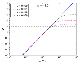
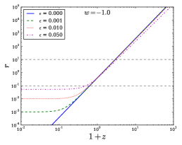
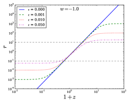
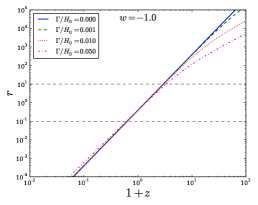
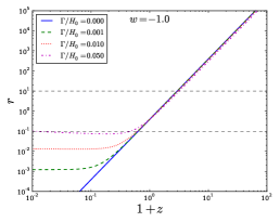
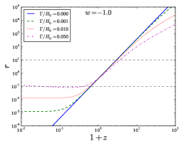
Figure 1: Plots of $r$ as a function of $1+z$ for Asätze $Q_{1a}$ (left panel), $Q_{1b}$ (middle panel) and $Q_{1c}$ (right panel). The dashed horizontal lines correspond to $r=0.1$ and $r=10$. As can be seen from Eq. (19), model $Q_{1c}$ has an apparent divergence for $\epsilon=0$ (analytic computation of the limit $\epsilon\rightarrow 0$ shows that it really exists), so we put a very small value for $\epsilon$ that represents the $\Lambda$CDM for comparison purposes. In plotting the graphs we used $H_{0}=67.4$, $\Omega_{b}=0.049$, $\Omega_{m}=0.265$ and $\Omega_{x}=1-\Omega_{m}-\Omega_{b}$.

Figure 2: The same as Fig. 2 but for the Ansätze $Q_{2a}$ (left panel), $Q_{2b}$ (middle panel), and $Q_{2c}$ (right panel).

¿From Fig. 2 [that corresponds to models of type I, directly depending on $H(z)$], it is seen that $r$ deviates from the $\Lambda$CDM model at different redshift intervals depending on the form of the interaction. When $Q$ depends on $\rho_{m}$, $r$ deviates in the matter-dominated region (left panel). When $Q\propto\rho_{x}$ the deviation occurs mostly in the future ($z<0$), where dark energy prevails (middle panel). Finally, when $Q\propto(\rho_{m}+\rho_{x})$, right panel, the deviations occur both in the past and in the future. Although the curves for $r$ in the interacting model look almost the same as for the $\Lambda$CDM model in the vicinity of the present age (horizontal dashed lines in Fig. 2), they limit the range which $r$ varies in the past (left panel), future (middle panel), or both past and future (right panel). While this does not help to clarify why $r$ is of the order of unity today, it narrows the range $r$ spans. For instance, model $Q_{1c}$ (right panel of Fig. 2) limits $r$ in the range $10^{-3}$ - $10^{3}$ (for $\epsilon=0.001$), thus alleviating the coincidence problem. Similarly, models $Q_{1a}$ (left panel) and $Q_{1b}$ (middle panel) narrow the allowed range of $r$ in the past and future, respectively. In this sense, all three Asätze alleviate the coincidence problem for positive values of $\epsilon$ (negative values only worsen the problem). More specifically, from the middle panel of said figure we learn that at the very far future, $z=-0.99$, $r$ takes values not lower than $10^{-3}$ for the interacting models displayed in that panel, but for the $\Lambda$CDM it goes down to $10^{-6}$. Like comments apply to the right-hand panel.

As is well known, the contribution of dark energy (with constant $w$) at high redshifts is substantially constrained bean ; xia-viel . Combining a variety of observational data, Xia and Viel xia-viel found that the fractional density of dark energy at the time of last scattering surface should not exceed $1.4\times 10^{-3}$ (at $95\%$ confidence level). This implies that in the case of Ansätze $Q_{1a}$ and $Q_{1c}$ (left and right panels of Fig. 2, respectively) $\epsilon$ should be of the order of $10^{-3}$ or less.

Curiously enough, Ansätze $Q_{1b}$ and $Q_{2b}$ lead to very similar evolutions of $r$, particularly for $z<0$. Figure 2 [corresponding to models of type II, which do not directly depend on $H(z)$] shows that the Ansatz $Q_{2a}$ barely alleviates the coincidence problem (left panel), for it does not limit $r$ in either the past or future. The other two Ansätze (middle and right panels) do alleviate it, limiting $r$ in the future (in a similar way of the Ansätze of Fig. 2). We also notice the same features mentioned above for models of type I (Fig. 2), explaining the deviations of $r$ from $\Lambda$CDM according to the dependencies of $Q$ ($\rho_{m}$, $\rho_{x}$ or $\rho_{m}+\rho_{x}$). By contrast to Caldera-Cabral2009 , we see that interactions of type II (Ansatz $Q_{2c}$ with $w=-1$, right panel of Fig. 2) are well behaved at all times and also address the coincidence problem, as long as $\Gamma/H_{0}\lesssim 0.01$, when $r$ is also well behaved up to at least $1+z=10^{-15}$. The same holds true for the claim in Caldera-Cabral2009 that in the case of the Ansatz $Q_{2b}$ the Universe would be dominated by DM in the future: If $\Gamma/H_{0}\lesssim 0.01$, we find that DE dominates until at least $1+z=10^{-15}$.

¿From Figs. 2 and 2 we conclude that for $\epsilon\simeq\Gamma/H_{0}$ the evolution of $r$ does not greatly differ, particularly between the cases $Q_{1b}$ and $Q_{2b}$. This may indicate that the constraints on $\Gamma/H_{0}$ will be of the same order of magnitude as those of $\epsilon$ for corresponding models.

Altogether, we can say that the Ansätze that most alleviate the coincidence problem, and do not conflict with present constraints on the abundance of dark energy at early times, are $Q_{1b}$, $Q_{2b}$, and $Q_{2c}$.

As an example of dependency of the densities ratio $r$ with the equation of state parameter $w$, Fig. 3 shows plots for three values of $w$ for the Ansatz $Q_{2c}$. It is seen that $w<-1$ (phantom values) tends to worsen the coincidence problem, while for $w>-1$ (quintessence values) it gets alleviated. It should be recalled that, in addition, phantom models face severe problems regarding quantum stability hoffman ; cline and violate the second law of thermodynamics grg-nd . Likewise, we wish to emphasize that in order not to run into negative $\rho_{x}$ values, $\Gamma/H_{0}$ must be lower than $\sim\,10^{-4}$ and $10^{-2}$ for $w=-0.9$ and $w=-1$, respectively.

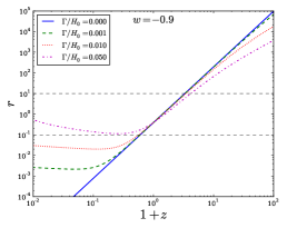
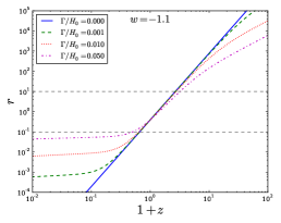
Figure 3: Dependence on $w$ for Ansatz $Q_{2c}$ when $w=-0.9$ (left panel), $w=-1.0$ (middle panel) and $w=-1.1$ (right panel). In plotting the graphs we used $H_{0}=67.4$, $\Omega_{b}=0.049$, $\Omega_{m}=0.265$, and $\Omega_{x}=1-\Omega_{m}-\Omega_{b}$.

IV Forecasts for detecting an interaction through $H(z)$ data

In this section, we investigate the possibility of detecting an interaction, i.e., whether DE and DM interact also nongravitationally with each other, by using $H(z)$ data only. In Ferreira2013 it was investigated for the specific Ansatz $Q_{1a}$ with $w=-1$. Here we extend that analysis for the models described in Sect. II, for constant $w$.

The error associated in measuring $H(z,\epsilon)$ propagates according to

$$\delta H^{2}=\left(\frac{\partial H}{\partial\epsilon}\right)^{2}\delta\epsilon^{2}\,,$$ (23)

and to an analogous expression for $H(z,\Gamma)$. Thus, with the help of the last equation, one can calculate how the error in $H(z)$ data propagates to $\epsilon$ (and correspondingly to $\Gamma/H_{0}$) as a function of redshift. To allow a direct and unambiguous forecast we compute the average of the relative H(z) error, $\delta H/H$, over redshift [Eq. 5 of Ferreira2013 ]:

$$\left<\frac{\delta H}{H}\right>=\left[\frac{1}{z_{f}-z_{i}}\int_{z_{i}}^{z_{f}}\frac{1}{H}\left|\frac{\partial H}{\partial\epsilon}\right|dz\right]\delta\epsilon\;,$$ (24)

where [$z_{i}$, $z_{f}$] is the redshift interval in which the data happen to fall. A corresponding expression holds for the case of models belonging to class II. Here we take $z_{i}=0.07$ and $z_{f}=2.3$, that fix the interval of the most recent data - see Table 1 in Ref. Farooq2013 . By calculating the average over redshift, we allow a direct estimate for the required accuracy in $H(z)$ observations to detect a given interaction. The quantities $\partial H/\partial\epsilon$ were computed analytically; the quantities $\partial H/\partial\Gamma$, numerically. Equation (24) (and their corresponding one for models of class II) was integrated numerically in all the cases. Note that the outcome of (24) does not depend on the number of data points in the interval.

The results for models of type I are plotted in Figs. 6, 6 and 6 for Ansätze $Q_{1a}$, $Q_{1b}$ and $Q_{1c}$, respectively, for $\epsilon=0.005,0.01,0.02$ and five values of $w$. Likewise, the outcomes for models of type II are plotted in Figs. 9, 9, and 9 for $Q_{2a}$, $Q_{2b}$, and $Q_{2c}$, respectively, for $\Gamma/H_{0}$ and $w$ with the same values as for models of type I. Note that the limiting case where it is possible to tell an interaction with $1\sigma$ confidence level corresponds to $\delta\epsilon/\epsilon=100\%$ ($\delta\Gamma/\Gamma=100\%$).

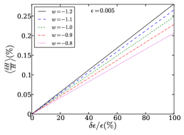
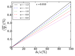
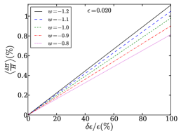
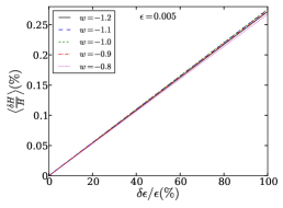
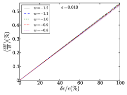
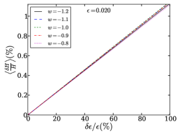
Figure 4: Estimates of $\left<\frac{\delta H}{H}\right>$ for Ansatz $Q_{1a}$, Eq. (8) for three different values of the parameter $\epsilon$.

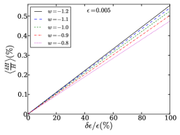
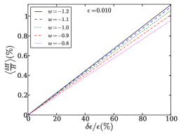
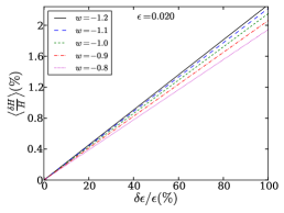
Figure 5: The same as Fig. 6, but for model $Q_{1b}$, Eq. (9).

Figure 6: The same as Fig. 6, but for model $Q_{1c}$, Eq. (10).

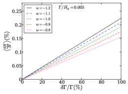
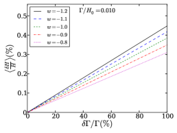
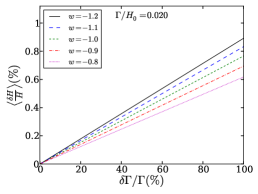
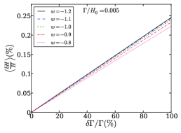
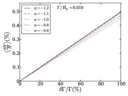
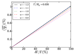
Figure 7: Estimates of $\left<\frac{\delta H}{H}\right>$ for Ansatz $Q_{2a}$, Eq. (11) for three different values of the parameter $\Gamma/H_{0}$.

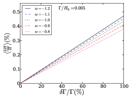
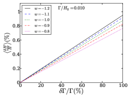
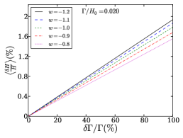
Figure 8: The same as Fig. 9, but for ansatz $Q_{2b}$, Eq. (12).

Figure 9: The same as Fig. 9, but for Ansatz $Q_{2c}$, Eq. (13).

A feature common to Figs. 6-9 is that the more negative $w$ is, the easier it is to detect the interaction (the higher the slope of the graph). An exception is, however, $Q_{1b}$ (Fig. 6), where the case $w=-1.1$ is slightly easier to detect than $w=-1.2$, even though the $w$ dependence is considerably weaker than in the other cases. It is also apparent that for the same value of the interaction parameter ($\epsilon$ or $\Gamma/H_{0}$) it is always easier to distinguish the interaction in models with $Q\propto(\rho_{m}+\rho_{x})$ ($Q_{1c}$ and $Q_{2c}$), which gives $\delta H/H\sim 2$ times larger than for models where $Q\propto\rho_{m}$ or $Q\propto\rho_{x}$.

He, Wang, and Abdalla He2011 determined, for model $Q_{1b}$ (with $w<-1$), that $\epsilon=0.024^{+0.034}_{-0.027}$ (see Table 1). According to Fig. 6 (right panel), it would required an accuracy of about $1.2\%$ in $H(z)$ to measure $\epsilon$ with similar accuracy. Other constraints obtained by the same authors (see Table 1) are considerably more stringent than that for Ansatz $Q_{1b}$ ($w<-1$). Another example: In order to measure $\epsilon$ for model $Q_{1a}$ with the same accuracy as in Costa2010 ($\epsilon=0.01\pm 0.01$, equivalent to $\delta\epsilon/\epsilon=1$; see Table 1), from Fig. 6 (middle panel), an accuracy of $0.5\%$ (for $w=-1$) would be required in measuring $H(z)$.

The results for model II (Figs. 9- 9) are very similar to those of model I (Figs. 6-6), though a slightly better accuracy is needed. For instance, an interaction $\Gamma/H_{0}=0.024$ for Ansatz $Q_{2b}$ could be detected if $\left<\delta H/H\right>\simeq 1\%$ (right panel of Fig. 9), instead of $1.2\%$ in the analogous case of Ansatz $Q_{1b}$ described above.

We next consider how the redshift interval of a data set affects the accuracy required to detect an interaction. Figure 10 plots $\left<\frac{\delta H}{H}\right>$ in terms of $\epsilon$ for the case of Ansatz $Q_{1b}$ for different values of the redshift range of the data. It is seen that the interaction (if it exists) is easier to detect by observing H(z) at higher redshifts. Recently $H$ was measured at $z=2.3$ Busca2013 , extending the previous upper value determined at $z=1.75$ Simon2005 . For instance, an interaction such that $\epsilon=0.02$ could be detected with an $H(z)$ accuracy of $0.8\%$ for $z_{f}=1.5$, whereas if $z_{f}$ were increased to $3.0$, an accuracy of $\sim 1.3\%$ would suffice to detect the interaction. This underlines the importance of measuring $H$ at high redshifts.

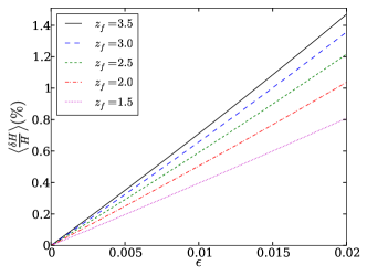
Figure 10: Dependence of $\left<\frac{\delta H}{H}\right>$ with the redshift range of the data set for $\delta\epsilon=\epsilon$, and Ansatz $Q_{1b}$. In plotting the graphs we used $w=-1$, $z_{i}=0.07$ and $\delta\epsilon/\epsilon=100\%$.

IV.1 Future measurements of H(z)

The most recent $H(z)$ data Farooq2013 have an average accuracy of only $\sim 12\%$. This shows how far we are from distinguishing an interaction in the dark sector from the noninteracting case using just $H(z)$ data. Next we briefly review what should be expected from planned surveys.

First, a high accuracy is expected for $H_{0}$. The James Webb Space Telescope, to be launched in 2018, will measure light curves of Cepheid stars further than $50$ Mpc away, thus increasing the number of supernovae calibrators, and may achieve a $1\%$ measurement of $H_{0}$ Gardner2010 .

Crawford et al. estimated the observing time required for the Southern African Large Telescope to measure $H(z)$ for different accuracies Crawford2010 . By using the differential ages method for luminous red galaxies with an extended star formation history, they found that each redshift bin measurement of $H(z)$ would require about $180$ h to reaches $\delta H/H=3\%$. That means an accuracy of $3\%$ may be reached at present, but it would imply a considerable amount of observation time. More promising measures of $H(z)$, using baryon acoustic oscillations, are to come with the Wide Field Infrared Survey Telescope (WFIRST) WFISRT2013 , to be launched in 2020. It will allow one to determine $H(z)$ with an aggregate precision of $0.72\%$ in the redshift interval $1<z<2$ and $1.8\%$ at $2<z<3$. This combination of high accuracy and redshift range will offer a great opportunity not just to probe a likely interaction in the dark sector, but also to test a wide variety of cosmological models.

V Concluding remarks

In this paper we considered two previously studied classes of interacting DM-DE, Eqs. (6) and (7), and used their one-parameter special cases, Eqs. (8)-(13), to study (i) their ability to address the coincidence problem (Sec. III), and (ii) the possibility of detecting an interaction based solely on $H(z)$ observations (Sec. IV). We first studied the effect of the mentioned dark sector interaction forms in the evolution of the ratio $\rho_{m}/\rho_{x}$ and confirmed that a transfer of energy from DM to DE (negative $\epsilon$ or $\Gamma$) only makes the coincidence problem more severe. The coincidence problem gets more alleviated with increasing $\epsilon$ (or $\Gamma$). The Ansätze that fare better with that issue when account is taken also on the bounds on early dark energy xia-viel are $Q_{1b}$ for models of class I and $Q_{2b}$ and $Q_{2c}$ for class II. Likewise, phantom models worsen the problem. A curious fact is that models of type I and II exhibit a like behavior for similar values $\epsilon$ and $\Gamma/H_{0}$, despite the fact that class I depends directly on $H(z)$ while class II does not. We also investigated the influence of the (constant) equation of state parameter $w$ and showed that the coincidence problem gets more alleviated when $w>-1$, though not significantly. On the other hand, phantom cases require smaller values of $\Gamma/H_{0}$ to avoid negative densities in the futures (for Ansätze $Q_{2b}$ and $Q_{2c}$).

We do not claim that models that more alleviate the coincidence problem are closer to the “true” model, but they certainly are more appealing and therefore deserve special attention, from both the theoretical and observational viewpoints. Nevertheless, we are far from a complete picture.

We calculated how the errors in $H(z)$ propagate to the interaction parameters and made several estimates of the possibilities of measuring an interaction, depending on the Ansatz employed (Sec. IV). Models with $Q\propto(\rho_{m}+\rho_{x})$ are detectable with less accuracy (about $2$ times worse) than for the same value of the interaction parameter of models with $Q\propto\rho_{m}$ or $Q\propto\rho_{x}$. Likewise, the equation of state parameter of DE, $w$, may have a considerable influence on the value of $\left<\frac{\delta H}{H}\right>$. In particular, for $w<-1$ the interaction is easier to detect (but, as said above, it worsens the coincidence problem and suffers from others severe drawbacks). We found that if the WFIRST experiment reach an average accuracy of $0.7\%$ up to $z=3.0$, it will be able to see an interaction with $1\sigma$ confidence level of $\epsilon\gtrsim 0.01$ (for $w=-1$) (modulo the interaction exists). According to the constraints of for Ansatz $Q_{1a}$ (Table 1, Ref. Costa2010 ), this value is still allowed by observation. Other model forecasts are discussed in Sec. IV.

We may conclude by saying that the $H(z)$ data should be complemented with data from other sources (such as supernovae type Ia, baryon acoustic oscillations, dynamical evolution of galaxy clusters, integrated Sachs-Wolfe effect, growth factor, etc) to determine with certainty whether DM and DE energy interact with each other also nongravitationally.

Claims were made that in models of class I, with $w>-1$, density perturbations blow up on super-Hubble scales valiviita , no matter how small the coupling parameter, $\epsilon$, might be. The smaller $\epsilon$, the earlier the instability would set in. This defies intuition because, in any case, in the $\epsilon\rightarrow 0$ limit the perturbations should not diverge at all. Recently, a detailed analysis of the energy-momentum transfer between both dark components disproved the claims Sun2013 .

Admittedly, a clear limitation of this work is its restriction to the $w$ constant. It would be interesting to adopt a parametrization for this quantity, such as the one proposed by Chevallier and Polarski chevallier and Linder linder . However, it would introduce a further parameter which would much involve the calculations. In any case, this may well be the subject of a future research.

- (1) S. Weinberg, Rev. Mod. Phys. 61, 1 (1989).
- (2) E. Abdalla, E. R. W. Abramo, L. Sodre, and B. Wang, Phys. Lett. B 673, 107 (2009).
- (3) G. Olivares, F. Atrio-Barandela, and D. Pavón, Phys. Rev. D 77, 103520 (2008).
- (4) M. Bronstein, Phys. Z. Sowjetunion 3, 73 (1933).
- (5) C. Wetterich, Nucl. Phys. B 302, 668 (1988).
- (6) S. Micheletti, E. Abdalla and B. Wang, Phys. Rev. D 79, 123506 (2009).
- (7) A. M. Polyakov, Nucl. Phys. B 834, 316 (2010).
- (8) E. Abdalla, L. Graef, and B. Wang, arXiv:1202.0499 [gr-qc].
- (9) J. Overduin and F. Cooperstock, Phys. Rev. D 58, 29 (1998).
- (10) L. Amendola, Phys. Rev. D 62, 043511 (2000).
- (11) L. Amendola and S. Tsujikawa, Dark Energy: Theory and Observations (Cambridge University Press, Cambridge 2010).
- (12) D. Pavón and B. Wang, Gen. Relativ. Gravit. 41, 1 (2009).
- (13) N. Radicella and D. Pavón, Gen. Relativ. Gravit. 44, 685 (2012).
- (14) M. Li, X. D. Li, S. Wang, and Y. Wang, Commun. Theor. Phys. 56, 525 (2011).
- (15) L. P. Chimento, A.S. Jakubi, D. Pavón and W. Zimdahl, Phys. Rev. D 67, 083513 (2003).
- (16) L. P. Chimento, A.S. Jakubi, and D. Pavón, Phys. Rev. D 67, 087302 (2003).
- (17) G. Caldera-Cabral, R. Maartens and L.A. Ureña-Lopez, Phys. Rev. D 79, 063518 (2009).
- (18) S. del Campo, R. Herrera and D. Pavón, Int. J. Mod. Phys. D 20, 561 (2011).
- (19) J. He, B. Wang and E. Abdalla, Phys. Rev. D 83, 063515, (2011).
- (20) S. Basilakos, M. Plionis and J. Solà Phys. Rev. D 80, 083511 (2009).
- (21) F. E. M. Costa and J.S. Alcaniz, Phys. Rev. D 81, 043506 (2010).
- (22) S. del Campo, R. Herrera and D. Pavón, Phys. Rev. D 78, 021302(R) (2008).
- (23) S. del Campo, R. Herrera and D. Pavón, J. Cosmol. Astropart. Phys. 01 (2009) 020.
- (24) J. He and B. Wang, J. Cosmol. Astropart. Phys. 06 (2008) 010.
- (25) J. He, B. Wang and P. Zhang, Phys. Rev. D 80, 063530 (2009).
- (26) P. Ade et al. (Planck Collaboration) arXiv:1303.5076.
- (27) R. Bean, S. H. Hansen, and A. Melchiorri, Phys. Rev. D 64, 103508 (2001).
- (28) J.-Q. Xia and M. Viel, J. Cosmol. Astropart. Phys. 04(2009)002.
- (29) S. M. Carroll, M. Hoffman, and M. Trodden, Phys. Rev. D 68, 023509 (2003).
- (30) J. M. Cline, S. Jeon, and G.D. Moore, Phys. Rev. D 70, 043543 (2004).
- (31) P. C. Ferreira, J. C. Carvalho, and J.S. Alcaniz, Phys. Rev. D 87, 087301 (2013).
- (32) N. G. Busca et al., Astron. Astrophys. 552, A96 (2013).
- (33) O. Farooq and B. Ratra, Astrophys. J. 766, L7 (2013).
- (34) J. Simon, L. Verde and R. Jimenez, Phys. Rev. D 71, 123001 (2005).
- (35) J. P. Gardner et al., James Webb Space Telescope Studies of Dark Energy (White Paper) (2010), http://www.stsci.edu/jwst/doc-archive/white-papers/JWST_Dark_Energy.pdf.
- (36) S. M. Crawford et al., Mon. Not. R. Astron. Soc. 406, 2569 (2010).
- (37) D. Spergel et al., arXiv:1305.5422.
- (38) J. Valiviita, E. Majerotto, and R. Maartens, J. Cosmol. Astropart. Phys. 07(2008) 020.
- (39) C.-Y. Sun, Y. Song and R.-H. Yue, Eur. Phys. J. C 73, 2331 (2013).
- (40) M. Chevallier and D. Polarski, Int. J. Mod. Phys. D 10, 213 (2001).
- (41) E. Linder, Phys. Rev. Lett. 90, 091301 (2003).