Colored Kauffman Homology and Super-A-polynomials

Abstract

We study the structural properties of colored Kauffman homologies of knots. Quadruple-gradings play an essential role in revealing the differential structure of colored Kauffman homology. Using the differential structure, the Kauffman homologies carrying the symmetric tensor products of the vector representation for the trefoil and the figure-eight are determined. In addition, making use of relations from representation theory, we also obtain the HOMFLY homologies colored by rectangular Young tableaux with two rows for these knots. Furthermore, the notion of super-$A$-polynomials is extended in order to encompass two-parameter deformations of $PSL(2,\mathbb{C})$ character varieties.

4pt

1 Introduction

The celebrated paper Witten:1988hf by Witten showed that Chern-Simons theory provides a natural framework for the study of 3-manifolds and knot invariants. The paper Witten:1988hf shed new light on the study of low-dimensional topology and has resulted in rigorous formulations of numerous quantum knot invariants. In particular, the formulation of knot invariants by the expectation values of Wilson loops in Chern-Simons theory has given rise to colored $\mathfrak{g}$ quantum invariants Reshetikhin:1990 , generalizing the Jones polynomials Jones:1985dw . Interestingly, the explicit evaluations of colored quantum invariants have posed the question: “Why are all colored $\mathfrak{g}$ quantum invariants polynomials of $q$ with integer coefficients?”

This simple question has led to one of the most dramatic developments in knot theory initiated by Khovanov Khovanov:2000 , categorifications of quantum knot invariants. In the ground-breaking work Khovanov:2000 , Khovanov constructed the bi-graded homology which is itself a knot invariant and its $q$-graded Euler characteristics is the Jones polynomial $J(K;q)$ of a knot $K$. This construction immediately ignited research towards the categorifications of colored $\mathfrak{g}$ quantum invariants, which has resulted in colored $\mathfrak{sl}(2)$ homology Webster:2010 ; Cooper:2010 ; Frenkel:2010 and uncolored $\mathfrak{sl}(N)$ homology Khovanov:2004 thus far. In a similar way, the triply-graded homology has been defined in Khovanov:2005 for the categorification of an uncolored HOMFLY polynomial $P_{\yng(1)}(K;a,q)$ which is a two-variable polynomial invariant Freyd:1985dx ; przytycki1987conway associated to $SU(N)$ Chern-Simons theory.

The construction of the uncolored HOMFLY homology in Khovanov:2005 was also influenced by the physical insight from topological string Gukov:2004hz , where the uncolored HOMFLY homology is identified with the space of BPS states. Moreover, it is predicted in Dunfield:2005si that HOMFLY homology is gifted with the differential $d_{N}$ which provides the relation to the $\mathfrak{sl}(N)$ homology. The viewpoint from topological string theory also predicts the existence of colored HOMFLY homology with rich colored differential structure Gukov:2011ry . To elucidate the structural features of the HOMFLY homology colored by rectangular Young diagrams, the authors of Gorsky:2013jxa have taken into account two homological degrees, $t_{r}$- and $t_{c}$-degrees, on equal footing, which led to quadruple-gradings: $(a,q,t_{r},t_{c})$-gradings. Furthermore, the introduction of an auxiliary grading $Q$ written in terms of a linear combination of $q$, $t_{r}$ and $t_{c}$ leads to an elegant appearance of the structural features.

As two-variable polynomial invariants of yet another kind, the colored Kauffman polynomials $F_{R}(K;\lambda,q)$ Kauffman:1987 can be obtained from Chern-Simons theory with $SO(N)/Sp(N)$ gauge groups. The explicit evaluations of colored Kauffman polynomials have been demonstrated only for torus knots Stevan:2010jh within Chern-Simons theory. However, for non-torus knots, colored Kauffman polynomials are not available so far.

Chern-Simons theory with $SO(N)/Sp(N)$ gauge groups on $S^{3}$ can be realized in the A-model on $T^{*}S^{3}$ with an anti-holomorphic involution Sinha:2000ap . Therefore, colored Kauffman polynomials can be connected to M2-M5 bound states via the geometric transition. In this paper, we will also carry out the non-trivial check for the integrality conjecture associated with the M2-M5 bound states proposed by Mariño Marino:2009mw for the figure-eight. Furthermore, it is argued in Gukov:2005qp that the space of the M2-M5 bound states in the presence of an orientifold can be identified with the Kauffman homology.

Thus, the physical picture suggests the existence of knot homology associated with $\mathfrak{so}/\mathfrak{sp}$ Lie algebras and any representations. As for categorifications of Kauffman polynomials, the uncolored case has been explored in Gukov:2005qp . The goal of this paper is to clarify the structural properties of colored Kauffman homology as done for the colored HOMFLY homology Gukov:2011ry ; Gorsky:2013jxa . When we introduce quadruple-gradings in an appropriate manner, the structural features of Kauffman homology colored by the symmetric tensor product ($[r]$-color) and the anti-symmetric tensor product ($[1^{r}]$-color) of the vector representation appear to be also evident. Surprisingly, the colored Kauffman homology and the colored HOMFLY homology hold several common properties: (i) the existences of $d_{N}$ differentials, colored differentials and universal colored differentials, (ii) mirror/transposition symmetry, (iii) refined exponential growth property for a certain class of knots. To the contrary, the difference lies in the fact that the colored Kauffman homology does not have the self-symmetry although the colored HOMFLY homology does.

The most interesting fact is that, for every knot, the $[r]$-colored Kauffman homology contains the $[r]$-colored HOMFLY homology. More precisely, in the $[r]$-colored Kauffman homology, there exist differentials of two kinds whose homologies are isomorphic to the $[r]$-colored HOMFLY homology. The one kind is the universal differential found in Gukov:2005qp . The quadruple-gradings allow us to see the other kind, called diagonal differentials.

Furthermore, there is a similarity in the structure between $[r]$-colored Kauffman homology and $[r,r]$-colored HOMFLY homology. In particular, one can find the counterparts in $[r]$-colored Kauffman homology of all the differentials present in $[r,r]$-colored HOMFLY homology. Besides, the dimensions of both the homologies are the same for thin knots. All these properties are discussed in §4 in greater detail.

It is worth mentioning that refined Chern-Simons theory based on $SU(N)$ gauge group Aganagic:2011sg is another way to approach the HOMFLY homology for torus knots. In fact, in the case of the symmetric representations, refined Chern-Simons invariants coincide with the Poincaré polynomials of the HOMFLY homology for torus knots Aganagic:2011sg ; DuninBarkowski:2011yx ; Fuji:2012pm ; Gorsky:2013jna though the reason is not fully understood yet. On the other hand, for $SO(N)/Sp(N)$ gauge groups, the refined Chern-Simons invariants are different from the Poincaré polynomials of the Kauffman homology Cherednik:2011nr ; Aganagic:2012au .

In this paper, we shall provide the Poincaré polynomials of the $[r]$-colored Kauffman homology and the $[r,r]$-colored HOMFLY homology for the trefoil and the figure-eight, which are obtained using the structural properties and representation theory. The results facilitate the study of the large color behaviors of the $[r]$-colored Kauffman homology, which provide two-parameter deformations of $PSL(2,\mathbb{C})$ character varieties, called super-$A$-polynomials of $SO$-type. For $[r]$-colored HOMFLY homology, the analogous computations have been performed in Fuji:2012pm ; Fuji:2012nx ; Fuji:2012pi ; Nawata:2012pg . Remarkably, via the 3d/3d correspondence, the super-$A$-polynomial admits a physical interpretation as the defining equation for the moduli space of supersymmetric vacua of the 3d $\mathcal{N}=2$ theory associated to a knot Fuji:2012nx ; Fuji:2012pi .

Finally, the authors would like to remark to mathematicians that no statements except the results in §2 have been proven in this paper so that precise mathematical formulation is waiting to be given.

The organization of the paper is as follows. In §2, we briefly discuss the polynomial invariants, mainly focusing on Kauffman polynomials of torus knots. This section paves the way for the other sections. In §3, the appearance of these polynomial invariants in the context of string theory is summarized. This approach has been extended to identify the knot homology with the space of BPS states. We also discuss the mirror geometry in the B-model in the presence of an orientifold. §4 is devoted to describe the structure of the colored Kauffman homology. We give a detailed list of the properties of the quadruply-graded colored Kauffman homology. In addition, we explicitly show the degrees of all colored differentials and re-gradings in the corresponding colored isomorphisms. Furthermore, the isomorphisms of knot homologies are provided from the viewpoint of representation theory. In §5, the structural features are used to obtain the Poincaré polynomials of the $[r]$-colored Kauffman homology for the trefoil and the figure-eight. We also present $[r,r]$-colored HOMFLY homology for these knots making use of the relations from representation theory. To determine these homological invariants, the refined exponential growth property plays an essential role. §6 contains computations for the super $A$-polynomials where $PSL(2,\mathbb{C})$ character varieties of the knot complements are obtained by taking the appropriate limit. In §7, the relation to the 3d/3d correspondence is briefly discussed. Finally, we conclude with comments and open-problems in §8. Appendix A provides a list of the conventions and notations in this paper. In Appendix B, the non-trivial check for the integrality conjecture proposed by Mariño for the figure-eight has been carried out by using the invariants obtained in Appendix 5. The figures for colored Kauffman homology of the trefoil that are too big for the main text are placed in Appendix C.

2 Polynomial invariants

2.1 Skein relations

The unreduced HOMFLY polynomial, $\overline{P}(K;a,q)$ is a two-variable polynomial invariant of any oriented knot $K$ in $S^{3}$, defined using the following skein relations of oriented planar diagrams

$$\overline{P}\left({\raisebox{-5.69046pt}{\includegraphics[width=17.07182pt]{overcrossing}}}\right)-~{}\overline{P}\left({\raisebox{-5.69046pt}{\includegraphics[width=17.07182pt]{undercrossing}}}\right)=(q-q^{-1})\overline{P}\left({\raisebox{-5.69046pt}{\includegraphics[width=17.07182pt]{smoothing}}}\right)\,,$$ (1)

$$\overline{P}\left({\raisebox{-5.69046pt}{\includegraphics[width=28.45274pt]{rcurlor}}}\right)=a~{}\overline{P}\left({\raisebox{-1.42271pt}{\includegraphics[width=22.76228pt]{line}}}\right)\,,\quad\quad\overline{P}\left({\raisebox{-5.69046pt}{\includegraphics[width=28.45274pt]{lcurlor}}}\right)=a^{-1}~{}\overline{P}\left({\raisebox{-1.42271pt}{\includegraphics[width=22.76228pt]{line}}}\right)\,,$$ (2)

with normalization such that the invariant for the unknot is given by

$$\overline{P}({\raisebox{-2.84544pt}{\includegraphics[width=11.38092pt]{unknot}}})={a-a^{-1}\over q-q^{-1}}~{}.$$ (3)

The unreduced Kauffman polynomial, $\overline{F}(K;\lambda,q)$ is another two-variable invariant polynomial of unoriented knots defined via the skein relations

$$\overline{F}\left({\raisebox{-5.69046pt}{\includegraphics[width=17.07182pt]{kauffman11}}}\right)-\overline{F}\left({\raisebox{-5.69046pt}{\includegraphics[width=17.07182pt]{kauffman12}}}\right)=(q-q^{-1})\left[\overline{F}\left({\raisebox{-5.69046pt}{\includegraphics[width=17.07182pt]{kauffman13}}}\right)-\overline{F}\left({\raisebox{-5.69046pt}{\includegraphics[width=17.07182pt]{kauffman14}}}\right)\right]\,,$$ (4)

$$\overline{F}\left({\raisebox{-2.84544pt}{\includegraphics[width=28.45274pt]{kauffman10}}}\right)=\lambda\overline{F}({\includegraphics[width=19.91684pt]{line2}})\,,\quad\quad\overline{F}\left({\raisebox{-2.84544pt}{\includegraphics[width=28.45274pt]{kauffman101}}}\right)=\lambda^{-1}\overline{F}({\includegraphics[width=19.91684pt]{line2}})\,,$$ (5)

with normalization

$$\overline{F}({\raisebox{-2.84544pt}{\includegraphics[width=11.38092pt]{unknot}}})={\lambda-\lambda^{-1}\over q-q^{-1}}+1.$$ (6)

The reduced versions of the HOMFLY and Kauffman polynomials, $P(K)$ and $F(K)$, can be obtained by dividing the corresponding unreduced polynomials by the unknot factor

$$\overline{P}(K)=\overline{P}({\raisebox{-2.84544pt}{\includegraphics[width=11.38092pt]{unknot}}})P(K)~{},\quad\quad\overline{F}(K)=\overline{F}({\raisebox{-2.84544pt}{\includegraphics[width=11.38092pt]{unknot}}})F(K)~{},$$ (7)

so that $P({\raisebox{-2.84544pt}{\includegraphics[width=11.38092pt]{unknot}}})=F({\raisebox{-2.84544pt}{\includegraphics[width=11.38092pt]{unknot}}})=1$.

2.2 Chern-Simons theory and polynomial invariants

Chern-Simons gauge theory based on any compact semi-simple group ${G}$ provides a natural framework for the study of knots and links Witten:1988hf . The Chern-Simons action $S$ is

$$S={k\over 4\pi}\int_{S^{3}}\mbox{Tr}\left(A\wedge dA+{2\over 3}A\wedge A\wedge A\right)$$ (8)

where $A$ is the $\mathfrak{g}$-valued gauge connection and $k$ is the coupling constant. A natural metric-independent observable in Chern-Simons theory is a Wilson loop operator $W_{R}(K)~{}=~{}\mbox{Tr}_{R}~{}\mathcal{U}_{K}$ along a knot $K$ carrying the representation $R$ of $\mathfrak{g}$ where $\mathcal{U}_{K}=P\left[\exp\oint_{{K}}A\right]$. It was heuristically outlined in Witten:1988hf that the expectation value of the Wilson loop operator

$$\overline{J}^{\mathfrak{g}}_{R}(K;q):=\langle W_{R}(K)\rangle={\int[{\cal D}A]e^{iS}W_{R}(K)\over\int[{\cal D}A]e^{iS}}~{},$$ (9)

beomes a quantum invariant of the knot $K$. Here, the quantum parameter $q$ is expressed by

$$q=\exp\left(\tfrac{\pi i}{k+h^{\vee}}\right)~{},$$ (10)

where $h^{\vee}$ represents the dual Coxeter number of the gauge group. The constructions of Witten:1988hf soon led to a rigorous formulation of the quantum invariants by the representation theory of quantum groups $U_{q}(\mathfrak{g})$ Reshetikhin:1990 . It turns out that the quantum invariant $\overline{J}^{\mathfrak{g}}_{R}(K;q)$ becomes a polynomial with respect to $q$ for any representation $R$ of $\mathfrak{g}$.

The evaluations of quantum invariants can be also carried out by using the relation between Chern-Simons theory and the Wess-Zumino-Novikov-Witten conformal field theory Kaul:1991vt ; Kaul:1992rs ; RamaDevi:1992dh ; Kaul:1993hb . In fact, the skein relations in §2.1 can be obtained by braiding operations on four point conformal blocks. On one hand, in the context of $SU(N)$ Chern-Simons theory, braiding operations on the four point conformal block with the fundamental representation provides the HOMFLY skein relation (1) by substituting $a$ for $q^{N}$ Witten:1988hf . On the other hand, by placing the defining representation on the conformal block, a similar method gives the Kauffman skein relation (4) in $SO(N)/Sp(N)$ Chern-Simons theory where $\lambda=q^{N-1}$ for $SO(N)$ or $\lambda=q^{N+1}$ for $Sp(N)$ Yamagishi:1989im ; Yamagishi:1990 ; Horne:1989ue .

Assigning higher rank representations $R$ on a knot, the $\mathfrak{sl}(N)$ quantum invariant $\overline{J}^{\mathfrak{sl}(N)}_{R}(K;q)$ and the $\mathfrak{so}(N)/\mathfrak{sp}(N)$ quantum invariant $\overline{J}^{\mathfrak{so}(N)/\mathfrak{sp}(N)}_{R}(K;q)$ turn into the colored HOMFLY invariant and the colored Kauffman invariant, respectively, with the same changes of variables. It is appropriate to mention that a representation $R$ of $\mathfrak{sl}(N)$ placed on a component of an oriented link is changed to the conjugate representation $\overline{R}$ when the orientation of that component is reversed. The change of relative orientations in a link will affect colored HOMFLY invariants of the link. On the other hand, all the representations of $\mathfrak{so}(N)$ and $\mathfrak{sp}(N)$ are real $R={\overline{R}}$, implying that colored Kauffman invariants are suitable for the study of unoriented knots and links. In Chern-Simons theory, the quantum invariant of the unknot proves to be equal to the quantum dimension of the representation $R$ living on the unknot:

$$\overline{J}^{\mathfrak{g}}_{R}({\raisebox{-2.84544pt}{\includegraphics[width=11.38092pt]{unknot}}})=\dim_{q}^{\mathfrak{g}}R~{}.$$ (11)

Note that the quantum dimension of the representation $R$ of $\mathfrak{g}$ with highest weight $\Lambda_{R}$ is given by

$$\dim^{\mathfrak{g}}_{q}R=\prod_{\alpha>0}\frac{[\alpha\cdot(\varrho+\Lambda_{R})]_{q}}{[\alpha\cdot\varrho]_{q}}~{},$$ (12)

where $\alpha>0$ are positive roots of $\mathfrak{g}$ and $\varrho$ is the Weyl vector. The square bracket refers to the quantum number, defined by

$$[x]_{q}={q^{x}-q^{-x}\over q-q^{-1}}~{}.$$ (13)

Normalizing the unknot invariant, the reduced colored HOMFLY and Kauffman invariants of a knot are in polynomial form with respect to two variables.

As for explicit computations of invariants, the colored Kauffman polynomials of torus knots can be implemented for any representation $R$, making use of the modular $SL(2,\mathbb{Z})$ transformations Stevan:2010jh . To date, however, no calculations have been performed for colored Kauffman polynomials of non-torus knots by any method. In this paper, we will report some progress for the colored Kauffman polynomials of the figure-eight.

2.3 Framed unknot

It follows from (11) and (12) that the colored Kauffman polynomial for the unknot carrying rank-$r$ symmetric representation is

$$\overline{F}_{[r]}({\raisebox{-2.84544pt}{\includegraphics[width=11.38092pt]{unknot}}};\lambda,q)=\frac{q^{r}(\lambda^{2};q^{2})_{r}}{\lambda^{r}(q^{2};q^{2})_{r}}+\frac{q^{r-1}(\lambda^{2};q^{2})_{r-1}}{\lambda^{r-1}(q^{2};q^{2})_{r-1}}~{},$$ (14)

where we denote the $q$-Pochhammer symbols by $(z;q^{2})_{k}=\prod_{j=0}^{k-1}(1-zq^{2j})$. In fact, Chern-Simons invariants are framing dependent Witten:1988hf . One can incorporate the framing dependence by the modular $T$ transformation whose eigenvalue is $q^{\kappa_{R}}$. Here, the quadratic Casimir $\kappa_{R}$ of the representation $R$ specified by the Young diagram $[r_{1},r_{2},\cdots,r_{N-1}]$ is given by

$$\kappa_{R}=N|R|+\sum_{j}(r_{j}^{2}-2jr_{j})~{},$$ (15)

where $|R|$ is the total number of boxes in the Young diagram. Hence, the $[r]$-colored Kauffman polynomial for the framed unknot ${\raisebox{-2.84544pt}{\includegraphics[width=11.38092pt]{unknot}}}_{f}$ with framing $f$ is

$$\overline{F}_{[r]}({\raisebox{-2.84544pt}{\includegraphics[width=11.38092pt]{unknot}}}_{f};\lambda,q)=(-1)^{fr}\lambda^{fr}q^{fr(r-1)}F_{[r]}({\raisebox{-2.84544pt}{\includegraphics[width=11.38092pt]{unknot}}};\lambda,q)~{}.$$ (16)

Let us calculate both the classical and the quantum $\lambda$-deformed $A$-polynomial of $SO$-type for the framed unknot ${\raisebox{-2.84544pt}{\includegraphics[width=11.38092pt]{unknot}}}_{f}$ with framing $f$. For a detailed explanation of the $A$-polynomials, we refer the reader to §6. The large color limit

$$q=e^{\hbar}\to 1\,,\qquad\lambda=\text{fixed}\,,\qquad t=\text{fixed}\,,\qquad x=q^{2r}=\text{fixed}\ ,$$ (17)

of the $[r]$-colored Kauffman polynomial for the framed unknot $\overline{F}_{[r]}({\raisebox{-2.84544pt}{\includegraphics[width=11.38092pt]{unknot}}}_{f};\lambda,q)$ is of form

$$\overline{F}_{[r]}({\raisebox{-2.84544pt}{\includegraphics[width=11.38092pt]{unknot}}}_{f};\lambda,q)\sim e^{\frac{1}{2\hbar}\widetilde{\mathcal{W}}^{SO}({\raisebox{-2.84544pt}{\includegraphics[width=8.5359pt]{unknot}}}_{f};x,\lambda)+{\cal O}(\hbar)}~{}.$$ (18)

Making use of the asymptotic of $q$-Pochhammer symbol

$$(z;q^{2})_{k}\overset{{\hbar\to 0}}{\sim}e^{\frac{1}{2\hbar}\left({\rm Li}_{2}(z)-{\rm Li}_{2}(zq^{2k})\right)}~{},\,$$ (19)

we find that

$$\widetilde{\mathcal{W}}^{SO}({\raisebox{-2.84544pt}{\includegraphics[width=11.38092pt]{unknot}}}_{f};x;\lambda) = i\pi f\log{x}+f\log{x}\log{\lambda}+f\log^{2}{x}-\log{x}\log{\lambda}$$ (21)

$$+{\rm Li}_{2}(\lambda^{2})-{\rm Li}_{2}(\lambda^{2}x)-\frac{\pi^{2}}{6}+{\rm Li}_{2}(x)~{}.$$

The zero locus of the classical $\lambda$-deformed $A$-polynomial of $SO$-type is given by the equation

$$y=\exp\left({x\tfrac{\partial{\widetilde{\mathcal{W}}^{SO}({\raisebox{-2.84544pt}{\includegraphics[width=8.5359pt]{unknot}}}_{f};x;\lambda)}}{\partial x}}\right)~{}.$$ (22)

Using the expression (21), we obtain

$$A^{SO}({\raisebox{-2.84544pt}{\includegraphics[width=11.38092pt]{unknot}}}_{f};x,y;\lambda)=(-1)^{f}x^{2f}\lambda^{f}\left(1-x\lambda^{2}\right)+y(-\lambda+x\lambda)~{}.$$ (23)

Hence, the $\lambda$-deformed $A$-polynomial of $SO$-type can be identified with the $a$-deformed $A$-polynomial of $SU$-type with $\lambda=a$ for the framed unknot.

To find the quantum version, we find the recursion relation for $\overline{F}_{[r]}({\raisebox{-2.84544pt}{\includegraphics[width=11.38092pt]{unknot}}}_{f};\lambda,q)$

$$q^{2+2f}\left(-1+q^{2r}\right)\left(-1+q^{2+2r}\right)\lambda^{2}\overline{F}_{[r+2]}-(-1)^{f}q^{1+2f(1+r)}\left(1+q^{2}\right)\left(-1+q^{2r}\right)\lambda^{1+f}$$ (24)

$$\times\left(-q^{2}+q^{2r}\lambda^{2}\right)\overline{F}_{[r+1]}+q^{4fr}\lambda^{2f}\left(q^{6}-q^{2+2r}\lambda^{2}-q^{4+2r}\lambda^{2}+q^{4r}\lambda^{4}\right)\overline{F}_{[r]}=0~{}.$$ (25)

From this recursion relation, we can read off the quantum $\lambda$-deformed $A$-polynomial of $SO$-type for the framed unknot

$$\widehat{A}^{SO}({\raisebox{-2.84544pt}{\includegraphics[width=11.38092pt]{unknot}}}_{f};\hat{x},\hat{y};\lambda,q) = x^{4f}\lambda^{2f}\left(q^{6}-q^{2}x^{2}\lambda^{2}-q^{4}x^{2}\lambda^{2}+x^{4}\lambda^{4}\right)$$ (28)

$$-(-1)^{f}q^{-3}\left(1+q^{2}\right)x^{2f}\left(q^{2}-x^{2}\right)\lambda^{1+f}\left(q^{4}-x^{2}\lambda^{2}\right)\hat{y}$$

$$+q^{-4+2f}\left(q^{6}-q^{2}x^{2}-q^{4}x^{2}+x^{4}\right)\lambda^{2}\hat{y}^{2}.$$

Taking $q=1$ limit, it reduces to the classical $\lambda$-deformed $A$-polynomial of $SO$-type (23)

$$\widehat{A}^{SO}({\raisebox{-2.84544pt}{\includegraphics[width=11.38092pt]{unknot}}}_{f};x,y;\lambda,q=1)=\left((-1)^{f}x^{2f}\lambda^{f}\left(1-x\lambda^{2}\right)+y(-\lambda+x\lambda)\right)^{2}.$$ (29)

Particularly, the classical $\lambda$-deformed $A$-polynomial for the unknot with zero framing is expressed by

$$A^{SO}({\raisebox{-2.84544pt}{\includegraphics[width=11.38092pt]{unknot}}};x,y;\lambda)=1-x\lambda^{2}-y\lambda\left(1-x\right)~{}.$$ (30)

2.4 Torus knots and $SL(2,\mathbb{Z})$ transformations

As explained in §2.2, there is a systematic procedure of determining quantum invariants with an arbitrary representation of the $(Q,P)$-torus knot. This was introduced by Rosso and Jones for $SU(2)$ Chern-Simons invariants Rosso:1993vn , and has been further generalized through the construction of torus knot operators for $SU(N)$ Labastida:1990bt ; lin2010hecke ; Brini:2011wi and $SO(N)/Sp(N)$ Chern-Simons invariants Stevan:2010jh . Let us briefly review the procedure.

The Chern-Simons invariant of the unknot with winding number $Q$ carrying the representation $R$ can be written as $\left\langle\mbox{Tr}_{R}~{}\mathcal{U}^{Q}_{{\raisebox{-2.84544pt}{\includegraphics[width=8.5359pt]{unknot}}}}\right\rangle$. Using the fact that the Hilbert space on the torus in Chern-Simons theory is isomorphic to the space of conformal blocks, one can write that

$$\left\langle{\mbox{Tr}}_{R}~{}\mathcal{U}^{Q}_{{\raisebox{-2.84544pt}{\includegraphics[width=8.5359pt]{unknot}}}}\right\rangle=\sum_{V}C_{R,Q}^{V}\dim_{q}V~{},$$ (31)

which is called the Adams operation. Since the $(Q,P)$ torus knot can be obtained by performing the modular $T$ transformation with the fractional power $P/Q$ to the unknots with winding number $Q$, the quantum invariant of the $(Q,P)$-torus knot can be written as

$$\left\langle{\mbox{Tr}}_{R}~{}\mathcal{U}_{T_{Q,P}}\right\rangle=\sum_{V}C_{R,Q}^{V}q^{\frac{P}{Q}\kappa_{V}}\dim_{q}V~{}.$$ (32)

It was shown in Brini:2011wi that a closed form expression of the uncolored HOMFLY polynomial of the $(Q,P)$-torus knot can be obtained by this procedure since the Adams operation (31) involves only hook representations when the representation $R$ is a single box $\yng(1)$. Therefore, let us try to obtain a closed form expression of the uncolored Kauffman polynomial of the $(Q,P)$-torus knot in the same manner. It follows from (14) that the $\mathfrak{so}(N)$ quantum invariant of the unknot is

$$\overline{J}_{\yng(1)}^{\mathfrak{so}(N)}({\raisebox{-2.84544pt}{\includegraphics[width=11.38092pt]{unknot}}};q)=1+\frac{q^{N-1}-q^{-N+1}}{q-q^{-1}}~{}.$$ (33)

Therefore, the holonomy matrix can be written as

$$\left\langle\mathcal{U}_{{\raisebox{-2.84544pt}{\includegraphics[width=8.5359pt]{unknot}}}}\right\rangle={\rm diag}(1,q^{N-2},q^{N-4},\cdots,q^{4-N},q^{2-N})~{}.$$ (34)

Subsequently, one can convince oneself that the expectation value of the unknot with winding number $m$ is given by

$$\left\langle\rm{Tr}_{\yng(1)}~{}\mathcal{U}^{m}_{{\raisebox{-2.84544pt}{\includegraphics[width=8.5359pt]{unknot}}}}\right\rangle = \tfrac{1}{2}(e^{\pi im}+1)+\sum_{R}\chi_{R}(C_{m}){\overline{F}}_{R}({\raisebox{-2.84544pt}{\includegraphics[width=11.38092pt]{unknot}}})$$ (35)

$$= \tfrac{1}{2}(e^{\pi im}+1)+\sum_{s=0}^{m-1}(-1)^{s}{\overline{F}}_{[m-s,1^{s}]}({\raisebox{-2.84544pt}{\includegraphics[width=11.38092pt]{unknot}}})~{},$$ (36)

where the conjugacy class of length $m$ in the rank-$m$ symmetric group $S_{m}$ is expressed by $C_{m}$. From the first to the second line, we use the fact that the character $\chi_{R}(C_{m})$ of the symmetric group $S_{m}$ with representation $R$ at the conjugacy class $C_{m}$ of length $m$ vanishes except for the hook representations $R=[m-s,1^{s}]$ of $m$ boxes $(s=0,\cdots,m-1)$:

$$\chi_{R}(C_{m})=\left\{\begin{array}[]{lll}(-1)^{s}&&R=[m-s,1^{s}]\\ 0&&{\rm otherwise}\end{array}\right.~{}.$$ (39)

For the framed unknot ${\raisebox{-2.84544pt}{\includegraphics[width=11.38092pt]{unknot}}}_{f}$ with framing $f$, we can just perform the $SL(2,\mathbb{Z})$ transformation $T^{f}$

$$\left\langle\rm{Tr}~{}\mathcal{U}^{m}_{{\raisebox{-2.84544pt}{\includegraphics[width=8.5359pt]{unknot}}}_{f}}\right\rangle=\tfrac{1}{2}(e^{\pi im}+1)+\sum_{s=0}^{m-1}(-1)^{s}q^{-f\kappa_{[m-s,1^{s}]}}{\overline{F}}_{[m-s,1^{s}]}({\raisebox{-2.84544pt}{\includegraphics[width=11.38092pt]{unknot}}})~{}.$$ (40)

The quantum dimension and the quadratic Casimir of the representation $[m-s,1^{s}]$ of $\mathfrak{so}(N)$ are given by

$${\overline{F}}_{[m-s,1^{s}]}({\raisebox{-2.84544pt}{\includegraphics[width=11.38092pt]{unknot}}}) = {\rm dim}_{q}^{\mathfrak{so}(N)}([m-s,1^{s}])$$ (41)

$$= \left(\tfrac{1}{q^{m}-q^{-m}}+\tfrac{1}{\lambda q^{-1+m-2s}-\lambda^{-1}q^{1-m+2s}}\right)\tfrac{\prod_{i=s+1-m}^{s}(\lambda q^{-i}-\lambda^{-1}q^{i})}{\prod_{j=1}^{s}(q^{j}-q^{-j})\prod_{k=1}^{m-1-s}(q^{k}-q^{-k})}~{},$$ (42)

$$\kappa_{[m-s,1^{s}]} = m((N-1)+m-1-2s)~{}.$$ (43)

As in the case of the HOMFLY polynomial Brini:2011wi , with appropriate normalization, the substitution of $f=\frac{P}{Q}$, $m=Q$ will give us the Kauffman polynomial for the $(Q,P)$-torus knot $T_{Q,P}$:

$$F(T_{Q,P};\lambda,q)$$ (44)

$$= \tfrac{(q-q^{-1})\lambda^{QP}}{(q-q^{-1})+(\lambda-\lambda^{-1})}\Bigg{[}\tfrac{1}{2}(e^{\pi iQ}+1)$$

$$+\sum_{s=0}^{Q-1}(-1)^{s}\lambda^{-P}q^{P(2s+1-Q)}\left(\tfrac{1}{q^{Q}-q^{-Q}}+\tfrac{1}{\lambda q^{-1+Q-2s}-\lambda^{-1}q^{1-Q+2s}}\right)\tfrac{\prod_{i=s+1-Q}^{s}(\lambda q^{-i}-\lambda^{-1}q^{i})}{\prod_{j=1}^{s}(q^{j}-q^{-j})\prod_{k=1}^{Q-1-s}(q^{k}-q^{-k})}\Bigg{]}~{}.$$

This expression proves to be consistent with (4.4) of Labastida:1995kf . Although the HOMFLY polynomials of the torus knots can be written in terms of the $q$-hypergeometric function ${}_{2}\phi_{1}$, the term $e^{\pi iQ}+1$ in (44) as well as the symmetry $F(T_{Q,P};\lambda,q)=F(T_{P,Q};\lambda,q)$ under the interchange of $Q$ and $P$ prevent us from writing it in a similar manner.

3 Interpretations in topological strings

3.1 A-model description

It was shown in Witten:1992fb that $SU(N)$ Chern-Simons theory on $S^{3}$ can be realized in the A-model topological string on the deformed conifold $T^{*}S^{3}$, where $N$ A-branes wraps the Lagrangian submanifold $S^{3}$. For $SO(N)/Sp(N)$ gauge groups, an orientifold has to be introduced Sinha:2000ap in this setting. The deformed conifold $T^{*}S^{3}$ which can be expressed by

$$\sum_{i=1}^{4}x_{i}^{2}=\mu,$$ (46)

admits the anti-holomorphic involution $I:x_{i}\rightarrow\overline{x}_{i}$ where the set of the fixed points under the involution $I$ is $S^{3}$. Whether the gauge group is $SO(N)$ or $Sp(N)$ depends on the choice of orientifold action on the gauge group.

Generalizing the Gopakumar-Vafa duality Gopakumar:1998ki , Chern-Simons theory with $SO(N)/Sp(N)$ gauge groups on $S^{3}$ at large $N$ is equivalent to closed topological string theory on the resolved conifold $X=\mathcal{O}(-1)\oplus\mathcal{O}(-1)\to\mathbb{C}{\bf P}^{1}$ in the presence of an orientifold Sinha:2000ap . To specify the anti-holomorphic involution, let us briefly recall the geometry of the resolved conifold. The resolved conifold $X$ can be described as a toric variety $X=\mathbb{C}^{4}/\mathbb{C}^{*}$, where $\mathbb{C}^{4}$ is parametrized by $X_{i}$, $i=1,\ldots,4$, with charges $(1,1,-1,-1)$ with respect to the $\mathbb{C}^{*}$ action. In these variables, the resolved conifold $X$ is

$$X=\{|X_{1}|^{2}+|X_{2}|^{2}-|X_{3}|^{2}-|X_{4}|^{2}=r\}/U(1)~{},$$ (47)

where the size of the $\mathbb{C}{\bf P}^{1}$ is set by the FI parameter $r$. This is complexified by the theta angle of the gauged linear sigma model to give the complexified Kähler parameter $t=r-i\theta$ on which the A-model amplitudes depend. The action of the anti-holomorphic involution $\tau$ on the space $X$ is defined as follows:

$$\tau~{}:~{}~{}(X_{1},X_{2},X_{3},X_{4})\to(\overline{X}_{2},-\overline{X}_{1},\overline{X}_{4},-\overline{X}_{3})~{}.$$ (48)

In particular, it acts freely on $X$, so that the quotient space $X/\tau$ contains a 2-cycle $\mathbb{R}{\bf P}^{2}$ instead of $\mathbb{C}{\bf P}^{1}$.

With this setting, the large $N$ duality Sinha:2000ap can be concretely depicted in the following way: the free energy of Chern-Simons theory with $SO(N)/Sp(N)$ gauge groups on $S^{3}$ provides the closed topological string partition function on the orientifolded resolved conifold

$$\log Z_{CS}^{SO/Sp}(k)={1\over 2}{\cal F}^{\rm oriented}(t,g_{s})+{\cal F}^{\rm unoriented}(t,g_{s})~{}.$$ (49)

Note that the variables in Chern-Simons theory are identified with the parameters in the closed topological string as

$$e^{g_{s}/2}=q=\exp\left(\tfrac{\pi i}{k+h^{\vee}}\right)~{},\quad\quad e^{t/2}=\lambda=q^{N+\tilde{c}}~{},$$ (50)

where $\tilde{c}$ expresses the charge on the orientifold plane. Actually, the right hand side of (49) illustrates the fact that the closed topological string partition function receives contributions from an oriented sector and an unoriented sector where the factor $1/2$ in the first term takes care of modding by the anti-holomorphic involution $\mathbb{Z}_{2}$. More specifically, the oriented sector is written in terms of $g_{s}^{2-2g}$, and the unoriented sector contains only odd powers of $g_{s}$ indicating Riemann surfaces with genus $g$ and one cross-cap.

To incorporate a Wilson loop along a knot $K$ in Chern-Simons theory, another stack of $M$ Lagrangian branes have to be inserted on the conormal bundle $\mathcal{N}_{K}$ to the knot $K$ in $S^{3}$ Ooguri:1999bv . Furthermore, the large $N$ duality can be naturally extended to open topological string on the resolved conifold by wrapping $M$ branes on the Lagrangian submanifold $\mathcal{L}_{K}$ associated to the knot $K$ which is the geometric transition of the submanifold $\mathcal{N}_{K}$. Instead of the partition function, the insertion of the Wilson loop is captured by the Ooguri-Vafa operator

$$\mathcal{O}_{CS}^{SO/Sp}(K;U,V)=\sum_{R}\mbox{Tr}_{R}(U)\mbox{Tr}_{R}(V)~{},$$ (51)

where $U$ is the holonomy matrix of the $SO(N)/Sp(N)$ gauge field along the knot $K$ and $V$ is the holonomy matrix of the $SU(M)$ gauge group associated to the probe branes on $\mathcal{N}_{K}$. Therefore, on the deformed conifold side, the free energy is given by the logarithm of the expectation value of the Ooguri-Vafa operator

$$\log Z_{CS}^{SO/Sp}(K;\lambda,q,v)=\log\Big{[}\sum_{R}\overline{F}_{R}(K;\lambda,q)s_{R}(v)\Big{]}~{}$$ (52)

where the expectation value of $\mbox{Tr}_{R}(U)$ provides the unreduced Kauffman polynomial $\overline{F}_{R}(K;\lambda,q)$ colored by a Young diagram $R$ while $\mbox{Tr}_{R}(V)$ gives the Schur polynomial $s_{R}(v)$ labeled by the Young diagram $R$ for $SU(M)$. In a similar manner to (49), the free energy can be reformulated in terms of the open topological string partition function on the resolved conifold

$$\log Z_{CS}^{SO/Sp}(K;\lambda,q,v)={1\over 2}{\cal F}_{K}^{c=0}(t,g_{s},v)+{\cal F}_{K}^{c=1}(t,g_{s},v)+{\cal F}_{K}^{c=2}(t,g_{s},v)~{},$$ (53)

where the superscript $c$ denotes the contribution from Riemann surfaces with $c$ cross-caps Bouchard:2004iu ; Bouchard:2004ri . Meanwhile, it had been hard to separate the $c=0$ and $c=2$ contributions, since their genus expansions are similar, whereas the $c=1$ contribution can be extracted using parity argument in the variable ${\lambda}$ Bouchard:2004iu ; Bouchard:2004ri ; Borhade:2005pw .

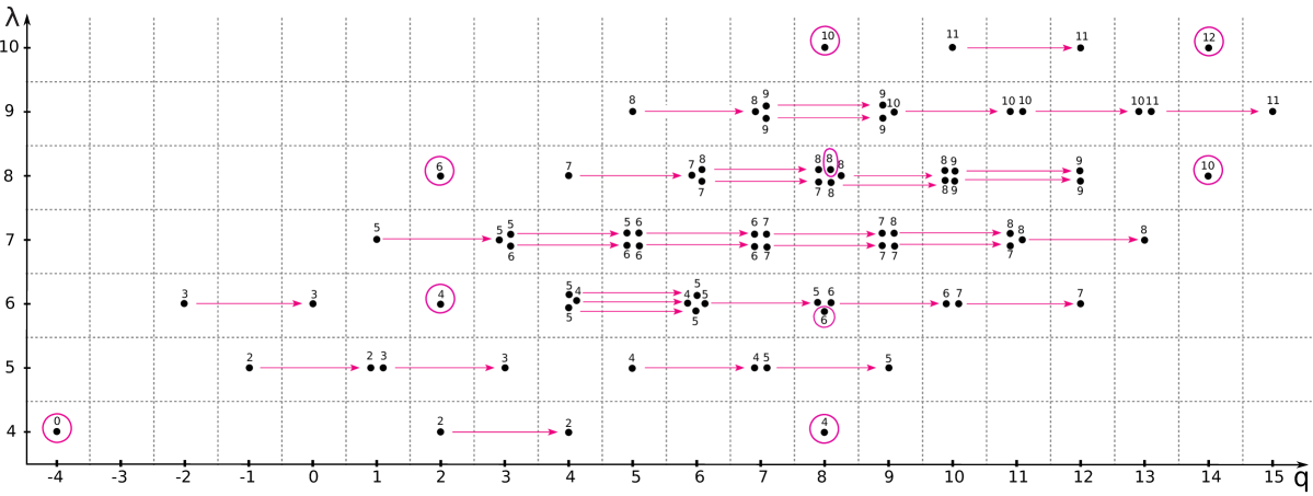
Figure 9: The universal colored differential $d^{\leftarrow}$ acts on the $[2]$-colored Kauffman homology of the trefoil. The dots enclosed by red circles represent the elements in $H_{*}(\mathscr{H}^{{\rm Kauffman}}_{[2]},d^{\leftarrow})$.

In order to isolate the $c=0$ contribution, it was proposed in Marino:2009mw that one has to take into account two sets of Lagrangian branes on $\mathcal{N}_{K,\epsilon}$ and $\mathcal{N}_{K,-\epsilon}$, which are related by the anti-holomorphic involution in the covering geometry. If you deform the conormal bundle $\mathcal{N}_{K}$ to the fiber direction by $\epsilon$, the anti-holomorphic involution creates the two stacks of probe branes $\mathcal{N}_{K,\epsilon}$ and $\mathcal{N}_{K,-\epsilon}=I(\mathcal{N}_{K,\epsilon})$ (See Figure 9 in Marino:2009mw ). Since the $U(N)$ invariants account for the partition function of the covering geometry, the corresponding invariants are described by HOMFLY polynomials $\overline{P}_{(R,S)}(K)$ carrying a composite representation $(R,S)$. Here, the composite representation $(R,S)$ can be considered as a representation with highest weight $\Lambda_{R}+\Lambda_{\overline{S}}$ where $\overline{S}$ is the conjugate representation of $S$. Using this set-up, the $c=0$ contribution in (53) is given by Marino:2009mw

$${\cal F}_{K}^{c=0}(t,g_{s},v)=\log\Big{[}\sum_{R,S}\overline{P}_{(R,S)}(K;\lambda,q)s_{R}(v)s_{S}(v)\Big{]}~{}.$$ (54)

These open-string topological amplitudes can be related to counting degeneracies of M2-M5 bound states in M-theory on the resolved conifold $X$ Gopakumar:1998ii ; Gopakumar:1998jq ; Ooguri:1999bv ; Labastida:2000yw ; Marino:2009mw ; Witten:2011zz , where the configurations of $M$ M5-branes are as follows:

space-time $$: \quad S^{1}\times TN\times X~{},$$ (55)

$$M~{}\text{M5-branes} : \quad S^{1}\times D\times{\mathcal{L}_{K}}~{},$$ (56)

where $D\cong\mathbb{R}^{2}$ is the cigar of the Taub-NUT space $TN\cong\mathbb{R}^{4}$. The M2-branes wrap a two-cycle $\beta\in H_{2}(X,\mathcal{L}_{K})$ of $X$ and end on the stack of the M5-branes. In the orientifold background, a two-cycle can be either an orientable ($c=0$) or a non-orientable ($c=1,2$) Riemann surface of genus $g$ with $h$ boundaries. The boundary condition is specified by the $h$-tuple winding number $w=(w_{1},\cdots,w_{h})$ where the total number $|R|$ of boxes in the Young diagram $R$ for $SU(M)$ is equal to $|R|=\sum_{i=1}^{h}w_{i}$. The Káhler parameter $\lambda$ becomes fugacity for the charge $\beta$ and the variable $z=q-q^{-1}$ corresponds to the fugacity of the charge $g$ in the index which counts M2-M5 bound states. Therefore, one can define the reformulated invariants by the number $\widehat{N}_{R;g,\beta}^{c}(K)$ of the M2-M5 bound states

$$\sum_{g\geq 0}\sum_{\beta\in\mathbb{Z}}\widehat{N}_{R;g,\beta}^{c}(K)z^{2g-1+c}\lambda^{\beta}~{}.$$ (57)

Via the geometric transition, the reformulated invariants can be written in terms of the Chern-Simons invariants of the knot $K$, which is discussed in more detail in Appendix B. Most importantly, since $\widehat{N}_{R;g,\beta}^{c}(K)$ is the number of the M2-M5 bound states, it is conjectured to be an integer Ooguri:1999bv ; Labastida:2000yw ; Marino:2009mw . In Appendix B, we verify this conjecture for the figure-eight with $R=\yng(2)$ or $\yng(1,1)$.

It is conjectured in Gukov:2004hz that the space of the M2-M5 bound states is isomorphic to the knot homologies $\mathscr{H}_{\rm BPS}\cong\mathscr{H}_{\rm knot}$. More precisely, we count the BPS states weighted by the charge $\beta$ as well as the charge $(s,r)$ of the rotation group $U(1)_{q}\times U(1)_{t}$ of the non-compact space $TN\cong\mathbb{R}^{4}$ where the $q$- and $t$-gradings correspond to the equivariant action $U(1)_{q}\times U(1)_{t}$ on the tangent and normal bundle of $D\cong\mathbb{R}^{2}$ in $TN\cong\mathbb{R}^{4}$. With an appropriate change of basis, the space of the BPS states can be identified with the triply-graded homology, so-called Kauffman homology, which categorifies the Kauffman polynomial. The large $N$ duality predicts that the Kauffman homology is isomorphic to $\mathfrak{so}(N)/\mathfrak{sp}(N)$ homology at large $N$ Dunfield:2005si ; Gukov:2005qp . However, when the Kähler parameter $N\sim\log(\lambda)$ varies, the BPS spectrum jumps. Therefore, as argued in Gukov:2011ry , it is anticipated that there exist differentials in the knot homology which capture jumps of the BPS spectrum. In the uncolored case Gukov:2005qp , the structure of the Kauffman homology has been studied. Moreover, it is natural to expect that the colored Kauffman homology incorporates rich differential structure as in colored HOMFLY homology Gukov:2011ry ; Gorsky:2013jxa . Hence, the main goal of this paper is to investigate the differential structure of the colored Kauffman homology.

3.2 B-model description

Mirror symmetry relates the A-model on $M$ to B-model on the mirror manifold $M^{\vee}$. For non-compact toric Calabi-Yau $M$, the mirror manifold $M^{\vee}$ Hori:2000ck is given by

$$uv=H(x,y;a)$$ (58)

where the spectral (holomorphic) curve $H(x,y;a)=0$ with complex structure $a$ can be viewed as the moduli space of the canonical Lagrangian brane Aganagic:2000gs . For instance, the spectral curve for the mirror manifold of the resolved conifold Aganagic:2000gs is expressed by

$$H_{\includegraphics[width=8.5359pt]{unknot}}(x,y;a)=1-ax-y+a^{-1}xy~{},$$ (59)

where the canonical Lagrangian brane wraps the submanifold $\mathcal{L}_{\includegraphics[width=8.5359pt]{unknot}}$ corresponding to the unknot. It was pointed out in Aganagic:2001nx that there is an ambiguity that preserves the geometry of the brane at infinity. It turns out that this corresponds to the mirror geometry for the configuration of the framed unknot ${\raisebox{-1.42271pt}{\includegraphics[width=8.5359pt]{unknot}}}_{f}$, where the spectral curve can be obtained Aganagic:2001nx ; Brini:2011wi by the modular transformation $T^{f}$ of the curve (59)

$$H_{\includegraphics[width=8.5359pt]{unknot}_{f}}(x,y;a)=y^{f}(1-y)+a^{f-1}x(y-a^{2})~{}.$$ (60)

Generalizing this, it was shown in Brini:2011wi that the spectral curve corresponding to the configuration for the torus knot $T_{Q,P}$ can be derived by the $SL(2,\mathbb{Z})$ transformation of the curve (59) as we obtain the Rosso-Jones formula (32):

$$H_{T_{Q,P}}(x,y;a)=y^{P}(1-y)^{Q}+a^{P-Q}x(y-a^{2})^{Q}~{}.$$ (61)

The next step is to understand the mirror geometry of the resolved conifold with the Lagrangian submanifold $\mathcal{L}_{T_{Q,P}}$ for the torus knot $T_{Q,P}$ in the presence of an orientifold. Mirror symmetry maps an anti-holomorphic involution of the A-model into a holomorphic involution of the B-model. The holomorphic involution on the manifold

$${X}^{\vee}=\{(u,v,x,y)\in\mathbb{C}\times\mathbb{C}\times\mathbb{C}^{\times}\times\mathbb{C}^{\times}|uv=H_{\includegraphics[width=8.5359pt]{unknot}}(x,y;a)\}$$ (62)

mirror to the orientifold action on the resolved conifold $X$ was explicitly written in Acharya:2002ag :

$$(u,v,x,y)\to(-u,-ax^{-1}y^{-1}v,x^{-1},a^{2}y^{-1})~{}.$$ (63)

This holomorphic involution can be extended to the geometry $uv=H_{T_{Q,P}}(x,y;a)$ mirror to the resolved conifold with M5-branes wrapping on the Lagrangian submanifold $\mathcal{L}_{T_{Q,P}}$ associated to the torus knot $T_{Q,P}$ in such a way that

$$(u,v,x,y)\to(-u,-a^{P+Q}x^{-1}y^{-(P+Q)}v,x^{-1},a^{2}y^{-1})~{}.$$ (64)

Hence, the geometry mirror to the configuration for the torus knot $T_{Q,P}$ in the presence of an orientifold is $uv=H_{T_{Q,P}}(x,y;a)$ with the involution (64).

On the other hand, in Aganagic:2012jb , the B-model description has been considered in the context of the SYZ formulation Strominger:1996it . Given a Lagrangian brane whose topology is $S^{1}\times\mathbb{R}^{2}$, the moduli space receives the disc instanton corrections depending on the Lagrangian brane. Thus, even with the same resolved conifold background, the disc corrected moduli space of $\mathcal{L}_{K}$ is dependent of a knot $K$. Furthermore, it is conjectured in Aganagic:2012jb that the disc-corrected moduli space of $\mathcal{L}_{K}$ is given by the $a$-deformed $A$-polynomial of $SU$-type for a knot $K$

$$A^{SU}(K;x,y;a)=0~{},$$ (65)

and the corresponding mirror manifold ${X}^{\vee}_{K}$ (58) is expressed as

$$uv=A^{SU}(K;x,y;a)~{}.$$ (66)

The detailed explanation for the $a$-deformed $A$-polynomial of $SU$-type will be given in §6. Note that this conjecture encompasses any knots including non-torus knots.

Although the $a$-deformed $A$-polynomial of $SU$-type for the framed unknot ${\raisebox{-1.42271pt}{\includegraphics[width=8.5359pt]{unknot}}}_{f}$ coincides with the spectral curve $H_{\includegraphics[width=8.5359pt]{unknot}_{f}}(x,y;a)$ given in (60) with suitable change of variables, they are no longer the same for general torus knots. For instance, the spectral curve $H_{T_{2,3}}(x,y;a)=0$ for the trefoil is of genus zero while the zero locus of the $a$-deformed $A$-polynomial of $SU$-type for the trefoil $A^{SU}({\bf 3_{1}};x,y;a)=0$ determines a curve of genus one. Further study has to be undertaken in order to understand the relation between the two descriptions in the case of torus knots. In particular, it is important to study whether the application of the topological recursions Eynard:2007kz to the $a$-deformed $A$-polynomial of $SU$-type $A^{SU}(K;x,y;a)=0$ would provide the large color asymptotic expansion of the colored HOMFLY polynomial $P_{[r]}(K;a,q)$ as done in the case of colored Jones polynomials Dijkgraaf:2010ur ; Borot:2012cw .

Following the generalized SYZ formulation Aganagic:2012jb , it would be easy to conjecture that the disc-corrected moduli space of the Lagrangian brane associated to a knot $K$ in the presence of an orientifold is given by the zero locus of the $\lambda$-deformed $A$-polynomial $A^{SO}(K;x,y;\lambda)$ of $SO$-type. Nevertheless, the authors would like to emphasize that it is desirable to provide some support for the generalized SYZ conjecture Aganagic:2012jb involving a non-trivial knot first in the $SU$ context.

4 Quadruply-graded Kauffman homology

4.1 Review of quadruply-graded HOMFLY homology

In the case of the categorifications, the realization of knot homologies as the space of certain BPS states has given rise to various predictions on the structure of the colored HOMFLY homology. First, it was predicted in Dunfield:2005si that there exists a triply-graded ($(a,q,t)$-graded) HOMFLY homology $(\mathscr{H}^{\rm HOMFLY}_{\yng(1)}(K))_{i,j,k}$, whose graded Euler characteristic is given by the HOMFLY polynomial $P_{\yng(1)}(K;a,q)$. It is endowed with a set of anti-commuting differentials $\{d_{N}\}_{N\in\mathbb{Z}}$ where the homology with respect to $d_{N>0}$ is isomorphic to the $\mathfrak{sl}(N)$ homology Khovanov:2004 , which categorifies the $\mathfrak{sl}(N)$ quantum invariant $P^{\mathfrak{sl}(N)}_{\yng(1)}(K;q)=P_{\yng(1)}(K;a=q^{N},q)$:

$$H_{*}(\mathscr{H}^{\rm HOMFLY}_{\yng(1)}(K),d_{N>0})\cong\mathscr{H}^{\mathfrak{sl}(N)}_{\yng(1)}(K)~{}.$$ (67)

In the sequel, the uncolored triply-graded HOMFLY homology Khovanov:2005 and the differentials $d_{N}$ Rasmussen:2006 were put on mathematically rigorous footing.

In Gukov:2011ry , this approach has been extended to the colored case. Especially, the concrete study has been carried out for the HOMFLY homology carrying the symmetric and anti-symmetric representations. It turns out that the $[r]$-colored ($[1^{r}]$-colored) HOMFLY homology $\mathscr{H}^{\rm HOMFLY}_{[r]}(K)$ ($\mathscr{H}^{\rm HOMFLY}_{[1^{r}]}(K)$) is endowed not only with the $\mathfrak{sl}(N)$ differentials $d_{N}$ but also with the colored differentials $d^{\pm}_{[{r}]\to[{\ell}]}$ ($d^{\pm}_{[{1^{r}}]\to[{1^{\ell}}]}$). The colored differentials descend the original homology to those with lower-rank representations

$$H_{*}(\mathscr{H}^{\rm HOMFLY}_{[r]}(K),d^{\pm}_{[{r}]\to[{\ell}]}) \cong \mathscr{H}^{\rm HOMFLY}_{[\ell]}(K)~{},$$ (68)

$$H_{*}(\mathscr{H}^{\rm HOMFLY}_{[1^{r}]}(K),d^{\pm}_{[{1^{r}}]\to[{1^{\ell}}]}) \cong \mathscr{H}^{\rm HOMFLY}_{[1^{\ell}]}(K)~{},$$ (69)

where $r>\ell\geq 0$. In addition, it was realized in Gukov:2011ry ; Morozov:2012am that the $[r]$-colored HOMFLY homology for certain classes of knots, such as thin knots and torus knots, exhibits the exponential growth property

$$\sum_{i,j,k}a^{i}t^{k}\dim\;(\mathscr{H}^{\rm HOMFLY}_{[r]}(K))_{i,j,k}=\Big{[}\sum_{i,j,k}a^{i}t^{k}\dim\;(\mathscr{H}^{\rm HOMFLY}_{\yng(1)}(K))_{i,j,k}\Big{]}^{r}~{}.$$ (70)

Furthermore, it was conjectured that there exists an isomorphism between $\mathscr{H}^{\rm HOMFLY}_{R}(K)$ and $\mathscr{H}^{\rm HOMFLY}_{R^{t}}(K)$ for an arbitrary representation $R$

$$\phi:(\mathscr{H}^{\rm HOMFLY}_{R}(K))_{i,j,*}\xrightarrow{\cong}(\mathscr{H}^{\rm HOMFLY}_{R^{t}}(K))_{i,-j,*}~{},$$ (71)

Let us note that the representation $R^{t}$ is the transposition of the representation $R$. This involution $\phi$ is called the mirror/transposition symmetry in Gukov:2011ry . Actually, the involution $\phi$ exchanges the positive and negative differentials

$$\phi d_{N}=d_{-N}\phi~{},$$ (72)

when the representation $R$ is either a symmetric or an anti-symmetric representation.

In attempting to elucidate the mirror/transposition symmetry, the two homological gradings denoted by $t_{r}$ and $t_{c}$ are introduced so that colored HOMFLY homology turns into quadruply-graded $(\mathscr{H}^{\rm HOMFLY}_{R}(K))_{i,j,k,\ell}$: $(a,q,t_{r},t_{c})$-gradings Gorsky:2013jxa . Particularly, to every generator $x$ of the $[r]$-colored quadruply-graded HOMFLY homology, one can associate a $\delta$-grading by

$$\delta(x):=a(x)+\frac{q(x)}{2}-\frac{t_{r}(x)+t_{c}(x)}{2}~{}.$$ (73)

Although the four gradings are independent in general, a knot $K$ is called homologically-thin if all generators of $\mathscr{H}^{\rm HOMFLY}_{[r]}(K)$ have the same $\delta$-grading which is equal to $\frac{r}{2}S(K)$ where we denote the $S$-invariant of the knot $K$ by $S(K)$ Rasmussen:2004 . Moreover, it became apparent that all of the structural properties and isomorphisms become particularly elegant with the introduction of the $Q$-grading defined by

$$Q(x):=\frac{q(x)+t_{r}(x)-t_{c}(x)}{\rho}~{}.$$ (74)

when the representation is specified by a rectangular Young diagram $[r^{\rho}]$. While it is just a regrading of $(\mathscr{H}^{\rm HOMFLY}_{[r^{\rho}]}(K))_{i,j,k,\ell}$, it is named the tilde-version of colored HOMFLY homology $\widetilde{}\mathscr{H}^{\rm HOMFLY}_{[r^{\rho}]}(K)$ due to its importance:

$$(\widetilde{}\mathscr{H}^{\rm HOMFLY}_{[r^{\rho}]}(K))_{i,j,k,l}\;:=\;(\mathscr{H}^{\rm HOMFLY}_{[r^{\rho}]}(K))_{i,\rho j-k+l,k,l}~{}.$$ (75)

It is the uncolored case only when the two $t$-gradings coincide and therefore the resulting homology is triply-graded in agreement with Dunfield:2005si . It simply follows from (74) that the $q$- and $Q$-gradings of the uncolored homology are the same.

The definite advantage of the quadruply-graded theory is that it makes all of the structural features and isomorphisms completely explicit. To see them, let us define the Poincaré polynomial of the quadruply-graded homology:

$$\mathscr{P}_{[r^{\rho}]}(K;a,q,t_{r},t_{c}) := \sum_{i,j,k,\ell}a^{i}q^{j}t_{r}^{k}t_{c}^{\ell}~{}\dim\;(\mathscr{H}^{\rm HOMFLY}_{[r^{\rho}]}(K))_{i,j,k,\ell}~{},$$ (76)

$$\widetilde{}\mathscr{P}_{[r^{\rho}]}(K;a,Q,t_{r},t_{c}) := \sum_{i,j,k,\ell}a^{i}Q^{j}t_{r}^{k}t_{c}^{\ell}~{}\dim\;(\widetilde{}\mathscr{H}^{\rm HOMFLY}_{[r^{\rho}]}(K))_{i,j,k,\ell}~{},$$ (77)

where they are related by

$$\widetilde{}\mathscr{P}_{[r^{\rho}]}(K;a,q^{\rho},t_{r}q^{-1},t_{c}q)=\mathscr{P}_{[r^{\rho}]}(K;a,q,t_{r},t_{c})~{}.$$ (78)

Now, let us briefly describe the structural properties of the quadruply-graded colored HOMFLY homology. We refer the reader to Gorsky:2013jxa for more detail.

• Self-symmetry (Conjecture 3.1 Gorsky:2013jxa )
  Once we use the tilde-version of the colored HOMFLY homology, a new symmetry in $\widetilde{}\mathscr{H}^{{\rm HOMFLY}}_{[r^{\rho}]}(K)$ becomes manifest:

  $$(\widetilde{}\mathscr{H}^{{\rm HOMFLY}}_{[r^{\rho}]}(K))_{i,j,k,\ell} \cong (\widetilde{}\mathscr{H}^{{\rm HOMFLY}}_{[r^{\rho}]}(K))_{i,-j,k-\rho j,\ell-rj}~{},$$ (79)

  which can be stated at the level of the Poincaré polynomial

  $$\widetilde{}\mathscr{P}_{[r^{\rho}]}(K;a,Q,t_{r},t_{c}) = \widetilde{}\mathscr{P}_{[r^{\rho}]}(K;a,Q^{-1}t_{r}^{-\rho}t_{c}^{-r},t_{r},t_{c})~{}.$$ (80)

• Mirror/Transposition symmetry (Conjecture 3.3 and 3.4 Gorsky:2013jxa )
  The $[\rho^{r}]$-colored quadruply-graded HOMFLY homology enjoys the mirror/transposition symmetry

  $$(\widetilde{}\mathscr{H}^{{\rm HOMFLY}}_{[\rho^{r}]}(K))_{i,j,k,\ell}\cong(\widetilde{}\mathscr{H}^{{\rm HOMFLY}}_{[r^{\rho}]}(K))_{i,j,\ell,k}\cong(\widetilde{}\mathscr{H}^{{\rm HOMFLY}}_{[r^{\rho}]}(K))_{i,-j,\ell-\rho j,k-rj}~{},~{}~{}~{}~{}~{}$$ (81)

  which can be expressed in terms of the Poincaré polynomial

  $$\widetilde{}\mathscr{P}_{[\rho^{r}]}(K;a,Q,t_{r},t_{c}) = \widetilde{}\mathscr{P}_{[r^{\rho}]}(K;a,Q,t_{c},t_{r})=\widetilde{}\mathscr{P}_{[r^{\rho}]}(K;a,Q^{-1}t_{c}^{-\rho}t_{r}^{-r},t_{c},t_{r})~{}.~{}~{}~{}~{}$$ (82)

  This lifts the following relation between the colored HOMFLY polynomials

  $$P_{R^{t}}(K;a,q)=P_{R}(K;a,-q^{-1})=P_{R}(K;-a,q^{-1})~{},$$ (83)

  for any representation $R$.

• Refined exponential growth property (Conjecture 3.8 and 3.9 Gorsky:2013jxa )
  Let $K$ be either a thin knot or a torus knot. The $[r^{\rho}]$-colored quadruply-graded HOMFLY homology of the knot $K$ obeys the refined exponential growth property

  $$\widetilde{}\mathscr{P}_{[r^{\rho}]}(K;a,Q,t_{r},t_{c}=1) = \left[\widetilde{}\mathscr{P}_{[1^{\rho}]}(K;a,Q,t_{r},t_{c}=1)\right]^{r}~{},$$ (84)

  $$\widetilde{}\mathscr{P}_{[r^{\rho}]}(K;a,Q,t_{r}=1,t_{c}) = \left[\widetilde{}\mathscr{P}_{[r]}(K;a,Q,t_{r}=1,t_{c})\right]^{\rho}~{}.$$ (85)

  It follows immediately that

  $$\dim\mathscr{H}^{\rm HOMFLY}_{[r^{\rho}]}(K)=\left[\dim\mathscr{H}^{\rm HOMFLY}_{\yng(1)}(K)\right]^{r\rho}~{}.$$ (86)

  The analogous statement at the polynomial level is as follows. For any knot $K$ and an arbitrary representation $R$, the following identity holds DuninBarkowski:2011yx :

  $$P_{R}(K;a,q=1)=\left[P_{\yng(1)}(K;a,q=1)\right]^{|R|}~{},$$ (87)

  where $|R|$ is the total number of the Young diagram corresponding to the representation $R$.

• $\mathfrak{sl}(n|m)$ differentials
  It was proposed in Gorsky:2013jxa that the colored HOMFLY homology is actually gifted with a collection of the differentials $\{d_{n|m}\}$ labeled by two non-negative integers $(n,m)$ associated to the Lie superalgebra $\mathfrak{sl}(n|m)$. These are generalizations of the differentials $\{d_{N}\}$ (67). It appears that the representation theory of $\mathfrak{sl}(n|m)$ explains the behavior of the colored differentials. In this paper, we will not go into the detail about the $\mathfrak{sl}(n|m)$ differentials.

• Colored differentials
  For each rectangular Young diagram $[r^{\rho}]$, one can define colored differentials that remove any number of columns or rows from the original Young diagram $[r^{\rho}]$. For every $\ell$ with $r>\ell\geq 0$, there are two different column-removing differentials $d^{\pm}_{[r^{\rho}]\to[\ell^{\rho}]}$, and for every $\sigma$ with $\rho>\sigma\geq 0$, there are two different row-removing differentials $d^{\pm}_{[r^{\rho}]\to[r^{\sigma}]}$ on $\widetilde{}\mathscr{H}^{\rm HOMFLY}_{[r^{\rho}]}(K)$. These are generalizations of (68):

  $$H_{*}(\widetilde{}\mathscr{H}^{\rm HOMFLY}_{[r^{\rho}]}(K),d^{\pm}_{[{r^{\rho}}]\to[{\ell^{\rho}}]}) \cong \widetilde{}\mathscr{H}^{\rm HOMFLY}_{[\ell^{\rho}]}(K)~{},$$ (88)

  $$H_{*}(\widetilde{}\mathscr{H}^{\rm HOMFLY}_{[r^{\rho}]}(K),d^{\pm}_{[{r^{\rho}}]\to[{r^{\sigma}}]}) \cong \widetilde{}\mathscr{H}^{\rm HOMFLY}_{[r^{\sigma}]}(K)~{}.$$ (89)

  The isomorphisms above involve regrading. One of the striking features of the quadruply-graded homology is that it makes the regrading very explicit.

• Universal colored differentials
  If the representation is specified either by $[r,r]$ or by $[2^{r}]$, there exists yet another set of colored differentials $d^{\uparrow}$ or $d^{\leftarrow}$ so that

  $$H_{*}(\widetilde{}\mathscr{H}^{\rm HOMFLY}_{[r,r]}(K),d^{\uparrow}) \cong \widetilde{}\mathscr{H}^{\rm HOMFLY}_{[r]}(K)~{},$$ (90)

  $$H_{*}(\widetilde{}\mathscr{H}^{\rm HOMFLY}_{[2^{r}]}(K),d^{\leftarrow}) \cong \widetilde{}\mathscr{H}^{\rm HOMFLY}_{[1^{r}]}(K)~{}.$$ (91)

  They are called universal colored differentials because they are universal in the sense that their $a$-degree is equal to $0$.

4.2 Properties of quadruply-graded Kauffman homology

Let us now discuss about the categorifications of Kauffman polynomials. The properties of the triply-graded homology that categorifies the uncolored Kauffman polynomials have been investigated in Gukov:2005qp ; Khovanov:2007 . Like HOMFLY homology, it is gifted with a collection of the differentials $\{d_{N}\}_{N\in\mathbb{Z}}$ so that the homology with respect to the differential $d_{N>1}$ is isomorphic to the $\mathfrak{so}(N)$ homology, while the homology with respect to the differential $d_{N<0}$ is isomorphic to the $\mathfrak{sp}(N)$ homology. Furthermore, it was found in Gukov:2005qp through the analysis of the Landau-Ginzburg theory that the most characteristic property of the Kauffman homology is that it contains the HOMFLY homology. More precisely, it is endowed with the so-called universal differential $d_{\hbox to0.0pt{\raise 1.2pt\hbox{$\scriptstyle\rightarrow$}\hss}\lower 1.2pt\hbox{$\scriptstyle\leftarrow$}}^{\rm univ}$ whose homology is isomorphic with the HOMFLY homology:

$$H_{*}(\mathscr{H}^{\rm Kauffman}_{\yng(1)}(K),d_{\hbox to0.0pt{\raise 1.2pt\hbox{$\scriptstyle\rightarrow$}\hss}\lower 1.2pt\hbox{$\scriptstyle\leftarrow$}}^{\rm univ})\cong\mathscr{H}^{\rm HOMFLY}_{\yng(1)}(K)~{}.$$ (92)

From the perspective of topological string theory, it is natural to think that there exists the triply-graded homology theory categorifying Kauffman polynomials colored by arbitrary representations. Especially, it is expected that the structure becomes clear if we use quadruple-gradings, as in the case of colored HOMFLY homology, when the colors are specified by rectangular Young tableaux. Hence, our goal in this section is to clarify all the structural features and isomorphisms in the colored quadruply-graded Kauffman homology.

As we have seen in §2.2, for any representation $R$, there is the $R$-colored reduced Kauffman polynomial $F_{R}(K;\lambda,q)$ of a knot $K$. We conjecture the existence of the finite-dimensional homology $\mathscr{H}^{\rm Kauffman}_{R}(K)$ of a knot $K$ categorifying the $R$-colored reduced Kauffman polynomial $F_{R}(K;\lambda,q)$ of the knot $K$. In this paper, we focus on the case that the representation $R$ is specified by a rectangular Young tableau $[r^{\rho}]$. In this case, we further conjecture that the $[r^{\rho}]$-colored Kauffman homology $(\mathscr{H}^{\rm Kauffman}_{[r^{\rho}]}(K))_{i,j,k,\ell}$ of a knot $K$ is quadruply-graded so that its Poincaré polynomial,

$$\mathscr{F}_{[r^{\rho}]}(K;\lambda,q,t_{r},t_{c}) := \sum_{i,j,k,\ell}\lambda^{i}q^{j}t_{r}^{k}t_{c}^{\ell}~{}\dim\;(\mathscr{H}^{\rm Kauffman}_{[r^{\rho}]}(K))_{i,j,k,\ell}~{},$$ (93)

reduces to the $[r^{\rho}]$-colored Kauffman polynomial in the following way:

$$\mathscr{F}_{[r^{\rho}]}(K;\lambda,q,t_{r}=-1,t_{c}=1)=\mathscr{F}_{[r^{\rho}]}(K;\lambda,q,t_{r}=1,t_{c}=-1)=F_{[r^{\rho}]}(K;\lambda,q)~{}.$$ (94)

As in the case of the HOMFLY homology, one can associate a $\delta$-grading to every generator $x$ of the $[r]$-colored quadruply-graded Kauffman homology by

$$\delta(x):=\frac{3\lambda(x)}{2}+\frac{q(x)}{2}-\frac{t_{r}(x)+t_{c}(x)}{2}~{}.$$ (95)

For a homologically-thin knot $K_{\rm thin}$, the $\delta$-gradings of all the generators are equal to $r\,S(K_{\rm thin})$. In addition, by introducing the $Q$-grading (74), we define the tilde-version of the $[r^{\rho}]$-colored quadruply-graded Kauffman homology

$$(\widetilde{}\mathscr{H}_{[r^{\rho}]}^{{\rm Kauffman}}(K))_{i,j,k,\ell}:=(\mathscr{H}_{[r^{\rho}]}^{{\rm Kauffman}}(K))_{i,\rho j-k+\ell,k,\ell}~{},$$ (96)

and its Poincaré polynomial

$$\widetilde{}\mathscr{F}_{R}(K;\lambda,Q,t_{r},t_{c}):=\sum_{i,j,k,\ell}\lambda^{i}Q^{j}t_{r}^{k}t_{c}^{\ell}~{}\dim\;(\widetilde{}\mathscr{H}^{\rm Kauffman}_{R}(K))_{i,j,k,\ell}~{}.$$ (97)

In terms of the Poincaré polynomials, the relation (96) can be rephrased by

$$\widetilde{}\mathscr{F}_{[r^{\rho}]}(K;\lambda,q^{\rho},t_{r}q^{-1},t_{c}q)=\mathscr{F}_{[r^{\rho}]}(K;\lambda,q,t_{r},t_{c})~{}.$$ (98)

It is the uncolored case only when the two $t$-gradings coincide and therefore the resulting homology is triply-graded in agreement with Gukov:2005qp . It clearly follows from (74) that the $q$- and $Q$-gradings of the uncolored homology are the same.

In what follows, we conjecture the structural properties of the $[r^{\rho}]$-colored Kauffman homology. Although they are very similar, we predict that there are two differences between the $[r^{\rho}]$-colored Kauffman homology and the $[r^{\rho}]$-colored HOMFLY homology. One of the difference is that the $[r^{\rho}]$-colored Kauffman homology does not enjoy the self-symmetry. The other is that there are differentials which relate the $[r]$-colored Kauffman homology to the $[r]$-colored HOMFLY homology.

• Mirror/Transposition symmetry
  The $[r^{\rho}]$-colored Kauffman homology enjoys mirror/transposition symmetry

  $$(\widetilde{}\mathscr{H}^{{\rm Kauffman}}_{[\rho^{r}]}(K))_{i,j,k,\ell} \cong (\widetilde{}\mathscr{H}^{{\rm Kauffman}}_{[r^{\rho}]}(K))_{i,-j,\ell-\rho j,k-rj}~{},$$ (99)

  which can be rephrased in terms of the Poincaré polynomial

  $$\widetilde{}\mathscr{F}_{[\rho^{r}]}(K;\lambda,Q,t_{r},t_{c}) = \widetilde{}\mathscr{F}_{[r^{\rho}]}(K;\lambda,Q^{-1}t_{c}^{-\rho}t_{r}^{-r},t_{c},t_{r})~{}.$$ (100)

  At the decategorified level, for any representation $R$, there is the comparable symmetry between the $R$-colored and the $R^{t}$-colored Kauffman polynomial

  $$F_{R^{t}}(K;\lambda,q)=F_{R}(K;-\lambda,q^{-1})=F_{R}(K;\lambda,-q^{-1})~{}.$$ (101)

  Only in the uncolored case can the mirror/transposition symmetry be regarded as the self-symmetry.

• Refined exponential growth property
  Let $K$ be a thin knot or a torus knot. Then, the Kauffman homology carrying a rectangular Young tableau possesses the refined exponential growth property

  $$\widetilde{}\mathscr{F}_{[r^{\rho}]}(K;\lambda,Q,t_{r},t_{c}=1) = \left[\widetilde{}\mathscr{F}_{[1^{\rho}]}(K;\lambda,Q,t_{r},t_{c}=1)\right]^{r}~{},$$ (102)

  $$\widetilde{}\mathscr{F}_{[r^{\rho}]}(K;\lambda,Q,t_{r}=1,t_{c}) = \left[\widetilde{}\mathscr{F}_{[r]}(K;\lambda,Q,t_{r}=1,t_{c})\right]^{\rho}~{}.$$ (103)

  The analogous statement at the polynomial level is as follows. For any knot $K$ and an arbitrary representation $R$, the following identity holds:

  $$F_{R}(K;a,q=1)=\left[F_{\yng(1)}(K;a,q=1)\right]^{|R|}~{}.$$ (104)

• $\mathfrak{so}/\mathfrak{sp}$ differentials
  The colored Kauffman homology is gifted with a set of the differentials $d_{N}$ so that the homology of $\mathscr{H}^{\rm Kauffman}_{R}(K)$ with respect to $d_{N}$ is isomorphic either to the $\mathfrak{so}(N)$ homology carrying the representation $R$ for $N\geq 2$ or to the $\mathfrak{sp}(N)$ homology carrying the representation $R^{t}$ for $N\leq-2$

  $$H_{*}(\mathscr{H}^{\rm Kauffman}_{R}(K),d_{N})\cong\left\{\begin{array}[]{ll}\mathscr{H}^{\mathfrak{so}(N)}_{R}&(N\geq 2)\\ \mathscr{H}^{\mathfrak{sp}(-N)}_{R^{t}}&(N\leq-2)\end{array}\right.~{}.$$ (107)

• Universal differentials
  The $[r^{\rho}]$-colored Kauffman homology is endowed with the universal differential $d^{\rm univ}$ so that the homology with respect to the universal differential is isomorphic to the $[r^{\rho}]$-colored HOMFLY homology

  $$H_{*}(\widetilde{}\mathscr{H}^{\rm Kauffman}_{[r^{\rho}]}(K),d^{\rm univ}) \cong \widetilde{}\mathscr{H}^{\rm HOMFLY}_{[r^{\rho}]}(K)~{}.$$ (108)

  They are universal in the sense that their $\lambda$-degree is equal to $0$.

• Diagonal differentials
  We conjecture the existence of other differentials whose homologies in the $[r^{\rho}]$-colored Kauffman homology are isomorphic to the $[r^{\rho}]$-colored HOMFLY homology. We call them diagonal differentials, $d^{\pm}_{\rm diag}$, so that

  $$H_{*}(\widetilde{}\mathscr{H}^{\rm Kauffman}_{[r^{\rho}]}(K),d^{\pm}_{\rm diag}) \cong \widetilde{}\mathscr{H}^{\rm HOMFLY}_{[r^{\rho}]}(K)~{}.$$ (109)

  They are not universal since their $\lambda$-degree is equal to $-1$. They are diagonal in the sense that every generator $x\in H_{*}(\widetilde{}\mathscr{H}^{\rm Kauffman}_{[r^{\rho}]}(K),d^{\pm}_{\rm diag})$ obeys the grading relation

  $$\lambda(x)\mp Q(x)=r\;S(K)~{}.$$ (110)

• Colored differentials
  There exists a collection of colored differentials that send the colored Kauffman homology to those with the lower-rank representations.

  $$H_{*}(\widetilde{}\mathscr{H}^{\rm Kauffman}_{[r^{\rho}]}(K),d^{\pm}_{[r^{\rho}]\to[\ell^{\rho}]}) \cong \widetilde{}\mathscr{H}^{\rm Kauffman}_{[\ell^{\rho}]}(K)~{},$$ (111)

  $$H_{*}(\widetilde{}\mathscr{H}^{\rm Kauffman}_{[r^{\rho}]}(K),d^{\pm}_{[r^{\rho}]\to[r^{\sigma}]}) \cong \widetilde{}\mathscr{H}^{\rm Kauffman}_{[r^{\sigma}]}(K)~{}.$$ (112)

  It should be stressed that the existence of the colored differentials becomes manifest only when we use the tilde-version of the colored Kauffman homology.

• Universal colored differentials
  If the representation is specified either by $[r,r]$ or by $[2^{r}]$, there exists yet another set of colored differentials $d^{\uparrow}$ or $d^{\leftarrow}$ so that

  $$H_{*}(\widetilde{}\mathscr{H}^{\rm Kauffman}_{[r,r]}(K),d^{\uparrow}) \cong \widetilde{}\mathscr{H}^{\rm Kauffman}_{[r]}(K)~{},$$ (113)

  $$H_{*}(\widetilde{}\mathscr{H}^{\rm Kauffman}_{[2^{r}]}(K),d^{\leftarrow}) \cong \widetilde{}\mathscr{H}^{\rm Kauffman}_{[1^{r}]}(K)~{}.$$ (114)

  They are called universal colored differentials because they are universal in the sense that their $\lambda$-degree is equal to $0$.

In the following subsections, we shall explicate all the differentials in detail. Since the size of the colored Kauffman homology is too large for concrete study of arbitrary rectangular Young tableaux, we restrict ourselves to the case that the representations are specified by the Young tableaux $[r]$ and their transpositions $[1^{r}]$.

Before moving on to the next subsection, let us define the Poincaré polynomial of the homology with respect to a differential $d$ in the HOMFLY homology

$$\mathscr{P}(\mathscr{H}^{\rm HOMFLY}_{R}(K),d)(a,q,t_{r},t_{c}) := \sum_{i,j,k,\ell}a^{i}q^{j}t_{r}^{k}t_{c}^{\ell}~{}\dim H_{*}(\mathscr{H}^{\rm HOMFLY}_{R}(K),d)_{i,j,k,\ell}~{},$$ (115)

$$\widetilde{}\mathscr{P}(\widetilde{}\mathscr{H}^{\rm HOMFLY}_{R}(K),d)(a,Q,t_{r},t_{c}) := \sum_{i,j,k,\ell}a^{i}Q^{j}t_{r}^{k}t_{c}^{\ell}~{}\dim H_{*}(\widetilde{}\mathscr{H}^{\rm HOMFLY}_{R}(K),d)_{i,j,k,\ell}~{},~{}~{}~{}~{}~{}~{}~{}~{}~{}$$ (116)

and the Poincaré polynomial of the homology with respect to a differential $d$ in the Kauffman homology

$$\widetilde{}\mathscr{F}(\widetilde{}\mathscr{H}^{\rm Kauffman}_{R}(K),d)(\lambda,Q,t_{r},t_{c}) := \sum_{i,j,k,\ell}\lambda^{i}Q^{j}t_{r}^{k}t_{c}^{\ell}~{}\dim H_{*}(\widetilde{}\mathscr{H}^{\rm Kauffman}_{R}(K),d)_{i,j,k,\ell}~{},$$ (117)

$$\mathscr{F}(\mathscr{H}^{\rm Kauffman}_{R}(K),d)(\lambda,q,t_{r},t_{c}) := \sum_{i,j,k,\ell}\lambda^{i}q^{j}t_{r}^{k}t_{c}^{\ell}~{}\dim H_{*}(\mathscr{H}^{\rm Kauffman}_{R}(K),d)_{i,j,k,\ell}~{}.~{}~{}~{}~{}~{}~{}~{}~{}~{}~{}$$ (118)

4.3 $\mathfrak{so}/\mathfrak{sp}$ differentials

There is a set of the differentials $\{d_{N}\}_{N\in\mathbb{Z}}$ inherent in the colored Kauffman homology so that the homology with respect to $d_{N}$ is isomorphic to the colored $\mathfrak{so}/\mathfrak{sp}$ homology (107). To see the isomorphism (107) explicitly, it is convenient to use the Poincaré polynomials in the $(\lambda,q,t_{r},t_{c})$-gradings. Specifically, in the case of the $[r]$-colored Kauffman homology, we have the following identities at the level of the Poincaré polynomials

$$\mathscr{F}(\mathscr{H}^{\rm Kauffman}_{[r]}(K),d_{N})(\lambda=q^{N-1},q,t,1)=\left\{\begin{array}[]{ll}\mathscr{P}^{{\mathfrak{so}}(N)}_{[r]}(K;q,t)&(N\geq 2)\\ t^{rS(K)}\mathscr{P}^{{\mathfrak{sp}}(-N)}_{[1^{r}]}(K;q^{-1},t)&(N\leq-2r)\end{array}\right.,~{}~{}~{}~{}$$ (121)

where the $(\lambda,q,t_{r},t_{c})$-degrees of the differential $d_{N}$ acting on $\mathscr{H}^{\rm Kauffman}_{[r]}(K)$ are

$$\deg d_{N}\Big{|}_{\mathscr{H}^{\rm Kauffman}_{[r]}(K)}=\left\{\begin{array}[]{ll}(-1,N-1,-1,*)&(N\geq 2)\\ (-1,N-1,N-1,*)&(N\leq-2r)\end{array}\right.~{}.$$ (124)

The differential $d_{-2}$, which specializes the uncolored Kauffman homology to the $\mathfrak{sp}(2)$ homology, acts nontrivially even on the Kauffman homology of a thin knot Gukov:2005qp ; Gukov:2011ry .

On the other hand, the $(\lambda,q,t_{r},t_{c})$-degrees of the differential $d_{N}$ acting on $\mathscr{H}^{\rm Kauffman}_{[1^{r}]}(K)$ are

$$\deg d_{N}\Big{|}_{\mathscr{H}^{\rm Kauffman}_{[1^{r}]}(K)}=\left\{\begin{array}[]{ll}(-1,N-1,*,-1)&(N\geq r+2)\\ (-1,N-1,*,N-1)&(N\leq-2)\end{array}\right.~{},$$ (127)

so that we can see the isomorphism (107) in terms of the Poincaré polynomials in the following way:

$$\mathscr{F}(\mathscr{H}^{\rm Kauffman}_{[1^{r}]}(K),d_{N})(\lambda=q^{N-1},q,t,1)=\left\{\begin{array}[]{ll}\mathscr{P}^{{\mathfrak{so}}(N)}_{[1^{r}]}(K;q,t)&(N\geq r+2)\\ t^{rS(K)}\mathscr{P}^{{\mathfrak{sp}}(-N)}_{[r]}(K;q^{-1},t)&(N\leq-2)\end{array}\right..~{}~{}~{}~{}~{}~{}$$ (130)

4.4 Relations from representation theory

The $\mathfrak{so}/\mathfrak{sp}$ specializations by using the differentials $d_{N}$ are useful to determine the colored Kauffman homology. In fact, there are several isomorphisms of representations which lead to nontrivial identities among the homological invariants.

• It is well-known that the vector representation $\yng(1)$ of $\mathfrak{so}(3)$ is isomorphic to the spin-1 representation $\yng(2)$ of $\mathfrak{sl}(2)$. Moreover, since this relation can be extended to the symmetric product

  $$(\mathfrak{so}(3),[r])\cong(\mathfrak{sl}(2),[2r])~{},$$ (131)

  we have the isomorphism between the $[r]$-colored $\mathfrak{so}(3)$ homology and the $[2r]$-colored $\mathfrak{sl}(2)$ homology in the $t_{r}$-grading

  $$\mathscr{F}(\mathscr{H}^{{\rm Kauffman}}_{[r]}(K),d_{3})(\lambda=q^{2},q,t_{r},t_{c}=1)$$ (132)

  $$\hskip 56.9055pt=\mathscr{P}(\mathscr{H}^{{\rm HOMFLY}}_{[2r]}(K),d_{2})(a=q,q^{1/2},t_{r},t_{c}=1)~{}.$$ (133)

  Particularly, since the differentials act trivially for a thin knot $K_{\rm thin}$, the naive substitutions lead to the identity

  $$\mathscr{F}_{[r]}(K_{\rm thin};q^{2},q,t_{r},1)=\mathscr{P}_{[2r]}(K_{\rm thin};q,q^{1/2},t_{r},1)~{}.$$ (134)

• In addition, since $\mathfrak{so}(4)$ is isomorphic to $\mathfrak{sl}(2)\oplus\mathfrak{sl}(2)$ as Lie algebras, we have

  $$\mathscr{F}(\mathscr{H}^{{\rm Kauffman}}_{[r]}(K),d_{4})(\lambda=q^{3},q,t_{r},t_{c}=1)$$ (135)

  $$\hskip 56.9055pt=\left[\mathscr{P}(\mathscr{H}^{{\rm HOMFLY}}_{[r]}(K),d_{2})(a=q^{2},q,t_{r},t_{c}=1)\right]^{2}~{}.$$ (136)

  In particular, for a thin knot $K_{\rm thin}$, the identity holds even with the $t_{c}$-gradings

  $$\mathscr{F}_{[r]}(K_{\rm thin};q^{3},q,t_{r},t_{c})=\left[\mathscr{P}_{[r]}(K_{\rm thin};q^{2},q,t_{r},t_{c})\right]^{2}~{}.$$ (137)

• The isomorphism between $\mathfrak{sp}(2)$ and $\mathfrak{sl}(2)$ leads to

  $$\mathscr{F}(\mathscr{H}^{{\rm Kauffman}}_{[1^{r}]}(K),d_{-2})(\lambda=q^{3},q^{-1},1,t)$$ (138)

  $$\hskip 85.35826pt=t^{rS(K)}\mathscr{P}(\mathscr{H}^{{\rm HOMFLY}}_{[r]}(K),d_{2})(a=q^{4},q^{2},t,1)~{}.$$ (139)

  Moreover, the differential $d_{-2}$ can be evident in the $(\lambda,Q,t_{r},t_{c})$-grading whose degree is $(-1,-3,-3r,-3)$ on $\widetilde{}\mathscr{H}_{[1^{r}]}^{\rm Kauffman}(K_{\rm thin})$. We predict that the Poincaré polynomial of the homology $H_{*}(\widetilde{}\mathscr{H}^{\rm Kauffman}_{[1^{r}]}(K),d_{-2})$ with respect to the differential $d_{-2}$ can be expressed in terms of the $[r]$-colored HOMFLY homology

  $$\widetilde{}\mathscr{F}(\widetilde{}\mathscr{H}^{{\rm Kauffman}}_{[1^{r}]}(K_{\rm thin}),d_{-2})(\lambda,Q,t_{r},t_{c})$$ (140)

  $$=\lambda^{\frac{rS(K)}{2}}Q^{\frac{3rS(K)}{2}}t_{r}^{\frac{r(3r-1)S(K)}{2}}t_{c}^{rS(K)}\widetilde{}\mathscr{P}_{[r]}(K_{\rm thin};\lambda Q^{-1}t_{r}^{1-r},(\lambda Q^{-1}t_{r}^{1-r})^{\frac{1}{2}},t_{r}^{-1}t_{c},t_{r}^{2})~{}.$$

• Furthermore, the isomorphism of the representations,

  $$(\mathfrak{so}(6),[r])\cong(\mathfrak{sl}(4),[r,r])~{},$$ (141)

  provides us with the isomorphism between the $[r]$-colored $\mathfrak{so}(6)$ homology and the $[r,r]$-colored $\mathfrak{sl}(4)$ homology in the $t_{c}$-grading

  $$\mathscr{F}(\mathscr{H}^{{\rm Kauffman}}_{[r]}(K),d_{6})(\lambda=q^{5},q,t_{r}=1,t_{c})$$ (142)

  $$\hskip 71.13188pt=\mathscr{P}(\mathscr{H}^{{\rm HOMFLY}}_{[r,r]}(K),d_{4})(a=q^{4},q,t_{r}=1,t_{c})~{}.$$ (143)

  Specifically for a thin knot $K_{\rm thin}$, we have the following relation:

  $$\mathscr{F}_{[r]}(K_{\rm thin};q^{5},q,1,t_{c})=\mathscr{P}_{[r,r]}(K_{\rm thin};q^{4},q^{2},1,t_{c})~{}.$$ (144)

  Interestingly, the relation (142) from representation theory sheds new light on the structure of the $[r]$-colored Kauffman homology. In fact, the relation (142) implies that the differential structure of $\mathscr{H}^{\mathfrak{sl}(4)}_{[r,r]}(K)$ can be mapped to that of $\mathscr{H}^{\mathfrak{so}(6)}_{[r]}(K)$. Furthermore, the $[r]$-colored Kauffman homology of a thin knot is expected to have a similar differential structure to the $[r,r]$-colored HOMFLY homology because there is a one-to-one correspondence between the generators of both the homologies through (144). Actually, in the $[r]$-colored Kauffman homology, one can find the counterparts of all the colored differentials inherent in the $[r,r]$-colored HOMFLY homology. This can be seen in Table 1, where the differentials are related by

  $$(5\lambda+Q-t_{r}+t_{c})[d^{\rm Kauffman}]=\pm(4a+2Q-t_{r}+t_{c})[d^{\rm HOMFLY}]~{},$$ (145)

  with the same $t_{c}$-degrees $t_{c}[d^{\rm Kauffman}]=t_{c}[d^{\rm HOMFLY}]$ since (144) can be written in terms of the tilde-version

  $$\widetilde{}\mathscr{F}_{[r]}(K_{\rm thin};\lambda=q^{5},Q=q,t_{r}=q^{-1},t_{c}=qt)$$ (146)

  $$\hskip 85.35826pt=\widetilde{}\mathscr{P}_{[r,r]}(K_{\rm thin};a=q^{4},Q=q^{2},t_{r}=q^{-1},t_{c}=qt)~{}.$$ (147)

$\widetilde{}\mathscr{H}^{\rm Kauffman}_{[r]}$(K)		$\widetilde{}\mathscr{H}^{\rm HOMFLY}_{[r,r]}$(K)
differentials	$(\lambda,Q,t_{r},t_{c})$-degrees	differentials	$(a,Q,t_{r},t_{c})$-degrees
$d^{\rm univ}_{\to}$	$(0,2,1,1)$	$d^{+}_{[r,r]\to[r]}$	$(-2,2,-3,-1)$
$d^{-}_{\rm diag}$	$(-1,-3,-3,-2r-1)$	$d^{-}_{[r,r]\to[r]}$	$(-2,-2,-7,-2r-1)$
$d_{[r]\to[\ell]}^{+}$	$(-1,1,-1,-2\ell-1)$	$d^{+}_{[r,r]\to[\ell,\ell]}$	$(-2,2,-1,-2\ell-1)$
$d_{[r]\to[\ell]}^{-}$	$(-2,0,-3,-2\ell-2r-1)$	$d^{-}_{[r,r]\to[\ell,\ell]}$	$(-2,-2,-5,-2\ell-2r-1)$
$d^{\leftarrow}\ (r=2)$	$(0,0,0,2)$	$d^{\leftarrow}\ (r=2)$	$(0,0,0,2)$

Table 1: Comparison of the differential structure of $[r]$-colored Kauffman homology with that of $[r,r]$-colored HOMFLY homology. In the last four rows, we have the grading relation $5\lambda+Q-t_{r}+t_{c}=4a+2Q-t_{r}+t_{c}$, and the $t_{c}$-degrees are the same. If we reverse the direction of the universal differential $d^{\rm univ}_{\to}$, theses relations still hold in the first row.

4.5 Universal differentials

In this subsection we discuss the universal differential acting on colored Kauffman homology. The most typical feature in the differential structure of uncolored Kauffman homology is the existence of the universal differentials that relate the Kauffman homology to the HOMFLY homology Gukov:2005qp . It is interesting to ask if there are extensions of the universal differentials to the higher rank representations. In Gukov:2011ry , by using the relation (142), the differential $d^{+}_{[1,1]\to[1]}$ on the $[1,1]$-colored HOMFLY homology was constructed from the universal differential $d_{\to}^{\rm univ}$ on the uncolored Kauffman homology. Reversing the direction, the differential $d^{+}_{[r,r]\to[r]}$ now accounts for the existence of the universal differential $d^{\rm univ}_{\rightarrow}$ on $\widetilde{}\mathscr{H}^{{\rm Kauffman}}_{[r]}(K)$. Additionally, the mirror/transposition symmetry ensures that there exists the differential $d^{\rm univ}_{\leftarrow}$ on $\widetilde{}\mathscr{H}^{{\rm Kauffman}}_{[1^{r}]}(K)$. It is the uncolored case only when the Kauffman homology is endowed with both of the universal differentials $d_{\hbox to0.0pt{\raise 1.2pt\hbox{$\scriptstyle\rightarrow$}\hss}\lower 1.2pt\hbox{$\scriptstyle\leftarrow$}}^{\rm univ}$ (92).

It turns out that the $(\lambda,Q,t_{r},t_{c})$-degrees of the universal differentials $d_{\hbox to0.0pt{\raise 1.2pt\hbox{$\scriptstyle\rightarrow$}\hss}\lower 1.2pt\hbox{$\scriptstyle\leftarrow$}}^{\rm univ}$ are

$$\widetilde{\deg}~{}d^{\rm univ}_{\rightarrow} = (0,2,1,1)~{},$$ (148)

$$\widetilde{\deg}~{}d^{\rm univ}_{\leftarrow} = (0,-2,-2r+1,-1)~{}.$$ (149)

Under the action of the universal differentials, it becomes manifest that the $[r]$-colored ($[1^{r}]$-colored) Kauffman homology contains the $[r]$-colored ($[1^{r}]$-colored) HOMFLY homology in such a way that

$$\widetilde{}\mathscr{F}(\widetilde{}\mathscr{H}^{{\rm Kauffman}}_{[r]}(K),d^{\rm univ}_{\to})(\lambda,Q,t_{r},t_{c}) = Q^{rS(K)}\widetilde{}\mathscr{P}_{[r]}(K;\lambda Q^{-1},Q,t_{r},t_{c})~{},$$ (150)

$$\widetilde{}\mathscr{F}(\widetilde{}\mathscr{H}^{{\rm Kauffman}}_{[1^{r}]}(K),d^{\rm univ}_{\leftarrow})(\lambda,Q,t_{r},t_{c}) = Q^{-rS(K)}t_{r}^{-r^{2}S(K)}t_{c}^{-rS(K)}\widetilde{}\mathscr{P}_{[1^{r}]}(K;\lambda Qt_{r}^{r}t_{c},Q,t_{r},t_{c})~{}.$$

4.6 Diagonal differentials

The relation (142) predicts the existence of the differential in $\widetilde{}\mathscr{H}^{{\rm Kauffman}}_{[r]}(K)$ which corresponds to the differential $d^{-}_{[r,r]\to[r]}$ in $\widetilde{}\mathscr{H}^{{\rm HOMFLY}}_{[r,r]}(K)$. In fact, it is easy to find such a differential $d^{-}_{\rm diag}$ as well as its cousin $d^{+}_{\rm diag}$ whose $(\lambda,Q,t_{r},t_{c})$-degrees on $\widetilde{}\mathscr{H}^{{\rm Kauffman}}_{[r]}(K)$ are

$$\widetilde{\deg}~{}d^{+}_{\rm diag}\Big{|}_{\widetilde{}\mathscr{H}^{{\rm Kauffman}}_{[r]}(K)} = (-1,3,0,0)~{},$$ (151)

$$\widetilde{\deg}~{}d^{-}_{\rm diag}\Big{|}_{\widetilde{}\mathscr{H}^{{\rm Kauffman}}_{[r]}(K)} = (-1,-3,-3,-2r-1)~{}.$$ (152)

We call them the diagonal differentials since every generator $x\in H_{*}(\widetilde{}\mathscr{H}^{\rm Kauffman}_{[r]}(K),d^{\pm}_{\rm diag})$ is subject to the grading relation

$$\lambda(x)\mp Q(x)=r\;S(K)~{}.$$ (153)

Similar to the universal differentials, the homology $H_{*}(\widetilde{}\mathscr{H}^{\rm Kauffman}_{[r]}(K),d^{\pm}_{\rm diag})$ with respect to the diagonal differentials is isomorphic to the $[r]$-colored HOMFLY homology, where the precise grading changes are given by

$$\widetilde{}\mathscr{F}(\widetilde{}\mathscr{H}^{{\rm Kauffman}}_{[r]}(K),d^{+}_{\rm diag})(\lambda,Q,t_{r},t_{c})$$ (154)

$$\hskip 28.45274pt=\lambda^{\frac{rS(K)}{2}}Q^{-\frac{3rS(K)}{2}}t_{r}^{-\frac{rS(K)}{2}}t_{c}^{-\frac{rS(K)}{2}}\widetilde{}\mathscr{P}_{[r]}(K;\lambda Qt_{r}t_{c},(\lambda Qt_{r}t_{c})^{\frac{1}{2}},t_{r}t_{c}^{-1},t_{c}^{2})~{},$$ (155)

$$\widetilde{}\mathscr{F}(\widetilde{}\mathscr{H}^{{\rm Kauffman}}_{[r]}(K),d^{-}_{\rm diag})(\lambda,Q,t_{r},t_{c})$$ (156)

$$\hskip 28.45274pt=\lambda^{\frac{rS(K)}{2}}Q^{\frac{3rS(K)}{2}}t_{r}^{rS(K)}t_{c}^{r^{2}S(K)}\widetilde{}\mathscr{P}_{[r]}(K;\lambda Q^{-1},(\lambda Q^{-1})^{\frac{1}{2}},t_{r},t_{c})~{}.$$ (157)

It straightforwardly follows from the mirror/transposition symmetry that the $(\lambda,Q,t_{r},t_{c})$-degrees of the diagonal differentials $d^{\pm}_{\rm diag}$ on $\widetilde{}\mathscr{H}^{{\rm Kauffman}}_{[1^{r}]}(K)$ are

$$\widetilde{\deg}~{}d^{+}_{\rm diag}\Big{|}_{\widetilde{}\mathscr{H}^{{\rm Kauffman}}_{[1^{r}]}(K)} = (-1,3,r-1,0)~{},$$ (158)

$$\widetilde{\deg}~{}d^{-}_{\rm diag}\Big{|}_{\widetilde{}\mathscr{H}^{{\rm Kauffman}}_{[1^{r}]}(K)} = (-1,-3,-3r,-3)~{}.$$ (159)

The homology $H_{*}(\widetilde{}\mathscr{H}^{\rm Kauffman}_{[1^{r}]}(K),d^{\pm}_{\rm diag})$ is isomorphic to the $[1^{r}]$-colored HOMFLY homology

$$\widetilde{}\mathscr{F}(\widetilde{}\mathscr{H}^{{\rm Kauffman}}_{[1^{r}]}(K),d^{+}_{\rm diag})(\lambda,Q,t_{r},t_{c})$$ (160)

$$\hskip 28.45274pt=\lambda^{\frac{rS(K)}{2}}Q^{-\frac{3rS(K)}{2}}t_{r}^{-\frac{r^{2}S(K)}{2}}t_{c}^{-\frac{rS(K)}{2}}\widetilde{}\mathscr{P}_{[1^{r}]}(K;\lambda Qt_{r}^{r}t_{c},(\lambda Qt_{r}^{r}t_{c})^{\frac{1}{2}},t_{r},t_{c})~{},$$ (161)

$$\widetilde{}\mathscr{F}(\widetilde{}\mathscr{H}^{{\rm Kauffman}}_{[1^{r}]}(K),d^{-}_{\rm diag})(\lambda,Q,t_{r},t_{c})$$ (162)

$$=\lambda^{\frac{rS(K)}{2}}Q^{\frac{3rS(K)}{2}}t_{r}^{\frac{r(3r-1)S(K)}{2}}t_{c}^{rS(K)}\widetilde{}\mathscr{P}_{[1^{r}]}(K;\lambda Q^{-1}t_{r}^{1-r},(\lambda Q^{-1}t_{r}^{1-r})^{\frac{1}{2}},t_{r}^{2},t_{r}^{-1}t_{c})~{}.~{}~{}~{}~{}~{}$$ (163)

It turns out that the diagonal differential $d^{-}_{\rm diag}$ on $\widetilde{}\mathscr{H}^{\rm Kauffman}_{[1^{r}]}(K)$ coincides with the differential $d_{-2}$. (See (140).)

4.7 Colored differentials

Analogous to the colored differentials in HOMFLY homology, the colored Kauffman homology is also equipped with colored differentials which send to the lower rank colored Kauffman homology:

$$H_{*}(\widetilde{}\mathscr{H}^{\rm Kauffman}_{[r]}(K),d^{\pm}_{[r]\to[\ell]})\cong\widetilde{}\mathscr{H}^{\rm Kauffman}_{[\ell]}(K)~{},$$ (164)

$$H_{*}(\widetilde{}\mathscr{H}^{\rm Kauffman}_{[1^{r}]}(K),d^{\pm}_{[1^{r}]\to[1^{\ell}]})\cong\widetilde{}\mathscr{H}^{\rm Kauffman}_{[1^{\ell}]}(K)~{}.$$ (165)

It turns out that, in the context of (142), the differentials $d^{\pm}_{[r]\to[\ell]}$ inherent in the $[r]$-colored Kauffman homology correspond to the differentials $d^{\pm}_{[r,r]\to[\ell,\ell]}$ innate in the $[r,r]$-colored HOMFLY homology. The $(\lambda,Q,t_{r},t_{c})$-degrees of the colored differentials $d^{\pm}_{[r]\to[\ell]}$

$$\widetilde{\deg}~{}d^{+}_{[r]\to[\ell]} = (-1,1,-1,-2\ell-1)~{},$$ (166)

$$\widetilde{\deg}~{}d^{-}_{[r]\to[\ell]} = (-2,0,-3,-2\ell-2r-1)~{}.$$ (167)

The mirror/transposition symmetry (99) tells us the $(\lambda,Q,t_{r},t_{c})$-degrees of the colored differentials $d^{\pm}_{[1^{r}]\to[1^{\ell}]}$

$$\widetilde{\deg}~{}d^{-}_{[1^{r}]\to[1^{\ell}]} = (-1,-1,-r-2\ell-1,-2)~{},$$ (168)

$$\widetilde{\deg}~{}d^{+}_{[1^{r}]\to[1^{\ell}]} = (-2,0,-2\ell-2r-1,-3)~{}.$$ (169)

When $\ell=0$, these differentials become canceling differentials. The differentials $d^{+}_{[r]\to[0]}$ and $d^{-}_{[1^{r}]\to[0]}$ are generalizations of the differentials $d_{2}$ and $d_{0}$, respectively in (6.16) of Gukov:2005qp , and the differentials $d^{-}_{[r]\to[0]}$ and $d^{+}_{[1^{r}]\to[0]}$ correspond to generalizations of the differential $d_{1}$ to higher rank representations. The homology with respect to the canceling differential is one-dimensional, and its grading can be written in terms of the $S$-invariant $S(K)$ Rasmussen:2004

$$\widetilde{}\mathscr{F}(\widetilde{}\mathscr{H}^{\rm Kauffman}_{[r]},d^{+}_{[r]\to[0]})(K;\lambda,Q,t_{r},t_{c}) = \lambda^{rS(K)}Q^{-rS(K)}~{},$$ (170)

$$\widetilde{}\mathscr{F}(\widetilde{}\mathscr{H}^{\rm Kauffman}_{[r]},d^{-}_{[r]\to[0]})(K;\lambda,Q,t_{r},t_{c}) = \lambda^{2rS(K)}t_{r}^{2rS(K)}t_{c}^{2r^{2}S(K)}~{},$$ (171)

$$\widetilde{}\mathscr{F}(\widetilde{}\mathscr{H}^{\rm Kauffman}_{[1^{r}]},d^{-}_{[1^{r}]\to[0]})(K;\lambda,Q,t_{r},t_{c}) = \lambda^{rS(K)}Q^{rS(K)}t_{r}^{r^{2}S(K)}t_{c}^{rS(K)}~{},$$ (172)

$$\widetilde{}\mathscr{F}(\widetilde{}\mathscr{H}^{\rm Kauffman}_{[1^{r}]},d^{+}_{[1^{r}]\to[0]})(K;\lambda,Q,t_{r},t_{c}) = \lambda^{2rS(K)}t_{r}^{2r^{2}S(K)}t_{c}^{2rS(K)}~{}.$$ (173)

At general values of $\ell\in\mathbb{Z}$, the isomorphisms (164) involve the grading changes. For the colored differentials $d^{-}_{[r]\to[\ell]}$ and $d^{+}_{[1^{r}]\to[1^{\ell}]}$, the grading changes can be explicitly spelled out by

$$\widetilde{}\mathscr{F}(\widetilde{}\mathscr{H}^{\rm Kauffman}_{[r]}(K),d^{-}_{[r]\to[\ell]})(\lambda,Q,t_{r},t_{c})=(\lambda t_{r})^{2(r-\ell)S(K)}t_{c}^{2(r^{2}-\ell^{2})S(K)}\widetilde{}\mathscr{F}_{[\ell]}(K;\lambda,Q,t_{r},t_{c})~{},$$ (176)

$$\widetilde{}\mathscr{F}(\widetilde{}\mathscr{H}^{\rm Kauffman}_{[1^{r}]}(K),d^{+}_{[1^{r}]\to[1^{\ell}]})(\lambda,Q,t_{r},t_{c})$$

$$\hskip 113.81102pt=(\lambda t_{c})^{2(r-\ell)S(K)}t_{r}^{2(r^{2}-\ell^{2})S(K)}\widetilde{}\mathscr{F}_{[1^{\ell}]}(K;\lambda,Qt_{r}^{r-\ell},t_{r},t_{c})~{}.$$

Here, we stress that these grading changes become clear only when we use the tilde-version of the colored Kauffman homology. On the other hand, the grading changes of the other colored differentials are not as straightforward. They are only evident at $t_{c}=1$ (for symmetric representations) or $t_{r}=1$ (for anti-symmetric representations), where

$$\widetilde{}\mathscr{F}(\widetilde{}\mathscr{H}^{\rm Kauffman}_{[r]}(K),d^{+}_{[r]\to[\ell]})(\lambda,Q,t_{r},t_{c}=1) = (\lambda Q^{-1})^{(r-\ell)S(K)}\widetilde{}\mathscr{F}_{[\ell]}(K;\lambda,Q,t_{r},t_{c}=1)~{},$$ (177)

$$\widetilde{}\mathscr{F}(\widetilde{}\mathscr{H}^{\rm Kauffman}_{[1^{r}]}(K),d^{-}_{[1^{r}]\to[1^{\ell}]})(\lambda,Q,t_{r}=1,t_{c}) = (\lambda Qt_{c})^{(r-\ell)S(K)}\widetilde{}\mathscr{F}_{[1^{\ell}]}(K;\lambda,Q,t_{r}=1,t_{c})~{}.$$ (178)

The way in which the $t_{c}$-gradings in the homology $H_{*}(\widetilde{}\mathscr{H}^{\rm Kauffman}_{[r]}(K),d^{+}_{[r]\to[\ell]})$ are changed from those in $\widetilde{}\mathscr{H}^{\rm Kauffman}_{[\ell]}(K)$ is rather intricate. To see that, one can use the differentials. The homology $H_{*}(\widetilde{}\mathscr{H}^{\rm Kauffman}_{[r]}(K),d^{+}_{[r]\to[\ell]})$ with respect to the differentials $d^{+}_{[r]\to[\ell]}$ inherits all the differentials in the $[\ell]$-colored Kauffman homology $\widetilde{}\mathscr{H}^{\rm Kauffman}_{[r]}(K)$. However, the $t_{c}$-gradings of the differentials acting on the homology $H_{*}(\widetilde{}\mathscr{H}^{\rm Kauffman}_{[r]}(K),d^{+}_{[r]\to[\ell]})$ are different from the original ones. The re-gradings of the $t_{c}$-degrees of the differentials are summarized in Table 2. The same statement holds for the $t_{r}$-gradings in the homology $H_{*}(\widetilde{}\mathscr{H}^{\rm Kauffman}_{[1^{r}]}(K),d^{+}_{[1^{r}]\to[1^{\ell}]})$.

$H_{*}(\widetilde{}\mathscr{H}^{\rm Kauffman}_{[r]}(K),d^{+}_{[r]\to[\ell]})$		$H_{*}(\widetilde{}\mathscr{H}^{\rm Kauffman}_{[1^{r}]}(K),d^{-}_{[1^{r}]\to[1^{\ell}]})$
differentials	$(\lambda,Q,t_{r},t_{c})$-degrees	differentials	$(\lambda,Q,t_{r},t_{c})$-degrees
$d^{\rm univ}_{\to}$	$(0,2,1,1-2(r-\ell))$	$d^{\rm univ}_{\leftarrow}$	$(0,-2,1-2(2r-\ell),-1)$
$d^{+}_{\rm diag}$	$(-1,3,0,0)$	$d^{+}_{\rm diag}$	$(-1,3,r-1,0)$
$d^{-}_{\rm diag}$	$(-1,-3,-3,-2r-1)$	$d^{-}_{\rm diag}$	$(-1,-3,-3r,-3)$
$d_{[\ell]\to[k]}^{+}$	$(-1,1,-1,2(r-\ell-k)-1)$	$d^{+}_{[1^{\ell}]\to[1^{k}]}$	$(-2,0,-2(r+k)-1,-3)$
$d_{[\ell]\to[k]}^{-}$	$(-2,0,-3,-2(r+k)-1)$	$d^{-}_{[1^{\ell}]\to[1^{k}]}$	$(-1,-1,r-2(\ell+k)-1,-2)$

Table 2: The degree changes of the differentials in $H_{*}(\widetilde{}\mathscr{H}^{\rm Kauffman}_{[r]}(K),d^{+}_{[r]\to[\ell]})$ and $H_{*}(\widetilde{}\mathscr{H}^{\rm Kauffman}_{[1^{r}]}(K),d^{-}_{[1^{r}]\to[1^{\ell}]})$.

Another way to check the $t_{c}$-gradings in the homology $H_{*}(\widetilde{}\mathscr{H}^{\rm Kauffman}_{[r]}(K_{{\rm thin}}),d^{+}_{[r]\to[\ell]})$ for a thin knot $K_{{\rm thin}}$ is by using the $[\ell]$-colored HOMFLY homology:

$$\widetilde{}\mathscr{F}(\widetilde{}\mathscr{H}^{\rm Kauffman}_{[r]}(K_{\rm thin}),d^{+}_{[r]\to[\ell]})(q^{3},q,q^{-1}t_{r},qt_{c})$$ (180)

$$\hskip 113.81102pt=t_{c}^{2(r-\ell)\ell S(K)}\left[\widetilde{}\mathscr{P}_{[\ell]}(K_{{\rm thin}};q^{2},qt_{c}^{r-\ell},q^{-1}t_{r},qt_{c})\right]^{2}~{}.$$ (181)

4.8 Universal colored differentials

There exists yet another set of colored differentials, called universal colored differentials, when the color involves the Young tableaux with double boxes. The analogous differentials in HOMFLY homology are $d^{\leftarrow}$ and $d^{\uparrow}$. By using the same symbols in the Kauffman homology, the homology with respect to the universal colored differentials is isomorphic to the uncolored Kauffman homology

$$H_{*}(\widetilde{}\mathscr{H}^{\rm Kauffman}_{\yng(2)}(K),d^{\leftarrow})\cong\widetilde{}\mathscr{H}^{\rm Kauffman}_{\yng(1)}~{},\quad H_{*}(\widetilde{}\mathscr{H}^{\rm Kauffman}_{\yng(1,1)}(K),d^{\uparrow})\cong\widetilde{}\mathscr{H}^{\rm Kauffman}_{\yng(1)}~{}.$$ (182)

The $(\lambda,Q,t_{r},t_{c})$-degrees of the differentials $d^{\leftarrow}$ and $d^{\uparrow}$ are given by

$$\widetilde{\deg}~{}d^{\leftarrow}=(0,0,0,2)~{},\quad\widetilde{\deg}~{}d^{\uparrow}=(0,0,-2,0)~{},$$ (183)

where the re-gradings in the isomorphisms (182) are provided by

$$\widetilde{}\mathscr{F}(\widetilde{}\mathscr{H}^{{\rm Kauffman}}_{\yng(2)}(K),d^{\leftarrow})(\lambda,Q,t_{r},t_{c}) = \widetilde{}\mathscr{F}_{\yng(1)}(K;\lambda^{2},Q^{2},t_{r}^{2},t_{c}^{4})~{},$$ (184)

$$\widetilde{}\mathscr{F}(\widetilde{}\mathscr{H}^{{\rm Kauffman}}_{\yng(1,1)}(K),d^{\uparrow})(\lambda,Q,t_{r},t_{c}) = \widetilde{}\mathscr{F}_{\yng(1)}(K;\lambda^{2},Q^{2},t_{r}^{4},t_{c}^{2})~{}.$$ (185)

5 Homological invariants:
the power of refined exponential growth property

In this section, we will investigate the $[r]$-colored Kauffman homology and the $[r,r]$-colored HOMFLY homology of both the trefoil and the figure-eight in order to make the properties summarized in §4 explicit. To obtain the Poincaré polynomials, the refined exponential growth property is very helpful.

5.1 Trefoil

Before considering the colored Kauffman homology, let us recall the $[r]$-colored HOMFLY homology of the trefoil. The Poincaré polynomial of the quadruply-graded $[r]$-colored HOMFLY homology of the trefoil knot can be written as

$$\widetilde{}\mathscr{P}_{[r]}({\bf 3_{1}};a,Q,t_{r},t_{c}) = a^{2r}Q^{-2r}\sum_{k=0}^{r}Q^{4k}t_{r}^{2k}t_{c}^{2rk}\left[\begin{array}[]{c}r\\ k\end{array}\right]_{t_{c}^{2}}(-a^{2}Q^{-2}t_{r}t_{c};t_{c}^{2})_{k}~{},$$ (188)

$$= a^{2r}Q^{2r}t_{r}^{2r}t_{c}^{2r^{2}}\sum_{k=0}^{r}Q^{-4k}t_{c}^{-2kr}t_{r}^{-4k}\left[\begin{array}[]{c}r\\ k\end{array}\right]_{t_{c}^{2}}(-a^{2}Q^{2}t_{r}^{3}t_{c}^{1+2r};t_{c}^{2})_{k}~{}.~{}~{}~{}$$ (191)

The identity of the first line (188) with the second line (191) represents the self-symmetry (80). Translating into the triply-graded homology $\widetilde{}\mathscr{P}_{[r]}({\bf 3_{1}};a,q,tq^{-1},q)$ in the $t_{r}$-grading, the expression in the first line (188) is equal to (3.2) in Fuji:2012pi .

We now move on to the Kauffman homology. The uncolored Kauffman homology has been indeed obtained in Gukov:2005qp . Here, we write the Poincaré polynomial in the $(\lambda,Q,t_{r},t_{c})$-degrees

$$\widetilde{}\mathscr{F}_{\yng(1)}({\bf 3_{1}};\lambda,Q,t_{r},t_{c}) = {\color[rgb]{1,0,0}\lambda^{2}\left(Q^{-2}+Q^{2}t_{r}^{2}t_{c}^{2}\right)+\lambda^{4}Q^{-2}t_{r}^{3}t_{c}^{3}}$$

$$+{\color[rgb]{0,0,1}\lambda^{3}\left(Q^{-1}t_{r}^{2}t_{c}^{2}+Qt_{r}^{3}t_{c}^{3}\right)+\lambda^{4}\left(t_{r}^{4}t_{c}^{4}+Q^{2}t_{r}^{5}t_{c}^{5}\right)+\lambda^{5}\left(Q^{-1}t_{r}^{5}t_{c}^{5}+Qt_{r}^{6}t_{c}^{6}\right)}~{}.$$

The respective homology diagram is drawn in Figure 1. In the uncolored case, the $q$-degree is equal to the $Q$-degree for each element since the $t_{r}$-degree is the same as the $t_{c}$-degree. In order to see the universal differential explicitly, we color the homology $H_{*}(\widetilde{}\mathscr{H}^{\rm Kauffman}_{[1]}({\bf 3_{1}}),d^{\rm univ}_{\to})$ with respect to the differential $d^{\rm univ}_{\to}$ with red, and the element exact under the differential $d^{\rm univ}_{\to}$ with blue in (5.1) and Figure 1.

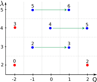
Figure 1: The uncolored Kauffman homology of the trefoil. The label with each dot stands for the homological $t_{r}$-degree and $t_{c}$-degree. The green arrows represent the universal differential $d^{\rm univ}_{\to}$ where the red dots represent the elements in $H_{*}(\widetilde{}\mathscr{H}^{\rm Kauffman}_{[1]}({\bf 3_{1}}),d^{\rm univ}_{\to})$. The red and blue dots correspond to the terms colored with red and blue in (5.1) respectively.

Next, let us investigate the $[2]$-colored Kauffman homology using the properties in §4. In fact, the $[2]$-colored Kauffman polynomial can be simply computed by the Rosso-Jones formula. In addition, it is easy to obtain the $[2]$-colored $\mathfrak{so}(3)$ homology and $\mathfrak{so}(4)$ homology of the trefoil from (191)

$$\mathscr{F}_{\yng(2)}({\bf 3_{1}};q^{2},q,t_{r}=t,t_{c}=1) = \mathscr{P}^{\mathfrak{so}(3)}_{\yng(2)}({\bf 3_{1}};q,t)=\widetilde{}\mathscr{P}_{\yng(4)}({\bf 3_{1}};q,q^{1/2},tq^{-1/2},q^{1/2})~{},$$ (193)

$$\mathscr{F}_{\yng(2)}({\bf 3_{1}};q^{3},q,t_{r}=t,t_{c}=1) = \mathscr{P}^{\mathfrak{so}(4)}_{\yng(2)}({\bf 3_{1}};q,t)=\left[\widetilde{}\mathscr{P}_{\yng(2)}({\bf 3_{1}};q^{2},q,tq^{-1},q)\right]^{2}~{}.$$ (194)

With the canceling differential $d_{[2]\to[0]}$, these data uniquely determine the Poincaré polynomial (546) of the $[2]$-colored triply-graded Kauffman homology in the $t_{r}$-grading. Note that Figure 9 shows how the universal colored differential $d^{\leftarrow}$ acts on the triply-graded homology. Since the trefoil is a thin knot, it is easy to find the $t_{c}$-grading in (546) by using $\delta$-grading (95), where the $S$-invariant $S({\bf 3_{1}})$ of the trefoil is $2$. Then, through (74), one can write the tilde-version of the $[2]$-colored quadruply-graded Kauffman homology with the $(\lambda,Q,t_{r},t_{c})$-gradings (562).

Proceeding further, we will try to obtain the $[r]$-colored Kauffman homology, making use of the refined exponential growth property (102). Actually, the refined exponential growth property is so powerful that it specifies the form of the $[r]$-colored quadruply-graded Kauffman homology at the $t_{c}=1$ specialization

$$\widetilde{}\mathscr{F}_{[r]}({\bf 3_{1}};\lambda,Q,t_{r},t_{c}=1)=\left[\widetilde{}\mathscr{F}_{[1]}({\bf 3_{1}};\lambda,Q,t_{r},t_{c}=1)\right]^{r}$$ (195)

$$= \sum_{k=0}^{r}\left(\begin{array}[]{c}r\\ k\end{array}\right){\color[rgb]{1,0,0}\left[\lambda^{2}Q^{2}t_{r}^{2}(1+Q^{-4}t_{r}^{-2}(1+\lambda^{2}t_{r}^{3}))\right]^{k}}$$ (199)

$$\hskip 142.26378pt\times{\color[rgb]{0,0,1}\left[\lambda^{3}Q^{-1}t_{r}^{2}(1+Q^{2}t_{r})(1+\lambda Qt_{r}^{2}(1+\lambda Q^{-1}t_{r}))\right]^{r-k}}~{},$$

$$= \sum_{k=0}^{r}\sum_{j=0}^{k}\sum_{i=0}^{r-k}\left(\begin{array}[]{c}r\\ k\end{array}\right){\color[rgb]{1,0,0}\lambda^{2k}Q^{2(k-2j)}t_{r}^{2(k-j)}\left(\begin{array}[]{c}k\\ j\end{array}\right)(1+\lambda^{2}t_{r}^{3})^{j}}$$ (207)

$$\hskip 56.9055pt\times{\color[rgb]{0,0,1}\lambda^{3(r-k)+i}Q^{i+k-r}t_{r}^{2(r-k+i)}\left(\begin{array}[]{c}r-k\\ i\end{array}\right)(1+Q^{2}t_{r})^{r-k}(1+\lambda Q^{-1}t_{r})^{i}}~{}.$$

To obtain the full expression, $t_{c}$-gradings remain to be determined. First of all, the binomials in (195) are replaced by the $t_{c}^{2}$-binomials: e.g. $\left(\begin{array}[]{c}r\\ k\end{array}\right)$ in (195) is restored to $\left[\begin{array}[]{c}r\\ k\end{array}\right]_{t_{c}^{2}}$. In addition, the factors with red color at $k=r$ accord to the homology $H_{*}(\widetilde{}\mathscr{H}^{\rm Kauffman}_{[r]}({\bf 3_{1}}),d^{{\rm univ}}_{\to})$ with respect to the universal differential $d^{\rm univ}_{\to}$ and therefore is identical to the form

$$\widetilde{}\mathscr{F}(\widetilde{}\mathscr{H}_{[r]}^{\rm Kauffman}({\bf 3_{1}}),d^{\rm univ}_{\to})(\lambda,Q,t_{r},t_{c})=Q^{2r}\widetilde{}\mathscr{P}_{[r]}({\bf 3_{1}};\lambda Q^{-1},Q,t_{r},t_{c})~{}.$$ (208)

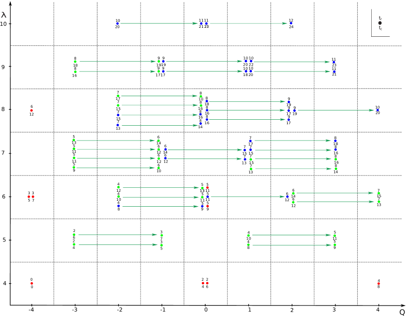
Figure 11: The universal differential $d^{\rm univ}_{\to}$ acts on the $[2]$-colored quadruply-graded Kauffman homology of the trefoil. The red dots represent the elements in $H_{*}(\widetilde{}\mathscr{H}^{\rm Kauffman}_{[2]}({\bf 3_{1}}),d^{\rm univ}_{\to})$. The red, green and blue dots consist of the terms corresponding to $k=2,1$ and $0$ in the first summation of (209) respectively.

Moreover, the form for the red factor is roughly of the form $Q^{2k}\widetilde{}\mathscr{P}_{[k]}({\bf 3_{1}};\lambda Q^{-1},Q,t_{r},t_{c})$ while the $t_{c}$-grading has to be modified in general. On the other hand, the factors colored in blue are killed by the universal differential $d_{\to}^{\rm univ}$. (See Figure 11.) This can be realized by uplifting the term $(1+Q^{2}t_{r})^{r-k}$ in (195) to the $t_{c}^{2}$-Pochhammer symbol $(-Q^{2}t_{r}t_{c};t_{c}^{2})_{r-k}$, which is very natural, judging from the homological elements in the top $\lambda$-degree in Figure 11. In a similar fashion, the $t_{c}^{2}$-Pochhammer symbol $(-\lambda Q^{-1}t_{r}t_{c}^{*};t_{c}^{2})_{i}$ is substituted for the term $(1+\lambda Q^{-1}t_{r})^{i}$ in (195), although the $t_{c}$-degrees in the argument has to be fixed. To incorporate $t_{c}$-gradings appropriately, the explicit expression (552) of the $[2]$-colored quadruply-graded Kauffman homology is inevitable.

By fixing $t_{c}$-gradings in such a way that all the properties in §4 are satisfied, we find the Poincaré polynomial of the $[r]$-colored quadruply-graded Kauffman homology of the trefoil

$$\widetilde{}\mathscr{F}_{[r]}({\bf 3_{1}};\lambda,Q,t_{r},t_{c})$$ (209)

$$= \sum_{k=0}^{r}\sum_{j=0}^{k}\sum_{i=0}^{r-k}\left[\begin{array}[]{c}r\\ k\end{array}\right]_{t_{c}^{2}}{\color[rgb]{1,0,0}\lambda^{2k}Q^{2(k-2j)}t_{r}^{2(k-j)}t_{c}^{2r(k-j)}\left[\begin{array}[]{c}k\\ j\end{array}\right]_{t_{c}^{2}}(-\lambda^{2}t_{r}^{3}t_{c}^{1+2r};t_{c}^{2})_{j}}$$ (217)

$$\times{\color[rgb]{0,0,1}\lambda^{3(r-k)+i}Q^{i+k-r}t_{r}^{2(r-k+i)}t_{c}^{2r(r-k+i)+2ij}\left[\begin{array}[]{c}r-k\\ i\end{array}\right]_{t_{c}^{2}}(-Q^{2}t_{r}t_{c};t_{c}^{2})_{r-k}(-\lambda Q^{-1}t_{r}t_{c};t_{c}^{2})_{i}}$$

$$= \sum_{k=0}^{r}\sum_{j=0}^{k}\sum_{i=0}^{r-k}\lambda^{i-k+3r}Q^{i-4j+3k-r}t_{r}^{2(i-j+r)}t_{c}^{2r(r-j)+2i(j+r)}\left[\begin{array}[]{c}r\\ k\end{array}\right]_{t_{c}^{2}}\left[\begin{array}[]{c}k\\ j\end{array}\right]_{t_{c}^{2}}\left[\begin{array}[]{c}r-k\\ i\end{array}\right]_{t_{c}^{2}}$$ (225)

$$\hskip 85.35826pt\times(-\lambda^{2}t_{r}^{3}t_{c}^{1+2r};t_{c}^{2})_{j}(-Q^{2}t_{r}t_{c};t_{c}^{2})_{r-k}(-\lambda Q^{-1}t_{r}t_{c};t_{c}^{2})_{i}~{}.$$

Apart from the refined exponential growth property and the universal differential, one can check that the formula has the following properties.

• $\mathscr{H}^{\mathfrak{so}(3)}_{[r]}\cong\mathscr{H}^{\mathfrak{sl}(2)}_{[2r]}$ [(134)]

  $$\widetilde{}\mathscr{F}_{[r]}({\bf 3_{1}};q^{2},q,t_{r}q^{-1},q)=\widetilde{}\mathscr{P}_{[2r]}({\bf 3_{1}};q,q^{1/2},t_{r}q^{-1/2},q^{1/2})$$

• $\mathscr{H}^{\mathfrak{so}(4)}_{[r]}\cong\mathscr{H}^{\mathfrak{sl}(2)\oplus\mathfrak{sl}(2)}_{[r]}$ [(137)]

  $$\widetilde{}\mathscr{F}_{[r]}({\bf 3_{1}};q^{3},q,t_{r}q^{-1},t_{c}q)=\left[\widetilde{}\mathscr{P}_{[r]}({\bf 3_{1}};q^{2},q,t_{r}q^{-1},t_{c}q)\right]^{2}$$

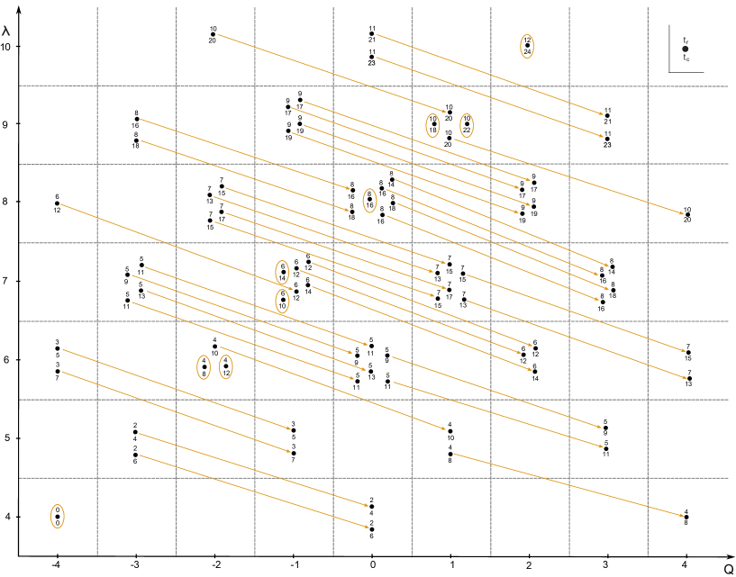
Figure 14: The diagonal differential $d_{\rm diag}^{+}$ acts on the $[2]$-colored quadruply-graded Kauffman homology of the trefoil. The dots enclosed by light brown circles represent the elements in $H_{*}(\widetilde{}\mathscr{H}^{{\rm Kauffman}}_{[2]}({\bf 3_{1}}),d_{\rm diag}^{+})$. It is easy to see that they are aligned along the diagonal line $\lambda(x)-Q(x)=8$. The homology $H_{*}(\widetilde{}\mathscr{H}^{{\rm Kauffman}}_{[2]}({\bf 3_{1}}),d_{\rm diag}^{+})$ is isomorphic to the uncolored homology $\widetilde{}\mathscr{H}^{{\rm HOMFLY}}_{[2]}({\bf 3_{1}})$.

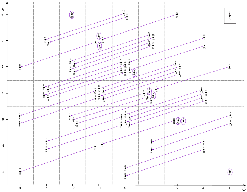
Figure 15: The diagonal differential $d_{\rm diag}^{-}$ acts on the $[2]$-colored quadruply-graded Kauffman homology of the trefoil. The dots enclosed by violet circles represent the elements in $H_{*}(\widetilde{}\mathscr{H}^{{\rm Kauffman}}_{[2]}({\bf 3_{1}}),d_{\rm diag}^{-})$. It is easy to see that they are aligned along the diagonal line $\lambda(x)+Q(x)=8$. The homology $H_{*}(\widetilde{}\mathscr{H}^{{\rm Kauffman}}_{[2]}({\bf 3_{1}}),d_{\rm diag}^{-})$ is isomorphic to the uncolored homology $\widetilde{}\mathscr{H}^{{\rm HOMFLY}}_{[2]}({\bf 3_{1}})$.

• Diagonal differentials $d^{\pm}_{\rm diag}$ [(150), Figure 14 and Figure 15]
  

  $$\widetilde{}\mathscr{F}(\widetilde{}\mathscr{H}^{{\rm Kauffman}}_{[r]}({\bf 3_{1}}),d^{+}_{\rm diag})(\lambda,Q,t_{r},t_{c}) = \tfrac{\lambda^{r}}{Q^{3r}t_{r}^{r}t_{c}^{r}}\widetilde{}\mathscr{P}_{[r]}({\bf 3_{1}};\lambda Qt_{r}t_{c},(\lambda Qt_{r}t_{c})^{\frac{1}{2}},t_{r}t_{c}^{-1},t_{c}^{2})$$

  $$\widetilde{}\mathscr{F}(\widetilde{}\mathscr{H}^{{\rm Kauffman}}_{[r]}({\bf 3_{1}}),d^{-}_{\rm diag})(\lambda,Q,t_{r},t_{c}) = \lambda^{r}Q^{3r}t_{r}^{2r}t_{c}^{2r^{2}}\widetilde{}\mathscr{P}_{[r]}({\bf 3_{1}};\lambda Q^{-1},(\lambda Q^{-1})^{\frac{1}{2}},t_{r},t_{c})$$

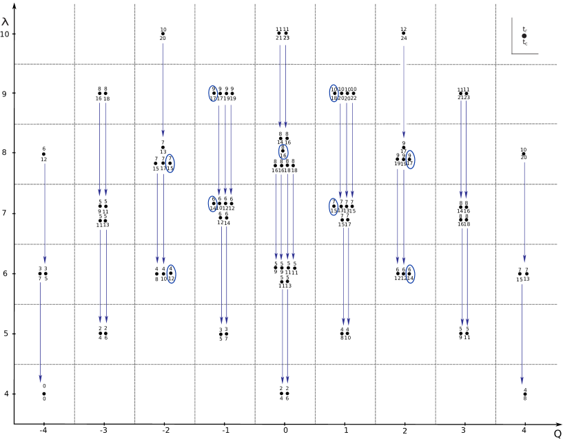
Figure 12: The colored differential $d_{[2]\to[1]}^{-}$ acts on the $[2]$-colored quadruply-graded Kauffman homology of the trefoil. The dots enclosed by blue circles represent the elements in $H_{*}(\widetilde{}\mathscr{H}^{{\rm Kauffman}}_{[2]}({\bf 3_{1}}),d_{[2]\to[1]}^{-})$. One can convince oneself that the homology $H_{*}(\widetilde{}\mathscr{H}^{{\rm Kauffman}}_{[2]}({\bf 3_{1}}),d_{[2]\to[1]}^{-})$ is isomorphic to the uncolored homology $\widetilde{}\mathscr{H}^{{\rm Kauffman}}_{[1]}({\bf 3_{1}})$ shown in Figure 1.

• Colored differential $d^{-}_{[r]\to[\ell]}$ [(176) and Figure 12]
  

  $$\widetilde{}\mathscr{F}(\widetilde{}\mathscr{H}^{\rm Kauffman}_{[r]}({\bf 3_{1}}),d^{-}_{[r]\to[\ell]})(\lambda,Q,t_{r},t_{c})=(\lambda t_{r})^{4(r-\ell)}t_{c}^{4(r^{2}-\ell^{2})}\widetilde{}\mathscr{F}_{[\ell]}({\bf 3_{1}};\lambda,Q,t_{r},t_{c})$$

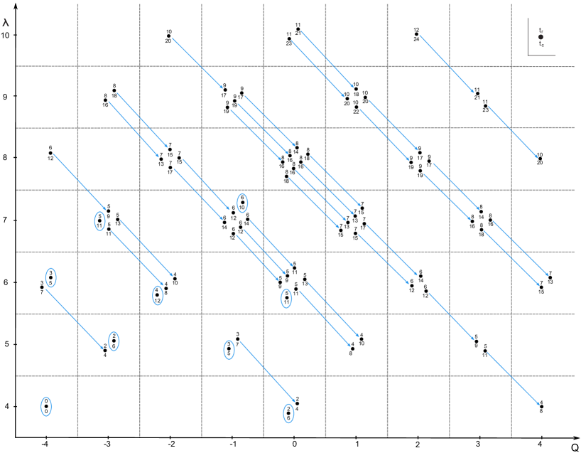
Figure 13: The colored differential $d_{[2]\to[1]}^{+}$ acts on the $[2]$-colored quadruply-graded Kauffman homology of the trefoil. The dots enclosed by light blue circles represent the elements in $H_{*}(\widetilde{}\mathscr{H}^{{\rm Kauffman}}_{[2]}({\bf 3_{1}}),d_{[2]\to[1]}^{-})$. One can convince oneself that the homology $H_{*}(\widetilde{}\mathscr{H}^{{\rm Kauffman}}_{[2]}({\bf 3_{1}}),d_{[2]\to[1]}^{+})$ is isomorphic to the uncolored homology $\widetilde{}\mathscr{H}^{{\rm Kauffman}}_{[1]}({\bf 3_{1}})$ shown in Figure 1.

• Colored differential $d^{+}_{[r]\to[\ell]}$ [Figure 13]
  The Poincaré polynomial of the homology with respect to the colored differential $d^{+}_{[r]\to[\ell]}$ is given by

  $$\widetilde{}\mathscr{F}(\widetilde{}\mathscr{H}^{\rm Kauffman}_{[r]}({\bf 3_{1}}),d_{[r]\to{[\ell]}}^{+})(\lambda,Q,t_{r},t_{c})$$

  $$= \lambda^{2(r-\ell)}Q^{-2(r-\ell)}$$

  $$\times\sum_{k=0}^{\ell}\sum_{j=0}^{k}\sum_{i=0}^{\ell-k}\left[\begin{array}[]{c}\ell\\ k\end{array}\right]_{t_{c}^{2}}{\color[rgb]{1,0,0}\lambda^{2k}Q^{2(k-2j)}t_{r}^{2(k-j)}t_{c}^{2(2r-\ell)(k-j)}\left[\begin{array}[]{c}k\\ j\end{array}\right]_{t_{c}^{2}}(-\lambda^{2}t_{r}^{3}t_{c}^{1+2r};t_{c}^{2})_{j}}$$

  $$\times{\color[rgb]{0,0,1}\lambda^{3(\ell-k)+i}Q^{i+k-\ell}t_{r}^{2(\ell-k+i)}t_{c}^{2(2r-\ell)(\ell-k+i)+2ij}\left[\begin{array}[]{c}\ell-k\\ i\end{array}\right]_{t_{c}^{2}}}$$

  $$\times{\color[rgb]{0,0,1}(-Q^{2}t_{r}t_{c}^{1-2(r-\ell)};t_{c}^{2})_{\ell-k}(-\lambda Q^{-1}t_{r}t_{c}^{1-2(r-\ell)};t_{c}^{2})_{i}}~{}.$$

  Then, one can verify (180):

  $$\widetilde{}\mathscr{F}(\widetilde{}\mathscr{H}^{\rm Kauffman}_{[r]}({\bf 3_{1}}),d^{+}_{[r]\to[\ell]})(q^{3},q,q^{-1}t_{r},qt_{c})=t_{c}^{4(r-\ell)\ell}\left[\widetilde{}\mathscr{P}_{[\ell]}({\bf 3_{1}};q^{2},qt_{c}^{r-\ell},q^{-1}t_{r},qt_{c})\right]^{2}~{}.$$

It is straightforward from (98) to obtain the Poincaré polynomial of the $[r]$-colored triply-graded Kauffman homology of the trefoil in the $t_{r}$-grading

$$\mathscr{F}_{[r]}({\bf 3_{1}};\lambda,q,t_{r}=t,t_{c}=1)=\widetilde{}\mathscr{F}_{[r]}({\bf 3_{1}};\lambda,q,q^{-1}t,q)$$ (228)

$$= \sum_{k=0}^{r}\sum_{j=0}^{k}\sum_{i=0}^{r-k}\lambda^{i-k+3r}q^{3k-2j(1+r)+r(2r-3)+i(2j+2r-1)}t^{2(i-j+r)}\left[\begin{array}[]{c}r\\ k\end{array}\right]_{q^{2}}\left[\begin{array}[]{c}k\\ j\end{array}\right]_{q^{2}}\left[\begin{array}[]{c}r-k\\ i\end{array}\right]_{q^{2}}$$ (236)

$$\hskip 85.35826pt\times(-\lambda^{2}t^{3}q^{2r-2};q^{2})_{j}(-q^{2}t;q^{2})_{r-k}(-\lambda q^{-1}t;q^{2})_{i}~{}.$$

We verify that the expression reduces to colored Kauffman polynomial computed by the Rosso-Jones formula Stevan:2010jh at $t=-1$ up to 4 boxes.

In addition, the mirror/transposition symmetry (100) tells us the Poincaré polynomial of the $[1^{r}]$-colored triply-graded Kauffman homology of the trefoil in the $t_{c}$-grading

$$\mathscr{F}_{[1^{r}]}({\bf 3_{1}};\lambda,q,t_{r},=1,t_{c}=t)=\widetilde{}\mathscr{F}_{[1^{r}]}({\bf 3_{1}};\lambda,q^{r},q^{-1},qt)=\widetilde{}\mathscr{F}_{[r]}({\bf 3_{1}};\lambda,q^{-1}t^{-1},qt,q^{-1})$$ (237)

$$= \sum_{k=0}^{r}\sum_{j=0}^{k}\sum_{i=0}^{r-k}\lambda^{i-k+3r}q^{-3k+2j(1+r)-r(2r-3)-i(2j+2r-1)}t^{i+2j-3k+3r}\left[\begin{array}[]{c}r\\ k\end{array}\right]_{q^{-2}}\left[\begin{array}[]{c}k\\ j\end{array}\right]_{q^{-2}}\left[\begin{array}[]{c}r-k\\ i\end{array}\right]_{q^{-2}}$$ (245)

$$\hskip 85.35826pt\times(-\lambda^{2}t^{3}q^{2-2r};q^{-2})_{j}(-q^{-2}t^{-1};q^{-2})_{r-k}(-\lambda qt^{2};q^{-2})_{i}~{}.$$

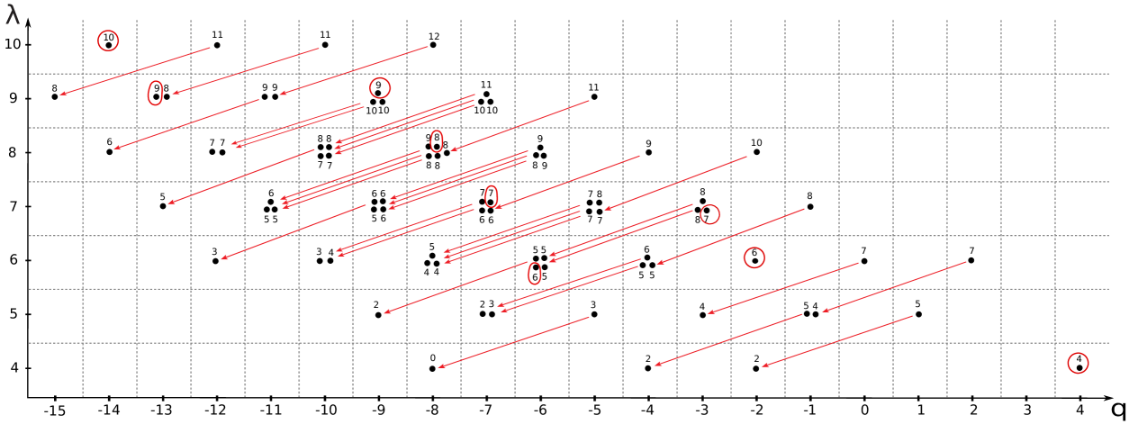
Figure 10: The $[1^{2}]$-colored Kauffman homology of the trefoil. The dots enclosed by red circles represent the elements in $H_{*}(\mathscr{H}^{{\rm Kauffman}}_{[1^{2}]},d_{-2})$.

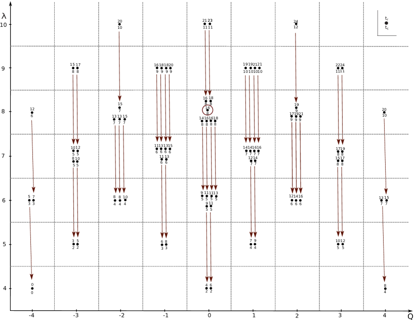
Figure 16: The canceling differential $d_{[1^{r}]\to[0]}^{+}$ acts on the $[1^{2}]$-colored quadruply-graded Kauffman homology of the trefoil.

For instance, the homology diagrams of the $[1^{2}]$-colored Kauffman homology of the trefoil are depicted in Figure 10 for the triple-gradings and Figure 16 for the quadruple-gradings. Especially, in Figure 10, one can see the action of the differential $d_{-2}$, providing the $[2]$-colored $\mathfrak{sp}(2)$ homology of the trefoil

$$\mathscr{P}_{\yng(2)}^{\mathfrak{sp}(2)}({\bf 3_{1}};q,t) = t^{-4}\mathscr{F}(\mathscr{H}^{\rm Kauffman}_{\yng(1,1)}({\bf 3_{1}}),d_{-2})(\lambda=q^{3},q^{-1},1,t)=\widetilde{}\mathscr{P}_{\yng(2)}({\bf 3_{1}};q^{4},q^{2},tq^{-2},q^{2})$$ (246)

$$= q^{8}+q^{20}t^{2}+q^{24}t^{2}+q^{24}t^{3}+q^{28}t^{3}+q^{32}t^{4}+q^{36}t^{5}+q^{40}t^{5}+q^{44}t^{6}~{}.~{}~{}~{}~{}~{}$$ (247)

(See also (551).)

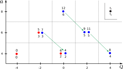
Figure 2: The $[1,1]$-colored HOMFLY homology of the trefoil. The green arrows represent the colored differential $d^{+}_{[1,1]\to[1]}$ where the red dots are the elements in $H_{*}(\widetilde{}\mathscr{H}^{\rm HOMFLY}_{[1,1]}({\bf 3_{1}}),d^{+}_{[1,1]\to[1]})$. The red and blue dots correspond to the factors colored with red and blue in (5.1) respectively.

Having studied the $[r]$-colored Kauffman homology of the trefoil, the next goal is to obtain the $[r,r]$-colored HOMFLY homology of the trefoil using the relation to the $[r]$-colored Kauffman homology predicted in §4. First, it is useful to review the case of $r=1$ Gukov:2011ry . The expression for the $[1,1]$-colored HOMFLY homology follows from (188) via the mirror/transposition symmetry

$$\widetilde{}\mathscr{P}_{\yng(1,1)}({\bf 3_{1}};a,Q,t_{r},t_{c}) = {\color[rgb]{1,0,0}a^{4}\left(Q^{-4}+t_{r}^{6}t_{c}^{2}\right)+a^{6}Q^{-2}t_{r}^{5}t_{c}^{3}}$$

$$+{\color[rgb]{0,0,1}a^{4}\left(t_{r}^{4}t_{c}^{2}+Q^{4}t_{r}^{8}t_{c}^{4}\right)+a^{6}\left(Q^{-2}t_{r}^{7}t_{c}^{3}+Q^{2}(t_{r}^{9}+t_{r}^{11})t_{c}^{5}\right)+a^{8}t_{r}^{12}t_{c}^{6}}~{}.$$

A simple calculation involving (5.1) and (5.1) confirms that

$$\widetilde{}\mathscr{F}_{\yng(1)}({\bf 3_{1}};\lambda=q^{5},q,q^{-1},qt)=\widetilde{}\mathscr{P}_{\yng(1,1)}({\bf 3_{1}};a=q^{4},q,q^{-1},qt)~{}.$$ (249)

In fact, when comparing Figure 2 with Figure 1 in the $t_{c}$-grading, it is easy to see the one-to-one correspondence between the generators of Kauffman homology and those of HOMFLY homology. In addition, the differential $d^{+}_{[1,1]\to[1]}$ in HOMFLY homology clearly corresponds to $d^{{\rm univ}}_{\to}$ in Kauffman homology. Thus, to make an analogy to Kauffman homology, it is convenient to separate the homology $H_{*}(\mathscr{H}^{{\rm HOMFLY}}_{[1,1]},d^{+}_{[1,1]\to[1]})$ with respect to the differential $d^{+}_{[1,1]\to[1]}$ (red color) from the exact elements under the differential $d^{+}_{[1,1]\to[1]}$ (blue color).

Like the colored Kauffman homology (195), with the great help of the refined exponential growth property (84), one can evaluate the $t_{c}=1$ specialization of the $[r,r]$-colored quadruply-graded HOMFLY homology

$$\widetilde{}\mathscr{P}_{[r,r]}({\bf 3_{1}};a,Q,t_{r},t_{c}=1)=\left[\widetilde{}\mathscr{P}_{[1,1]}({\bf 3_{1}};\lambda,Q,t_{r},t_{c}=1)\right]^{r}$$ (250)

$$= \sum_{k=0}^{r}\left(\begin{array}[]{c}r\\ k\end{array}\right){\color[rgb]{1,0,0}\left[a^{4}t_{r}^{6}(1+Q^{-4}t_{r}^{-6}(1+a^{2}Q^{2}t_{r}^{5}))\right]^{k}}$$ (254)

$$\hskip 142.26378pt{\color[rgb]{0,0,1}\left[a^{4}t_{r}^{4}(1+a^{2}Q^{-2}t_{r}^{3})(1+Q^{4}t_{r}^{4}(1+a^{2}Q^{-2}t_{r}))\right]^{r-k}}~{},$$

$$= \sum_{k=0}^{r}\sum_{j=0}^{k}\sum_{i=0}^{r-k}\left(\begin{array}[]{c}r\\ k\end{array}\right){\color[rgb]{1,0,0}a^{4k}Q^{-4j}t_{r}^{6(k-j)}\left(\begin{array}[]{c}k\\ j\end{array}\right)(1+a^{2}Q^{2}t_{r}^{5})^{j}}$$ (262)

$$\hskip 56.9055pt\times{\color[rgb]{0,0,1}a^{4(r-k)}Q^{4i}t_{r}^{4(r-k+i)}\left(\begin{array}[]{c}r-k\\ i\end{array}\right)(1+a^{2}Q^{-2}t_{r}^{3})^{r-k}(1+a^{2}Q^{-2}t_{r})^{i}}~{}.$$

On the other hand, the isomorphism $(\mathfrak{sl}(4),[r,r])\cong(\mathfrak{so}(6),[r])$ can be seen in the identity with the $t_{c}$-grading at the naive specialization $\lambda=q^{5}$ and $a=q^{4}$

$$\widetilde{}\mathscr{F}_{[r]}({\bf 3_{1}};\lambda=q^{5},q,q^{-1},qt_{c})=\widetilde{}\mathscr{P}_{[r,r]}({\bf 3_{1}};a=q^{4},q^{2},q^{-1},qt_{c})~{},$$ (263)

since the trefoil is homologically thin. Thus, this relation helps us determine the $t_{c}$-degrees in (250) by using the formula (209). Consequently, the Poincaré polynomial of the $[r,r]$-colored quadruply-graded HOMFLY homology of the trefoil can be written as

$$\widetilde{}\mathscr{P}_{[r,r]}({\bf 3_{1}};a,Q,t_{r},t_{c})$$ (264)

$$= \sum_{k=0}^{r}\sum_{j=0}^{k}\sum_{i=0}^{r-k}\left[\begin{array}[]{c}r\\ k\end{array}\right]_{t_{c}^{2}}{\color[rgb]{1,0,0}a^{4k}Q^{-4j}t_{r}^{6(k-j)}t_{c}^{2r(k-j)}\left[\begin{array}[]{c}k\\ j\end{array}\right]_{t_{c}^{2}}(-a^{2}Q^{2}t_{r}^{5}t_{c}^{1+2r};t_{c}^{2})_{j}}$$ (272)

$$\times{\color[rgb]{0,0,1}a^{4(r-k)}Q^{4i}t_{r}^{4(r-k+i)}t_{c}^{2i(j+r)+2r(r-k)}\left[\begin{array}[]{c}r-k\\ i\end{array}\right]_{t_{c}^{2}}(-a^{2}Q^{-2}t_{r}^{3}t_{c};t_{c}^{2})_{r-k}(-a^{2}Q^{-2}t_{r}t_{c};t_{c}^{2})_{i}}$$

$$= \sum_{k=0}^{r}\sum_{j=0}^{k}\sum_{i=0}^{r-k}a^{4r}Q^{4(i-j)}t_{r}^{2(2i-3j+k+2r)}t_{c}^{2r(r-j)+2i(j+r)}\left[\begin{array}[]{c}r\\ k\end{array}\right]_{t_{c}^{2}}\left[\begin{array}[]{c}k\\ j\end{array}\right]_{t_{c}^{2}}\left[\begin{array}[]{c}r-k\\ i\end{array}\right]_{t_{c}^{2}}$$ (280)

$$\hskip 85.35826pt\times(-a^{2}Q^{2}t_{r}^{5}t_{c}^{1+2r};t_{c}^{2})_{j}(-a^{2}Q^{-2}t_{r}^{3}t_{c};t_{c}^{2})_{r-k}(-a^{2}Q^{-2}t_{r}t_{c};t_{c}^{2})_{i}~{}.$$

It is easy to confirm that the formula reproduces the $[2,2]$-colored HOMFLY homology of the trefoil obtained in §4.4 of Gorsky:2013jxa . By using (188), one can check that the formula (264) satisfies the other refined exponential growth property (85)

$$\widetilde{}\mathscr{P}_{[r,r]}({\bf 3_{1}};a,Q,1,t_{c})=\left[\widetilde{}\mathscr{P}_{[r]}({\bf 3_{1}};a,Q,1,t_{c})\right]^{2}~{},$$ (281)

with small values of $r$. In addition, the formula shows the behaviors of the colored differentials predicted in Gorsky:2013jxa :

$$\widetilde{}\mathscr{P}(\mathscr{H}^{\rm HOMFLY}_{[r,r]}({\bf 3_{1}}),d^{+}_{[r,r]\to[\ell,\ell]})(a,Q,t_{r},t_{c}) = [aQ^{-1}t_{c}^{\ell}]^{4(r-\ell)}\widetilde{}\mathscr{P}_{[\ell,\ell]}({\bf 3_{1}};a,Qt_{c}^{r-\ell},t_{r},t_{c})~{},$$ (282)

$$\widetilde{}\mathscr{P}(\mathscr{H}^{\rm HOMFLY}_{[r,r]}({\bf 3_{1}}),d^{-}_{[r,r]\to[\ell,\ell]})(a,Q,t_{r},t_{c}) = [aQt_{r}^{2}t_{c}^{(r+\ell)}]^{4(r-\ell)}\widetilde{}\mathscr{P}_{[\ell,\ell]}({\bf 3_{1}};a,Q,t_{r},t_{c})~{},$$ (283)

$$\widetilde{}\mathscr{P}(\mathscr{H}^{\rm HOMFLY}_{[r,r]}({\bf 3_{1}}),d^{+}_{[r,r]\to[r]})(a,Q,t_{r},t_{c}) = a^{2r}Q^{-2r}t_{r}^{2r}\widetilde{}\mathscr{P}_{[r]}({\bf 3_{1}};a,Qt_{r},t_{r},t_{c})~{},$$ (284)

$$\widetilde{}\mathscr{P}(\mathscr{H}^{\rm HOMFLY}_{[r,r]}({\bf 3_{1}}),d^{-}_{[r,r]\to[r]})(a,Q,t_{r},t_{c}) = a^{2r}Q^{2r}t_{r}^{6r}t_{c}^{2r^{2}}\widetilde{}\mathscr{P}_{[r]}({\bf 3_{1}};a,Q,t_{r},t_{c})~{}.$$ (285)

This is actually expected since the colored differentials in the $[r,r]$-colored HOMFLY homology have their own counterparts in the $[r]$-colored Kauffman homology as we see in §4, and we have seen that the formula (209) analogous to (264) is endowed with the correct differential structure. Furthermore, we have verified that the Poincaré polynomials with the $t_{c}$-grading $\widetilde{}\mathscr{P}_{[r,r]}({\bf 3_{1}};a,q,q^{-1},qt)$ agree with the corresponding refined Chern-Simons invariants computed in Shakirov:2013moa up to $r=3$.

As in the Kauffman homology, the Poincaré polynomial of the $[r,r]$-colored triply-graded HOMFLY homology of the trefoil in the $t_{r}$-grading immediately follows:

$$\mathscr{P}_{[r,r]}({\bf 3_{1}};a,q,t_{r}=t,t_{c}=1)=\widetilde{}\mathscr{P}_{[r,r]}({\bf 3_{1}};a,q^{2},q^{-1}t,q)$$ (286)

$$= \sum_{k=0}^{r}\sum_{j=0}^{k}\sum_{i=0}^{r-k}a^{4r}q^{-2(j+k+(2+j)r-r^{2}-i(2+j+r))}t^{2(2i-3j+k+2r)}\left[\begin{array}[]{c}r\\ k\end{array}\right]_{q^{2}}\left[\begin{array}[]{c}k\\ j\end{array}\right]_{q^{2}}\left[\begin{array}[]{c}r-k\\ i\end{array}\right]_{q^{2}}$$ (294)

$$\hskip 85.35826pt\times(-a^{2}q^{2r}t^{5};q^{2})_{j}(-a^{2}q^{-6}t^{3};q^{2})_{r-k}(-a^{2}q^{-4}t;q^{2})_{i}~{}.$$

The mirror/transposition symmetry yields the Poincaré polynomial of the $[2^{r}]$-colored triply-graded HOMFLY homology of the trefoil in the $t_{c}$-grading

$$\mathscr{P}_{[2^{r}]}({\bf 3_{1}};a,q,t_{r}=1,t_{c}=t)=\widetilde{}\mathscr{P}_{[2^{r}]}({\bf 3_{1}};a,q^{r},q^{-1},qt)=\widetilde{}\mathscr{P}_{[r,r]}({\bf 3_{1}};a,q^{r},qt,q^{-1})$$ (295)

$$= \sum_{k=0}^{r}\sum_{j=0}^{k}\sum_{i=0}^{r-k}a^{4r}q^{-2(-k+i(-2+j-r)-2r+r^{2}+j(3+r))}t^{2(2i-3j+k+2r)}\left[\begin{array}[]{c}r\\ k\end{array}\right]_{q^{-2}}\left[\begin{array}[]{c}k\\ j\end{array}\right]_{q^{-2}}\left[\begin{array}[]{c}r-k\\ i\end{array}\right]_{q^{-2}}$$ (303)

$$\hskip 85.35826pt\times(-a^{2}q^{4}t^{5};q^{-2})_{j}(-a^{2}q^{2-2r}t^{3};q^{-2})_{r-k}(-a^{2}q^{-2r}t;q^{-2})_{i}~{}.$$

Setting $r=3$, the formula reproduces the $[2,2,2]$-colored HOMFLY homology of the trefoil in §4.5 of Gorsky:2013jxa .

5.2 Figure-eight

In this subsection, we obtain the $[r]$-colored Kauffman homology and the $[r,r]$-colored HOMFLY homology of the figure-eight. The strategy is the same as the case of the trefoil although the size of the homology is bigger and therefore the computations are more tedious. Hence, we will not repeat the detailed explanations for the method.

As in the case of the trefoil, let us start with writing the Poincaré polynomial of the $[r]$-colored quadruply-graded HOMFLY homology of the figure-eight

$$\widetilde{}\mathscr{P}_{[r]}({\bf 4_{1}};a,Q,t_{r},t_{c}) = \sum_{k=0}^{r}a^{-2k}t_{r}^{-2k}t_{c}^{-2rk}\left[\begin{array}[]{c}r\\ k\end{array}\right]_{t_{c}^{2}}(-a^{2}Q^{-2}t_{r}t_{c};t_{c}^{2})_{k}(-a^{2}Q^{2}t_{r}^{3}t_{c}^{1+2r};t_{c}^{2})_{k}~{}.\quad$$ (306)

The expression $\widetilde{}\mathscr{P}_{[r]}({\bf 4_{1}};a,q,tq^{-1},q)$ for the triply-graded homology in the $t_{r}$-grading is equal to (3.3) in Fuji:2012pi . The uncolored HOMFLY homology of the figure-eight is given in Gukov:2005qp

$$\widetilde{}\mathscr{F}_{\yng(1)}({\bf 4_{1}};\lambda,Q,t_{r},t_{c})$$ (307)

$$= {\color[rgb]{1,0,0}Q^{2}t_{r}^{-2}t_{c}^{-2}{\lambda^{-2}}+Q^{-2}t_{r}^{-1}t_{c}^{-1}+1+Q^{2}t_{r}t_{c}+Q^{-2}t_{r}^{2}t_{c}^{2}\lambda^{2}}$$

$$+{\color[rgb]{0,0,1}\left(Q^{-2}t_{r}^{-4}t_{c}^{-4}+t_{r}^{-3}t_{c}^{-3}\right){\lambda^{-2}}+\left(Q^{-3}t_{r}^{-3}t_{c}^{-3}+2Q^{-1}t_{r}^{-2}t_{c}^{-2}+2Qt_{r}^{-1}t_{c}^{-1}+Q^{3}\right){\lambda^{-1}}}$$

$${\color[rgb]{0,0,1}+2+Q^{-2}t_{r}^{-1}t_{c}^{-1}+Q^{2}t_{r}t_{c}+\left(Q^{-3}+2Q^{-1}t_{r}t_{c}+2Qt_{r}^{2}t_{c}^{2}+Q^{3}t_{r}^{3}t_{c}^{3}\right)\lambda+\left(t_{r}^{3}t_{c}^{3}+Q^{2}t_{r}^{4}t_{c}^{4}\right)\lambda^{2}}~{},$$

whose homology diagram is presented in Figure 3.

Unlike the case of the trefoil, the colored Kauffman polynomials of the figure-eight are not available to date. However, using the refined exponential growth property, the representation theoretic relation and the differential property, one can uniquely determine the $[2]$-colored Kauffman homology of the figure-eight

$$\mathscr{F}_{\yng(2)}({\bf 4_{1}};\lambda,q,t_{r}=t,t_{c}=1)$$ (310)

$$= \lambda^{-4}\left(\tfrac{1}{q^{12}t^{8}}+\tfrac{1}{q^{10}t^{7}}+\tfrac{1}{q^{8}t^{7}}+\tfrac{2}{q^{6}t^{6}}+\tfrac{1}{q^{4}t^{6}}+\tfrac{1}{q^{4}t^{5}}+\tfrac{1}{q^{2}t^{5}}+\tfrac{1}{t^{4}}\right)$$ (326)

$$+\lambda^{-3}\Big{(}\tfrac{1}{q^{13}t^{7}}+\tfrac{1}{q^{11}t^{7}}+\tfrac{1}{q^{11}t^{6}}+\tfrac{3}{q^{9}t^{6}}+\tfrac{2}{q^{7}t^{6}}+\tfrac{4}{q^{7}t^{5}}+\tfrac{5}{q^{5}t^{5}}+\tfrac{1}{q^{3}t^{5}}+\tfrac{2}{q^{5}t^{4}}+\tfrac{5}{q^{3}t^{4}}+\tfrac{3}{qt^{4}}+\tfrac{3}{qt^{3}}$$

$$\hskip 56.9055pt+\tfrac{3q}{t^{3}}+\tfrac{q}{t^{2}}+\tfrac{q^{3}}{t^{2}}\Big{)}$$

$$+\lambda^{-2}\Big{(}q^{6}+\tfrac{1}{q^{12}t^{6}}+\tfrac{3}{q^{10}t^{5}}+\tfrac{4}{q^{8}t^{5}}+\tfrac{1}{q^{6}t^{5}}+\tfrac{3}{q^{8}t^{4}}+\tfrac{9}{q^{6}t^{4}}+\tfrac{5}{q^{4}t^{4}}+\tfrac{1}{q^{2}t^{4}}+\tfrac{3}{t^{3}}+\tfrac{1}{q^{6}t^{3}}+\tfrac{9}{q^{4}t^{3}}$$

$$\hskip 56.9055pt+\tfrac{11}{q^{2}t^{3}}+\tfrac{10}{t^{2}}+\tfrac{4}{q^{2}t^{2}}+\tfrac{4q^{2}}{t^{2}}+\tfrac{1}{t}+\tfrac{4q^{2}}{t}+\tfrac{3q^{4}}{t}\Big{)}$$

$$+\lambda^{-1}\Big{(}6q+10q^{3}+4q^{5}+\tfrac{1}{q^{11}t^{4}}+\tfrac{3}{q^{9}t^{4}}+\tfrac{2}{q^{7}t^{4}}+\tfrac{1}{q^{9}t^{3}}+\tfrac{7}{q^{7}t^{3}}+\tfrac{9}{q^{5}t^{3}}+\tfrac{3}{q^{3}t^{3}}+\tfrac{7}{q^{5}t^{2}}$$

$$\hskip 56.9055pt+\tfrac{16}{q^{3}t^{2}}+\tfrac{10}{qt^{2}}+\tfrac{q}{t^{2}}+\tfrac{3}{q^{3}t}+\tfrac{14}{qt}+\tfrac{14q}{t}+\tfrac{3q^{3}}{t}+q^{3}t+3q^{5}t+2q^{7}t\Big{)}$$

$$+21+\tfrac{1}{q^{4}}+\tfrac{10}{q^{2}}+10q^{2}+q^{4}+\tfrac{1}{q^{10}t^{3}}+\tfrac{1}{q^{8}t^{3}}+\tfrac{2}{q^{8}t^{2}}+\tfrac{7}{q^{6}t^{2}}+\tfrac{4}{q^{4}t^{2}}+\tfrac{1}{q^{2}t^{2}}+\tfrac{4}{t}+\tfrac{2}{q^{6}t}+\tfrac{12}{q^{4}t}+\tfrac{14}{q^{2}t}$$

$$\hskip 56.9055pt+4t+14q^{2}t+12q^{4}t+2q^{6}t+q^{2}t^{2}+4q^{4}t^{2}+7q^{6}t^{2}+2q^{8}t^{2}+q^{8}t^{3}+q^{10}t^{3}$$

$$+\lambda\Big{(}\tfrac{4}{q^{5}}+\tfrac{10}{q^{3}}+\tfrac{6}{q}+\tfrac{2}{q^{7}t}+\tfrac{3}{q^{5}t}+\tfrac{1}{q^{3}t}+\tfrac{3t}{q^{3}}+\tfrac{14t}{q}+14qt+3q^{3}t+\tfrac{t^{2}}{q}+10qt^{2}$$

$$\hskip 56.9055pt+16q^{3}t^{2}+7q^{5}t^{2}+3q^{3}t^{3}+9q^{5}t^{3}+7q^{7}t^{3}+q^{9}t^{3}+2q^{7}t^{4}+3q^{9}t^{4}+q^{11}t^{4}\Big{)}$$

$$+\lambda^{2}\Big{(}\tfrac{1}{q^{6}}+t+\tfrac{3t}{q^{4}}+\tfrac{4t}{q^{2}}+10t^{2}+\tfrac{4t^{2}}{q^{2}}+4q^{2}t^{2}+3t^{3}+11q^{2}t^{3}+9q^{4}t^{3}+q^{6}t^{3}$$

$$\hskip 56.9055pt+q^{2}t^{4}+5q^{4}t^{4}+9q^{6}t^{4}+3q^{8}t^{4}+q^{6}t^{5}+4q^{8}t^{5}+3q^{10}t^{5}+q^{12}t^{6}\Big{)}$$

$$+\lambda^{3}\Big{(}\tfrac{t^{2}}{q^{3}}+\tfrac{t^{2}}{q}+\tfrac{3t^{3}}{q}+3qt^{3}+3qt^{4}+5q^{3}t^{4}+2q^{5}t^{4}+q^{3}t^{5}+5q^{5}t^{5}+4q^{7}t^{5}+2q^{7}t^{6}+3q^{9}t^{6}$$

$$\hskip 56.9055pt+q^{11}t^{6}+q^{11}t^{7}+q^{13}t^{7}\Big{)}$$

$$+\lambda^{4}\left(t^{4}+q^{2}t^{5}+q^{4}t^{5}+q^{4}t^{6}+2q^{6}t^{6}+q^{8}t^{7}+q^{10}t^{7}+q^{12}t^{8}\right)$$

Here, the expression is written in the triple-grading with the $t_{r}$-grading, and it has 625 generators. Using the $\delta$-grading (95) where the $S$-invariant $S({\bf 4_{1}})$ of the figure-eight is $0$, one can assign the $t_{c}$-gradings in (310). Note that the colored Kauffman homology obeys the following identity since the figure-eight is the same as its mirror image:

$$\mathscr{F}_{[r]}({\bf 4_{1}};\lambda,q,t_{r},t_{c})=\mathscr{F}_{[r]}({\bf 4_{1}};\lambda^{-1},q^{-1},t_{r}^{-1},t_{c}^{-1})~{}.$$ (327)

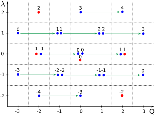
Figure 3: The uncolored Kauffman homology of the figure-eight. The green arrows represent the universal differential $d^{\rm univ}_{\to}$ and the red dots are the elements in $H_{*}(\widetilde{}\mathscr{H}^{\rm Kauffman}_{[1]}({\bf 4_{1}}),d^{\rm univ}_{\to})$. The red and blue dots correspond to the factors colored by red and blue in (307) respectively.

The method to obtain the $[r]$-colored Kauffman homology of the figure-eight is the same as in the case of the trefoil although it is more tedious due to its size. The refined exponential growth property determines the $t_{c}=1$ specialization of the Poincaré polynomial of the $[r]$-colored quadruply-graded Kauffman homology of the figure-eight. Then, the $t_{c}$-gradings are fixed by the differential structure and the $[2]$-colored Kauffman homology, yielding the full expression

$$\widetilde{}\mathscr{F}_{[r]}({\bf 4_{1}};\lambda,Q,t_{r},t_{c})$$ (328)

$$= \sum_{k=0}^{r}\sum_{j=0}^{k}\sum_{i=0}^{r-k}\left[\begin{array}[]{c}r\\ k\end{array}\right]_{t_{c}^{2}}{\color[rgb]{1,0,0}\lambda^{-2j}Q^{2j}t_{r}^{-2j}t_{c}^{-2rj}\left[\begin{array}[]{c}k\\ j\end{array}\right]_{t_{c}^{2}}(-\lambda^{2}Q^{-4}t_{r}t_{c}^{2\left(r-k-i\right)+1};t_{c}^{2})_{j}(-\lambda^{2}t_{r}^{3}t_{c}^{1+4r-2k};t_{c}^{2})_{j}}$$ (337)

$$\times{\color[rgb]{0,0,1}\lambda^{i+2k-2r}Q^{i+2k-2r}t_{r}^{2(i+2k-2r)}t_{c}^{2i(j-k+r)+2(k-r)(j-k+2r)}\left[\begin{array}[]{c}r-k\\ i\end{array}\right]_{t_{c}^{2}}}$$

$$\times{\color[rgb]{0,0,1}(-Q^{2}t_{r}t_{c};t_{c}^{2})_{r-k}(-\lambda^{2}t_{r}^{3}t_{c}^{1+2r};t_{c}^{2})_{r-k}(-\lambda Q^{-1}t_{r}t_{c};t_{c}^{2})_{r-k-i}(-\lambda Q^{3}t_{r}^{3}t_{c}^{1+2(r-k+j)};t_{c}^{2})_{r-k-i}}$$

$$= \sum_{k=0}^{r}\sum_{j=0}^{k}\sum_{i=0}^{r-k}\lambda^{2(k-r-j)+i}Q^{2(k+j-r)+i}t_{r}^{2(2k+i-j-2r)}t_{c}^{-2(k+i-2r)(k-j-r)}\left[\begin{array}[]{c}r\\ k\end{array}\right]_{t_{c}^{2}}\left[\begin{array}[]{c}r-k\\ i\end{array}\right]_{t_{c}^{2}}\left[\begin{array}[]{c}k\\ j\end{array}\right]_{t_{c}^{2}}$$ (346)

$$\times(-\lambda^{2}Q^{-4}t_{r}t_{c}^{2\left(r-k-i\right)+1};t_{c}^{2})_{j}(-\lambda^{2}t_{r}^{3}t_{c}^{1+4r-2k};t_{c}^{2})_{j}(-Q^{2}t_{r}t_{c};t_{c}^{2})_{r-k}(-\lambda^{2}t_{r}^{3}t_{c}^{1+2r};t_{c}^{2})_{r-k}$$

$$\times(-\lambda Q^{-1}t_{r}t_{c};t_{c}^{2})_{r-k-i}(-\lambda Q^{3}t_{r}^{3}t_{c}^{1+2(r-k+j)};t_{c}^{2})_{r-k-i}~{}.$$

By construction, the red factors in (209) are very close to $Q^{2k}\widetilde{}\mathscr{P}_{[k]}({\bf 4_{1}};\lambda Q^{-1},Q,t_{r},t_{c})$ and the blue factors are killed by the universal differential $d^{\rm univ}_{\to}$ due to the presence of the $t_{c}^{2}$-Pochhammer $(-Q^{2}t_{r}t_{c};t_{c}^{2})_{r-k}$. One can check that the formula satisfies all the structural properties innate in the $[r]$-colored Kauffman homology. Subsequently, the Poincaré polynomial of the $[r]$-colored triply-graded Kauffman homology of the figure-eight in the $t_{r}$-grading can be expressed by

$$\mathscr{F}_{[r]}({\bf 4_{1}};\lambda,q,t_{r}=t,t_{c}=1)=\widetilde{}\mathscr{F}_{[r]}({\bf 4_{1}};\lambda,q,q^{-1}t,q)$$ (347)

$$= \sum_{k=0}^{r}\sum_{j=0}^{k}\sum_{i=0}^{r-k}\lambda^{2(k-r-j)+i}q^{4j-2k^{2}-2k(1+i-j-3r)+(i-2r)(2r+2j-1)}t^{2(2k-2r+i-j)}$$ (356)

$$\times\left[\begin{array}[]{c}r\\ k\end{array}\right]_{q^{2}}\left[\begin{array}[]{c}r-k\\ i\end{array}\right]_{q^{2}}\left[\begin{array}[]{c}k\\ j\end{array}\right]_{q^{2}}(-\lambda^{2}q^{2(r-k-i)-4}t;q^{2})_{j}(-\lambda^{2}q^{-2+4r-2k}t^{3};q^{2})_{j}(-q^{2}t;q^{2})_{r-k}$$

$$\times(-\lambda^{2}q^{-2+2r}t^{3};q^{2})_{r-k}(-\lambda q^{-1}t;q^{2})_{r-k-i}(-\lambda q^{1+2(r-k+j)}t^{3};q^{2})_{r-k-i}~{}.$$

The mirror/transposition symmetry provides the Poincaré polynomial of the $[1^{r}]$-colored triply-graded Kauffman homology of the trefoil in the $t_{c}$-grading

$$\mathscr{F}_{[1^{r}]}({\bf 4_{1}};\lambda,q,t_{r}=1,t_{c}=t)=\widetilde{}\mathscr{F}_{[1^{r}]}({\bf 4_{1}};\lambda,q^{r},q^{-1},qt)=\widetilde{}\mathscr{F}_{[r]}({\bf 4_{1}};\lambda,q^{-1}t^{-1},qt,q^{-1})$$ (357)

$$= \sum_{k=0}^{r}\sum_{j=0}^{k}\sum_{i=0}^{r-k}\lambda^{2(k-r-j)+i}q^{-4j+2k^{2}+2k(1+i-j-3r)-(i-2r)(2r+2j-1)}t^{i+2k-2(2j+r)}$$

$$\times\left[\begin{array}[]{c}r\\ k\end{array}\right]_{q^{-2}}\left[\begin{array}[]{c}r-k\\ i\end{array}\right]_{q^{-2}}\left[\begin{array}[]{c}k\\ j\end{array}\right]_{q^{-2}}(-\lambda^{2}q^{-2(r-k-i)+4}t^{5};q^{-2})_{j}(-\lambda^{2}q^{2-4r+2k}t^{3};q^{-2})_{j}$$

$$\times(-q^{-2}t^{-1};q^{-2})_{r-k}(-\lambda^{2}q^{2-2r}t^{3};q^{-2})_{r-k}(-\lambda qt^{2};q^{-2})_{r-k-i}(-\lambda q^{-1-2(r-k+j)};q^{-2})_{r-k-i}~{}.$$

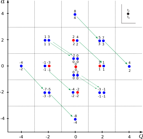
Figure 4: The $[1,1]$-colored HOMFLY homology of the figure-eight. The green arrows represent the colored differential $d^{+}_{[1,1]\to[1]}$ where the red dots are the elements in $H_{*}(\widetilde{}\mathscr{H}^{\rm HOMFLY}_{[1,1]}({\bf 4_{1}}),d^{+}_{[1,1]\to[1]})$. The red and blue dots correspond to the factors colored in red and blue in (370) respectively.

Let us now try to obtain the $[r,r]$-colored HOMFLY homology of the figure-eight. The Poincaré polynomial of the $[1,1]$-colored HOMFLY homology (Figure 4) which can be obtained from (306) by the mirror/transposition symmetry

$$\widetilde{}\mathscr{P}_{\yng(1,1)}({\bf 4_{1}};a,Q,t_{r},t_{c}) = {\color[rgb]{1,0,0}\tfrac{1}{a^{2}t_{c}^{2}t_{r}^{2}}+\tfrac{1}{Q^{2}t_{c}t_{r}^{3}}+1+Q^{2}t_{c}t_{r}^{3}+a^{2}t_{c}^{2}t_{r}^{2}}$$ (369)

$${\color[rgb]{0,0,1}\tfrac{1}{a^{4}t_{c}^{4}t_{r}^{8}}+\tfrac{1}{a^{2}}\left(\tfrac{1}{Q^{2}t_{c}^{3}t_{r}^{7}}+\tfrac{1}{Q^{2}t_{c}^{3}t_{r}^{5}}+\tfrac{1}{t_{c}^{2}t_{r}^{4}}+\tfrac{Q^{2}}{t_{c}t_{r}^{3}}+\tfrac{1}{t_{c}^{2}t_{r}^{2}}+\tfrac{Q^{2}}{t_{c}t_{r}}\right)}$$

$${\color[rgb]{0,0,1}+\tfrac{1}{Q^{4}t_{c}^{2}t_{r}^{4}}+\tfrac{1}{Q^{2}t_{c}t_{r}}+2+\tfrac{1}{t_{r}^{2}}+t_{r}^{2}+Q^{2}t_{c}t_{r}+Q^{4}t_{c}^{2}t_{r}^{4}}$$

$${\color[rgb]{0,0,1}+a^{2}\left(\tfrac{t_{c}t_{r}}{Q^{2}}+\tfrac{t_{c}t_{r}^{3}}{Q^{2}}+t_{c}^{2}t_{r}^{4}+Q^{2}t_{c}^{3}t_{r}^{5}+Q^{2}t_{c}^{3}t_{r}^{7}\right)+a^{4}t_{c}^{4}t_{r}^{8}}~{}.$$

The $t_{c}=1$ specialization of the Poincaré polynomial of the $[r,r]$-colored quadruply-graded HOMFLY homology of the figure-eight is determined by the refined exponential growth property and the $t_{c}$-gradings can be eventually given by using (328). As a result, we can write a closed form expression

$$\widetilde{}\mathscr{P}_{[r,r]}({\bf 4_{1}};a,Q,t_{r},t_{c})$$ (370)

$$= \sum_{k=0}^{r}\sum_{j=0}^{k}\sum_{i=0}^{r-k}\left[\begin{array}[]{c}r\\ k\end{array}\right]_{t_{c}^{2}}{\color[rgb]{1,0,0}a^{-2j}t_{r}^{-2j}t_{c}^{-2rj}\left[\begin{array}[]{c}k\\ j\end{array}\right]_{t_{c}^{2}}(-a^{2}Q^{-2}t_{r}^{-1}t_{c}^{2\left(r-k-i\right)+1};t_{c}^{2})_{j}(-a^{2}Q^{2}t_{r}^{5}t_{c}^{1+4r-2k};t_{c}^{2})_{j}}$$ (379)

$$\times{\color[rgb]{0,0,1}a^{2(i+2k-2r)}t_{r}^{4(i+2k-2r)}t_{c}^{2i(j-k+r)+2(k-r)(j-k+2r)}\left[\begin{array}[]{c}r-k\\ i\end{array}\right]_{t_{c}^{2}}(-a^{2}Q^{-2}t_{r}^{3}t_{c};t_{c}^{2})_{r-k}}$$

$$\times{\color[rgb]{0,0,1}(-a^{2}Q^{2}t_{r}^{5}t_{c}^{1+2r};t_{c}^{2})_{r-k}(-a^{2}Q^{-2}t_{r}t_{c};t_{c}^{2})_{r-k-i}(-a^{2}Q^{2}t_{r}^{7}t_{c}^{1+2(r-k+j)};t_{c}^{2})_{r-k-i}}$$

$$= \sum_{k=0}^{r}\sum_{j=0}^{k}\sum_{i=0}^{r-k}a^{2(i-j+2k-2r)}t_{c}^{2(i+k-2r)(j-k+r)}t_{r}^{4i-2j+8k-8r}\left[\begin{array}[]{c}r\\ k\end{array}\right]_{t_{c}^{2}}\left[\begin{array}[]{c}r-k\\ i\end{array}\right]_{t_{c}^{2}}\left[\begin{array}[]{c}k\\ j\end{array}\right]_{t_{c}^{2}}$$ (388)

$$\times(-a^{2}Q^{-2}t_{r}^{-1}t_{c}^{2\left(r-k-i\right)+1};t_{c}^{2})_{j}(-a^{2}Q^{2}t_{r}^{5}t_{c}^{1+4r-2k};t_{c}^{2})_{j}(-a^{2}Q^{-2}t_{r}^{3}t_{c};t_{c}^{2})_{r-k}$$

$$\times(-a^{2}Q^{2}t_{r}^{5}t_{c}^{1+2r};t_{c}^{2})_{r-k}(-a^{2}Q^{-2}t_{r}t_{c};t_{c}^{2})_{r-k-i}(-a^{2}Q^{2}t_{r}^{7}t_{c}^{1+2(r-k+j)};t_{c}^{2})_{r-k-i}~{}.$$

The Poincaré polynomial of the $[r,r]$-colored triply-graded HOMFLY homology of the figure-eight in the $t_{r}$-grading

$$\mathscr{P}_{[r,r]}({\bf 4_{1}};a,q,t_{r}=t,t_{c}=1)=\widetilde{}\mathscr{P}_{[r,r]}({\bf 4_{1}};a,q^{2},q^{-1}t,q)$$ (389)

$$= \sum_{k=0}^{r}\sum_{j=0}^{k}\sum_{i=0}^{r-k}a^{2(i-j+2k-2r)}q^{2j(1+k-2r)-2(4+k-2r)(k-r)+2i(-2+j-k+r)}t^{4i-2j+8k-8r}$$ (398)

$$\times\left[\begin{array}[]{c}r\\ k\end{array}\right]_{q^{2}}\left[\begin{array}[]{c}r-k\\ i\end{array}\right]_{q^{2}}\left[\begin{array}[]{c}k\\ j\end{array}\right]_{q^{2}}(-a^{2}q^{2\left(r-k-i-1\right)}t^{-1};q^{2})_{j}(-a^{2}q^{4r-2k}t^{5};q^{2})_{j}(-a^{2}q^{-6}t^{3};q^{2})_{r-k}$$

$$\times(-a^{2}q^{2r}t^{5};q^{2})_{r-k}(-a^{2}q^{-4}t;q^{2})_{r-k-i}(-a^{2}q^{2(r-k+j-1)}t^{7};q^{2})_{r-k-i}~{}.$$

Indeed, setting $r=2$, this formula decategorifies at $t=-1$ to the HOMFLY polynomial colored by $[2,2]$-representation written in (E.1) of Anokhina:2013ica . The Poincaré polynomial of the $[2^{r}]$-colored triply-graded HOMFLY homology of the figure-eight in the $t_{c}$-grading can be written as

$$\mathscr{P}_{[2^{r}]}({\bf 4_{1}};a,q,t_{r}=1,t_{c}=t)=\widetilde{}\mathscr{P}_{[2^{r}]}({\bf 4_{1}};a,q^{r},q^{-1},qt)=\widetilde{}\mathscr{P}_{[r,r]}({\bf 4_{1}};a,q^{r},qt,q^{-1})$$ (399)

$$= \sum_{k=0}^{r}\sum_{j=0}^{k}\sum_{i=0}^{r-k}a^{2(i-j+2k-2r)}q^{-2j(1+k-2r)+2(4+k-2r)(k-r)-2i(-2+j-k+r)}t^{4i-2j+8k-8r}$$

$$\times\left[\begin{array}[]{c}r\\ k\end{array}\right]_{q^{-2}}\left[\begin{array}[]{c}r-k\\ i\end{array}\right]_{q^{-2}}\left[\begin{array}[]{c}k\\ j\end{array}\right]_{q^{-2}}(-a^{2}q^{2(-1+i+k-2r)}t^{-1};q^{-2})_{j}(-a^{2}q^{4+2k-2r}t^{5};q^{-2})_{j}$$

$$\times(-a^{2}q^{2-2r}t^{3};q^{-2})_{r-k}(-a^{2}q^{4}t^{5};q^{-2})_{r-k}(-a^{2}q^{-2r}t;q^{-2})_{r-k-i}(-a^{2}q^{6-2j+2k}t^{7};q^{-2})_{r-k-i}~{}.$$

6 Super-$A$-polynomials

In the last fifteen years, remarkable results have been obtained by looking at the large color behaviors of colored Jones polynomials, i.e. the volume conjectures. (See a comprehensive review Murakami:2008 and references therein.) It is apparent that the volume conjecture Kashaev:1996kc ; Murakami:1999 is a key to understanding the relationship between quantum invariants of a knot $K$ and classical geometry of the knot complement $S^{3}\backslash K$. Surprisingly, the large color behavior of colored Jones polynomials is dominated by $SL(2,\mathbb{C})$ flat connections rather than $SU(2)$ Gukov:2003na . Hence, it is more directly related to analytically continued $SL(2,\mathbb{C})$ Chern-Simons theory Gukov:2003na ; Gukov:2006ze ; Witten:2010cx . Let us briefly review the conjecture below.

Let $\mathfrak{g}$ be either $\mathfrak{sl}(2)$ or $\mathfrak{so}(3)$. Certainly, the corresponding gauge group $G$ in Chern-Simons theory is either $SU(2)$ or $SO(3)$ respectively. Since representations of $\mathfrak{g}$ are specified by Young tableaux with a single row, the colored $\mathfrak{g}$ quantum invariants of a knot can be expressed by $J^{\mathfrak{g}}_{[r]}(K,q)$. If one takes the double scaling limit $r\to\infty$ and $q=e^{\hbar}\to 1$ with $q^{2r}=x$ fixed, the invariant $J^{\mathfrak{g}}_{[r]}(K;q)$ is conjectured to take the form

$$J^{\mathfrak{g}}_{[r]}(K;q)\;\overset{{r\to\infty\atop\hbar\to 0}}{\sim}\;\exp\left(\frac{1}{2\hbar}\int\log y\frac{dx}{x}\,+\,\ldots\right)~{},$$ (408)

where the integral is carried out on the zero locus $A^{G_{\mathbb{C}}}(K;x,y)=0$ of the $A$-polynomial. It is known that the $A$-polynomial $A^{G_{\mathbb{C}}}(K;x,y)$ of a knot $K$ is the character variety of $G_{\mathbb{C}}$-representation $\rho:\pi_{1}(S^{3}\backslash K)\to G_{\mathbb{C}}$ of the fundamental group of the knot complement Cooper:1994 . Note that the complexification $G_{\mathbb{C}}$ of the gauge group $G$ is either $SL(2,\mathbb{C})$ or $PSL(2,\mathbb{C})$, respectively.

In fact, the moduli space $\mathscr{M}_{\rm flat}(SL(2,{\mathbb{C}}),T^{2})$ of $SL(2,{\mathbb{C}})$ flat connections on the boundary torus is a hyper-Kähler manifold $\mathbb{C}^{\times}\times\mathbb{C}^{\times}/\mathbb{Z}_{2}$, where $\mathbb{C}^{\times}\times\mathbb{C}^{\times}$ is spanned by the holonomy eigenvalues of the $SL(2,{\mathbb{C}})$ gauge connection along the meridian $x$ and the longitude $y$, and $\mathbb{Z}_{2}$ is the Weyl group symmetry of the gauge group $SL(2,{\mathbb{C}})$. The moduli space of $SL(2,{\mathbb{C}})$ flat connections on the knot complement is a Lagrangian submanifold of $\mathscr{M}_{\rm flat}(SL(2,{\mathbb{C}}),T^{2})$, with respect to the symplectic form $\omega=\frac{i}{\hbar}d\log{x}\wedge d\log y$, defined by the zero locus $A^{SL(2,{\mathbb{C}})}(K;x,y)=0$ of the $A$-polynomial:

$$\mathscr{M}_{\rm flat}(SL(2,{\mathbb{C}}),S^{3}\backslash K)=\{(x,y)\in\mathscr{M}_{\rm flat}(SL(2,{\mathbb{C}}),T^{2})|A^{SL(2,{\mathbb{C}})}(K;x,y)=0\}~{}.$$ (409)

It turns out that the moduli space of $PSL(2,{\mathbb{C}})$ flat connections on the torus is

$$\mathscr{M}_{\rm flat}(PSL(2,{\mathbb{C}}),T^{2})=\mathscr{M}_{\rm flat}(SL(2,{\mathbb{C}}),T^{2})/\Xi$$ (410)

where $\Xi=\mathbb{Z}_{2}\times\mathbb{Z}_{2}$ is generated by $(x,y)\mapsto(-x,y)$ and $(x,y)\mapsto(x,-y)$ Dimofte:2011jd . In addition, it is shown in Dimofte:2011jd that the ${PSL(2,\mathbb{C})}$ character variety can be written in terms of the ${SL(2,\mathbb{C})}$ character variety

$$A^{PSL(2,\mathbb{C})}(K;x,y)=A^{SL(2,\mathbb{C})}(K;x^{1/2},y^{1/2})A^{SL(2,\mathbb{C})}(K;x^{1/2},-y^{1/2})~{}.$$ (411)

Consecutively, the volume conjecture has been extended to the quantum version, called the quantum volume conjecture or the AJ conjecture Gukov:2003na ; Garoufalidis:2003a ; Garoufalidis:2003b . Namely, the quantization of the $A$-polynomial becomes the $q$-holonomic function of the knot invariants:

$$\widehat{A}^{G_{\mathbb{C}}}(K;\hat{x},\hat{y};q)J_{[r]}^{\mathfrak{g}}(K;q)=0~{},$$ (412)

where the operators $\hat{x}$ and $\hat{y}$ act on the set of the colored quantum invariants as

$$\hat{x}J_{[r]}^{\mathfrak{g}}(K,q)=q^{2r}J_{[r]}^{\mathfrak{g}}(K,q)\ ,\quad\hat{y}J_{[r]}^{\mathfrak{g}}(K;q)=J_{[r+1]}^{\mathfrak{g}}(K;q)\ .$$ (413)

Therefore, the $q$-difference equation of the colored quantum invariants of minimal order

$$b_{k}(\hat{x},q)J_{[r+k]}^{\mathfrak{g}}(K;q)+\cdots+b_{0}(\hat{x},q)J_{[r]}^{\mathfrak{g}}(K;q)=0$$ (414)

amounts to the quantum $A$-polynomial ${\widehat{A}}^{G_{\mathbb{C}}}(K;\hat{x},\hat{y};q)=\sum_{j=0}^{k}b_{j}(\hat{x},q)\hat{y}^{j}$ where taking $q=e^{\hbar}=1$ gives the classical $A$-polynomial $A^{G_{\mathbb{C}}}(K;x,y)$.

Recently, generalizations of these conjectures have been proposed by incorporating $[r]$-colored HOMFLY polynomials and their categorifications Aganagic:2012jb ; Fuji:2012pm ; Fuji:2012nx ; Garoufalidis:2012rt . Specifically, the $q$-difference equation and the large color behavior of the Poincaré polynomial of a $[r]$-colored HOMFLY homology are called the quantum and classical super-$A$-polynomial Fuji:2012nx . In this paper, we call it the super-$A$-polynomial $\mathscr{A}^{SU}(K;x,y;a,t)$ of $SU$-type. The explicit computations have been performed for the $(2,2p+1)$-torus knots and the twist knots Fuji:2012nx ; Nawata:2012pg ; Fuji:2012pi .

Let us extend the notion of super-$A$-polynomials by including Poincaré polynomials of $[r]$-colored Kauffman homology. In the limit

$$q=e^{\hbar}\to 1\,,\qquad\lambda=\text{fixed}\,,\qquad t=\text{fixed}\,,\qquad x=q^{2r}=\text{fixed}\ ,$$ (415)

the Poincaré polynomial $\mathscr{F}_{[r]}(K;\lambda,q,t,1)$ of the $[r]$-colored Kauffman homology asymptotes to the form

$$\mathscr{F}_{[r]}(K;\lambda,q,t,1)\;\overset{{r\to\infty\atop\hbar\to 0}}{\sim}\;\exp\left(\frac{1}{2\hbar}\int\log y\frac{dx}{x}\,+\,\ldots\right)~{},$$ (416)

where the integral is carried out on the zero locus of the classical super-$A$-polynomial of $SO$-type

$$\mathscr{A}^{SO}(K;x,y;\lambda,t)=0~{}.$$ (417)

We conjecture that the $q$-difference equation of minimal order for the Poincaré polynomials of Kauffman homology,

$${\tt{b}}_{k}(\hat{x};\lambda,q,t)\mathscr{F}_{[r+k]}(K;\lambda,q,t,1)+\cdots+{\tt{b}}_{0}(\hat{x};\lambda,q,t)\mathscr{F}_{[r]}(K;\lambda,q,t,1)=0~{},$$ (418)

provides the quantum super-$A$-polynomial of $SO$-type

$$\widehat{}\mathscr{A}^{SO}(K;\hat{x},\hat{y};\lambda,q,t)=\sum_{k}{\tt{b}}_{k}(\hat{x};\lambda,q,t)\hat{y}^{k}~{},$$ (419)

where the operators $\hat{x}$ and $\hat{y}$ act on $\mathscr{F}_{[r]}(K;\lambda,q,t,1)$ as in (413), so that its classical limit $q\to 1$ is equal to $\mathscr{A}^{SO}(K;\hat{x},\hat{y};\lambda,t)$ up to factors.

The same procedure for the $[r]$-colored Kauffman polynomial $F_{[r]}(K;\lambda,q)$ leads to the quantum $\widehat{A}^{SO}(K;\hat{x},\hat{y};\lambda,q)$ and classical $\lambda$-deformed $A$-polynomial $A^{SO}(K;x,y;\lambda)$ of $SO$-type. We emphasize that the $t=-1$ specialization of the super-$A$-polynomial is not necessarily equal to the $\lambda$-deformed $A$-polynomial though it always contains the $\lambda$-deformed $A$-polynomial. Furthermore, the $\lambda=1,t=-1$ specialization of the super-$A$-polynomial embraces the $PSL(2,\mathbb{C})$ character variety. The statement holds true for $SU$-type as well.

As conjectured in Fuji:2012pm ; Gorsky:2013jxa , we also predict that there is the relation between the super-$A$-polynomial of $SO$-type and the Poincaré polynomial of the uncolored Kauffman homology for any knot $K$:

$$\mathscr{A}^{SO}(K;x=1,y;\lambda,t)\propto y-\mathscr{F}_{\yng(1)}(K;\lambda,q=1,t,1)~{}.$$ (420)

6.1 Trefoil

Let us demonstrate the explicit calculation of the super-$A$-polynomial of $SO$-type for the trefoil, using the expression (228). To implement it, we introduce three variables $w=q^{2i}$, $v=q^{2j}$ and $z=q^{2k}$. Then, in the limit (415), the sum over $i$, $j$ and $k$ in (228) for $\mathscr{F}_{[r]}(3_{1};\lambda,q,t)$ can be approximated by the integral over $w$, $v$ and $z$:

$$\mathscr{F}_{[r]}({\bf 3_{1}};\lambda,q,t,1)\sim\int e^{\frac{1}{2\hbar}\widetilde{\mathcal{W}}^{SO}({\bf 3_{1}};x,w,v,z)}dwdvdz$$ (421)

where the twisted superpotential $\widetilde{\mathcal{W}}$ is given by

$$\widetilde{\mathcal{W}}^{SO}({\bf 3_{1}};x,w,v,z) = \log\left(\tfrac{wx^{3}}{z}\right)\log\lambda-\log v\log x+(\log x)^{2}+\log w\log(vx)$$ (425)

$$+2\log\left(\tfrac{wx}{v}\right)\log t-\tfrac{3\pi^{2}}{6}-{\rm Li}_{2}(x)+{\rm Li}_{2}(v)+{\rm Li}_{2}(zv^{-1})$$

$$+{\rm Li}_{2}(w)+{\rm Li}_{2}(xz^{-1}w^{-1})+{\rm Li}_{2}(-\lambda^{2}t^{3}x)-{\rm Li}_{2}(-\lambda^{2}t^{3}xv)$$

$$+{\rm Li}_{2}(-t)-{\rm Li}_{2}(-txz^{-1})+{\rm Li}_{2}(-\lambda t)-{\rm Li}_{2}(-\lambda tw)~{}.$$

Note that this can be obtained by using the asymptotics of the $q$-Pochhammer symbol (19). The leading asymptotic behavior (416) with respect to $\hbar$ comes from the saddle point

$$\left.\tfrac{\partial{\widetilde{\mathcal{W}}^{SO}({\bf 3_{1}};x,w,v,z)}}{\partial{w}}\right|_{(w_{0},v_{0},z_{0})}=\left.\tfrac{\partial{\widetilde{\mathcal{W}}^{SO}({\bf 3_{1}};x,w,v,z)}}{\partial{v}}\right|_{(w_{0},v_{0},z_{0})}=\left.\tfrac{\partial{\widetilde{\mathcal{W}}^{SO}({\bf 3_{1}};x,w,v,z)}}{\partial{z}}\right|_{(w_{0},v_{0},z_{0})}=0,$$ (426)

and the zero locus (417) of the classical $A$-polynomial is determined by

$$y=\exp\left(x\tfrac{\partial{\widetilde{\mathcal{W}}^{SO}({\bf 3_{1}};x,w_{0},v_{0},z_{0})}}{\partial{x}}\right)~{}.$$ (427)

Plugging (425) into the above two equations, we have

$$1 = \frac{t^{2}x\lambda v_{0}\left(1+t\lambda w_{0}\right)\left(x-w_{0}z_{0}\right)}{\left(-1+w_{0}\right)w_{0}z_{0}}~{},$$ (428)

$$1 = -\frac{\left(1+t^{3}x\lambda^{2}v_{0}\right)w_{0}\left(v_{0}-z_{0}\right)}{t^{2}x\left(-1+v_{0}\right)v_{0}}~{},$$ (429)

$$1 = \frac{v_{0}\left(x-w_{0}z_{0}\right)}{\lambda w_{0}\left(-v_{0}+z_{0}\right)\left(tx+z_{0}\right)}~{},$$ (430)

$$y = \frac{t^{2}(-1+x)x^{2}\lambda^{3}\left(1+t^{3}x\lambda^{2}v_{0}\right)w_{0}^{2}\left(tx+z_{0}\right)}{\left(1+t^{3}x\lambda^{2}\right)v_{0}\left(x-w_{0}z_{0}\right)}~{}.$$ (431)

Eliminating $w_{0}$, $v_{0}$ and $z_{0}$ from the set of the equations, we get the classical $A$-polynomial of $SO$-type

$$\mathscr{A}^{SO}({\bf 3_{1}};x,y;\lambda,t)$$ (432)

$$= (1+\lambda t^{3}x)(1+\lambda^{2}t^{3}x)^{2}y^{3}$$ (444)

$$-\lambda^{2}(1+\lambda^{2}t^{3}x)(1-t^{2}x-\lambda t^{2}x+2t^{2}x^{2}+2\lambda t^{2}x^{2}+2\lambda t^{3}x^{2}+2\lambda^{2}t^{3}x^{2}$$

$$\quad+\lambda t^{4}x^{2}-\lambda t^{4}x^{3}-2\lambda^{2}t^{4}x^{3}+\lambda t^{5}x^{3}-\lambda^{2}t^{5}x^{3}-2\lambda^{3}t^{5}x^{3}+3\lambda^{2}t^{4}x^{4}$$

$$\quad+4\lambda^{2}t^{5}x^{4}+4\lambda^{3}t^{5}x^{4}+\lambda^{2}t^{6}x^{4}+4\lambda^{3}t^{6}x^{4}+\lambda^{4}t^{6}x^{4}-\lambda^{3}t^{7}x^{4}+2\lambda^{3}t^{7}x^{5}$$

$$\quad+\lambda^{4}t^{7}x^{5}+2\lambda^{3}t^{8}x^{5}+\lambda^{4}t^{8}x^{5}-\lambda^{5}t^{8}x^{5}+2\lambda^{4}t^{8}x^{6}+2\lambda^{5}t^{8}x^{6}$$

$$\quad+2\lambda^{4}t^{9}x^{6}+2\lambda^{5}t^{9}x^{6}+\lambda^{5}t^{10}x^{6}+\lambda^{5}t^{11}x^{7}+\lambda^{6}t^{11}x^{7}+\lambda^{6}t^{12}x^{8})y^{2}$$

$$-\lambda^{4}t^{4}(1-x)x^{3}(1-\lambda t^{2}x-\lambda^{2}t^{2}x+2\lambda^{2}t^{2}x^{2}+2\lambda^{3}t^{2}x^{2}+2\lambda^{2}t^{3}x^{2}$$

$$\quad+2\lambda^{3}t^{3}x^{2}+\lambda^{3}t^{4}x^{2}-2\lambda^{3}t^{4}x^{3}-\lambda^{4}t^{4}x^{3}-2\lambda^{3}t^{5}x^{3}-\lambda^{4}t^{5}x^{3}+\lambda^{5}t^{5}x^{3}$$

$$\quad+3\lambda^{4}t^{4}x^{4}+4\lambda^{4}t^{5}x^{4}+4\lambda^{5}t^{5}x^{4}+\lambda^{4}t^{6}x^{4}+4\lambda^{5}t^{6}x^{4}+\lambda^{6}t^{6}x^{4}-\lambda^{5}t^{7}x^{4}$$

$$\quad+\lambda^{5}t^{7}x^{5}+2\lambda^{6}t^{7}x^{5}-\lambda^{5}t^{8}x^{5}+\lambda^{6}t^{8}x^{5}+2\lambda^{7}t^{8}x^{5}+2\lambda^{6}t^{8}x^{6}+2\lambda^{7}t^{8}x^{6}$$

$$\quad+2\lambda^{7}t^{9}x^{6}+2\lambda^{8}t^{9}x^{6}+\lambda^{7}t^{10}x^{6}+\lambda^{8}t^{11}x^{7}+\lambda^{9}t^{11}x^{7}+\lambda^{10}t^{12}x^{8})y$$

$$-\lambda^{11}t^{12}(1-x)^{2}x^{9}(-1+\lambda x)~{}.$$

Then, one can convince oneself that the relation (420) holds in the case of the trefoil.

Since the expression (228) involves triple summations, it is very difficult to find the $q$-difference equation for it. Nevertheless, one can check whether the classical super-$A$-polynomial satisfies the condition for the quantizability Gukov:2011qp . It is argued in Gukov:2003na ; Gukov:2011qp that the integral of the one-form $\log y\frac{dx}{x}$ along a one-cycle $\gamma$ on the algebraic curve $\mathscr{A}^{SO}(K;x,y;\lambda,t)=0$ must be subject to the Bohr-Sommerfeld condition in order for a classical super-$A$-polynomial $\mathscr{A}^{SO}(K;x,y;\lambda,t)$ to be quantizable. If one writes the Newton polygon of $\mathscr{A}^{SO}(K;x,y;\lambda,t)$, its faces correspond to punctures of the algebraic curve $\mathscr{A}^{SO}(K;x,y;\lambda,t)=0$. Then, the Bohr-Sommerfeld condition around a puncture amounts to all roots of the corresponding face polynomial are roots of unity. Thus, the necessary condition for the quantizability is that the classical super-$A$-polynomial $\mathscr{A}^{SO}(K;x,y;\lambda,t)$ is tempered Gukov:2011qp .

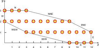
Figure 5: Newton polygon of $\mathscr{A}^{SO}({\bf 3_{1}};x,y;\lambda,t)$.

Face	Face polynomials
N	$\left(1+\lambda t^{3}z\right)\left(1+\lambda^{2}t^{3}z\right)^{2}$
NNE	$\lambda^{5}t^{9}\left(1-\lambda^{5}t^{6}z\right)$
ENE	$\lambda^{10}t^{15}\left(-1+\lambda^{4}tz\right)$
E	$\lambda^{12}t^{12}\left(\lambda^{2}t^{4}-z\right)$
S	$-\lambda^{11}t^{12}(\lambda-z)(-1+z)^{2}$
SSW	$\lambda^{4}t^{4}\left(\lambda^{7}t^{8}-z\right)$
WSW	$-\lambda^{2}\left(\lambda^{2}t^{4}+z\right)$
W	$-\lambda^{2}+z$

Figure 6: Face polynomials of $\mathscr{A}^{SO}({\bf 3_{1}};x,y;\lambda,t)$.

The Newton polygon of the super-$A$-polynomial $\mathscr{A}^{SO}({\bf 3_{1}};x,y;\lambda,t)$ and its face polynomials are shown in Figure 6 and Figure 6. Writing $\mathscr{A}^{SO}({\bf 3_{1}};x,y;\lambda,t)=\sum_{i,j}c_{i,j}(\lambda,t)x^{i}y^{j}$, the Newton polygon is designed by plotting red circles for monomials $c_{ij}\neq 0$ and yellow crosses for monomials at the special limit $c_{ij}(\lambda=1,t=-1)\neq 0$. The faces of the Newton polygons are denoted by the dotted line in Figure 6. For a given face, we rename the monomial coefficients on the face as $c_{k}$. Then, the face polynomial is defined to be $f(z)=\sum_{k}c_{k}z^{k}$. Assuming that the variables $\lambda,t$ are roots of unity, the quantizability condition requires that all roots of $f(z)$ constructed for all faces of the Newton polygon must be roots of unity. Therefore, it is easy to see from Figure 6 that the classical super-$A$-polynomials $\mathscr{A}^{SO}({\bf 3_{1}};x,y;\lambda,t)$ satisfy the necessary condition of quantizability.

At $t=-1$, the super-$A$-polynomial becomes

$$\mathscr{A}^{SO}({\bf 3_{1}};x,y;\lambda,t=-1)$$ (445)

$$= (-1+x\lambda)(y-xy\lambda^{2}-x^{6}\lambda^{7}+x^{7}\lambda^{7})$$

$$\times(-y^{2}+y\lambda^{2}-xy\lambda^{2}+2x^{2}y\lambda^{2}+xy^{2}\lambda^{2}+x^{3}\lambda^{4}-x^{4}\lambda^{4}-2x^{2}y\lambda^{4}-x^{3}y\lambda^{4}+x^{4}y\lambda^{6})~{},$$

while the analysis for the large color behavior of the Kauffman polynomials $F_{[r]}(K;\lambda,q)$ leads to the $\lambda$-deformed $A$-polynomial of $SO$-type

$$A^{SO}({\bf 3_{1}};x,y;\lambda)=y-xy\lambda^{2}-x^{6}\lambda^{7}+x^{7}\lambda^{7}~{}.$$ (447)

Therefore, we can clearly see that $\mathscr{A}^{SO}({\bf 3_{1}};x,y;\lambda,t=-1)\neq A^{SO}({\bf 3_{1}};x,y;\lambda)$ although $\mathscr{A}^{SO}({\bf 3_{1}};x,y;\lambda,t=-1)$ contains $A^{SO}({\bf 3_{1}};x,y;\lambda)$. Furthermore, the $\lambda=1,t=-1$ specialization of the super-$A$-polynomial can be written as

$$\mathscr{A}^{SO}({\bf 3_{1}};x,y;\lambda=1,t=-1) = (x-1)^{3}(1-y)(y-x^{6})(x^{3}+y)~{},$$ (448)

whereas the $PSL(2,\mathbb{C})$ character variety of the trefoil is expressed by

$$A^{PSL(2,\mathbb{C})}({\bf 3_{1}};x,y)=(1-y)(y-x^{6})~{}.$$ (449)

In fact, the large color limit of the $[r]$-colored $\mathfrak{so}(3)$ quantum invariant of the trefoil, i.e. $\mathscr{F}_{[r]}({\bf 3_{1}};\lambda=q^{2},q,t=-1,1)$, provides only the non-abelian branch $y-x^{6}=0$. Hence, ignoring the trivial factor $1-x=0$, the specialization of the super-$A$-polynomial contains not only the abelian branch $1-y=0$ but also the extra non-abelian branch $x^{3}+y=0$. We postpone further study of understanding its meaning to future work.

In the case of the colored $\mathfrak{so}(3)$ quantum invariants, we can find the $q$-difference equation, providing the quantum $PSL(2,\mathbb{C})$ character variety of the trefoil

$$\widehat{A}^{PSL(2,\mathbb{C})}({\bf 3_{1}};\hat{x},\hat{y};q)$$ (450)

$$= (-1+q\hat{x}+\hat{x}^{2}q^{-3}+\hat{x}^{3}q^{-5}-\hat{x}^{3}q^{-2}-\hat{x}^{4}q^{-4}-\hat{x}^{5}q^{-10}+\hat{x}^{6}q^{-9})\hat{y}^{2}$$ (454)

$$-(q^{2}-q^{3}\hat{x}-q^{7}\hat{x}^{2}+q^{8}\hat{x}^{3}-q^{9}\hat{x}^{3}+q^{10}\hat{x}^{4}+q^{12}\hat{x}^{5}-q^{14}\hat{x}^{7}-q^{14}\hat{x}^{8}$$

$$-q^{14}\hat{x}^{9}+q^{15}\hat{x}^{9}+q^{15}\hat{x}^{10}+q^{13}\hat{x}^{11}-q^{14}\hat{x}^{12})\hat{y}$$

$$-(q^{15}\hat{x}^{6}-q^{16}\hat{x}^{7}-q^{24}\hat{x}^{8}+q^{25}\hat{x}^{9}-q^{28}\hat{x}^{9}+q^{29}\hat{x}^{10}+q^{35}\hat{x}^{11}-q^{36}\hat{x}^{12})~{}.$$

A simple computation shows that it reduces to (449) up to trivial factors at $q=1$.

6.2 Figure-eight

Now, let us consider the figure-eight. In the limit (415), the expression (347) behaves as

$$\mathscr{F}_{[r]}({\bf 4_{1}};\lambda,q,t,1)\sim\int e^{\frac{1}{2\hbar}\widetilde{\mathcal{W}}^{SO}({\bf 4_{1}};x,w,v,z)}dwdvdz~{},$$ (455)

with the twisted superpotential

$$\widetilde{\mathcal{W}}^{SO}({\bf 4_{1}};x,w,v,z) = \log\left(\tfrac{z^{2}w}{v^{2}x^{2}}\right)\log{\lambda}-(\log{z})^{2}-\log{z}\log\left(\tfrac{w}{vx^{3}}\right)+\log{\left(\tfrac{w}{x^{2}}\right)}\log{(xv)}$$ (461)

$$+\log\left(\tfrac{z^{2}w}{vx^{2}}\right)\log{t^{2}}-\tfrac{3\pi^{2}}{6}-{\rm Li}_{2}(x)+{\rm Li}_{2}(w)+{\rm Li}_{2}(xz^{-1}w^{-1})$$

$$+{\rm Li}_{2}(v)+{\rm Li}_{2}(zv^{-1})+{\rm Li}_{2}(-\lambda^{2}xz^{-1}w^{-1}t)-{\rm Li}_{2}(-\lambda^{2}xz^{-1}w^{-1}vt)$$

$$-{\rm Li}_{2}(-x^{2}z^{-1}t^{3}\lambda^{2}v)+{\rm Li}_{2}(-t)-{\rm Li}_{2}(-xz^{-1}t)+{\rm Li}_{2}(-\lambda^{2}xt^{3})$$

$$+{\rm Li}_{2}(-\lambda t)-{\rm Li}_{2}(-\lambda xz^{-1}w^{-1}t)+{\rm Li}_{2}(-\lambda xz^{-1}vt^{3})$$

$$-{\rm Li}_{2}(-\lambda x^{2}z^{-2}vw^{-1}t^{3})~{}.$$

In this case, the saddle points are given by the following system of equations:

$$1 = -\tfrac{t^{2}v_{0}w_{0}xz_{0}(-x+w_{0}z_{0})\lambda\left(w_{0}z_{0}+tx\lambda^{2}\right)}{(-1+w_{0})(w_{0}z_{0}+tx\lambda)\left(w_{0}z_{0}^{2}+t^{3}v_{0}x^{2}\lambda\right)\left(w_{0}z_{0}+tv_{0}x\lambda^{2}\right)}~{},$$ (462)

$$1 = -\tfrac{(v_{0}-z_{0})\left(w_{0}z_{0}^{2}+t^{3}v_{0}x^{2}\lambda\right)\left(w_{0}z_{0}+tv_{0}x\lambda^{2}\right)\left(z_{0}+t^{3}v_{0}x^{2}\lambda^{2}\right)}{t^{2}(-1+v_{0})v_{0}w_{0}x^{2}z_{0}^{2}\lambda^{2}\left(z_{0}+t^{3}v_{0}x\lambda\right)}~{},$$ (463)

$$1 = \tfrac{t^{4}v_{0}^{2}w_{0}x^{3}z_{0}^{3}(-x+w_{0}z_{0})\lambda^{2}\left(z_{0}+t^{3}v_{0}x\lambda\right)\left(w_{0}z_{0}+tx\lambda^{2}\right)}{(v_{0}-z_{0})(tx+z_{0})(w_{0}z_{0}+tx\lambda)\left(w_{0}z_{0}^{2}+t^{3}v_{0}x^{2}\lambda\right)^{2}\left(w_{0}z_{0}+tv_{0}x\lambda^{2}\right)\left(z_{0}+t^{3}v_{0}x^{2}\lambda^{2}\right)}~{},$$ (464)

$$y = -\tfrac{(-1+x)(tx+z_{0})(w_{0}z_{0}+tx\lambda)\left(w_{0}z_{0}^{2}+t^{3}v_{0}x^{2}\lambda\right)^{2}\left(w_{0}z_{0}+tv_{0}x\lambda^{2}\right)\left(z_{0}+t^{3}v_{0}x^{2}\lambda^{2}\right)^{2}}{t^{4}v_{0}^{2}w_{0}x^{4}z_{0}^{3}(-x+w_{0}z_{0})\lambda^{2}\left(z_{0}+t^{3}v_{0}x\lambda\right)\left(w_{0}z_{0}+tx\lambda^{2}\right)\left(1+t^{3}x\lambda^{2}\right)}~{}.$$ (465)

With a current desktop computer, it is difficult to solve the above set of the equations for general value of $t$. Thus, we solve it only for the special case $t=-1$ which gives us the $\lambda$-deformed classical $A$-polynomial

$$A^{SO}({\bf 4_{1}};x,y;\lambda)$$ (466)

$$= x^{4}\lambda^{3}(-1+x\lambda^{2})^{3}y^{3}$$ (472)

$$+(1-x)\lambda(-1+x\lambda^{2})^{2}(1-x-x\lambda-x^{2}\lambda-x^{3}\lambda-2x^{2}\lambda^{2}+x^{3}\lambda^{2}+x^{4}\lambda^{2}+2x^{3}\lambda^{3}$$

$$\quad+5x^{4}\lambda^{3}+2x^{5}\lambda^{3}+x^{4}\lambda^{4}+x^{5}\lambda^{4}-2x^{6}\lambda^{4}-x^{5}\lambda^{5}-x^{6}\lambda^{5}-x^{7}\lambda^{5}-x^{7}\lambda^{6}+x^{8}\lambda^{6})y^{2}$$

$$+(1-x)^{2}(-1+x\lambda^{2})(1-x\lambda-x\lambda^{2}-2x^{2}\lambda^{2}-x^{2}\lambda^{3}+2x^{3}\lambda^{3}+x^{3}\lambda^{4}+x^{4}\lambda^{4}-x^{3}\lambda^{5}$$

$$\quad+5x^{4}\lambda^{5}-x^{5}\lambda^{5}+x^{4}\lambda^{6}+x^{5}\lambda^{6}+2x^{5}\lambda^{7}-x^{6}\lambda^{7}-2x^{6}\lambda^{8}-x^{7}\lambda^{8}-x^{7}\lambda^{9}+x^{8}\lambda^{10})y$$

$$+(1-x)^{3}x^{4}\lambda^{6}~{}.$$

In the sequel, one can confirm that the $\lambda$-deformed classical $A$-polynomial $A^{SO}({\bf 4_{1}};x,y;\lambda)$ obeys the quantizability condition, which can be seen in Figure 8 and Figure 8.

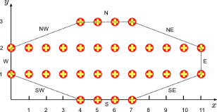
Figure 7: Newton polygon of $A^{SO}({\bf 4_{1}};x,y;\lambda)$.

Face	Face polynomials
N	$\lambda^{3}\left(-1+z\lambda^{2}\right)^{3}$
NE	$-\lambda^{9}\left(-1+z\lambda^{2}\right)$
E	$\lambda^{11}(-1+z\lambda)$
SE	$-\lambda^{6}\left(z-\lambda^{6}\right)$
S	$(-1+z)^{3}\lambda^{6}$
SW	$-z+\lambda^{6}$
W	$-1+z\lambda$
NW	$-\lambda\left(-1+z\lambda^{2}\right)$

Figure 8: Face polynomials of $A^{SO}({\bf 4_{1}};x,y;\lambda)$.

At $\lambda=1$, it reduces to the $A$-polynomial associated to the $PSL(2,\mathbb{C})$ character variety of the figure-eight

$$A^{SO}({\bf 4_{1}};x,y;\lambda=1)$$ (473)

$$= (x-1)^{4}(y-1)^{2}$$ (475)

$$\times(x^{4}-y+2xy+3x^{2}y-2x^{3}y-6x^{4}y-2x^{5}y+3x^{6}y+2x^{7}y-x^{8}y+x^{4}y^{2})~{}.~{}~{}~{}$$

The third factor matches with the non-abelian branch of the $PSL(2,\mathbb{C})$ character variety of the figure-eight. (See Example 1 in §6.0.12. of Champanerkar:2003 .) In fact, the $SL(2,\mathbb{C})$ character variety of the figure-eight is given by

$$A^{SL(2,\mathbb{C})}({\bf 4_{1}};x,y)=(1-y)(x^{4}y^{2}+(x^{8}-x^{6}-2x^{4}-x^{2}+1)y+x^{4})~{}.$$ (476)

Therefore, $A^{SO}({\bf 4_{1}};x,y;\lambda=1)$ is equal to $A^{SL(2,\mathbb{C})}({\bf 4_{1}};x^{1/2},y^{1/2})A^{SL(2,\mathbb{C})}({\bf 4_{1}};x^{1/2},-y^{1/2})$ up to the trivial factors as stated in (411). In addition, we can obtain the $q$-difference equation for the colored $\mathfrak{so}(3)$ quantum invariants shown in Table 5.

7 3d/3d correspondence

One of the most remarkable developments in recent years has been the program of studying a duality arising from the compactification of the 6d (2,0) superconformal field theory on a certain manifold. Particularly, the partially twisted compactification of the 6d (2,0) theory with Lie algebra $\mathfrak{g}$ on a 3-manifold $M$ leads to a 3d $\mathcal{N}=2$ supersymmetric gauge theory $T_{\mathfrak{g}}[M]$, yielding deep relations between the geometry of the 3-manifold $M$ and the properties of the theory $T_{\mathfrak{g}}[M]$ Dimofte:2010tz ; Terashima:2011qi ; Dimofte:2011ju ; Dimofte:2011py . The relation can be recapitulated by the statement that the partition function of $T_{\mathfrak{g}}[M]$ on the squashed sphere $S^{3}_{b}$ or the superconformal index of $T_{\mathfrak{g}}[M]$ is equal to the partition function of $G_{\mathbb{C}}$ Chern-Simons theory on $M$. As a consequence, the moduli space of flat $G_{\mathbb{C}}$ connections on $M$ is identified with the moduli space of supersymmetric vacua in the dual 3d gauge theory $T_{\mathfrak{g}}[M]$. This correspondence has been lately placed on a rigorous footing by the localization technique Yagi:2013fda ; Lee:2013ida ; Cordova:2013cea .

The explicit IR descriptions of $T_{\mathfrak{sl}(2)}[M]$ for a large class of 3-manifolds $M$ have been established by abelian $\mathcal{N}=2$ gauge theories, with possibly non-perturbative superpotentials that preserve $U(1)_{R}$ Dimofte:2011ju ; Dimofte:2011py . In particular, the cases in which a 3-manifold $M$ is a knot complement $S^{3}\backslash K$ have been intensively investigated Dimofte:2011ju ; Dimofte:2011py ; Beem:2012mb ; Dimofte:2013lba ; Fuji:2012pi . Moreover, in this setting, the relation between “holomorphic blocks” $B^{\alpha}(x;q)$ and colored Jones polynomials has been investigated in Beem:2012mb . Roughly speaking, a holomorphic block $B^{\alpha}(x;q)$ is the partition function on $S^{1}\times\mathbb{R}$, labelled by a choice of vacuum $\alpha$ at the asymptotic boundary of spatial $\mathbb{R}^{2}$ whose form is

$$B^{\alpha}(x;q)\,\sim\,\mbox{Tr}_{\mathcal{H}(\mathbb{R}^{2};\alpha)}(-1)^{R}e^{-\beta H}q^{-J+\frac{R}{2}}x^{e}\,,$$ (477)

with fugacity $x$ for the $U(1)$ flavor symmetry. Note that the fugacity $x$ is identified with the holonomy eigenvalue $x$ of the gauge connection along the meridian of the tubular neighborhood of $K$ in $SL(2,\mathbb{C})$ Chern-Simons theory. Given an abelian $\mathcal{N}=2$ gauge theory, the holomorphic block can be schematically expressed as

$$B^{\alpha}(x;q)\;\sim\;\int_{\Gamma^{\alpha}}\frac{dz}{z}\,\big{[}\theta(w;q)...\big{]}B_{\Delta}(w_{1};q)\cdots B_{\Delta}(w_{N};q)\,,$$ (478)

where we choose the appropriate integration cycle $\Gamma^{\alpha}\subset(\mathbb{C}^{\times})^{s}$, with $s$ being the number of the $U(1)$ gauge groups. The variables $z\in(\mathbb{C}^{*})^{s}$ are complexified scalars in the gauge multiplets, and each chiral multiplet contributes a single block

$$B_{\Delta}(w;q)=\sum_{n=0}^{\infty}\frac{w^{-n}}{(q^{-1};q^{-1})_{n}}\,,$$ (479)

to the integrand. Note that the parameter $w_{i}=w_{i}(z,x)$ depends on the scalars $z$ and the fugacity $x$. Here, the theta-functions $\theta(w;q)$ encode contributions of Chern-Simons and Fayet-Iliopoulos (FI) terms. Then, it was observed in Beem:2012mb that the holomorphic block $B(x=q^{2r};q)$ of $T_{\mathfrak{sl}(2)}[S^{3}\backslash K]$ at $x=q^{2r}$ coincides with the stable limit of the colored Jones polynomial $J_{[r]}(K;q)$. Nevertheless, the holomorphic block $B(x=q^{2r};q)$ of $T_{\mathfrak{sl}(2)}[S^{3}\backslash K]$ does not reproduce the colored Jones polynomial exactly. This appears to be related to the fact that the way the theory $T_{\mathfrak{sl}(2)}[S^{3}\backslash K]$ is constructed captures only the non-abelian branch, but not the abelian branch of the $SL(2,\mathbb{C})$ character variety. Equivalently, this can be rephrased that the large color limit of colored Jones polynomials provides only the non-abelian branch.

On the other hand, as we have seen in §6, a super-$A$-polynomial encodes much richer information than an ordinary $A$-polynomial. The most important fact is that it intrinsically encompasses the abelian branch. Thus, it seems more appropriate to consider the 3d/3d correspondence in this setting. As discussed in Fuji:2012nx ; Fuji:2012pi , the parameters $a$ or $\lambda$, and $t$ can be interpreted as fugacities in the index for certain global symmetries $U(1)_{\text{bulk}}$ and $U(1)_{F}$ in the context of $\mathcal{N}=2$ gauge theory. Thus, super-$A$-polynomials carry important information about $\mathcal{N}=2$ gauge theories with those symmetries. Taking into account these features, it would certainly be interesting to elucidate the relation between the “refined” holomorphic blocks and the Poincaré polynomials of knot homology Chung:2013 .

As in the $\mathfrak{sl}(2)$ case, the IR descriptions of $T_{\mathfrak{so}(3)}[S^{3}\backslash K]$ can be constructed by abelian $\mathcal{N}=2$ gauge theories. In fact, the Kaluza-Klein reduction on $S^{1}$ with $q\to 1$ brings (478) to the form given in (421) and (455). In the leading contribution, a single block $B_{\Delta}$ yields a dilogarithm (${\rm Li}_{2}$) to the twisted superpotential. Hence, each dilogarithm (${\rm Li}_{2}$) term in the twisted superpotential $\widetilde{\mathcal{W}}$ expresses the contribution from a chiral field $\phi_{i}$. In (421) and (455), the parameters $w$, $v$ and $z$ can be interpreted as scalars in $U(1)$ gauge multiplets. Therefore, if the $j$-th dilogarithm term in $\widetilde{\mathcal{W}}$ is $\pm{\rm Li}_{2}\left(x^{n_{1}}(-t)^{n_{2}}a^{n_{3}}z_{i}^{n_{4}}\right)$, then the chiral field $\phi_{j}$ will have charges $\pm n_{1}$, $\pm n_{2}$, $\pm n_{3}$, $\pm n_{4}$ respectively under the $U(1)_{x}$, $U(1)_{F}$, $U(1)_{\text{bulk}}$ global symmetries and $U(1)_{z_{i}}$ gauge groups. In addition, the theta-functions reduces to the term $-\log x_{i}\cdot\log z_{j}$ for the FI coupling and the term $\frac{k_{ij}}{2}\,\log z_{i}\cdot\log z_{j}$ for the supersymmetric Chern-Simons coupling $\frac{k_{ij}}{4\pi}\int A_{i}\wedge dA_{j}$. Using this dictionary, one can read off the theory $T_{\mathfrak{so}(3)}[S^{3}\backslash{\bf 3_{1}}]$ and $T_{\mathfrak{so}(3)}[S^{3}\backslash{\bf 4_{1}}]$ where the $U(1)$ charges of matter contents are depicted in Table 3 and Table 4.

$$\begin{array}[]{|l|c|c|c|c|c|c|c|c|c|c|c|c|}\hline\cr&\phi_{1}&\phi_{2}&\phi_{3}&\phi_{4}&\phi_{5}&\phi_{6}&\phi_{7}&\phi_{8}&\phi_{9}&\phi_{10}&\phi_{11}&\text{Parameter}\\ \hline\cr U(1)_{\rm gauge}&0&0&1&0&-1&0&0&0&1&0&0&z\\ U(1)_{\rm gauge}&0&0&0&1&-1&0&0&0&0&0&1&w\\ U(1)_{\rm gauge}&0&1&-1&0&0&0&-1&0&0&0&0&v\\ U(1)_{\rm global}&-1&0&0&0&1&1&-1&0&-1&0&0&x\\ U(1)_{\rm bulk}&0&0&0&0&0&2&-2&0&0&1&-1&\lambda\\ U(1)_{\rm F}&0&0&0&0&0&3&-3&1&-1&1&-1&t\\ \hline\cr\end{array}$$

Table 3: $U(1)$ charges of the chiral fields corresponding to the twisted superpotential $\widetilde{\mathcal{W}}^{SO}({\bf 3_{1}};x,w,v,z)$.

$$\begin{array}[]{|l|c|c|c|c|c|c|c|c|c|c|c|c|c|c|c|c|c|c|}\hline\cr&\phi_{1}&\phi_{2}&\phi_{3}&\phi_{4}&\phi_{5}&\phi_{6}&\phi_{7}&\phi_{8}&\phi_{9}&\phi_{10}&\phi_{11}&\phi_{12}&\phi_{13}&\phi_{14}&\phi_{15}&\text{Parameter}\\ \hline\cr U(1)_{\rm gauge}&0&0&-1&0&1&-1&1&1&0&1&0&0&1&-1&2&z\\ U(1)_{\rm gauge}&0&1&-1&0&0&-1&1&0&0&0&0&0&1&0&1&w\\ U(1)_{\rm gauge}&0&0&0&1&-1&0&-1&-1&0&0&0&0&0&1&-1&v\\ U(1)_{\rm global}&-1&0&1&0&0&1&-1&-2&0&-1&1&0&-1&1&-2&x\\ U(1)_{\rm bulk}&0&0&0&0&0&2&-2&-2&0&0&2&1&-1&1&-1&\lambda\\ U(1)_{\rm F}&0&0&0&0&0&1&-1&-3&1&-1&3&1&-1&3&-3&t\\ \hline\cr\end{array}$$

Table 4: $U(1)$ charges of the chiral fields corresponding to the twisted superpotential $\widetilde{\mathcal{W}}^{SO}({\bf 4_{1}};x,w,v,z)$.

8 Future directions

The study on the structure of the $[r]$-colored Kauffman homology that we have implemented raises several questions. Although we focused on thin knots of the simplest class so far, it would be desirable to study whether these structural properties hold for the Kauffman homology of thick knots. However, the size of colored Kauffman homology for thick knots would be too large to study with our current technique. Nevertheless, it is worth making the following comments. Given the uncolored Kauffman homology of the $(3,4)$-torus knot $T_{3,4}$ (Appendix B in Gukov:2011ry ), its uncolored $\mathfrak{so}(4)$ homology should be isomorphic to the homology with respect to the $d_{4}$ differential. However, if we use the differential whose $(\lambda,q,t_{r},t_{c})$-degree is $\deg d_{4}=(-1,3,-1,-1)$ as in (124), the homology $H_{*}(\mathscr{H}^{\rm Kauffman}_{\yng(1)}(T_{3,4}),d_{4})$ would be 41-dimensional while the uncolored $\mathfrak{so}(4)$ homology of $T_{3,4}$ should be 25-dimensional, which follows from the 5-dimensional uncolored $\mathfrak{sl}(2)$ homology of $T_{3,4}$. This indicates that one has to take into account the spectral sequence Rasmussen:2006 for the $d_{4}$ differential in the case of thick knots.

Another important problem concerns the interpretation of the differentials inherent in colored Kauffman homology. In Gukov:2005qp , the differentials in uncolored Kauffman homology are elucidated by the deformations of the Landau-Ginzburg potential in B-model. One way to relate the colored Kauffman homology to the Landau-Ginzburg B-model is the algebraic model proposed in Gorsky:2013jxa . In this model, the colored HOMFLY homology of a torus knot is identified with a space of differential forms on a certain reduced moduli space. This description is certainly suitable for the interpretation in terms of the Landau-Ginzburg model. Hence, the route via the algebraic model may connect to the explanation of the differentials in terms of the Landau-Ginzburg B-model .

Furthermore, it was observed in Gorsky:2013jxa that the colored differentials present in the HOMFLY homology can be associated with the representations of the Lie superalgebra $\mathfrak{sl}(n|m)$. Therefore, it would be intriguing to consider the relation to Lie superalgebra and its physical meaning in the context of the colored Kauffman homology.

It is also worthwhile to find a new way to look at the $\lambda$-deformed $A$-polynomials of $SO$-type. It is conjectured in Aganagic:2012jb that the $a$-deformed $A$-polynomials of $SU$-type can be identified with the augmentation polynomials of knot contact homology Ng:2010 ; Ekholm:2010 . This conjecture has been verified in the cases of the $(2,2p+1)$-torus knots Fuji:2012nx and the twist knots Fuji:2012pi ; Nawata:2012pg . It is natural to ask whether or not one can construct augmentation polynomials in knot contact homology analogous to the $\lambda$-deformed $A$-polynomials of $SO$-type.

Finally, one may be interested in extracting information about quantum $6j$-symbols for $U_{q}(\mathfrak{so}(N))$ from the expressions for the invariants of the trefoil and the figure-eight obtained in §5 as done in Nawata:2013ppa for $U_{q}(\mathfrak{sl}(N))$. For this purpose, the relations from representation theory will be also useful. In fact, quantum $6j$-symbols for $U_{q}(\mathfrak{so}(N))$ would enable us to evaluate colored $\mathfrak{so}(N)$ quantum invariants for any knot. The feasibility of this approach is currently under investigation.

Appendix A Conventions and notations

Polynomial invariants

$J^{\mathfrak{g}}_{R}(K;q)$	The reduced $\mathfrak{g}$ quantum invariant of a knot $K$ colored by a representation $R$ of $\mathfrak{g}$
$\overline{J}^{\mathfrak{g}}_{R}(K;q)$	The unreduced $\mathfrak{g}$ quantum invariant of a knot $K$ colored by a representation $R$ of $\mathfrak{g}$
$P_{R}(K;a,q)$	The reduced HOMFLY polynomial of a knot $K$ colored by a representation $R$
$\overline{P}_{R}(K;a,q)$	The unreduced HOMFLY polynomial of a knot $K$ colored by a representation $R$
$\overline{P}_{(R,S)}(K;a,q)$	The unreduced HOMFLY polynomial of a knot $K$ colored by a composite representation $(R,S)$
$F_{R}(K;\lambda,q)$	The reduced Kauffman polynomial of a knot $K$ colored by a representation $R$
$\overline{F}_{R}(K;\lambda,q)$	The unreduced Kauffman polynomial of a knot $K$ colored by a representation $R$

Knot homology

$(\mathscr{H}^{\rm HOMFLY}_{R}(K))_{i,j,k,\ell}$	The reduced quadruply-graded HOMFLY homology colored by a representation $R$ with $(a,q,t_{r},t_{c})$-gradings
$(\widetilde{}\mathscr{H}^{\rm HOMFLY}_{R}(K))_{i,j,k,\ell}$	The reduced quadruply-graded HOMFLY homology colored by a representation $R$ with $(a,Q,t_{r},t_{c})$-gradings
$H_{*}(\mathscr{H}^{\rm HOMFLY}_{R}(K),d)_{i,j,k,\ell}$	The homology with respect to a differential $d$ acting on $(\mathscr{H}^{\rm HOMFLY}_{R}(K))_{i,j,k,.\ell}$ with $(a,q,t_{r},t_{c})$-gradings
$H_{*}(\widetilde{}\mathscr{H}^{\rm HOMFLY}_{R}(K),d)_{i,j,k,\ell}$	The homology with respect to a differential $d$ acting on $(\widetilde{}\mathscr{H}^{\rm HOMFLY}_{R}(K))_{i,j,k,.\ell}$ with $(a,Q,t_{r},t_{c})$-gradings
$(\mathscr{H}^{\rm Kauffman}_{R}(K))_{i,j,k,.\ell}$	The reduced quadruply-graded Kauffman homology colored by a representation $R$ with $(\lambda,q,t_{r},t_{c})$-gradings
$(\widetilde{}\mathscr{H}^{\rm Kauffman}_{R}(K))_{i,j,k,\ell}$	The reduced quadruply-graded Kauffman homology colored by a representation $R$ with $(\lambda,Q,t_{r},t_{c})$-gradings
$H_{*}(\mathscr{H}^{\rm Kauffman}_{R}(K),d)_{i,j,k,\ell}$	The homology with respect to a differential $d$ acting on $(\mathscr{H}^{\rm Kauffman}_{R}(K))_{i,j,k,.\ell}$ with $(\lambda,q,t_{r},t_{c})$-gradings
$H_{*}(\widetilde{}\mathscr{H}^{\rm Kauffman}_{R}(K),d)_{i,j,k,\ell}$	The homology with respect to a differential $d$ acting on $(\widetilde{}\mathscr{H}^{\rm Kauffman}_{R}(K))_{i,j,k,.\ell}$ with $(\lambda,Q,t_{r},t_{c})$-gradings

Poincaré polynomials

$$\mathscr{P}_{R}(K;a,q,t_{r},t_{c}) := \sum_{i,j,k,\ell}a^{i}q^{j}t_{r}^{k}t_{c}^{\ell}~{}\dim\;(\mathscr{H}^{\rm HOMFLY}_{R}(K))_{i,j,k,\ell}$$

$$\widetilde{}\mathscr{P}_{R}(K;a,Q,t_{r},t_{c}) := \sum_{i,j,k,\ell}a^{i}Q^{j}t_{r}^{k}t_{c}^{\ell}~{}\dim\;(\widetilde{}\mathscr{H}^{\rm HOMFLY}_{R}(K))_{i,j,k,\ell}$$

$$\mathscr{P}(\mathscr{H}^{\rm HOMFLY}_{R}(K),d)(a,q,t_{r},t_{c}) := \sum_{i,j,k,\ell}a^{i}q^{j}t_{r}^{k}t_{c}^{\ell}~{}\dim H_{*}(\mathscr{H}^{\rm HOMFLY}_{R}(K),d)_{i,j,k,\ell}$$

$$\widetilde{}\mathscr{P}(\widetilde{}\mathscr{H}^{\rm HOMFLY}_{R}(K),d)(a,Q,t_{r},t_{c}) := \sum_{i,j,k,\ell}a^{i}Q^{j}t_{r}^{k}t_{c}^{\ell}~{}\dim H_{*}(\widetilde{}\mathscr{H}^{\rm HOMFLY}_{R}(K),d)_{i,j,k,\ell}$$

$$\mathscr{F}_{R}(K;\lambda,q,t_{r},t_{c}) := \sum_{i,j,k,\ell}\lambda^{i}q^{j}t_{r}^{k}t_{c}^{\ell}~{}\dim\;(\mathscr{H}^{\rm Kauffman}_{R}(K))_{i,j,k,\ell}$$

$$\widetilde{}\mathscr{F}_{R}(K;\lambda,Q,t_{r},t_{c}) := \sum_{i,j,k,\ell}\lambda^{i}Q^{j}t_{r}^{k}t_{c}^{\ell}~{}\dim\;(\widetilde{}\mathscr{H}^{\rm Kauffman}_{R}(K))_{i,j,k,\ell}$$

$$\mathscr{F}(\mathscr{H}^{\rm Kauffman}_{R}(K),d)(\lambda,q,t_{r},t_{c}) := \sum_{i,j,k,\ell}\lambda^{i}q^{j}t_{r}^{k}t_{c}^{\ell}~{}\dim H_{*}(\mathscr{H}^{\rm Kauffman}_{R}(K),d_{N})_{i,j,k,\ell}$$

$$\widetilde{}\mathscr{F}(\widetilde{}\mathscr{H}^{\rm Kauffman}_{R}(K),d)(\lambda,Q,t_{r},t_{c}) := \sum_{i,j,k,\ell}\lambda^{i}Q^{j}t_{r}^{k}t_{c}^{\ell}~{}\dim H_{*}(\widetilde{}\mathscr{H}^{\rm Kauffman}_{R}(K),d)_{i,j,k,\ell}$$

$A$-polynomials

$A^{SL(2,\mathbb{C})}(K;x,y)$	The $SL(2,\mathbb{C})$ character variety of the complement of a knot $K$ in $S^{3}$
$A^{PSL(2,\mathbb{C})}(K;x,y)$	The $PSL(2,\mathbb{C})$ character variety of the complement of a knot $K$ in $S^{3}$
$\widehat{A}^{PSL(2,\mathbb{C})}(K;\hat{x},\hat{y};q)$	The quantum $PSL(2,\mathbb{C})$ character variety of the complement of a knot $K$ in $S^{3}$
$A^{SU}(K;x,y;a)$	The $a$-deformed $A$-polynomial of $SU$-type for a knot $K$
$A^{SO}(K;x,y;\lambda)$	The $\lambda$-deformed $A$-polynomial of $SO$-type for a knot $K$
$\widehat{A}^{SO}(K;\hat{x},\hat{y};\lambda,q)$	The quantum $\lambda$-deformed $A$-polynomial of $SO$-type for a knot $K$
$\mathscr{A}^{SU}(K;x,y;a,t)$	The super-$A$-polynomial of $SU$-type for a knot $K$
$\mathscr{A}^{SO}(K;x,y;\lambda,t)$	The super-$A$-polynomial of $SO$-type for a knot $K$

Appendix B Integrality conjecture for Kauffman polynomials

In this appendix, we check the integrality conjecture proposed by Mariño Marino:2009mw for Kauffman polynomials using the invariants of the figure-eight. This is the first non-trivial check of the integrality conjecture for a non-torus knot that provides an indirect evidence for geometric transition in the presence of an orientifold Sinha:2000ap .

Similar to Ooguri-Vafa reformulated polynomials, we can determine reformulated invariants $g_{R}(K;\lambda,q)$ with integrality structure using unreduced colored Kauffman polynomials and unreduced colored HOMFLY polynomials. Although the Ooguri-Vafa-Labastida-Mariño conjecture for $U(N)$ invariants was proven in Liu:2007kv ; Liu:2010zr , the Mariño’s conjecture Marino:2009mw still remains open. The colored Kauffman polynomials for knots appear in writing the expectation value of the Ooguri-Vafa operator

$$Z_{CS}^{SO/Sp}(K;\lambda,q,v)=\sum_{R}{\overline{F}}_{R}(K;\lambda,q)s_{R}(v)~{},$$ (480)

in the A-model topological strings on an orientifolded conifold background where $s_{R}(v)$ are the Schur polynomials in variable $v$. As explained in (53), the topological string partition function in this background receives the contributions from the oriented and unoriented sectors Bouchard:2004iu ; Bouchard:2004ri ; Borhade:2005pw ; Marino:2009mw . The oriented topological string amplitude involves colored HOMFLY polynomials of knots carrying composite representations $(R,S)$ Marino:2009mw

$$\log\left[\sum_{R,S}{\overline{P}}_{(R,S)}(K;a,q)s_{R}(v)s_{S}(v)\right]=\sum_{\widetilde{R}}\sum_{d=1}^{\infty}\frac{1}{d}h_{\widetilde{R}}(a^{d},q^{d})s_{\widetilde{R}}(v^{d})~{}.$$ (481)

It is straightforward to obtain the explicit expressions up to double boxes

$$h_{\yng(1)}(K;a,q) = 2\overline{P}_{\yng(1)}(K;a,q)~{},$$ (482)

$$h_{\yng(2)}(K;a,q) = 2\overline{P}_{\yng(2)}(K;a,q)+\overline{P}_{(\yng(1),\yng(1))}(K;a,q)-2\overline{P}_{\yng(1)}(K;a,q)^{2}-\overline{P}_{\yng(1)}(K;a^{2},q^{2})~{},$$ (483)

$$h_{\yng(1,1)}(K;a,q) = 2\overline{P}_{\yng(1,1)}(K;a,q)+\overline{P}_{(\yng(1),\yng(1))}(K;a,q)-2\overline{P}_{\yng(1)}(K;a,q)^{2}+\overline{P}_{\yng(1)}(K;a^{2},q^{2})~{}.$$ (484)

The reformulated invariant is expected to obey the Ooguri-Vafa integrality structure

$$h_{R}(K;a,q)=\frac{1}{q-q^{-1}}\sum_{\beta,s}N_{R,\beta,s}(K)a^{\beta}q^{s}~{},$$ (485)

where $N_{R,\beta,s}$ are integers. The check of this conjecture for the figure-eight requires the HOMFLY polynomials colored by composite representations. Fortunately, the colored HOMFLY polynomial of the figure-eight colored by composite representation $(\yng(1),\yng(1))$ is given in p.25 of Hadji:2006

$${\overline{P}}_{(\yng(1),\yng(1))}({\bf 4_{1}})$$ (486)

$$= 3-2z^{2}-6z^{4}-2z^{6}+\left(-2-z^{2}+2z^{4}+z^{6}\right)\left(\tfrac{1}{\lambda^{2}}+\lambda^{2}\right)+\left(1+2z^{2}+z^{4}\right)\left(\tfrac{1}{\lambda^{4}}+\lambda^{4}\right)$$ (487)

$$= 11-\tfrac{2}{q^{6}}+\tfrac{6}{q^{4}}-\tfrac{8}{q^{2}}-8q^{2}+6q^{4}-2q^{6}+\lambda^{-4}\left(3+\tfrac{1}{q^{4}}-\tfrac{2}{q^{2}}-2q^{2}+q^{4}\right)$$ (490)

$$+\lambda^{4}\left(3+\tfrac{1}{q^{4}}-\tfrac{2}{q^{2}}-2q^{2}+q^{4}\right)+\lambda^{-2}\left(-8+\tfrac{1}{q^{6}}-\tfrac{4}{q^{4}}+\tfrac{6}{q^{2}}+6q^{2}-4q^{4}+q^{6}\right)$$

$$+\lambda^{2}\left(-8+\tfrac{1}{q^{6}}-\tfrac{4}{q^{4}}+\tfrac{6}{q^{2}}+6q^{2}-4q^{4}+q^{6}\right),$$

where $z=q-q^{-1}$. Using this data, we can verify the expected form (485) for the figure-eight upto two boxes:

$$h_{\yng(2)}({\bf 4_{1}};a,q) = -\frac{1}{a^{6}q^{7}(q-q^{-1})}(-a^{4}+2a^{6}-a^{8}-2a^{2}q^{2}+5a^{4}q^{2}-4a^{6}q^{2}+a^{8}q^{2}+3q^{4}$$ (495)

$$-6a^{2}q^{4}+2a^{4}q^{4}+2a^{6}q^{4}-2a^{10}q^{4}+a^{12}q^{4}-q^{6}+2a^{2}q^{6}+2a^{4}q^{6}-5a^{6}q^{6}$$

$$-2a^{8}q^{6}+4a^{10}q^{6}-a^{12}q^{6}+q^{8}-4a^{2}q^{8}+2a^{4}q^{8}+5a^{6}q^{8}-2a^{8}q^{8}-2a^{10}q^{8}$$

$$+a^{12}q^{8}-q^{10}+2a^{2}q^{10}-2a^{6}q^{10}-2a^{8}q^{10}+6a^{10}q^{10}-3a^{12}q^{10}-a^{4}q^{12}$$

$$+4a^{6}q^{12}-5a^{8}q^{12}+2a^{10}q^{12}+a^{4}q^{14}-2a^{6}q^{14}+a^{8}q^{14})~{},$$

$$h_{\yng(1,1)}({\bf 4_{1}};a,q) = -\frac{1}{a^{6}q^{7}(q-q^{-1})}(-a^{4}+2a^{6}-a^{8}+a^{4}q^{2}-4a^{6}q^{2}+5a^{8}q^{2}-2a^{10}q^{2}+q^{4}$$ (500)

$$-2a^{2}q^{4}+2a^{6}q^{4}+2a^{8}q^{4}-6a^{10}q^{4}+3a^{12}q^{4}-q^{6}+4a^{2}q^{6}-2a^{4}q^{6}-5a^{6}q^{6}$$

$$+2a^{8}q^{6}+2a^{10}q^{6}-a^{12}q^{6}+q^{8}-2a^{2}q^{8}-2a^{4}q^{8}+5a^{6}q^{8}+2a^{8}q^{8}-4a^{10}q^{8}$$

$$+a^{12}q^{8}-3q^{10}+6a^{2}q^{10}-2a^{4}q^{10}-2a^{6}q^{10}+2a^{10}q^{10}-a^{12}q^{10}$$

$$+2a^{2}q^{12}-5a^{4}q^{12}+4a^{6}q^{12}-a^{8}q^{12}+a^{4}q^{14}-2a^{6}q^{14}+a^{8}q^{14})~{}.$$

Subtracting the oriented contribution from the free energy $\log Z_{CS}^{SO/Sp}(K)$, one can write the contribution from the unoriented sector invoving the reformulated polynomials $g_{R}(K;\lambda,q)$

$$\log Z_{CS}^{SO/Sp}(K;\lambda,q,v)-\frac{1}{2}\log\left[\sum_{R,S}{\overline{P}}_{(R,S)}(K;\lambda,q)s_{R}(v)s_{S}(v)\right]=\sum_{\widetilde{R}}\sum_{d:{\rm odd}}{1\over d}g_{\widetilde{R}}(K;\lambda^{d},q^{d})s_{\widetilde{R}}(v^{d})~{},$$ (501)

where the variable $\lambda$ is substituted for the variable $a$ in the colored HOMFLY polynomials. For representations up to two boxes, the above equation gives

$$g_{\yng(1)}(K;\lambda,q) = {\overline{F}}_{\yng(1)}(K;\lambda,q)-{\overline{P}}_{\yng(1)}(K;\lambda,q)~{},$$ (502)

$$g_{\yng(2)}(K;\lambda,q) = {\overline{F}}_{\yng(2)}(K;\lambda,q)-\tfrac{1}{2}{\overline{F}}_{\yng(1)}(K;\lambda,q)^{2}-{\overline{P}}_{\yng(2)}(K;\lambda,q)+{\overline{P}}_{\yng(1)}(K;\lambda,q)^{2}-\tfrac{1}{2}{\overline{P}}_{(\yng(1),\yng(1))}(K;\lambda,q)~{},$$ (503)

$$g_{\yng(1,1)}(K;\lambda,q) = {\overline{F}}_{\yng(1,1)}(K;\lambda,q)-\tfrac{1}{2}{\overline{F}}_{\yng(1)}(K;\lambda,q)^{2}-{\overline{P}}_{\yng(1,1)}(K;\lambda,q)+{\overline{P}}_{\yng(1)}(K;\lambda,q)^{2}-\tfrac{1}{2}{\overline{P}}_{(\yng(1),\yng(1))}(K;\lambda,q)~{}.$$ (504)

The reformulated invariants $g_{R}(K;\lambda,q)$ have been obtained for many framed torus knots/links Marino:2009mw ; Paul:2010qu ; Stevan:2010jh . Nevertheless, no calculation has been implemented for the reformulated invariants of non-torus knots/links beyond a single box $\yng(1)$ because it is difficult at present to evaluate colored Kauffman polynomials and colored HOMFLY polynomials with composite representations.

With the colored Kauffman polynomial (347) of the figure-eight, we can calculate the reformulated polynomials $g_{\yng(2)}({\bf 4_{1}};\lambda,q)$ and $g_{\yng(1,1)}({\bf 4_{1}};\lambda,q)$:

$$g_{\yng(2)}({\bf 4_{1}};\lambda,q) = \tfrac{1}{\lambda^{6}q^{12}}(-1+\lambda)(1+\lambda)(\lambda-q)(\lambda+q)(-1+\lambda q)(1+\lambda q)$$ (509)

$$\times(-1+\lambda q+\lambda^{2}q^{4}-\lambda^{3}q^{5}-q^{6}+\lambda q^{7}+q^{8}-2\lambda^{2}q^{8}+\lambda^{4}q^{8}-\lambda^{6}q^{8}+\lambda^{3}q^{9}$$

$$+2\lambda^{2}q^{10}-2\lambda^{4}q^{10}-\lambda^{3}q^{11}+q^{12}-\lambda^{2}q^{12}+2\lambda^{4}q^{12}-\lambda^{6}q^{12}-\lambda^{5}q^{13}+\lambda^{6}q^{14}$$

$$+\lambda^{3}q^{15}-\lambda^{4}q^{16}-\lambda^{5}q^{19}+\lambda^{6}q^{20})~{},$$

$$g_{\yng(1,1)}({\bf 4_{1}};\lambda,q) = \tfrac{1}{q^{12}\lambda^{6}}(q-\lambda)(-1+\lambda)(1+\lambda)(q+\lambda)(-1+q\lambda)(1+q\lambda)$$ (513)

$$(-q^{8}g-q^{12}+q^{14}+q^{20}+q^{13}\lambda+q^{19}\lambda+q^{8}\lambda^{2}-2q^{10}\lambda^{2}+2q^{12}\lambda^{2}$$

$$-q^{16}\lambda^{2}+q^{5}\lambda^{3}-q^{9}\lambda^{3}+q^{11}\lambda^{3}-q^{15}\lambda^{3}+q^{4}\lambda^{4}-2q^{8}\lambda^{4}+2q^{10}\lambda^{4}$$

$$-q^{12}\lambda^{4}-q\lambda^{5}-q^{7}\lambda^{5}-\lambda^{6}-q^{6}\lambda^{6}+q^{8}\lambda^{6}+q^{12}\lambda^{6})~{}.$$

The above two reformulated polynomials agrees with the expected integrality structure $g_{R}(K;\lambda,q)\propto\sum_{\beta,s}N_{R,\beta,s}\lambda^{\beta}(K)q^{s}$.

To see the connection with the configurations of the M2-branes explained in §3.1, one can define the partition $\mu$ from the winding number $w=(w_{1},\cdots,w_{h})$ as follows: the $i$-th entry of $\mu$ is the number of $w_{j}$s that take the value $i$. Then, one can relate the winding number $w$ basis to the representation $R$ basis by

$$\mbox{Tr}_{R}(U)=\sum_{\mu}\frac{\chi_{R}(C_{\mu})}{z_{\mu}}\prod_{j=1}^{\infty}(\mbox{Tr}~{}U^{j})^{\mu_{j}}~{},$$ (514)

where $z_{\mu}=\prod_{i}i^{\mu_{i}}\mu_{i}!$. Note that we denote by $\chi_{R}(C_{\mu})$ the character of the symmetric group representation $R$ in the conjugacy class $C_{\mu}$ associated to the partition $\mu$ such that $\sum_{j}j\mu_{j}=|R|$. Thus, to obtain BPS integer coefficients, we need to change the basis in such a way that

$${\hat{h}}_{R}(K;a,q) = \sum_{S}(M^{-1})_{RS}~{}h_{S}(K;a,q)~{},$$ (515)

$${\hat{g}}_{R}(K;\lambda,q) = \sum_{S}(M^{-1})_{RS}~{}g_{S}(K;\lambda,q)~{},$$ (516)

where the matrix $M_{RS}$ is an invertible matrix given by

$$M_{RS}=\sum_{\mu}{1\over z_{\mu}}\chi_{R}(C_{\mu})\chi_{S}(C_{\mu}){\prod_{i=1}^{\ell({\mu})}(q^{i}-q^{-i})^{\mu_{i}}\over{q-q^{-1}}}~{}.$$ (517)

Writing with the variable $z=q-q^{-1}$ instead of the variable $q$, one can extract BPS integer degeneracies $\widehat{N}^{c}_{R;g,\beta}(K)$ from the reformulated invariants ${\hat{h}}_{R}$ and ${\hat{g}}_{R}$ Marino:2009mw

$$\hat{h}_{R}(K;\lambda,z) = \sum_{g\geq 0}\sum_{\beta\in\mathbb{Z}}\left(\widehat{N}^{c=0}_{R;g,\beta}(K)z^{2g-1}\lambda^{\beta}\right)~{},$$ (518)

$$\hat{g}_{R}(K;\lambda,z) = \sum_{g\geq 0}\sum_{\beta\in\mathbb{Z}}\left(\widehat{N}^{c=1}_{R;g,\beta}(K)z^{2g}\lambda^{\beta}+\widehat{N}^{c=2}_{R;g,\beta}(K)z^{2g+1}\lambda^{\beta}\right)~{}.$$ (519)

Using the inverse of the matrix $M_{RS}$, we can write

$$\hat{h}_{\yng(2)}({\bf 4_{1}};a,q) = \frac{q~{}h_{\yng(2)}({\bf 4_{1}};a,q)+q^{-1}h_{\yng(1,1)}({\bf 4_{1}};a,q)}{q^{2}-q^{-2}}$$ (520)

$$= \frac{1}{a^{6}q^{7}(q-q^{-1})}(-a^{4}+2a^{6}-a^{8}-2a^{6}q^{2}+4a^{8}q^{2}-2a^{10}q^{2}+q^{4}-4a^{2}q^{4}$$ (524)

$$+4a^{4}q^{4}+2a^{8}q^{4}-6a^{10}q^{4}+3a^{12}q^{4}+2q^{6}-2a^{2}q^{6}-5a^{6}q^{6}+6a^{8}q^{6}$$

$$-2a^{10}q^{6}+q^{8}-4a^{2}q^{8}+4a^{4}q^{8}+2a^{8}q^{8}-6a^{10}q^{8}+3a^{12}q^{8}-2a^{6}q^{10}$$

$$+4a^{8}q^{10}-2a^{10}q^{10}-a^{4}q^{12}+2a^{6}q^{12}-a^{8}q^{12})~{},$$

$$\hat{h}_{\yng(1,1)}({\bf 4_{1}};a,q) = -\frac{q^{-1}h_{\yng(2)}({\bf 4_{1}};a,q)+q~{}h_{\yng(1,1)}({\bf 4_{1}};a,q)}{q^{2}-q^{-2}}$$ (525)

$$= \frac{1}{a^{6}q^{7}(q-q^{-1})}(a^{4}-2a^{6}+a^{8}+2a^{2}q^{2}-4a^{4}q^{2}+2a^{6}q^{2}-3q^{4}+6a^{2}q^{4}-2a^{4}q^{4}$$ (529)

$$-4a^{8}q^{4}+4a^{10}q^{4}-a^{12}q^{4}+2a^{2}q^{6}-6a^{4}q^{6}+5a^{6}q^{6}+2a^{10}q^{6}-2a^{12}q^{6}-3q^{8}$$

$$+6a^{2}q^{8}-2a^{4}q^{8}-4a^{8}q^{8}+4a^{10}q^{8}-a^{12}q^{8}+2a^{2}q^{10}-4a^{4}q^{10}+2a^{6}q^{10}$$

$$+a^{4}q^{12}-2a^{6}q^{12}+a^{8}q^{12})~{},$$

and

$$\hat{g}_{\yng(2)}({\bf 4_{1}};\lambda,q) = \frac{q~{}g_{\yng(2)}({\bf 4_{1}};\lambda,q)+q^{-1}g_{\yng(1,1)}({\bf 4_{1}};\lambda,q)}{q^{2}-q^{-2}}$$ (530)

$$= -\frac{1}{q^{11}\lambda^{6}}(q-\lambda)(-1+\lambda)(1+\lambda)(q+\lambda)(-1+q\lambda)(1+q\lambda)$$ (535)

$$\times(q^{2}+q^{6}-q^{12}-q^{16}-q^{3}\lambda-q^{7}\lambda-q^{9}\lambda-q^{11}\lambda-q^{15}\lambda-q^{6}\lambda^{2}+q^{8}\lambda^{2}$$

$$-q^{10}\lambda^{2}+q^{12}\lambda^{2}+q^{5}\lambda^{3}+q^{7}\lambda^{3}+q^{11}\lambda^{3}+q^{13}\lambda^{3}+q^{4}\lambda^{4}-q^{8}\lambda^{4}+q^{10}\lambda^{4}$$

$$-q^{14}\lambda^{4}-q\lambda^{5}-q^{5}\lambda^{5}-q^{7}\lambda^{5}-q^{9}\lambda^{5}-q^{11}\lambda^{5}-q^{13}\lambda^{5}-q^{17}\lambda^{5}-\lambda^{6}$$

$$-q^{4}\lambda^{6}-q^{6}\lambda^{6}+q^{12}\lambda^{6}+q^{14}\lambda^{6}+q^{18}\lambda^{6})~{},$$

$$\hat{g}_{\yng(1,1)}({\bf 4_{1}};\lambda,q) = \frac{q^{-1}g_{\yng(2)}({\bf 4_{1}};\lambda,q)+q~{}g_{\yng(1,1)}({\bf 4_{1}};\lambda,q)}{q^{2}-q^{-2}}$$ (536)

$$= \frac{1}{q^{11}\lambda^{6}}(q-\lambda)(-1+\lambda)(1+\lambda)(q+\lambda)(-1+q\lambda)(1+q\lambda)$$ (541)

$$\times(-1-q^{4}-q^{6}+q^{12}+q^{14}+q^{18}+q\lambda+q^{5}\lambda+q^{7}\lambda+q^{9}\lambda+q^{11}\lambda+q^{13}\lambda$$

$$+q^{17}\lambda+q^{4}\lambda^{2}-q^{8}\lambda^{2}+q^{10}\lambda^{2}-q^{14}\lambda^{2}-q^{5}\lambda^{3}-q^{7}\lambda^{3}-q^{11}\lambda^{3}-q^{13}\lambda^{3}-q^{6}\lambda^{4}$$

$$+q^{8}\lambda^{4}-q^{10}\lambda^{4}+q^{12}\lambda^{4}+q^{3}\lambda^{5}+q^{7}\lambda^{5}+q^{9}\lambda^{5}+q^{11}\lambda^{5}+q^{15}\lambda^{5}+q^{2}\lambda^{6}$$

$$+q^{6}\lambda^{6}-q^{12}\lambda^{6}-q^{16}\lambda^{6})~{}.$$

The reformulated invariants above are indeed subject to the form (518) and we tabulate the integral BPS degeneracies in the following tables.

$g\setminus\beta$	-6	-4	-2	0	2	4	6
0	4	-10	6	-5	16	-18	6
1	1	-4	-5	10	9	-14	3
2	0	0	-6	10	-2	-2	0
3	0	0	-1	2	-1	0	0

$\widehat{N}^{c=0}_{\yng(2);g,\beta}({\bf 4_{1}})$

$g\setminus\beta$	-6	-4	-2	0	2	4	6
0	6	-18	-16	-5	6	-10	4
1	3	-14	9	10	-5	-4	1
2	0	-2	-2	10	-6	0	0
3	0	0	-1	2	-1	0	0

$\widehat{N}^{c=0}_{\yng(1,1);g,\beta}({\bf 4_{1}})$

$g\setminus\beta$	-5	-3	-1	1	3	5
0	5	-19	34	-38	25	-7
1	10	-40	75	-99	75	-21
2	6	-29	57	-98	85	-21
3	1	-9	18	-47	45	-8
4	0	-1	2	-11	11	-1
5	0	0	0	-1	1	0

$\widehat{N}^{c=1}_{\yng(2);g,\beta}({\bf 4_{1}})$

$g\setminus\beta$	-6	-4	-2	0	2	4	6
0	10	-32	40	-45	65	-55	17
1	15	-56	65	-75	145	-130	36
2	17	-36	38	-44	128	-121	28
3	1	-10	10	-11	56	-55	9
4	0	-1	1	-1	12	-12	1
5	0	0	0	0	1	-1	0

$\widehat{N}^{c=2}_{\yng(2);g,\beta}({\bf 4_{1}})$

$g\setminus\beta$	-5	-3	-1	1	3	5
0	7	-25	38	-34	19	-5
1	21	-75	99	-75	40	-10
2	21	-85	98	-57	29	-6
3	8	-45	47	-18	9	-1
4	1	-11	11	-2	1	0
5	0	-1	1	0	0	0

$\widehat{N}^{c=1}_{\yng(1,1);g,\beta}({\bf 4_{1}})$

$g\setminus\beta$	-6	-4	-2	0	2	4	6
0	17	-55	65	-45	40	-32	10
1	36	-130	145	-75	65	-56	15
2	28	-121	128	-44	38	-36	7
3	9	-55	56	-11	10	-10	1
4	1	-12	12	-1	1	-1	0
5	0	-1	1	0	0	0	0

$\widehat{N}^{c=2}_{\yng(1,1);g,\beta}({\bf 4_{1}})$

To see the integrality structure for higher rank representations, it requires the explicit expressions of the colored HOMFLY polynomials carrying composite representations. We relegate it to future investigation.

Appendix C Tables and figures

Knot	$\widehat{A}^{PSL(2,\mathbb{C})}({\bf 4_{1}};\hat{x},\hat{y};q)$
${\bf 4_{1}}$	$q^{-56}\hat{x}^{10}(q-\hat{x}^{2})(q^{2}+\hat{x}^{2})^{2}(q^{3}+\hat{x}^{2})(q^{4}+\hat{x}^{2})(-1+q\hat{x}^{2})(q^{8}-q^{6}\hat{x}^{2}-q^{3}\hat{x}^{4}-q^{5}\hat{x}^{4}-q^{2}\hat{x}^{6}+\hat{x}^{8})(q^{30}-2q^{26}\hat{x}^{2}-2q^{28}\hat{x}^{2}-q^{21}\hat{x}^{4}+q^{22}\hat{x}^{4}+4q^{24}\hat{x}^{4}+q^{26}\hat{x}^{4}-q^{27}\hat{x}^{4}+q^{17}\hat{x}^{6}-q^{18}\hat{x}^{6}+3q^{19}\hat{x}^{6}-3q^{20}\hat{x}^{6}-3q^{22}\hat{x}^{6}+3q^{23}\hat{x}^{6}-q^{24}\hat{x}^{6}+q^{25}\hat{x}^{6}+q^{14}\hat{x}^{8}-2q^{15}\hat{x}^{8}+2q^{16}\hat{x}^{8}-2q^{17}\hat{x}^{8}+5q^{18}\hat{x}^{8}-2q^{19}\hat{x}^{8}+2q^{20}\hat{x}^{8}-2q^{21}\hat{x}^{8}+q^{22}\hat{x}^{8}-q^{10}\hat{x}^{10}+q^{11}\hat{x}^{10}-2q^{12}\hat{x}^{10}+2q^{13}\hat{x}^{10}-5q^{14}\hat{x}^{10}+2q^{15}\hat{x}^{10}-5q^{16}\hat{x}^{10}+2q^{17}\hat{x}^{10}-2q^{18}\hat{x}^{10}+q^{19}\hat{x}^{10}-q^{20}\hat{x}^{10}+q^{8}\hat{x}^{12}-2q^{9}\hat{x}^{12}+2q^{10}\hat{x}^{12}-2q^{11}\hat{x}^{12}+5q^{12}\hat{x}^{12}-2q^{13}\hat{x}^{12}+2q^{14}\hat{x}^{12}-2q^{15}\hat{x}^{12}+q^{16}\hat{x}^{12}+q^{5}\hat{x}^{14}-q^{6}\hat{x}^{14}+3q^{7}\hat{x}^{14}-3q^{8}\hat{x}^{14}-3q^{10}\hat{x}^{14}+3q^{11}\hat{x}^{14}-q^{12}\hat{x}^{14}+q^{13}\hat{x}^{14}-q^{3}\hat{x}^{16}+q^{4}\hat{x}^{16}+4q^{6}\hat{x}^{16}+q^{8}\hat{x}^{16}-q^{9}\hat{x}^{16}-2q^{2}\hat{x}^{18}-2q^{4}\hat{x}^{18}+\hat{x}^{20})\hat{y}^{3}$
	$-q^{-16}(\hat{x}^{2}-1)\hat{x}^{2}(1+\hat{x}^{2})^{2}(q^{2}+\hat{x}^{2})(-1+q\hat{x}^{2})(1+q\hat{x}^{2})(-q+q\hat{x}^{2}+\hat{x}^{4}+q^{2}\hat{x}^{4}+q\hat{x}^{6}-q\hat{x}^{8})(q^{12}-2q^{10}\hat{x}^{2}+q^{11}\hat{x}^{2}-2q^{12}\hat{x}^{2}-2q^{13}\hat{x}^{2}-q^{14}\hat{x}^{2}-q^{7}\hat{x}^{4}+q^{8}\hat{x}^{4}-2q^{9}\hat{x}^{4}+4q^{10}\hat{x}^{4}+2q^{11}\hat{x}^{4}+q^{12}\hat{x}^{4}+2q^{13}\hat{x}^{4}+3q^{14}\hat{x}^{4}+q^{15}\hat{x}^{4}-q^{16}\hat{x}^{4}-q^{17}\hat{x}^{4}+q^{5}\hat{x}^{6}-2q^{6}\hat{x}^{6}+4q^{7}\hat{x}^{6}-q^{8}\hat{x}^{6}+3q^{9}\hat{x}^{6}-2q^{11}\hat{x}^{6}-4q^{12}\hat{x}^{6}+q^{14}\hat{x}^{6}-q^{15}\hat{x}^{6}+q^{16}\hat{x}^{6}+4q^{17}\hat{x}^{6}+2q^{18}\hat{x}^{6}+2q^{4}\hat{x}^{8}-3q^{5}\hat{x}^{8}+3q^{6}\hat{x}^{8}-2q^{7}\hat{x}^{8}-q^{8}\hat{x}^{8}-4q^{9}\hat{x}^{8}-q^{11}\hat{x}^{8}+2q^{12}\hat{x}^{8}+4q^{13}\hat{x}^{8}-3q^{14}\hat{x}^{8}-4q^{15}\hat{x}^{8}-q^{17}\hat{x}^{8}-4q^{18}\hat{x}^{8}+q^{20}\hat{x}^{8}+q^{21}\hat{x}^{8}-q^{2}\hat{x}^{10}+2q^{3}\hat{x}^{10}-4q^{4}\hat{x}^{10}-3q^{6}\hat{x}^{10}+q^{7}\hat{x}^{10}-3q^{8}\hat{x}^{10}+q^{9}\hat{x}^{10}+q^{10}\hat{x}^{10}-3q^{11}\hat{x}^{10}-3q^{12}\hat{x}^{10}-6q^{13}\hat{x}^{10}-5q^{14}\hat{x}^{10}+3q^{16}\hat{x}^{10}-5q^{17}\hat{x}^{10}-q^{18}\hat{x}^{10}-q^{19}\hat{x}^{10}-q^{20}\hat{x}^{10}-3q^{21}\hat{x}^{10}-q^{22}\hat{x}^{10}-q\hat{x}^{12}+2q^{2}\hat{x}^{12}-2q^{3}\hat{x}^{12}+q^{4}\hat{x}^{12}-q^{5}\hat{x}^{12}+5q^{6}\hat{x}^{12}-q^{8}\hat{x}^{12}+2q^{9}\hat{x}^{12}+q^{11}\hat{x}^{12}+3q^{12}\hat{x}^{12}+7q^{13}\hat{x}^{12}+3q^{14}\hat{x}^{12}+7q^{15}\hat{x}^{12}-4q^{16}\hat{x}^{12}+q^{17}\hat{x}^{12}+2q^{18}\hat{x}^{12}+4q^{19}\hat{x}^{12}-2q^{20}\hat{x}^{12}+q^{22}\hat{x}^{12}-q^{24}\hat{x}^{12}+2q\hat{x}^{14}-q^{2}\hat{x}^{14}+2q^{3}\hat{x}^{14}+3q^{5}\hat{x}^{14}+q^{6}\hat{x}^{14}-q^{7}\hat{x}^{14}+3q^{8}\hat{x}^{14}+4q^{9}\hat{x}^{14}+5q^{10}\hat{x}^{14}+5q^{12}\hat{x}^{14}-4q^{13}\hat{x}^{14}+5q^{14}\hat{x}^{14}-3q^{15}\hat{x}^{14}+5q^{16}\hat{x}^{14}+3q^{17}\hat{x}^{14}+7q^{18}\hat{x}^{14}-2q^{19}\hat{x}^{14}+q^{20}\hat{x}^{14}+3q^{21}\hat{x}^{14}+3q^{22}\hat{x}^{14}-q^{23}\hat{x}^{14}+q^{24}\hat{x}^{14}+q^{25}\hat{x}^{14}+\hat{x}^{16}-2q\hat{x}^{16}+q^{4}\hat{x}^{16}-q^{5}\hat{x}^{16}-q^{6}\hat{x}^{16}+q^{7}\hat{x}^{16}+2q^{9}\hat{x}^{16}-6q^{10}\hat{x}^{16}+3q^{11}\hat{x}^{16}-3q^{12}\hat{x}^{16}+6q^{13}\hat{x}^{16}-4q^{14}\hat{x}^{16}+3q^{15}\hat{x}^{16}-3q^{16}\hat{x}^{16}+3q^{17}\hat{x}^{16}-5q^{18}\hat{x}^{16}+q^{20}\hat{x}^{16}+3q^{21}\hat{x}^{16}-3q^{22}\hat{x}^{16}-q^{23}\hat{x}^{16}+2q^{24}\hat{x}^{16}-\hat{x}^{18}-q\hat{x}^{18}+q^{3}\hat{x}^{18}-3q^{4}\hat{x}^{18}-4q^{5}\hat{x}^{18}-4q^{7}\hat{x}^{18}-q^{8}\hat{x}^{18}-8q^{9}\hat{x}^{18}+q^{10}\hat{x}^{18}-7q^{11}\hat{x}^{18}-q^{12}\hat{x}^{18}-12q^{13}\hat{x}^{18}-q^{14}\hat{x}^{18}-7q^{15}\hat{x}^{18}+q^{16}\hat{x}^{18}-8q^{17}\hat{x}^{18}-q^{18}\hat{x}^{18}-4q^{19}\hat{x}^{18}-4q^{21}\hat{x}^{18}-3q^{22}\hat{x}^{18}+q^{23}\hat{x}^{18}-q^{25}\hat{x}^{18}-q^{26}\hat{x}^{18}+2q^{2}\hat{x}^{20}-q^{3}\hat{x}^{20}-3q^{4}\hat{x}^{20}+3q^{5}\hat{x}^{20}+q^{6}\hat{x}^{20}-5q^{8}\hat{x}^{20}+3q^{9}\hat{x}^{20}-3q^{10}\hat{x}^{20}+3q^{11}\hat{x}^{20}-4q^{12}\hat{x}^{20}+6q^{13}\hat{x}^{20}-3q^{14}\hat{x}^{20}+3q^{15}\hat{x}^{20}-6q^{16}\hat{x}^{20}+2q^{17}\hat{x}^{20}+q^{19}\hat{x}^{20}-q^{20}\hat{x}^{20}-q^{21}\hat{x}^{20}+q^{22}\hat{x}^{20}-2q^{25}\hat{x}^{20}+q^{26}\hat{x}^{20}+q\hat{x}^{22}+q^{2}\hat{x}^{22}-q^{3}\hat{x}^{22}+3q^{4}\hat{x}^{22}+3q^{5}\hat{x}^{22}+q^{6}\hat{x}^{22}-2q^{7}\hat{x}^{22}+7q^{8}\hat{x}^{22}+3q^{9}\hat{x}^{22}+5q^{10}\hat{x}^{22}-3q^{11}\hat{x}^{22}+5q^{12}\hat{x}^{22}-4q^{13}\hat{x}^{22}+5q^{14}\hat{x}^{22}+5q^{16}\hat{x}^{22}+4q^{17}\hat{x}^{22}+3q^{18}\hat{x}^{22}-q^{19}\hat{x}^{22}+q^{20}\hat{x}^{22}+3q^{21}\hat{x}^{22}+2q^{23}\hat{x}^{22}-q^{24}\hat{x}^{22}+2q^{25}\hat{x}^{22}-q^{2}\hat{x}^{24}+q^{4}\hat{x}^{24}-2q^{6}\hat{x}^{24}+4q^{7}\hat{x}^{24}+2q^{8}\hat{x}^{24}+q^{9}\hat{x}^{24}-4q^{10}\hat{x}^{24}+7q^{11}\hat{x}^{24}+3q^{12}\hat{x}^{24}+7q^{13}\hat{x}^{24}+3q^{14}\hat{x}^{24}+q^{15}\hat{x}^{24}+2q^{17}\hat{x}^{24}-q^{18}\hat{x}^{24}+5q^{20}\hat{x}^{24}-q^{21}\hat{x}^{24}+q^{22}\hat{x}^{24}-2q^{23}\hat{x}^{24}+2q^{24}\hat{x}^{24}-q^{25}\hat{x}^{24}-q^{4}\hat{x}^{26}-3q^{5}\hat{x}^{26}-q^{6}\hat{x}^{26}-q^{7}\hat{x}^{26}-q^{8}\hat{x}^{26}-5q^{9}\hat{x}^{26}+3q^{10}\hat{x}^{26}-5q^{12}\hat{x}^{26}-6q^{13}\hat{x}^{26}-3q^{14}\hat{x}^{26}-3q^{15}\hat{x}^{26}+q^{16}\hat{x}^{26}+q^{17}\hat{x}^{26}-3q^{18}\hat{x}^{26}+q^{19}\hat{x}^{26}-3q^{20}\hat{x}^{26}-4q^{22}\hat{x}^{26}+2q^{23}\hat{x}^{26}-q^{24}\hat{x}^{26}+q^{5}\hat{x}^{28}+q^{6}\hat{x}^{28}-4q^{8}\hat{x}^{28}-q^{9}\hat{x}^{28}-4q^{11}\hat{x}^{28}-3q^{12}\hat{x}^{28}+4q^{13}\hat{x}^{28}+2q^{14}\hat{x}^{28}-q^{15}\hat{x}^{28}-4q^{17}\hat{x}^{28}-q^{18}\hat{x}^{28}-2q^{19}\hat{x}^{28}+3q^{20}\hat{x}^{28}-3q^{21}\hat{x}^{28}+2q^{22}\hat{x}^{28}+2q^{8}\hat{x}^{30}+4q^{9}\hat{x}^{30}+q^{10}\hat{x}^{30}-q^{11}\hat{x}^{30}+q^{12}\hat{x}^{30}-4q^{14}\hat{x}^{30}-2q^{15}\hat{x}^{30}+3q^{17}\hat{x}^{30}-q^{18}\hat{x}^{30}+4q^{19}\hat{x}^{30}-2q^{20}\hat{x}^{30}+q^{21}\hat{x}^{30}-q^{9}\hat{x}^{32}-q^{10}\hat{x}^{32}+q^{11}\hat{x}^{32}+3q^{12}\hat{x}^{32}+2q^{13}\hat{x}^{32}+q^{14}\hat{x}^{32}+2q^{15}\hat{x}^{32}+4q^{16}\hat{x}^{32}-2q^{17}\hat{x}^{32}+q^{18}\hat{x}^{32}-q^{19}\hat{x}^{32}-q^{12}\hat{x}^{34}-2q^{13}\hat{x}^{34}-2q^{14}\hat{x}^{34}+q^{15}\hat{x}^{34}-2q^{16}\hat{x}^{34}+q^{14}\hat{x}^{36})\hat{y}^{2}$
	$+q^{2}\hat{x}^{2}(-1+q\hat{x})(1+q\hat{x})(-1+q\hat{x}^{2})(1+q\hat{x}^{2})(1+q^{2}\hat{x}^{2})^{2}(1+q^{4}\hat{x}^{2})(1-q^{2}\hat{x}^{2}-q^{3}\hat{x}^{4}-q^{5}\hat{x}^{4}-q^{6}\hat{x}^{6}+q^{8}\hat{x}^{8})(-q+q\hat{x}^{2}+2q^{2}\hat{x}^{2}+2q^{3}\hat{x}^{2}-q^{4}\hat{x}^{2}+2q^{5}\hat{x}^{2}+\hat{x}^{4}+q\hat{x}^{4}-q^{2}\hat{x}^{4}-3q^{3}\hat{x}^{4}-2q^{4}\hat{x}^{4}-q^{5}\hat{x}^{4}-2q^{6}\hat{x}^{4}-4q^{7}\hat{x}^{4}+2q^{8}\hat{x}^{4}-q^{9}\hat{x}^{4}+q^{10}\hat{x}^{4}-2q\hat{x}^{6}-4q^{2}\hat{x}^{6}-q^{3}\hat{x}^{6}+q^{4}\hat{x}^{6}-q^{5}\hat{x}^{6}+4q^{7}\hat{x}^{6}+2q^{8}\hat{x}^{6}-3q^{10}\hat{x}^{6}+q^{11}\hat{x}^{6}-4q^{12}\hat{x}^{6}+2q^{13}\hat{x}^{6}-q^{14}\hat{x}^{6}-\hat{x}^{8}-q\hat{x}^{8}+4q^{3}\hat{x}^{8}+q^{4}\hat{x}^{8}+4q^{6}\hat{x}^{8}+3q^{7}\hat{x}^{8}-4q^{8}\hat{x}^{8}-2q^{9}\hat{x}^{8}+q^{10}\hat{x}^{8}+4q^{12}\hat{x}^{8}+q^{13}\hat{x}^{8}+2q^{14}\hat{x}^{8}-3q^{15}\hat{x}^{8}+3q^{16}\hat{x}^{8}-2q^{17}\hat{x}^{8}+q\hat{x}^{10}+3q^{2}\hat{x}^{10}+q^{3}\hat{x}^{10}+q^{4}\hat{x}^{10}+q^{5}\hat{x}^{10}+5q^{6}\hat{x}^{10}-3q^{7}\hat{x}^{10}+5q^{9}\hat{x}^{10}+6q^{10}\hat{x}^{10}+3q^{11}\hat{x}^{10}+3q^{12}\hat{x}^{10}-q^{13}\hat{x}^{10}-q^{14}\hat{x}^{10}+3q^{15}\hat{x}^{10}-q^{16}\hat{x}^{10}+3q^{17}\hat{x}^{10}+4q^{19}\hat{x}^{10}-2q^{20}\hat{x}^{10}+q^{21}\hat{x}^{10}+q\hat{x}^{12}-q^{3}\hat{x}^{12}+2q^{5}\hat{x}^{12}-4q^{6}\hat{x}^{12}-2q^{7}\hat{x}^{12}-q^{8}\hat{x}^{12}+4q^{9}\hat{x}^{12}-7q^{10}\hat{x}^{12}-3q^{11}\hat{x}^{12}-7q^{12}\hat{x}^{12}-3q^{13}\hat{x}^{12}-q^{14}\hat{x}^{12}-2q^{16}\hat{x}^{12}+q^{17}\hat{x}^{12}-5q^{19}\hat{x}^{12}+q^{20}\hat{x}^{12}-q^{21}\hat{x}^{12}+2q^{22}\hat{x}^{12}-2q^{23}\hat{x}^{12}+q^{24}\hat{x}^{12}-q^{2}\hat{x}^{14}-q^{3}\hat{x}^{14}+q^{4}\hat{x}^{14}-3q^{5}\hat{x}^{14}-3q^{6}\hat{x}^{14}-q^{7}\hat{x}^{14}+2q^{8}\hat{x}^{14}-7q^{9}\hat{x}^{14}-3q^{10}\hat{x}^{14}-5q^{11}\hat{x}^{14}+3q^{12}\hat{x}^{14}-5q^{13}\hat{x}^{14}+4q^{14}\hat{x}^{14}-5q^{15}\hat{x}^{14}-5q^{17}\hat{x}^{14}-4q^{18}\hat{x}^{14}-3q^{19}\hat{x}^{14}+q^{20}\hat{x}^{14}-q^{21}\hat{x}^{14}-3q^{22}\hat{x}^{14}-2q^{24}\hat{x}^{14}+q^{25}\hat{x}^{14}-2q^{26}\hat{x}^{14}-2q^{5}\hat{x}^{16}+q^{6}\hat{x}^{16}+3q^{7}\hat{x}^{16}-3q^{8}\hat{x}^{16}-q^{9}\hat{x}^{16}+5q^{11}\hat{x}^{16}-3q^{12}\hat{x}^{16}+3q^{13}\hat{x}^{16}-3q^{14}\hat{x}^{16}+4q^{15}\hat{x}^{16}-6q^{16}\hat{x}^{16}+3q^{17}\hat{x}^{16}-3q^{18}\hat{x}^{16}+6q^{19}\hat{x}^{16}-2q^{20}\hat{x}^{16}-q^{22}\hat{x}^{16}+q^{23}\hat{x}^{16}+q^{24}\hat{x}^{16}-q^{25}\hat{x}^{16}+2q^{28}\hat{x}^{16}-q^{29}\hat{x}^{16}+q^{5}\hat{x}^{18}+q^{6}\hat{x}^{18}-q^{8}\hat{x}^{18}+3q^{9}\hat{x}^{18}+4q^{10}\hat{x}^{18}+4q^{12}\hat{x}^{18}+q^{13}\hat{x}^{18}+8q^{14}\hat{x}^{18}-q^{15}\hat{x}^{18}+7q^{16}\hat{x}^{18}+q^{17}\hat{x}^{18}+12q^{18}\hat{x}^{18}+q^{19}\hat{x}^{18}+7q^{20}\hat{x}^{18}-q^{21}\hat{x}^{18}+8q^{22}\hat{x}^{18}+q^{23}\hat{x}^{18}+4q^{24}\hat{x}^{18}+4q^{26}\hat{x}^{18}+3q^{27}\hat{x}^{18}-q^{28}\hat{x}^{18}+q^{30}\hat{x}^{18}+q^{31}\hat{x}^{18}-q^{7}\hat{x}^{20}+2q^{8}\hat{x}^{20}-q^{11}\hat{x}^{20}+q^{12}\hat{x}^{20}+q^{13}\hat{x}^{20}-q^{14}\hat{x}^{20}-2q^{16}\hat{x}^{20}+6q^{17}\hat{x}^{20}-3q^{18}\hat{x}^{20}+3q^{19}\hat{x}^{20}-6q^{20}\hat{x}^{20}+4q^{21}\hat{x}^{20}-3q^{22}\hat{x}^{20}+3q^{23}\hat{x}^{20}-3q^{24}\hat{x}^{20}+5q^{25}\hat{x}^{20}-q^{27}\hat{x}^{20}-3q^{28}\hat{x}^{20}+3q^{29}\hat{x}^{20}+q^{30}\hat{x}^{20}-2q^{31}\hat{x}^{20}-2q^{10}\hat{x}^{22}+q^{11}\hat{x}^{22}-2q^{12}\hat{x}^{22}-3q^{14}\hat{x}^{22}-q^{15}\hat{x}^{22}+q^{16}\hat{x}^{22}-3q^{17}\hat{x}^{22}-4q^{18}\hat{x}^{22}-5q^{19}\hat{x}^{22}-5q^{21}\hat{x}^{22}+4q^{22}\hat{x}^{22}-5q^{23}\hat{x}^{22}+3q^{24}\hat{x}^{22}-5q^{25}\hat{x}^{22}-3q^{26}\hat{x}^{22}-7q^{27}\hat{x}^{22}+2q^{28}\hat{x}^{22}-q^{29}\hat{x}^{22}-3q^{30}\hat{x}^{22}-3q^{31}\hat{x}^{22}+q^{32}\hat{x}^{22}-q^{33}\hat{x}^{22}-q^{34}\hat{x}^{22}+q^{12}\hat{x}^{24}-2q^{13}\hat{x}^{24}+2q^{14}\hat{x}^{24}-q^{15}\hat{x}^{24}+q^{16}\hat{x}^{24}-5q^{17}\hat{x}^{24}+q^{19}\hat{x}^{24}-2q^{20}\hat{x}^{24}-q^{22}\hat{x}^{24}-3q^{23}\hat{x}^{24}-7q^{24}\hat{x}^{24}-3q^{25}\hat{x}^{24}-7q^{26}\hat{x}^{24}+4q^{27}\hat{x}^{24}-q^{28}\hat{x}^{24}-2q^{29}\hat{x}^{24}-4q^{30}\hat{x}^{24}+2q^{31}\hat{x}^{24}-q^{33}\hat{x}^{24}+q^{35}\hat{x}^{24}+q^{15}\hat{x}^{26}-2q^{16}\hat{x}^{26}+4q^{17}\hat{x}^{26}+3q^{19}\hat{x}^{26}-q^{20}\hat{x}^{26}+3q^{21}\hat{x}^{26}-q^{22}\hat{x}^{26}-q^{23}\hat{x}^{26}+3q^{24}\hat{x}^{26}+3q^{25}\hat{x}^{26}+6q^{26}\hat{x}^{26}+5q^{27}\hat{x}^{26}-3q^{29}\hat{x}^{26}+5q^{30}\hat{x}^{26}+q^{31}\hat{x}^{26}+q^{32}\hat{x}^{26}+q^{33}\hat{x}^{26}+3q^{34}\hat{x}^{26}+q^{35}\hat{x}^{26}-2q^{19}\hat{x}^{28}+3q^{20}\hat{x}^{28}-3q^{21}\hat{x}^{28}+2q^{22}\hat{x}^{28}+q^{23}\hat{x}^{28}+4q^{24}\hat{x}^{28}+q^{26}\hat{x}^{28}-2q^{27}\hat{x}^{28}-4q^{28}\hat{x}^{28}+3q^{29}\hat{x}^{28}+4q^{30}\hat{x}^{28}+q^{32}\hat{x}^{28}+4q^{33}\hat{x}^{28}-q^{35}\hat{x}^{28}-q^{36}\hat{x}^{28}-q^{22}\hat{x}^{30}+2q^{23}\hat{x}^{30}-4q^{24}\hat{x}^{30}+q^{25}\hat{x}^{30}-3q^{26}\hat{x}^{30}+2q^{28}\hat{x}^{30}+4q^{29}\hat{x}^{30}-q^{31}\hat{x}^{30}+q^{32}\hat{x}^{30}-q^{33}\hat{x}^{30}-4q^{34}\hat{x}^{30}-2q^{35}\hat{x}^{30}+q^{26}\hat{x}^{32}-q^{27}\hat{x}^{32}+2q^{28}\hat{x}^{32}-4q^{29}\hat{x}^{32}-2q^{30}\hat{x}^{32}-q^{31}\hat{x}^{32}-2q^{32}\hat{x}^{32}-3q^{33}\hat{x}^{32}-q^{34}\hat{x}^{32}+q^{35}\hat{x}^{32}+q^{36}\hat{x}^{32}+2q^{31}\hat{x}^{34}-q^{32}\hat{x}^{34}+2q^{33}\hat{x}^{34}+2q^{34}\hat{x}^{34}+q^{35}\hat{x}^{34}-q^{35}\hat{x}^{36})\hat{y}$
	$+q^{15}\hat{x}^{10}(-1+q^{2}\hat{x})(1+q^{2}\hat{x})(-1+q\hat{x}^{2})(1+q^{4}\hat{x}^{2})^{2}(1+q^{5}\hat{x}^{2})(1+q^{6}\hat{x}^{2})(1-q^{4}\hat{x}^{2}-q^{7}\hat{x}^{4}-q^{9}\hat{x}^{4}-q^{12}\hat{x}^{6}+q^{16}\hat{x}^{8})(1-2q^{4}\hat{x}^{2}-2q^{6}\hat{x}^{2}-q^{7}\hat{x}^{4}+q^{8}\hat{x}^{4}+4q^{10}\hat{x}^{4}+q^{12}\hat{x}^{4}-q^{13}\hat{x}^{4}+q^{11}\hat{x}^{6}-q^{12}\hat{x}^{6}+3q^{13}\hat{x}^{6}-3q^{14}\hat{x}^{6}-3q^{16}\hat{x}^{6}+3q^{17}\hat{x}^{6}-q^{18}\hat{x}^{6}+q^{19}\hat{x}^{6}+q^{16}\hat{x}^{8}-2q^{17}\hat{x}^{8}+2q^{18}\hat{x}^{8}-2q^{19}\hat{x}^{8}+5q^{20}\hat{x}^{8}-2q^{21}\hat{x}^{8}+2q^{22}\hat{x}^{8}-2q^{23}\hat{x}^{8}+q^{24}\hat{x}^{8}-q^{20}\hat{x}^{10}+q^{21}\hat{x}^{10}-2q^{22}\hat{x}^{10}+2q^{23}\hat{x}^{10}-5q^{24}\hat{x}^{10}+2q^{25}\hat{x}^{10}-5q^{26}\hat{x}^{10}+2q^{27}\hat{x}^{10}-2q^{28}\hat{x}^{10}+q^{29}\hat{x}^{10}-q^{30}\hat{x}^{10}+q^{26}\hat{x}^{12}-2q^{27}\hat{x}^{12}+2q^{28}\hat{x}^{12}-2q^{29}\hat{x}^{12}+5q^{30}\hat{x}^{12}-2q^{31}\hat{x}^{12}+2q^{32}\hat{x}^{12}-2q^{33}\hat{x}^{12}+q^{34}\hat{x}^{12}+q^{31}\hat{x}^{14}-q^{32}\hat{x}^{14}+3q^{33}\hat{x}^{14}-3q^{34}\hat{x}^{14}-3q^{36}\hat{x}^{14}+3q^{37}\hat{x}^{14}-q^{38}\hat{x}^{14}+q^{39}\hat{x}^{14}-q^{37}\hat{x}^{16}+q^{38}\hat{x}^{16}+4q^{40}\hat{x}^{16}+q^{42}\hat{x}^{16}-q^{43}\hat{x}^{16}-2q^{44}\hat{x}^{18}-2q^{46}\hat{x}^{18}+q^{50}\hat{x}^{20})+q^{2}\hat{x}^{2}(-1+q\hat{x})(1+q\hat{x})(-1+q\hat{x}^{2})(1+q\hat{x}^{2})(1+q^{2}\hat{x}^{2})^{2}(1+q^{4}\hat{x}^{2})(1-q^{2}\hat{x}^{2}-q^{3}\hat{x}^{4}-q^{5}\hat{x}^{4}-q^{6}\hat{x}^{6}+q^{8}\hat{x}^{8})$

Table 5: Quantum $PSL(2,\mathbb{C})$ character variety of the figure-eight

$$\mathscr{F}_{\yng(2)}({\bf 3_{1}};\lambda,q,t,1) = \lambda^{4}\left(\tfrac{1}{q^{4}}+q^{2}t^{2}+q^{4}t^{2}+q^{8}t^{4}\right)+\lambda^{5}\left(\tfrac{t^{2}}{q}+qt^{2}+qt^{3}+q^{3}t^{3}+q^{5}t^{4}+q^{9}t^{5}+q^{7}\left(t^{4}+t^{5}\right)\right)$$ (546)

$$+\lambda^{6}\left(t^{3}+\tfrac{t^{3}}{q^{2}}+q^{2}t^{4}+q^{12}t^{7}+q^{4}\left(t^{4}+2t^{5}\right)+q^{6}\left(t^{4}+3t^{5}\right)+q^{8}\left(t^{5}+2t^{6}\right)+q^{10}\left(t^{6}+t^{7}\right)\right)$$

$$+\lambda^{7}\left(qt^{5}+q^{13}t^{8}+q^{3}\left(2t^{5}+t^{6}\right)+q^{5}\left(t^{5}+3t^{6}\right)+2q^{7}\left(t^{6}+t^{7}\right)+q^{9}\left(3t^{7}+t^{8}\right)+q^{11}\left(t^{7}+2t^{8}\right)\right)$$

$$+\lambda^{8}\left(q^{2}t^{6}+q^{4}t^{7}+2q^{12}t^{9}+q^{14}t^{10}+q^{6}\left(2t^{7}+t^{8}\right)+q^{8}\left(t^{7}+4t^{8}\right)+q^{10}\left(2t^{8}+2t^{9}\right)\right)$$

$$+\lambda^{9}\left(q^{5}t^{8}+2q^{9}t^{9}+q^{9}t^{10}+2q^{11}t^{10}+q^{13}t^{10}+q^{13}t^{11}+q^{15}t^{11}+q^{7}\left(t^{8}+2t^{9}\right)\right)+\lambda^{10}\left(q^{8}t^{10}+q^{10}t^{11}+q^{12}t^{11}+q^{14}t^{12}\right)~{}.$$

$$\mathscr{F}(\mathscr{H}^{{\rm Kauffman}}_{[2]},d^{\leftarrow}) = \lambda^{4}(q^{-4}+q^{8}t^{4})+\lambda^{6}(q^{2}t^{4}+q^{8}t^{6})+\lambda^{8}(q^{2}t^{6}+q^{8}t^{8}+q^{14}t^{10})+\lambda^{10}(q^{8}t^{10}+q^{14}t^{12})=\mathscr{F}_{[1]}(\lambda^{2},q^{2},t^{2}q^{2})$$ (547)

$$\mathscr{F}_{\yng(1,1)}({\bf 3_{1}};\lambda,q,t_{r}=1,t_{c}=t) = \lambda^{4}\left(\tfrac{1}{q^{8}}+\tfrac{t^{2}}{q^{4}}+\tfrac{t^{2}}{q^{2}}+q^{4}t^{4}\right)+\lambda^{5}\left(\tfrac{t^{2}}{q^{9}}+\tfrac{t^{2}}{q^{7}}+\tfrac{t^{3}}{q^{7}}+\tfrac{t^{3}}{q^{5}}+\tfrac{t^{4}}{q^{3}}+\tfrac{t^{4}}{q}+\tfrac{t^{5}}{q}+qt^{5}\right)+\lambda^{6}\left(\tfrac{t^{3}}{q^{12}}+\tfrac{t^{3}}{q^{10}}+\tfrac{t^{4}}{q^{10}}+\tfrac{2t^{4}}{q^{8}}+\tfrac{t^{5}}{q^{8}}+\tfrac{3t^{5}}{q^{6}}+\tfrac{2t^{5}}{q^{4}}+\tfrac{t^{6}}{q^{6}}+\tfrac{t^{6}}{q^{4}}+\tfrac{t^{6}}{q^{2}}+t^{7}+q^{2}t^{7}\right)$$ (550)

$$+\lambda^{7}\left(\tfrac{t^{5}}{q^{13}}+\tfrac{2t^{5}}{q^{11}}+\tfrac{t^{5}}{q^{9}}+\tfrac{t^{6}}{q^{11}}+\tfrac{3t^{6}}{q^{9}}+\tfrac{2t^{6}}{q^{7}}+\tfrac{2t^{7}}{q^{7}}+\tfrac{3t^{7}}{q^{5}}+\tfrac{t^{7}}{q^{3}}+\tfrac{t^{8}}{q^{5}}+\tfrac{2t^{8}}{q^{3}}+\tfrac{t^{8}}{q}\right)+\lambda^{8}\left(\tfrac{t^{6}}{q^{14}}+\tfrac{2t^{7}}{q^{12}}+\tfrac{2t^{7}}{q^{10}}+\tfrac{2t^{8}}{q^{10}}+\tfrac{4t^{8}}{q^{8}}+\tfrac{t^{8}}{q^{6}}+\tfrac{t^{9}}{q^{8}}+\tfrac{2t^{9}}{q^{6}}+\tfrac{t^{9}}{q^{4}}+\tfrac{t^{10}}{q^{2}}\right)$$

$$+\lambda^{9}\left(\tfrac{t^{8}}{q^{15}}+\tfrac{t^{8}}{q^{13}}+\tfrac{t^{9}}{q^{13}}+\tfrac{2t^{9}}{q^{11}}+\tfrac{t^{9}}{q^{9}}+\tfrac{2t^{10}}{q^{9}}+\tfrac{2t^{10}}{q^{7}}+\tfrac{t^{11}}{q^{7}}+\tfrac{t^{11}}{q^{5}}\right)+\lambda^{10}\left(\tfrac{t^{10}}{q^{14}}+\tfrac{t^{11}}{q^{12}}+\tfrac{t^{11}}{q^{10}}+\tfrac{t^{12}}{q^{8}}\right)~{}.$$

$$\mathscr{F}(\mathscr{H}^{{\rm Kauffman}}_{[1^{2}]},d_{-2})(\lambda,q,1,t)=\lambda^{4}q^{4}t^{4}+\lambda^{6}(q^{-6}+q^{-2})t^{6}+\lambda^{7}(q^{-7}+q^{-3})t^{7}+\lambda^{8}q^{-8}t^{8}+\lambda^{9}(q^{-13}+q^{-9})t^{9}+\lambda^{10}q^{-14}t^{10}~{}.$$ (551)

$$\widetilde{}\mathscr{F}_{\yng(2)}({\bf 3_{1}};\lambda,Q,t_{r},t_{c})$$ (552)

$$= {\color[rgb]{1,0,0}\lambda^{4}\left(\tfrac{1}{Q^{4}}+t_{c}^{4}t_{r}^{2}+t_{c}^{6}t_{r}^{2}+Q^{4}t_{c}^{8}t_{r}^{4}\right)+\lambda^{6}\left(\tfrac{t_{c}^{5}t_{r}^{3}}{Q^{4}}+\tfrac{t_{c}^{7}t_{r}^{3}}{Q^{4}}+t_{c}^{9}t_{r}^{5}+t_{c}^{11}t_{r}^{5}\right)+\tfrac{\lambda^{8}t_{c}^{12}t_{r}^{6}}{Q^{4}}}$$ (561)

$${\color[rgb]{0.133,0.545,0.133}+\lambda^{5}\left(\tfrac{t_{c}^{4}t_{r}^{2}}{Q^{3}}+\tfrac{t_{c}^{6}t_{r}^{2}}{Q^{3}}+\tfrac{t_{c}^{5}t_{r}^{3}}{Q}+\tfrac{t_{c}^{7}t_{r}^{3}}{Q}+Qt_{c}^{8}t_{r}^{4}+Qt_{c}^{10}t_{r}^{4}+Q^{3}t_{c}^{9}t_{r}^{5}+Q^{3}t_{c}^{11}t_{r}^{5}\right)}$$

$${\color[rgb]{0.133,0.545,0.133}+\lambda^{6}\left(\tfrac{t_{c}^{10}t_{r}^{4}}{Q^{2}}+\tfrac{t_{c}^{12}t_{r}^{4}}{Q^{2}}+t_{c}^{11}t_{r}^{5}+t_{c}^{13}t_{r}^{5}+Q^{2}t_{c}^{12}t_{r}^{6}+Q^{2}t_{c}^{14}t_{r}^{6}+Q^{4}t_{c}^{13}t_{r}^{7}+Q^{4}t_{c}^{15}t_{r}^{7}\right)}$$

$${\color[rgb]{0.133,0.545,0.133}+\lambda^{7}\left(\tfrac{t_{c}^{9}t_{r}^{5}}{Q^{3}}+\tfrac{2t_{c}^{11}t_{r}^{5}}{Q^{3}}+\tfrac{t_{c}^{13}t_{r}^{5}}{Q^{3}}+\tfrac{t_{c}^{10}t_{r}^{6}}{Q}+\tfrac{2t_{c}^{12}t_{r}^{6}}{Q}+\tfrac{t_{c}^{14}t_{r}^{6}}{Q}+Qt_{c}^{13}t_{r}^{7}+Qt_{c}^{15}t_{r}^{7}+Q^{3}t_{c}^{14}t_{r}^{8}+Q^{3}t_{c}^{16}t_{r}^{8}\right)}$$

$${\color[rgb]{0.133,0.545,0.133}+\lambda^{8}\left(\tfrac{t_{c}^{15}t_{r}^{7}}{Q^{2}}+\tfrac{t_{c}^{17}t_{r}^{7}}{Q^{2}}+t_{c}^{16}t_{r}^{8}+t_{c}^{18}t_{r}^{8}\right)+\lambda^{9}\left(\tfrac{t_{c}^{16}t_{r}^{8}}{Q^{3}}+\tfrac{t_{c}^{18}t_{r}^{8}}{Q^{3}}+\tfrac{t_{c}^{17}t_{r}^{9}}{Q}+\tfrac{t_{c}^{19}t_{r}^{9}}{Q}\right)}$$

$${\color[rgb]{0,0,1}+\lambda^{6}\left(\tfrac{t_{c}^{8}t_{r}^{4}}{Q^{2}}+t_{c}^{9}t_{r}^{5}+t_{c}^{11}t_{r}^{5}+Q^{2}t_{c}^{12}t_{r}^{6}\right)+\lambda^{10}\left(\tfrac{t_{c}^{20}t_{r}^{10}}{Q^{2}}+t_{c}^{21}t_{r}^{11}+t_{c}^{23}t_{r}^{11}+Q^{2}t_{c}^{24}t_{r}^{12}\right)}$$

$${\color[rgb]{0,0,1}+\lambda^{7}\left(\tfrac{t_{c}^{12}t_{r}^{6}}{Q}+\tfrac{t_{c}^{14}t_{r}^{6}}{Q}+Qt_{c}^{13}t_{r}^{7}+2Qt_{c}^{15}t_{r}^{7}+Qt_{c}^{17}t_{r}^{7}+Q^{3}t_{c}^{16}t_{r}^{8}+Q^{3}t_{c}^{18}t_{r}^{8}\right)}$$

$${\color[rgb]{0,0,1}+\lambda^{8}\left(\tfrac{t_{c}^{13}t_{r}^{7}}{Q^{2}}+\tfrac{t_{c}^{15}t_{r}^{7}}{Q^{2}}+t_{c}^{14}t_{r}^{8}+3t_{c}^{16}t_{r}^{8}+t_{c}^{18}t_{r}^{8}+2Q^{2}t_{c}^{17}t_{r}^{9}+2Q^{2}t_{c}^{19}t_{r}^{9}+Q^{4}t_{c}^{20}t_{r}^{10}\right)}$$

$${\color[rgb]{0,0,1}+\lambda^{9}\left(\tfrac{t_{c}^{17}t_{r}^{9}}{Q}+\tfrac{t_{c}^{19}t_{r}^{9}}{Q}+Qt_{c}^{18}t_{r}^{10}+2Qt_{c}^{20}t_{r}^{10}+Qt_{c}^{22}t_{r}^{10}+Q^{3}t_{c}^{21}t_{r}^{11}+Q^{3}t_{c}^{23}t_{r}^{11}\right)}$$

$$\widetilde{}\mathscr{F}_{[2]}({\bf 3_{1}};\lambda,Q,t_{r},t_{c})$$ (562)

$$= \lambda^{4}\left(\tfrac{1}{Q^{4}}+t_{c}^{4}t_{r}^{2}+t_{c}^{6}t_{r}^{2}+Q^{4}t_{c}^{8}t_{r}^{4}\right)$$ (569)

$$+\lambda^{5}\left(\tfrac{t_{c}^{4}t_{r}^{2}}{Q^{3}}+\tfrac{t_{c}^{6}t_{r}^{2}}{Q^{3}}+\tfrac{t_{c}^{5}t_{r}^{3}}{Q}+\tfrac{t_{c}^{7}t_{r}^{3}}{Q}+Qt_{c}^{8}t_{r}^{4}+Qt_{c}^{10}t_{r}^{4}+Q^{3}t_{c}^{9}t_{r}^{5}+Q^{3}t_{c}^{11}t_{r}^{5}\right)$$

$$+\lambda^{6}\left(\tfrac{t_{c}^{5}t_{r}^{3}}{Q^{4}}+\tfrac{t_{c}^{7}t_{r}^{3}}{Q^{4}}+\tfrac{t_{c}^{8}t_{r}^{4}}{Q^{2}}+\tfrac{t_{c}^{10}t_{r}^{4}}{Q^{2}}+\tfrac{t_{c}^{12}t_{r}^{4}}{Q^{2}}+2t_{c}^{9}t_{r}^{5}+3t_{c}^{11}t_{r}^{5}+t_{c}^{13}t_{r}^{5}+2Q^{2}t_{c}^{12}t_{r}^{6}+Q^{2}t_{c}^{14}t_{r}^{6}+Q^{4}t_{c}^{13}t_{r}^{7}+Q^{4}t_{c}^{15}t_{r}^{7}\right)$$

$$+\lambda^{7}\left(\tfrac{t_{c}^{9}t_{r}^{5}}{Q^{3}}+\tfrac{2t_{c}^{11}t_{r}^{5}}{Q^{3}}+\tfrac{t_{c}^{13}t_{r}^{5}}{Q^{3}}+\tfrac{t_{c}^{10}t_{r}^{6}}{Q}+\tfrac{3t_{c}^{12}t_{r}^{6}}{Q}+\tfrac{2t_{c}^{14}t_{r}^{6}}{Q}+2Qt_{c}^{13}t_{r}^{7}+3Qt_{c}^{15}t_{r}^{7}+Qt_{c}^{17}t_{r}^{7}+Q^{3}t_{c}^{14}t_{r}^{8}+2Q^{3}t_{c}^{16}t_{r}^{8}+Q^{3}t_{c}^{18}t_{r}^{8}\right)$$

$$+\lambda^{8}\left(\tfrac{t_{c}^{12}t_{r}^{6}}{Q^{4}}+\tfrac{t_{c}^{13}t_{r}^{7}}{Q^{2}}+\tfrac{2t_{c}^{15}t_{r}^{7}}{Q^{2}}+\tfrac{t_{c}^{17}t_{r}^{7}}{Q^{2}}+t_{c}^{14}t_{r}^{8}+4t_{c}^{16}t_{r}^{8}+2t_{c}^{18}t_{r}^{8}+2Q^{2}t_{c}^{17}t_{r}^{9}+2Q^{2}t_{c}^{19}t_{r}^{9}+Q^{4}t_{c}^{20}t_{r}^{10}\right)$$

$$+\lambda^{9}\left(\tfrac{t_{c}^{16}t_{r}^{8}}{Q^{3}}+\tfrac{t_{c}^{18}t_{r}^{8}}{Q^{3}}+\tfrac{2t_{c}^{17}t_{r}^{9}}{Q}+\tfrac{2t_{c}^{19}t_{r}^{9}}{Q}+Qt_{c}^{18}t_{r}^{10}+2Qt_{c}^{20}t_{r}^{10}+Qt_{c}^{22}t_{r}^{10}+Q^{3}t_{c}^{21}t_{r}^{11}+Q^{3}t_{c}^{23}t_{r}^{11}\right)$$

$$+\lambda^{10}\left(\tfrac{t_{c}^{20}t_{r}^{10}}{Q^{2}}+t_{c}^{21}t_{r}^{11}+t_{c}^{23}t_{r}^{11}+Q^{2}t_{c}^{24}t_{r}^{12}\right)$$

$$\widetilde{}\mathscr{F}(\mathscr{H}^{\rm Kauffman}_{[2]}({\bf 3_{1}}),d_{[2]\to[1]}^{-})(\lambda,Q,t_{r},t_{c})=\lambda^{4}t_{r}^{4}t_{c}^{12}\widetilde{}\mathscr{F}_{[1]}({\bf 3_{1}};\lambda,Q,t_{r},t_{c})$$ (570)

$$= \lambda^{6}(Q^{-2}t_{c}^{12}t_{r}^{4}+Q^{2}t_{c}^{14}t_{r}^{6})+\lambda^{7}(Q^{-1}t_{c}^{14}t_{r}^{6}+Qt_{c}^{15}t_{r}^{7})+\lambda^{8}(Q^{-2}t_{c}^{15}t_{r}^{7}+t_{c}^{16}t_{r}^{8}+Q^{2}t_{c}^{17}t_{r}^{9})$$ (572)

$$+\lambda^{9}(Q^{-1}t_{c}^{17}t_{r}^{9}+Qt_{c}^{18}t_{r}^{10})$$

$$\widetilde{}\mathscr{F}(\mathscr{H}^{\rm Kauffman}_{[2]}({\bf 3_{1}}),d_{[2]\to[1]}^{+})(\lambda,Q,t_{r},t_{c})$$ (573)

$$= \lambda^{4}(Q^{-4}+t_{c}^{6}t_{r}^{2})+\lambda^{5}(Q^{-3}t_{c}^{6}t_{r}^{2}+Q^{-1}t_{c}^{5}t_{r}^{3})+\lambda^{6}(Q^{-4}t_{c}^{5}t_{r}^{3}+Q^{-2}t_{c}^{12}t_{r}^{4}+t_{c}^{11}t_{r}^{5})$$ (575)

$$+\lambda^{7}(Q^{-3}t_{c}^{11}t_{r}^{5}+Q^{-1}t_{c}^{10}t_{r}^{6})$$

$$\widetilde{}\mathscr{F}(\mathscr{H}^{\rm Kauffman}_{[2]}({\bf 3_{1}}),d_{\rm diag}^{+})(\lambda,Q,t_{r},t_{c})$$ (576)

$$= \lambda^{4}Q^{-4}+\lambda^{6}(Q^{-2}t_{c}^{8}t_{r}^{4}+Q^{-2}t_{c}^{12}t_{r}^{4})+\lambda^{7}(Q^{-1}t_{c}^{10}t_{r}^{6}+Q^{-1}t_{c}^{14}t_{r}^{6})$$ (578)

$$+\lambda^{8}t_{c}^{16}t_{r}^{8}+\lambda^{9}(Qt_{c}^{18}t_{r}^{10}+Qt_{c}^{22}t_{r}^{10})+\lambda^{10}Q^{2}t_{c}^{24}t_{r}^{12}$$

$$\widetilde{}\mathscr{F}(\mathscr{H}^{\rm Kauffman}_{[2]}({\bf 3_{1}}),d_{\rm diag}^{-})(\lambda,Q,t_{r},t_{c})$$ (579)

$$= \lambda^{4}Q^{4}t_{c}^{8}t_{r}^{4}+\lambda^{6}(Q^{2}t_{c}^{12}t_{r}^{6}+Q^{2}t_{c}^{14}t_{r}^{6})+\lambda^{7}(Qt_{c}^{13}t_{r}^{7}+Qt_{c}^{15}t_{r}^{7})+\lambda^{8}t_{c}^{16}t_{r}^{8}$$ (581)

$$+\lambda^{9}(Q^{-1}t_{c}^{17}t_{r}^{9}+Q^{-1}t_{c}^{19}t_{r}^{9})+\lambda^{10}Q^{-2}t_{c}^{20}t_{r}^{10}$$

$$\widetilde{}\mathscr{F}_{\yng(1,1)}({\bf 3_{1}};\lambda,Q,t_{r},t_{c})=\widetilde{}\mathscr{F}_{\yng(2)}({\bf 3_{1}};\lambda,Q^{-1}t_{c}^{-1}t_{r}^{-2},t_{c},t_{r})$$ (582)

$$= \lambda^{4}\left(\tfrac{1}{Q^{4}}+t_{c}^{2}t_{r}^{4}+t_{c}^{2}t_{r}^{6}+Q^{4}t_{c}^{4}t_{r}^{8}\right)$$ (589)

$$+\lambda^{5}\left(\tfrac{t_{c}^{2}t_{r}^{3}}{Q^{3}}+\tfrac{t_{c}^{2}t_{r}^{5}}{Q^{3}}+\tfrac{t_{c}^{3}t_{r}^{6}}{Q}+Qt_{c}^{4}t_{r}^{7}+\tfrac{t_{c}^{3}t_{r}^{8}}{Q}+Qt_{c}^{4}t_{r}^{9}+Q^{3}t_{c}^{5}t_{r}^{10}+Q^{3}t_{c}^{5}t_{r}^{12}\right)$$

$$+\lambda^{6}\left(\tfrac{t_{c}^{3}t_{r}^{5}}{Q^{4}}+\tfrac{t_{c}^{3}t_{r}^{7}}{Q^{4}}+\tfrac{2t_{c}^{4}t_{r}^{8}}{Q^{2}}+2t_{c}^{5}t_{r}^{9}+\tfrac{t_{c}^{4}t_{r}^{10}}{Q^{2}}+3t_{c}^{5}t_{r}^{11}+Q^{2}t_{c}^{6}t_{r}^{12}+t_{c}^{5}t_{r}^{13}+Q^{4}t_{c}^{7}t_{r}^{13}+Q^{2}t_{c}^{6}t_{r}^{14}+Q^{4}t_{c}^{7}t_{r}^{15}+Q^{2}t_{c}^{6}t_{r}^{16}\right)$$

$$+\lambda^{7}\left(\tfrac{t_{c}^{5}t_{r}^{8}}{Q^{3}}+\tfrac{2t_{c}^{5}t_{r}^{10}}{Q^{3}}+\tfrac{2t_{c}^{6}t_{r}^{11}}{Q}+\tfrac{t_{c}^{5}t_{r}^{12}}{Q^{3}}+Qt_{c}^{7}t_{r}^{12}+\tfrac{3t_{c}^{6}t_{r}^{13}}{Q}+3Qt_{c}^{7}t_{r}^{14}+\tfrac{t_{c}^{6}t_{r}^{15}}{Q}+Q^{3}t_{c}^{8}t_{r}^{15}+2Qt_{c}^{7}t_{r}^{16}+2Q^{3}t_{c}^{8}t_{r}^{17}+Q^{3}t_{c}^{8}t_{r}^{19}\right)$$

$$+\lambda^{8}\left(\tfrac{t_{c}^{6}t_{r}^{12}}{Q^{4}}+\tfrac{2t_{c}^{7}t_{r}^{13}}{Q^{2}}+t_{c}^{8}t_{r}^{14}+\tfrac{2t_{c}^{7}t_{r}^{15}}{Q^{2}}+4t_{c}^{8}t_{r}^{16}+Q^{2}t_{c}^{9}t_{r}^{17}+2t_{c}^{8}t_{r}^{18}+2Q^{2}t_{c}^{9}t_{r}^{19}+Q^{4}t_{c}^{10}t_{r}^{20}+Q^{2}t_{c}^{9}t_{r}^{21}\right)$$

$$+\lambda^{9}\left(\tfrac{t_{c}^{8}t_{r}^{15}}{Q^{3}}+\tfrac{t_{c}^{9}t_{r}^{16}}{Q}+\tfrac{t_{c}^{8}t_{r}^{17}}{Q^{3}}+\tfrac{2t_{c}^{9}t_{r}^{18}}{Q}+2Qt_{c}^{10}t_{r}^{19}+\tfrac{t_{c}^{9}t_{r}^{20}}{Q}+2Qt_{c}^{10}t_{r}^{21}+Q^{3}t_{c}^{11}t_{r}^{22}+Q^{3}t_{c}^{11}t_{r}^{24}\right)$$

$$+\lambda^{10}\left(\tfrac{t_{c}^{10}t_{r}^{20}}{Q^{2}}+t_{c}^{11}t_{r}^{21}+t_{c}^{11}t_{r}^{23}+Q^{2}t_{c}^{12}t_{r}^{24}\right)$$

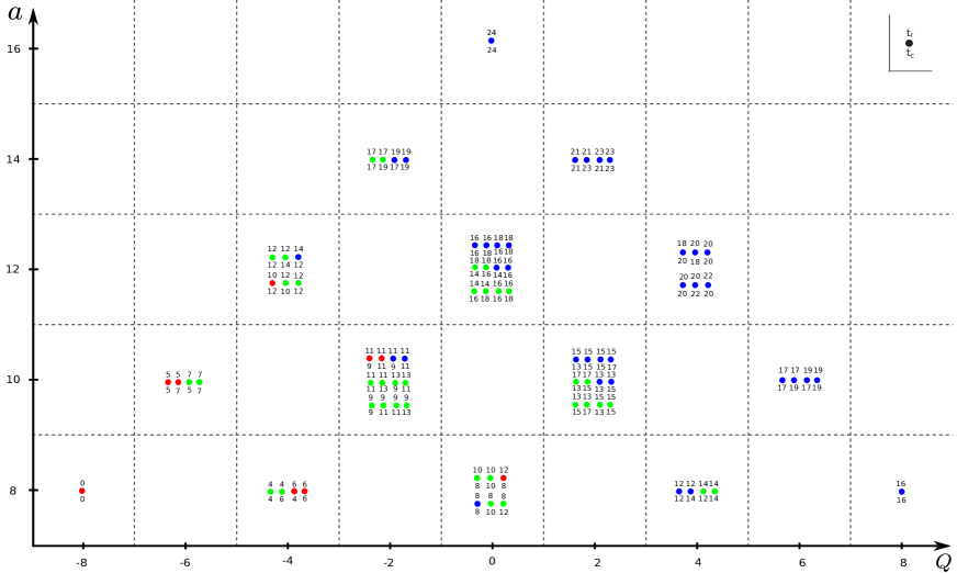
Figure 17: The $[2,2]$-colored HOMFLY homology of the figure-eight. The red dots represent the elements in $H_{*}(\widetilde{}\mathscr{H}^{\rm HOMFLY}_{[2,2]}({\bf 3_{1}}),d^{+}_{[2,2]\to[2]})$. The red, green and blue dots consist of the terms corresponding to $k=2,1$ and $0$ in the first summation of (264) respectively.

$$\widetilde{}\mathscr{P}_{\yng(2,2)}({\bf 3_{1}};a,Q,t_{r},t_{c})$$ (590)

$$={\color[rgb]{1,0,0}a^{8}\left(\tfrac{1}{Q^{8}}+\tfrac{t_{c}^{4}t_{r}^{6}}{Q^{4}}+\tfrac{t_{c}^{6}t_{r}^{6}}{Q^{4}}+t_{c}^{8}t_{r}^{12}\right)+a^{10}\left(\tfrac{t_{c}^{5}t_{r}^{5}}{Q^{6}}+\tfrac{t_{c}^{7}t_{r}^{5}}{Q^{6}}+\tfrac{t_{c}^{9}t_{r}^{11}}{Q^{2}}+\tfrac{t_{c}^{11}t_{r}^{11}}{Q^{2}}\right)+\tfrac{a^{12}t_{c}^{12}t_{r}^{10}}{Q^{4}}}$$ (591)

$${\color[rgb]{0.133,0.545,0.133}+a^{8}\left(\tfrac{t_{c}^{4}t_{r}^{4}}{Q^{4}}+\tfrac{t_{c}^{6}t_{r}^{4}}{Q^{4}}+t_{c}^{10}t_{r}^{8}+t_{c}^{12}t_{r}^{8}+t_{c}^{8}t_{r}^{10}+t_{c}^{10}t_{r}^{10}+Q^{4}t_{c}^{12}t_{r}^{14}+Q^{4}t_{c}^{14}t_{r}^{14}\right)}$$ (592)

$${\color[rgb]{0.133,0.545,0.133}+a^{10}\Big{(}\tfrac{t_{c}^{5}t_{r}^{7}}{Q^{6}}+\tfrac{t_{c}^{7}t_{r}^{7}}{Q^{6}}+\tfrac{t_{c}^{9}t_{r}^{9}}{Q^{2}}+\tfrac{2t_{c}^{11}t_{r}^{9}}{Q^{2}}+\tfrac{t_{c}^{13}t_{r}^{9}}{Q^{2}}+\tfrac{t_{c}^{11}t_{r}^{11}}{Q^{2}}+\tfrac{t_{c}^{13}t_{r}^{11}}{Q^{2}}+\tfrac{t_{c}^{9}t_{r}^{13}}{Q^{2}}+\tfrac{t_{c}^{11}t_{r}^{13}}{Q^{2}}}$$ (593)

$${\color[rgb]{0.133,0.545,0.133}\hskip 142.26378pt+Q^{2}t_{c}^{15}t_{r}^{13}+Q^{2}t_{c}^{17}t_{r}^{13}+Q^{2}t_{c}^{13}t_{r}^{15}+Q^{2}t_{c}^{15}t_{r}^{15}+Q^{2}t_{c}^{13}t_{r}^{17}+Q^{2}t_{c}^{15}t_{r}^{17}\Big{)}}$$ (594)

$${\color[rgb]{0.133,0.545,0.133}+a^{12}\left(\tfrac{t_{c}^{10}t_{r}^{12}}{Q^{4}}+\tfrac{2t_{c}^{12}t_{r}^{12}}{Q^{4}}+\tfrac{t_{c}^{14}t_{r}^{12}}{Q^{4}}+t_{c}^{16}t_{r}^{14}+t_{c}^{18}t_{r}^{14}+t_{c}^{16}t_{r}^{16}+t_{c}^{18}t_{r}^{16}+t_{c}^{14}t_{r}^{18}+t_{c}^{16}t_{r}^{18}\right)+a^{14}\left(\tfrac{t_{c}^{17}t_{r}^{17}}{Q^{2}}+\tfrac{t_{c}^{19}t_{r}^{17}}{Q^{2}}\right)}$$ (595)

$${\color[rgb]{0,0,1}+a^{8}\left(t_{c}^{8}t_{r}^{8}+Q^{4}t_{c}^{12}t_{r}^{12}+Q^{4}t_{c}^{14}t_{r}^{12}+Q^{8}t_{c}^{16}t_{r}^{16}\right)}$$ (596)

$${\color[rgb]{0,0,1}+a^{10}\Big{(}\tfrac{t_{c}^{9}t_{r}^{11}}{Q^{2}}+\tfrac{t_{c}^{11}t_{r}^{11}}{Q^{2}}+Q^{2}t_{c}^{13}t_{r}^{13}+Q^{2}t_{c}^{15}t_{r}^{13}+Q^{2}t_{c}^{13}t_{r}^{15}+2Q^{2}t_{c}^{15}t_{r}^{15}+Q^{2}t_{c}^{17}t_{r}^{15}}$$ (597)

$${\color[rgb]{0,0,1}\hskip 170.71652pt+Q^{6}t_{c}^{17}t_{r}^{17}+Q^{6}t_{c}^{19}t_{r}^{17}+Q^{6}t_{c}^{17}t_{r}^{19}+Q^{6}t_{c}^{19}t_{r}^{19}\Big{)}}$$ (598)

$${\color[rgb]{0,0,1}+a^{12}\left(\tfrac{t_{c}^{12}t_{r}^{14}}{Q^{4}}+t_{c}^{14}t_{r}^{16}+2t_{c}^{16}t_{r}^{16}+t_{c}^{18}t_{r}^{16}+t_{c}^{16}t_{r}^{18}+t_{c}^{18}t_{r}^{18}+Q^{4}t_{c}^{20}t_{r}^{18}+Q^{4}t_{c}^{18}t_{r}^{20}+2Q^{4}t_{c}^{20}t_{r}^{20}+Q^{4}t_{c}^{22}t_{r}^{20}+Q^{4}t_{c}^{20}t_{r}^{22}\right)}$$ (599)

$${\color[rgb]{0,0,1}+a^{14}\left(\tfrac{t_{c}^{17}t_{r}^{19}}{Q^{2}}+\tfrac{t_{c}^{19}t_{r}^{19}}{Q^{2}}+Q^{2}t_{c}^{21}t_{r}^{21}+Q^{2}t_{c}^{23}t_{r}^{21}+Q^{2}t_{c}^{21}t_{r}^{23}+Q^{2}t_{c}^{23}t_{r}^{23}\right)+a^{16}t_{c}^{24}t_{r}^{24}}$$ (600)

References

- (1) E. Witten, Quantum Field Theory and the Jones Polynomial, Commun. Math. Phys. 121 (1989) 351–399.
- (2) N. Y. Reshetikhin and V. G. Turaev, Ribbon graphs and their invaraints derived from quantum groups, Comm. Math. Phys. 127 (1990), no. 1 1–26.
- (3) V. Jones, A polynomial invariant for knots via von Neumann algebras, Bull. Am. Math. Soc. 12 (1985) 103–111.
- (4) M. Khovanov, A categorification of the Jones polynomial, Duke Math. J. 3 (2000) 359–426, [math/9908171].
- (5) B. Webster, Knot invariants and higher representation theory II: the categorification of quantum knot invariants, arXiv:1005.4559.
- (6) B. Cooper and V. Krushkal, Categorification of the Jones-Wenzl projectors, Quantum Topology 3 (2012) 139–180, [arXiv:1005.5117].
- (7) I. Frenkel, C. Stroppel, and J. Sussan, Categorifying fractional Euler characteristics, Jones-Wenzl projector and -symbols, Quantum Topology 3 (2012) 181–253, [arXiv:1007.4680].
- (8) M. Khovanov and L. Rozansky, Matrix factorizations and link homology, Fund. Math. 199 (2008) 1–91, [math/0401268].
- (9) M. Khovanov and L. Rozansky, Matrix factorizations and link homology II, Geom. Topol. 12 (2008), no. 3 1387–1425, [math/0505056].
- (10) P. Freyd, D. Yetter, J. Hoste, W. Lickorish, K. Millett, A. Ocneanu, and D. Yetter, A new polynomial invariant of knots and links, Bull. Am. Math. Soc. 12 (1985) 239–246.
- (11) J. H. Przytycki and P. Traczyk, Conway algebras and skein equivalence of links, Amer. Math. Soc. (1987) 744–748.
- (12) S. Gukov, A. S. Schwarz, and C. Vafa, Khovanov-Rozansky homology and topological strings, Lett.Math.Phys. 74 (2005) 53–74, [hep-th/0412243].
- (13) N. M. Dunfield, S. Gukov, and J. Rasmussen, The Superpolynomial for knot homologies, Experimental Mathematics 15 (2006), no. 2 129–159, [math/0505662].
- (14) S. Gukov and M. Stosic, Homological Algebra of Knots and BPS States, arXiv:1112.0030.
- (15) E. Gorsky, S. Gukov, and M. Stosic, Quadruply-graded colored homology of knots, arXiv:1304.3481.
- (16) L. H. Kauffman, On knots, vol. 115. Princeton university press, 1987.
- (17) S. Stevan, Chern-Simons Invariants of Torus Links, Annales Henri Poincare 11 (2010) 1201–1224, [arXiv:1003.2861].
- (18) S. Sinha and C. Vafa, SO and Sp Chern-Simons at large N, hep-th/0012136.
- (19) M. Marino, String theory and the Kauffman polynomial, Commun.Math.Phys. 298 (2010) 613–643, [arXiv:0904.1088].
- (20) S. Gukov and J. Walcher, Matrix factorizations and Kauffman homology, hep-th/0512298.
- (21) M. Aganagic and S. Shakirov, Knot Homology from Refined Chern-Simons Theory, arXiv:1105.5117.
- (22) P. Dunin-Barkowski, A. Mironov, A. Morozov, A. Sleptsov, and A. Smirnov, Superpolynomials for toric knots from evolution induced by cut-and-join operators, JHEP 03 (2013) 021, [arXiv:1106.4305].
- (23) H. Fuji, S. Gukov, P. Sulkowski, and H. Awata, Volume Conjecture: Refined and Categorified, Adv.Theor.Math.Phys. 16 (2012) 1669–1777, [arXiv:1203.2182].
- (24) E. Gorsky and A. Negut, Refined knot invariants and Hilbert schemes, arXiv:1304.3328.
- (25) I. Cherednik, Jones polynomials of torus knots via DAHA, arXiv:1111.6195.
- (26) M. Aganagic and K. Schaeffer, Orientifolds and the Refined Topological String, JHEP 1209 (2012) 084, [arXiv:1202.4456].
- (27) H. Fuji, S. Gukov, and P. Sulkowski, Super-A-polynomial for knots and BPS states, Nucl.Phys. B867 (2013) 506–546, [arXiv:1205.1515].
- (28) H. Fuji, S. Gukov, M. Stosic, and P. Sulkowski, 3d analogs of Argyres-Douglas theories and knot homologies, JHEP 1301 (2013) 175, [arXiv:1209.1416].
- (29) S. Nawata, P. Ramadevi, Zodinmawia, and X. Sun, Super-A-polynomials for Twist Knots, JHEP 1211 (2012) 157, [arXiv:1209.1409].
- (30) R. Kaul and T. Govindarajan, Three-dimensional Chern-Simons theory as a theory of knots and links, Nucl.Phys. B380 (1992) 293–336, [hep-th/9111063].
- (31) R. Kaul and T. Govindarajan, Three-dimensional Chern-Simons theory as a theory of knots and links. 2. Multicolored links, Nucl.Phys. B393 (1993) 392–412.
- (32) P. Rama Devi, T. Govindarajan, and R. Kaul, Three-dimensional Chern-Simons theory as a theory of knots and links. 3. Compact semisimple group, Nucl.Phys. B402 (1993) 548–566, [hep-th/9212110].
- (33) R. Kaul, Chern-Simons theory, colored oriented braids and link invariants, Commun.Math.Phys. 162 (1994) 289–320, [hep-th/9305032].
- (34) K. Yamagishi, M.-L. Ge, and Y.-S. Wu, New hierarchies of knot polynomials from topological Chern-Simons gauge theory, Lett. Math. Phys. 19 (1990) 15.
- (35) K. Yamagishi and Y.-S. Wu, Chern-Simons Theory and Kaufman Polynomials, Int.J.Mod.Phys. A 05 (1990), no. 06 1165–1195.
- (36) J. H. Horne, Skein relations and Wilson loops in Chern-Simons gauge theory, Nucl. Phys. B334 (1990) 669–694.
- (37) M. Rosso and V. Jones, On the invariants of torus knots derived from quantum groups, J.Knot Theor.Ramifications 2 (1993) 97.
- (38) J. Labastida, P. Llatas, and A. Ramallo, Knot operators in Chern-Simons gauge theory, Nucl.Phys. B348 (1991) 651–692.
- (39) X.-S. Lin and H. Zheng, On the hecke algebras and the colored homfly polynomial, Trans. Amer. Math. Soc 362 (2010) 1–18.
- (40) A. Brini, B. Eynard, and M. Marino, Torus knots and mirror symmetry, Annales Henri Poincare 13 (2012) 1873–1910, [arXiv:1105.2012].
- (41) J. Labastida and E. Perez, A Relation between the Kauffman and the HOMFLY polynomials for torus knots, q-alg/9507031.
- (42) E. Witten, Chern-Simons gauge theory as a string theory, Prog. Math. 133 (1995) 637–678, [hep-th/9207094].
- (43) R. Gopakumar and C. Vafa, On the gauge theory/geometry correspondence, Adv. Theor. Math. Phys. 3 (1999) 1415–1443, [hep-th/9811131].
- (44) H. Ooguri and C. Vafa, Knot invariants and topological strings, Nucl.Phys. B577 (2000) 419–438, [hep-th/9912123].
- (45) V. Bouchard, B. Florea, and M. Marino, Counting higher genus curves with crosscaps in Calabi-Yau orientifolds, JHEP 0412 (2004) 035, [hep-th/0405083].
- (46) V. Bouchard, B. Florea, and M. Marino, Topological open string amplitudes on orientifolds, JHEP 0502 (2005) 002, [hep-th/0411227].
- (47) P. Borhade and P. Ramadevi, SO(N) reformulated link invariants from topological strings, Nucl.Phys. B727 (2005) 471–498, [hep-th/0505008].
- (48) R. Gopakumar and C. Vafa, M-theory and topological strings. I, hep-th/9809187.
- (49) R. Gopakumar and C. Vafa, M-theory and topological strings. II, hep-th/9812127.
- (50) J. Labastida, M. Marino, and C. Vafa, Knots, links and branes at large N, JHEP 0011 (2000) 007, [hep-th/0010102].
- (51) E. Witten, Fivebranes and Knots, arXiv:1101.3216.
- (52) K. Hori, A. Iqbal, and C. Vafa, D-branes and mirror symmetry, hep-th/0005247.
- (53) M. Aganagic and C. Vafa, Mirror symmetry, D-branes and counting holomorphic discs, hep-th/0012041.
- (54) M. Aganagic, A. Klemm, and C. Vafa, Disk instantons, mirror symmetry and the duality web, Z.Naturforsch. A57 (2002) 1–28, [hep-th/0105045].
- (55) B. S. Acharya, M. Aganagic, K. Hori, and C. Vafa, Orientifolds, mirror symmetry and superpotentials, hep-th/0202208.
- (56) M. Aganagic and C. Vafa, Large N Duality, Mirror Symmetry, and a Q-deformed A-polynomial for Knots, arXiv:1204.4709.
- (57) A. Strominger, S.-T. Yau, and E. Zaslow, Mirror symmetry is T duality, Nucl.Phys. B479 (1996) 243–259, [hep-th/9606040].
- (58) B. Eynard and N. Orantin, Invariants of algebraic curves and topological expansion, Commun.Num.Theor.Phys. 1 (2007) 347–452, [math-ph/0702045].
- (59) R. Dijkgraaf, H. Fuji, and M. Manabe, The Volume Conjecture, Perturbative Knot Invariants, and Recursion Relations for Topological Strings, Nucl.Phys. B849 (2011) 166–211, [arXiv:1010.4542].
- (60) G. Borot and B. Eynard, All-order asymptotics of hyperbolic knot invariants from non-perturbative topological recursion of A-polynomials, arXiv:1205.2261.
- (61) J. A. Rasmussen, Some differentials on Khovanov-Rozansky homology, math/0607544.
- (62) A. Morozov, Special colored Superpolynomials and their representation-dependence, JHEP 1212 (2012) 116, [arXiv:1208.3544].
- (63) J. A. Rasmussen, Khovanov homology and the slice genus, Invent. Math. 182 (2010), no. 2 419 447, [math/0402131].
- (64) M. Khovanov and L. Rozansky, Virtual crossings, convolutions and a categorification of the Kauffman polynomial, math/0701333.
- (65) S. Shakirov, Colored knot amplitudes and Hall-Littlewood polynomials, arXiv:1308.3838.
- (66) A. Anokhina and A. Morozov, Cabling procedure for the colored HOMFLY polynomials, arXiv:1307.2216.
- (67) H. Murakami, An introduction to the volume conjecture and its generalizations, arXiv:0802.0039.
- (68) R. Kashaev, The Hyperbolic volume of knots from quantum dilogarithm, Lett.Math.Phys. 39 (1997) 269–275.
- (69) H. Murakami and J. Murakami, The colored Jones polynomials and the simplicial volume of a knot, ACTA MATHEMATICA 186 (2001), no. 1 85–104, [math/9905075].
- (70) S. Gukov, Three-dimensional quantum gravity, Chern-Simons theory, and the A polynomial, Commun.Math.Phys. 255 (2005) 577–627, [hep-th/0306165].
- (71) S. Gukov and H. Murakami, SL(2,C) Chern-Simons theory and the asymptotic behavior of the colored Jones polynomial, Lett.Math.Phys. 86 (2008) 79–98, [math/0608324].
- (72) E. Witten, Analytic Continuation Of Chern-Simons Theory, arXiv:1001.2933.
- (73) D. Cooper, M. Culler, H. Gillet, D. Long, and P. Shalen, Plane curves associated to character varieties of 3-manifolds, Invent. Math. 118 (1994) 47–84. http://www.math.ucsb.edu/~long/pubpdf/CCGLS.pdf.
- (74) T. Dimofte and S. Gukov, Chern-Simons Theory and S-duality, JHEP 1305 (2013) 109, [arXiv:1106.4550].
- (75) S. Garoufalidis, On the characteristic and deformation varieties of a knot, Geometry Topology Monographs. 7 (2004) 291–309, [math/0306230].
- (76) S. Garoufalidis and T. Le, The colored Jones function is holonomic, Geometry Topology. 9 (2004) 1253–1293, [math/0309214].
- (77) S. Garoufalidis, The colored HOMFLY polynomial is q-holonomic, arXiv:1211.6388.
- (78) S. Gukov and P. Sulkowski, A-polynomial, B-model, and Quantization, JHEP 1202 (2012) 070, [arXiv:1108.0002].
- (79) A. Champanerkar, A-polynomial and Bloch invariants of hyperbolic 3-manifolds, . Doctoral dissertation, Columbia University.
- (80) T. Dimofte, S. Gukov, and L. Hollands, Vortex Counting and Lagrangian 3-manifolds, Lett.Math.Phys. 98 (2011) 225–287, [arXiv:1006.0977].
- (81) Y. Terashima and M. Yamazaki, SL(2,R) Chern-Simons, Liouville, and Gauge Theory on Duality Walls, JHEP 1108 (2011) 135, [arXiv:1103.5748].
- (82) T. Dimofte, D. Gaiotto, and S. Gukov, Gauge Theories Labelled by Three-Manifolds, arXiv:1108.4389.
- (83) T. Dimofte, D. Gaiotto, and S. Gukov, 3-Manifolds and 3d Indices, arXiv:1112.5179.
- (84) J. Yagi, 3d TQFT from 6d SCFT, JHEP 1308 (2013) 017, [arXiv:1305.0291].
- (85) S. Lee and M. Yamazaki, 3d Chern-Simons Theory from M5-branes, arXiv:1305.2429.
- (86) C. Cordova and D. L. Jafferis, Complex Chern-Simons from M5-branes on the Squashed Three-Sphere, arXiv:1305.2891.
- (87) C. Beem, T. Dimofte, and S. Pasquetti, Holomorphic Blocks in Three Dimensions, arXiv:1211.1986.
- (88) T. Dimofte, D. Gaiotto, and R. van der Veen, RG Domain Walls and Hybrid Triangulations, arXiv:1304.6721.
- (89) H.-J. Chung, T. Dimofte, S. Gukov, and P. Sulkowski, 3d/3d correspondence revised, work in progress, .
- (90) L. Ng, Combinatorial knot contact homology and transverse knots, Advances in Mathematics. 277 (2011), no. 6 2189–2219, [arXiv:1010.0451].
- (91) T. Ekholm, J. Etnyre, L. Ng, and M. Sullivan, Filtrations on the knot contact homology of transverse knots, Mathematische Annalen (2013) 1–31, [arXiv:1010.0450].
- (92) S. Nawata, P. Ramadevi, and Zodinmawia, Multiplicity-free quantum -symbols for , arXiv:1302.5143.
- (93) K. Liu and P. Peng, Proof of the Labastida-Marino-Ooguri-Vafa conjecture, J. Diff. Geom. 85 (2010), no. 3 479–525, [arXiv:0704.1526].
- (94) K. Liu and P. Peng, On a proof of the Labastida-Marino-Ooguri-Vafa conjecture, Math.Res.Lett. 17 (2010) 493–506, [arXiv:1012.2635].
- (95) R. Hadji and H. Morton, A basis for the full Homfly skein of the annulus, Math. Proc. Cambridge Philos. Soc. 141 (2006) 81–100, [math/0408078].
- (96) C. Paul, P. Borhade, and P. Ramadevi, Composite Invariants and Unoriented Topological String Amplitudes, arXiv:1003.5282.