Two-setting multi-site Bell inequalities for loophole-free tests with up to 50% loss

Abstract

We consider Bell experiments with $N$ spatially separated qubits where loss is present and restrict to two measurement settings per site. We note the Mermin-Ardehali-Belinskii-Klyshko (MABK) Bell inequalities do not present a tight bound for the predictions of local hidden variable (LHV) theories. The Holder-type Bell inequality derived by Cavalcanti, Foster, Reid and Drummond provides a tighter bound, for high losses. We analyse the actual tight bound for the MABK inequalities, given the measure $W=\prod_{k=1}^{N}\eta_{k}$ of overall detection efficiency, where $\eta_{k}$ is the efficiency at the site $k$. Using these inequalities, we confirm that the maximally entangled Greenberger-Horne-Zeilinger state enables loophole-free falsification of LHV theories provided $\prod_{k=1}^{N}\eta_{k}>2^{(2-N)}$, which implies a symmetric threshold efficiency of $\eta\rightarrow 50\%$ , as $N\rightarrow\infty$. Furthermore, loophole-free violations remain possible, even when the efficiency at some sites is reduced well below $0.5$, provided $N>3$.

I Introduction

Bell showed the inconsistency of local realism with quantum mechanics, by deriving a constraint on the correlations predicted by any local hidden variable (LHV) theory bell . For some quantum states, these constraints, called Bell inequalities, are violated. Bell’s discovery of quantum nonlocality has inspired countless investigations cs ; clexp ; aspect ; weihs and, through the close connection with entanglement entperes , underpins the field of quantum information.

A major challenge is to understand the interplay of Bell’s nonlocality with loss, which is defined by the ratio, $\eta$, of the number of detected to emitted particles. Loss caused by detector inefficiencies has resulted in the famous “detection loophole” for testing Bell’s correlations in the laboratory loopholdet . To date, there has been no loophole-free violation of a Bell inequality for spacelike separated measurement events. Furthermore, the sensitivity of loophole-free Bell nonlocality to transmission losses is intimately related to the security of quantum cryptography cry . Motivated by all this, there has been a considerable effort to work out the smallest value of $\eta$ required for a loophole-free violation of a Bell inequality.

Bell’s original gedanken experiment involved measurement of the spin correlations of two maximally entangled and spatially separated spin-$1/2$ particles. His inequality, and the equally famous version derived by Clauser-Horne-Shimony-Holt (CHSH), required only two measurement settings, for each particle bell ; bell2 ; chsh . Despite the importance of this inequality and its $N$-particle generalisations, the Mermin-Ardehali-Belinski-Klyshko (MABK) inequalities mermin-1 ; ardehali ; bk , surprisingly little is known about how to achieve a violation of them, for reduced efficiencies, $\eta$.

Where there are only two spatially separated particles ($N=2$), Garg and Mermin put forward a modified CHSH inequality that could be violated for $\eta>0.83$ gargmer . Their inequality removed the necessity of heralding the emission events, since the inequality did not specify the total number of undetected particle pairs. Eberhard showed that the Clauser-Horne (CH) inequality CH would yield violations for as low as $\eta>0.67$ using non-maximally entangled states, also without the need for heralding ebernonmaxch . Where measurements are made on $N$ spin-$1/2$ systems, at each of $N$ sites, Larsson and Semitecolos (LS) proved that for CH-type inequalities, $\eta>\frac{N}{2N-1}$ was sufficient, at least for some quantum state. They concluded “there are $N$- site experiments for which the quantum mechanical predictions violate local realism whenever $\eta>0.5$” LS . Despite this knowledge, it remained unclear how to demonstrate this nonlocality, as no specific inequality and state was proposed that would enable realisation of Bell’s nonlocality for efficiencies $\eta$ as low as $0.5$ for each detector.

An explicit loophole-free demonstration of Bell nonlocality using the MABK inequalities and the maximally entangled Greenberger-Horne-Zeilinger (GHZ) states ghz was shown possible, with heralding, for $\eta>2^{(1-N)/2N}$ braunmann . However, the lowest threshold here requires $\eta>0.71$. Cabello, Rodriguez and Villanueva (CRV) established that the LS limit is achievable, for large $N$ and for the GHZ states, by proving that $\eta>\frac{N}{2N-2}$ was necessary and sufficient for Bell nonlocality in the case of $N$ odd. However, no inequality was proposed cabello-1 . Firm proposals have been given however for efficiencies as low as $\eta\rightarrow 0.5$ at one detector, but only for non-maximally entangled states and provided an atom could be detected with 100% efficiency at a second site cablarasy ; asymmbrunner .

In this paper, we contribute further to these results, by constructing a tighter version of the MABK inequalities. Insight is gained from the recent work of Cavalcanti et al and Acin et al cvbell2-1-1 ; vogelshc ; acincavalcfrd ; cvbell ; prlholdcfrd ; cfrdwig ; cavalpranonlocality who derived a “Holder” Bell inequality that allows realisation of the LS-CRV efficiency threshold of near $50\%$ for high $N$. We will see that the tight MABK inequality is in fact a melding of the new Holder inequality (which dominates at lower efficiencies) and the old MABK inequality (which dominates at high efficiencies).

In this way, we show it possible to violate a two-setting Bell inequality loophole-free, using a maximally entangled GHZ state, whenever $\prod_{k=1}^{N}\eta_{k}>2^{(2-N)}$, for $N\geq 3$. Here, $\eta_{k}$ is the efficiency at site $k$. For symmetric sites, the threshold efficiency reduces to $\eta\rightarrow 0.5$ as $N\rightarrow\infty$, as given in Ref. cavalpranonlocality . In fact, as we confirm in this paper, $\eta\rightarrow 0.5$ is the best result possible, since we reason that $\eta>1/m$ is required to demonstrate Bell’s nonlocality using $m$-setting inequalities. Furthermore, we establish that where $N>3$, the loophole-free violation of the two-setting Bell inequality does not require $\eta_{k}>0.5$ for each site $k$, but can be achieved even if the efficiencies are very low at some sites.

We conclude with a brief discussion, pointing out that three or more sites are required if one is to obtain the violations of the two-setting inequalities in the lossy scenarios. We then conjecture whether these violations can signify a genuine multi-partite Bell nonlocality, in the sense defined by Svetlichny and Collins et al svet .

II Holder Bell inequalities

Let us begin by presenting the Bell inequalities derived by Cavalcanti, Foster, Reid and Drummond (CFRD) cvbell2-1-1 . We define a set of space-like separated measurements $\hat{X_{\theta_{k}}^{k}}$ that can be performed on each of $k$ systems ($k=1,...,N$). We consider only two settings, $\theta_{1}$ and $\theta_{2}$, at each site, and so denote $\hat{X_{\theta_{1}}^{k}}=\hat{A_{k}}$ and $\hat{X_{\theta_{2}}^{k}}=\hat{B_{k}}$. For any LHV theory, it is true that cvbell2-1-1 ; vogelshc ; cvbell

$$\Bigl{|}\Bigl{\langle}\prod_{k=1}^{N}(A_{k}+iB_{k})\Bigr{\rangle}\Bigr{|}^{2} \leq \Bigl{\langle}\prod_{k=1}^{N}\{(A_{k})^{2}+(B_{k})^{2}\}\Bigr{\rangle},$$ (1)

where $A_{k}$, $B_{k}$ are the outcomes for the measurements $\hat{A_{k}}$ and $\hat{B_{k}}$ respectively. The left side of the inequality is written in a compact form and involves moments of the Hermitian observables $\hat{A_{k}}$ and $\hat{B_{k}}$ defined at each site. Violation of this inequality will imply failure of LHV theories, and hence Bell’s nonlocality.

The inequality (1) and its variants are closely associated with the Holder inequalities used in mathematical analysis holder . For this reason, the inequalities based on (1) will be referred to throughout this paper as the “Holder Bell inequalities”. The best known mathematical Holder inequality is the Cauchy Schwarz inequality. The distinctive feature for our purposes is that the upper bound given by the right-side of a Holder inequality is moment-dependent. This will give an advantage for detecting Bell’s nonlocality in lossy scenarios.

The authors of Refs. acincavalcfrd ; cavalpranonlocality have derived the application of the inequality (1) to the scenario of $N$ spin-$1/2$ systems, as in the original Bell and GHZ gedanken experiments bell ; ghz . Here, one assigns $\hat{X_{\theta}^{k}}=\hat{\sigma_{k}}^{\theta}=\hat{\sigma_{k}}^{x}\cos\theta+\hat{\sigma_{k}}^{y}\sin\theta$, where $\hat{\sigma_{k}}^{x/y}$ are the Pauli spin operators for site $k$, and $\theta$ can be different for each site. Since the outcomes of the measurement are always $+1$ or $-1$, the inequality (1) will reduce to acincavalcfrd ; cavalpranonlocality

$$\Bigl{|}\Bigl{\langle}\prod_{k=1}^{N}(A_{k}+iB_{k})\Bigr{\rangle}\Bigr{|} \leq 2^{N/2}.\,$$ (2)

When the combination of moments given by the left side of the inequality exceeds $2^{N/2}$, one can claim failure of LHV models.

Supposing there is inefficient detection, we follow Bell’s analysis bell2 ; cs ; gargmer and note that for each emission event, the “spin” measurement made on each particle will have three possible outcomes, depending on whether the spin is measured “up”, “down”, or if there is “no detection”. The three outcomes are assigned the numerical result $+1$, $-1$ and $0$, respectively. That is, each $A_{k}$ and $B_{k}$ can now have values $\pm 1$ or $0$. Then, we note that the inequality deduced from (1) changes. While the inequality (2) is still valid, it is too restrictive. The moments of the right-side are no longer necessarily given by $2^{N/2}$ as in the perfect efficiency case of (2), but can be measured, and compared with those of the left-side, to give a more sensitive test for failure of LHV theories.

In practice, assuming a detection efficiency $\eta_{k}$ for both measurements ($A_{k}$ and $B_{k}$) at site $k$, the right-side of the inequality (2) is predicted to be $2^{N/2}(\eta_{1}\eta_{2}...\eta_{N})^{1/2}$. The inequality reduces to

$$\Bigl{|}\Bigl{\langle}\prod_{k=1}^{N}(A_{k}+iB_{k})\Bigr{\rangle}\Bigr{|} \leq 2^{N/2}(\eta_{1}\eta_{2}...\eta_{N})^{1/2}\,.$$ (3)

This gives us the desired result, that the Bell inequality has a LHV bound (given by the right-side) that reduces with efficiency $\eta_{k}$.

Next, we establish the connection with the well-known MABK Bell inequalities, by noting there are two different forms of the Holder Bell inequalities (1) and (3). If $x^{2}+y^{2}=r^{2}$, then it is always true that $x+y\leq\sqrt{2}r$, where $x,\,y,\,r$ are real numbers. Thus, on separating $\langle\prod_{k=1}^{N}(A_{k}+iB_{k})\rangle$ into real and imaginary parts (denoted by symbols $\Re e$ and $\Im m$), the Holder Bell inequality (1) implies the Bell inequality

$$Ar_{N} \equiv s_{R}\Re e\Bigl{\langle}\prod_{k=1}^{N}(A_{k}+iB_{k})\Bigr{\rangle}+s_{I}\Im m\Bigl{\langle}\prod_{k=1}^{N}(A_{k}+iB_{k})\Bigr{\rangle}$$ (4)

$$\leq\sqrt{2}\Bigl{\langle}\prod_{k=1}^{N}\{A_{k}^{2}+B_{k}^{2}\}\Bigr{\rangle}^{1/2}$$

(where $s_{R},s_{I}=\pm 1$). Using the reasoning explained above, this inequality reduces to

$$Ar_{N}\leq 2^{(N+1)/2}(\eta_{1}\eta_{2}...\eta_{N})^{1/2}$$ (5)

for the lossy experiment, which gives a useful version of the inequality (3). The inequalities (4) and (5) have the same left-side as the subset of MABK inequalities called the Ardehali inequalities ardehali , and we have therefore denoted the left-side by the symbol $Ar_{N}$.

Also, following directly from (1), because for any complex number $z=\Re ez+i\Im mz$ it is true that $\Re ez,\Im mz\leq|z|$, it follows that for any LHV model

$$M_{N} \leq \Bigl{\langle}\prod_{k=1}^{N}\{A_{k}^{2}+B_{k}^{2}\}\Bigr{\rangle}^{1/2}$$ (6)

where we can select $M_{N}$ to be either of $\Re e\langle\prod_{k=1}^{N}(A_{k}+iB_{k})\rangle$ or $\Im m\langle\prod_{k=1}^{N}(A_{k}+iB_{k})\rangle$. In the presence of losses, the inequality (6) becomes

$$M_{N}\leq 2^{N/2}(\eta_{1}\eta_{2}...\eta_{N})^{1/2}$$ (7)

which gives a second useful version of the inequality (3). In this case, the inequalities have the same left-side as the subset of MABK inequalities derived by Mermin mermin-1 , and we have therefore denoted the left-side by the symbol $M_{N}$.

The Bell inequalities (4) and (6) were derived, from a different perspective, by Cavalcanti et al cavalpranonlocality . We will show below that while the two Holder Bell inequalities given by (4) and (6) have the same left-side as the MABK Bell inequalities, the right-side is different.

III MABK Bell inequalities

The left-side of the Holder Bell inequalities (4) and (6) corresponds precisely to that used in the well known Bell inequalities of MABK mermin-1 ; ardehali ; bk . We now present the MABK Bell inequalities. In the MABK case, a different bound is obtained for the LHV prediction. When $\eta_{k}=1$, this bound is clearly tighter than that derived for the Holder inequalities.

The MABK inequalities consist of two subsets, one for even $N$ and one for odd $N$. The well-known “Ardehali” MABK Bell inequality applies only to even $N$, and is ardehali

$$Ar_{N} \leq 2^{N/2}.$$ (8)

When $N=2$, the left side becomes

$$S=Ar_{2}=\langle A_{1}A_{2}\rangle-\langle B_{1}B_{2}\rangle+\langle A_{1}B_{2}\rangle+\langle B_{1}A_{2}\rangle$$ (9)

and Ardehali’s inequality reduces to the well-known CHSH inequality, $S\leq 2$. For the case of $N$ odd, only, Mermin proved the Bell inequality mermin-1

$$M_{N} \leq 2^{(N-1)/2}\,.$$ (10)

Combined, the two inequalities (8) and (10) give a LHV prediction for arbitrary $N$, and are commonly termed the “MABK inequalities” mermin-1 ; ardehali ; bk .

The Ardehali and Mermin Bell inequalities are also valid for the lossy scenario, where “no detection” outcomes are assigned the outcome “$0$” bell2 ; braunmann . However, we can see immediately on comparison with the Holder Bell inequalities (5) and (7) that, for the lossy experiment, the MABK inequalities can no longer be tight. A similar result is known for these inequalities even in the context of pure states: MABK inequalities do not detect the Bell nonlocality that has been shown to exist for nonmaximally entangled generalised GHZ states mabknottight .

IV Quantum predictions

Now, we examine the predictions given by the maximally entangled GHZ state $\frac{1}{\sqrt{2}}\{|\uparrow\rangle^{\otimes N}-|\downarrow\rangle^{\otimes N}\}$, where $|\uparrow\rangle_{k}$, $|\downarrow\rangle_{k}$ are the eigenstates of the Pauli spin observable $\hat{\sigma}_{k}^{z}$, and $|\uparrow\rangle^{\otimes N}\equiv\prod_{k=1}^{N}|\uparrow\rangle_{k}$ wernerwolfmaxghz-2 . Mermin showed that if we choose measurement settings to correspond to either $\hat{\sigma}_{k}^{x}$ or $\hat{\sigma}_{k}^{y}$ for each $j=1,...,N$, then for optimally chosen settings, the quantum prediction is $M_{N}=2^{N-1}$, for $N$ odd mermin-1 . For the Ardehali’s inequalities, the optimal measurement choice involves a $\hat{\sigma}_{k}^{x}$ or $\hat{\sigma}_{k}^{y}$ setting for $N-1$ sites, with a rotated setting for the $N$th site ardehali . Then, the optimal quantum prediction is $Ar_{N}=2^{N-1/2}$, for $N$ even. Assuming symmetric detector efficiencies $\eta_{k}=\eta$, the optimal quantum prediction in the lossy case will be $S=\eta^{2}2\sqrt{2}$, $M_{N}=\eta^{N}2^{N-1}$ (for odd $N$), and $Ar_{N}=\eta^{N}2^{N-1/2}$ (for $N$even). Using the MABK Bell inequalities directly, this gives the efficiency threshold $\eta>2^{(1-N)/2N}$ for all $N$, which reduces to a lowest value of $\eta\rightarrow 0.71$ as $N\rightarrow\infty$, as shown by Braunstein and Mann braunmann .

As pointed out in Ref. cavalpranonlocality , the Holder Bell inequalities (4) and (6) will give a lower efficiency threshold in the symmetric case, for all $N>3$. If we consider odd $N$, then we use the inequality (6), for which the right-side is predicted to be $2^{N/2}\eta^{N/2}$ (corresponding to Eq. (7)). For even $N$, we use the inequality (4) for which the right-side is $2^{(N+1)/2}\eta^{N/2}$ (corresponding to Eq. (5)). The associated threshold efficiency for violation of the Holder-Bell inequalities is given by $\eta>2^{(-1+2/N)}$ for all $N\geq 3$ cavalpranonlocality . This threshold reduces to $0.79$ for $N=3$, and approaches $0.5$ as $N\rightarrow\infty$.

V LHV theory predictions

Having confirmed that neither the MABK nor the Holder Bell inequalities can provide the tight LHV bound in the presence of loss (poor detection efficiencies), our objective is to gain insight into the actual LHV predictions, and to then determine if lower efficiency thresholds are possible for a given $N$.

For all LHV theories, it is true that bell

$$E(X_{\theta_{1}}^{1},...,X_{\theta_{N}}^{N})=\int_{\lambda}p(\lambda)E_{\lambda}(X_{\theta_{1}}^{1})...E_{\lambda}(X_{\theta_{n}}^{N})d\lambda\,$$ (11)

where $E(X_{\theta_{1}}^{1},...,X_{\theta_{N}}^{N})$ is the expectation value for the product of outcomes $X_{\theta_{k}}^{k}$ of simultaneous measurements $\hat{X_{\theta_{k}}^{k}}$ ($k=1,...,N$) performed on the $N$ spatially separated systems. Here, $\{\lambda\}$ symbolises the set of local hidden variables of the LHV theory. Thus, $E_{\lambda}(X_{\theta_{k}}^{k})$ is the expectation value of $X_{\theta_{k}}^{k}$ given the hidden variable specification $\{\lambda\}$, and $p(\lambda)$ is the underlying probability distribution for $\{\lambda\}$.

We consider the LHV prediction for the terms $S$, $M_{N}$, $Ar_{N}$ of the CHSH, Mermin and Ardehali inequalities. We also introduce $W_{N}$ as a measure of overall efficiency. Specifically:

$$W_{N} = \frac{1}{2^{N}}\langle\prod_{k=1}^{N}\{|A_{k}|+|B_{k}|\}\rangle$$ (12)

Where the outcomes of $A_{k}$ and $B_{k}$ are given by $+1$, $-1$ or $0$, it is clear that $W_{N}=\frac{1}{2^{N}}R$, where $R$ is the right side of the Holder inequalities (4) and (6). In fact, there are $2^{N}$ relevant efficiencies $\eta$, one for each measurement setting ($A_{k}$ or $B_{k}$) at each site $k$. Where the efficiencies are equal for the two settings, and given at site $k$ by $\eta_{k}$, the quantum prediction for (12) is $W_{N}=\prod_{k=1}^{N}\eta_{k}$. A complication is that to measure the actual values of $S$, $M_{N}$, $Ar_{N}$ and $W_{N}$, it is necessary to establish all emission events, using an “event ready” or “heralding” apparatus bell2 ; cs . This is a significant but not insurmountable challenge herald .

It is possible to show that for any LHV model bell2 ; cs

$$\langle S\rangle=\int_{\lambda}p(\lambda)S_{\lambda}d\lambda,\,\,\,\,\,\,\,\,\langle W_{N}\rangle=\int_{\lambda}p(\lambda)W_{N,\lambda}d\lambda.$$ (13)

Similar expressions exist for $\langle M_{N}\rangle$ and $\langle Ar_{N}\rangle$. Here, $S_{\lambda}=\langle A_{1}\rangle_{\lambda}\langle A_{2}\rangle_{\lambda}-\langle A_{1}\rangle_{\lambda}\langle B_{2}\rangle_{\lambda}+\langle B_{1}\rangle_{\lambda}\langle A_{2}\rangle_{\lambda}+\langle B_{1}\rangle_{\lambda}\langle B_{2}\rangle_{\lambda}$ and $W_{2,\lambda}=\langle|A_{1}|\rangle_{\lambda}\langle|A_{2}|\rangle_{\lambda}+\langle|A_{1}|\rangle_{\lambda}\langle|B_{2}|\rangle_{\lambda}+\langle|B_{1}|\rangle_{\lambda}\langle|A_{2}|\rangle_{\lambda}+\langle|B_{1}|\rangle_{\lambda}\langle|B_{2}|\rangle_{\lambda}$, where $\langle A_{k}\rangle_{\lambda}$, $\langle B_{k}\rangle_{\lambda}$ are the expectation values for $A_{k}$, $B_{k}$, given the hidden variable specification $\{\lambda\}$. Similar expansions can be given for $W_{N,\lambda}$, $M_{N,\lambda}$ and $Ar_{N,\lambda}$. We find that for any LHV theory, constraints exist for the possible values of $\langle S\rangle$, $\langle M_{N}\rangle$ and $\langle Ar_{N}\rangle$, given the value of $\langle W_{N}\rangle$. In other words, for any given experimentally measured value of $W_{N}$, there will be a constraint on the LHV predictions for $\langle S\rangle$, $\langle M_{N}\rangle$ and $\langle Ar_{N}\rangle$.

We determine these constraints as follows. The outcome $A_{k}$ is constrained to be one of $\pm 1$ or $0$. Thus, in the LHV model, it must be true that $-1\leq\langle A_{k}\rangle_{\lambda}\leq 1$. The LHV model will specify probabilities for the $+1$ and $-1$ outcome for $A_{k}$, for a given hidden variable specification $\{\lambda\}$. We denote these probabilities by $P_{\lambda}^{A}(+)$ and $P_{\lambda}^{A}(-)$. Then we see that $\langle A_{k}\rangle_{\lambda}=P_{\lambda}^{A}(+)-P_{\lambda}^{A}(-)$ whereas $\langle|A_{k}|\rangle_{\lambda}=P_{\lambda}^{A}(+)+P_{\lambda}^{A}(-)$. We note $P_{\lambda}^{A}(+)+P_{\lambda}^{A}(-)$ is in fact the efficiency value predicted for the measurement setting $A_{k}$, given the hidden variable specification $\{\lambda\}$, and we introduce the notation $\langle\eta_{k}^{A}\rangle_{\lambda}\equiv\langle|A_{k}|\rangle_{\lambda}=P_{\lambda}^{A}(+)+P_{\lambda}^{A}(-)$. Thus, for a given $\langle|A_{k}|\rangle_{\lambda}$, it follows that

$$-\langle\eta_{k}^{A}\rangle_{\lambda}\leq\langle A_{k}\rangle\leq\langle\eta_{k}^{A}\rangle_{\lambda}$$ (14)

and similarly

$$-\langle\eta_{k}^{B}\rangle_{\lambda}\leq\langle B_{k}\rangle\leq\langle\eta_{k}^{B}\rangle_{\lambda}.$$ (15)

We evaluate for each possible $\langle\eta_{k}^{A}\rangle_{\lambda}$, $\langle\eta_{k}^{B}\rangle_{\lambda}$, the possible values of $S_{\lambda}$ and $W_{\lambda}$, which is a simple numeric exercise. For a given $W_{\lambda}$, the possible values of $S_{\lambda}$ can be displayed as a scattering of points on a diagram. We can then sample again over all possible distributions $p(\lambda)$ to evaluate the consistent predictions for both $W_{2}$ and $S$, for any possible LHV theory distribution. The same procedure is performed, to evaluate the possible $M_{N}$ and $A_{N}$, for a given $W_{N}$.

In fact, the full sampling is a tedious task. For our purposes, because we have two analytical bounds on the LHV predictions, we sample LHV predictions only to verify the bounds, and to establish the degree of tightness of them. Our sampling involves evaluating the possible $S$, $Ar_{N}$ or $M_{N}$, and $W_{N}$ when hidden variables assume the extreme values of $\pm 1$, or the value $0$, which in the absence of loss would amount to assuming a deterministic LHV theory fine . This does not cover all stochastic LHV theories, but we will see is enough to establish the validity and degree of tightness of the analytical MABK and Holder limits, for a given $W_{N}$.

VI Tightness of the inequalities

Before analysing the results, we give a geometrical interpretation of the degree of tightness of the Holder and MABK Bell inequalities. The derivation of the MABK inequalities utilises that the local hidden variable expectation values $\langle A_{k}\rangle_{\lambda}$, $\langle B_{k}\rangle_{\lambda}$ are each constrained to the domain $[-1,1]$. The MABK Bell inequality is thus defined by the polytope formed from the $2$- dimensional polytope, that is a square $\mathcal{S}$ centred at the origin, with sides of length $2$ wernerwolfmaxghz-2 .

The Holder inequality (1) on the other hand is derived using that for the local hidden variables, it is always true that $\langle A_{k}\rangle_{\lambda}^{2}\leq\langle A_{k}^{2}\rangle$, $\langle B_{k}\rangle_{\lambda}^{2}\leq\langle B_{k}^{2}\rangle$, and hence that

$$\langle A_{k}\rangle_{\lambda}^{2}+\langle B_{k}\rangle_{\lambda}^{2}\leq\langle A_{k}^{2}\rangle_{\lambda}+\langle B_{k}^{2}\rangle_{\lambda}.$$ (16)

These constraints follow from the LHV assumption of a non-negative variance for hidden variable distributions cvbell2-1-1 ; cvbell ; cavalpranonlocality ; vogelshc . For the case of perfect efficiency (corresponding to $W_{N}=1$), this latter inequality reduces to $\langle A_{k}\rangle_{\lambda}^{2}+\langle B_{k}\rangle_{\lambda}^{2}\leq 2$ (because the outcomes $A_{k}$, $B_{k}$ are always $\pm 1$). In the Holder derivation therefore, the values for the local hidden variables are assumed constrained on or within a circle $\mathcal{C}$ centred at the origin of radius $\sqrt{2}$, which encloses the MABK square $\mathcal{S}$. Clearly, this Holder constraint is not as tight as the MABK one, and indeed the Holder Bell inequalities are not as tight in this perfect efficiency limit.

Where the quantity $W_{N}$ reduces below $1$, however, the right-side of (16) is reduced. In fact we have seen from the analysis given in the previous Section that for the LHV variables, $\langle A_{k}^{2}\rangle_{\lambda}\leq\langle|A_{k}|\rangle_{\lambda}=\langle\eta_{k}^{A}\rangle_{\lambda}$. The Holder derivation assumes $\langle A_{k}\rangle_{\lambda}^{2}\leq\langle A_{k}^{2}\rangle$, and hence $\langle A_{k}\rangle_{\lambda}^{2}\leq\langle\eta_{k}^{A}\rangle_{\lambda}$, and, similarly, that $\langle B_{k}\rangle_{\lambda}^{2}\leq\langle\eta_{k}^{B}\rangle_{\lambda}$. These constraints can be written $\frac{}{}$$\frac{\langle A_{k}\rangle_{\lambda}^{2}}{\langle\eta_{k}^{A}\rangle_{\lambda}}+\frac{\langle B_{k}\rangle_{\lambda}^{2}}{\langle\eta_{k}^{B}\rangle_{\lambda}}\leq 2$, which is the geometric constraint that the hidden variable expectation values be on or within the ellipse $\mathcal{E}$, centred at the origin and with minor and major radii given by $\sqrt{2}\sqrt{\langle\eta_{k}^{A}\rangle_{\lambda}}$ and $\sqrt{2}\sqrt{\langle\eta_{k}^{B}\rangle_{\lambda}}$. We see that this constraint can become less restrictive than the MABK square $S$, the consequence being that the Holder inequalities can become tighter than the MABK ones, for lower efficiencies. We note the tight LHV bound for the hidden variables is in fact given by the rectangle, defined by (14-15), which is enclosed by the ellipse $\mathcal{E}$. As a result, we cannot prove that the Holder inequalities are tight.

VII Results

The two Bell inequalities, the Holder and MABK, apply to all LHV theories, and hence constrain all LHV predictions. There are valid, for any given measurement of $W_{N}$, without any additional assumptions. The MABK inequalities are categorised into two subsets, one for even $N$, and one for odd $N$, and we will do the same for the Holder inequalities. Using the definition of $W_{N}$ given by (12), we can rewrite the Holder inequalities Eqs (4), (6). The two sets of inequalities are: $Ar_{N}\leq 2^{(N+1)/2}\sqrt{W_{N}}$, $M_{N}\leq 2^{N/2}\sqrt{W_{N}}$ for the Holder case; and $Ar_{N}\leq 2^{N/2}$ and $M_{N}\leq 2^{(N-1)/2}$ for the MABK case (for even and odd $N$ respectively, in each case).

The Holder and MABK upper bounds coincide when $W_{N}=0.5$. For $W_{N}<0.5$, the Holder bound is tighter for establishing violations of LHV theories. For all $W_{N}\geq 0.5$, the MABK bound is the tighter bound. Results of possible LHV predictions are plotted in Figures 1-4, as a scattering of points in the graphs of $S$, $M_{N}$ or $Ar_{N}$ versus $W_{N}$, or efficiency $\eta$. The Holder and MABK bounds contain below them all the LHV predictions.

We consider the experiment where the correlations are generated by a maximally entangled GHZ state, and efficiencies at each site are $\eta_{k}$. The quantum predictions are $W_{N}=\prod_{k=1}^{N}\eta_{k}$ and $S=2\sqrt{2}W_{2}$, $M_{N}=2^{N-1}W_{N}$, $Ar_{N}=2^{N-1/2}W_{N}$. When $N=2$, this quantum prediction does not cross the Holder bound acincavalcfrd , as seen from Fig. 1, and a violation of the CHSH Bell inequality requires $\eta_{1}\eta_{2}>1/\sqrt{2}$.

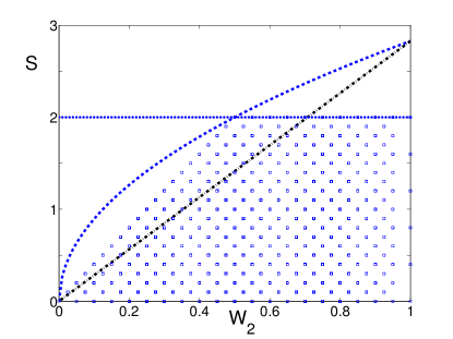
Figure 1: The Local Hidden Variable (LHV) and quantum predictions for $S$, for a given value of $W_{2}$ which is a measure of efficiency. The blue dashed curve is the Holder inequality bound, which provides an upper limit to the LHV prediction for $S$. The blue dotted line at $S=2$ is the CHSH inequality bound, which also provides an upper limit to the LHV prediction for $S$. The blue squares give a scattering of actual predictions for LHV theories. The observation of $S$ greater than either of the Holder or CHSH curves confirms the failure of all LHV theories. The dashed black solid line gives the quantum prediction, for the special case of a maximally entangled Bell state.

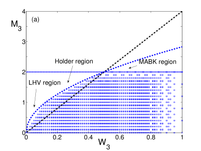
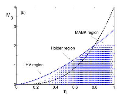
Figure 2: The Local Hidden Variable (LHV) and quantum predictions for $M_{3}$, versus efficiency. The top Figure plots $M_{3}$, for a specified value of $W_{N}$. The blue dashed curve is the Holder inequality bound, which gives an upper limit to the LHV predictions. The blue dotted line is the upper LHV bound given by the MABK inequality. The blue squares are a scattering of actual LHV predictions. The black line is the quantum prediction, for the maximally entangled GHZ state. The lower figure plots the predictions versus the actual efficiency at each site, for the case of symmetric detection efficiencies where $\eta_{k}=\eta$, $\forall k$.

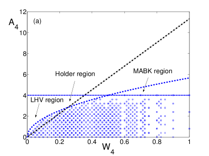
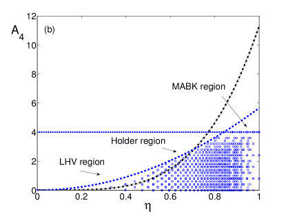
Figure 3: The LHV and quantum predictions for $Ar_{4}$ versus efficiency. The curves are as defined in Figures 1 and 2. The top figure gives the predictions for $Ar_{4}$, given a value of $W_{N}$. The lower figure gives the predictions for the special symmetric case, where $\eta_{k}=\eta$, $\forall k$. The blue curves are the Holder and MABK inequality bounds to the LHV predictions. The black line is the quantum prediction for a GHZ state.

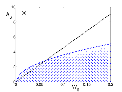
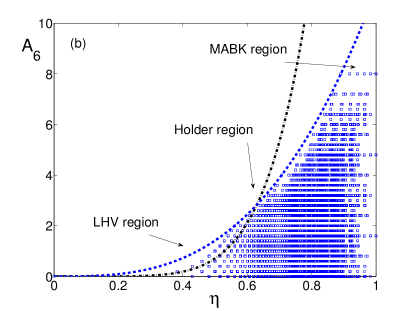
Figure 4: The LHV and quantum predictions for $Ar_{6}$ versus efficiency. The curves are as defined in Figures 1, 2 and 3. The top figure gives the predictions for $Ar_{6}$ for a given value of $W_{N}$. The lower figure gives the predictions for the special symmetric case, where $\eta_{k}=\eta$, $\forall k$. The blue curves are the Holder and MABK inequality upper bounds to the LHV predictions. The black line is the quantum prediction for a GHZ state. The Holder region is clearly apparent and in this region, we see that the Holder curve is a close fit to actual LHV predictions, indicated by the blue squares. The quantum prediction violates the LHV one, for $\eta$ approaching the limit of $0.5$, in this region.

More interesting behaviour is noticed for higher $N$. We identify three regions.

(1) MABK region: The figures show the region defined by $W_{N}>0.5$ (which corresponds to $\eta>0.5^{1/N}$ in the symmetric case where each $\eta_{k}=\eta$) and for which the LHV bound is that given by the MABK Bell inequalities. In this parameter range of $W_{N}$, which we call the “MABK region”, the Holder inequality bound is irrelevant. This region cannot be reached unless the efficiency at each site exceeds 50%: ie. $\eta_{k}>0.5$.

For $W_{N}<0.5$, we classify two regions.

(2) LHV region: This region is defined by $0<W_{N}<0.5^{N}$, which requires in the symmetric case, where all $\eta_{k}$ are equal, that the efficiency at each site is below $50\%$. This may be thought of as a “no-violation” or “LHV region” in that case, because of the simple result, that LHV theories cannot be violated using two-setting inequalities, if $\eta_{k}<0.5$ for each $k$. We outline an intuitive proof.

Proof: Suppose $N=2$, and that measurements at each site are made by observers Alice and Bob, respectively. Suppose also that losses are 50% at each of Alice’s and Bob’s channel. It is then possible that an “Eve” has tapped into Alice’s channel using a 50:50 beam splitter, and has created a second channel symmetric to Alice’s. Eve can make measurements on this second channel, simultaneously to Alice’s measurements. Alice can choose to measure either $A_{1}$ or $B_{1}$, and Eve can choose to measure either $A_{1}^{E}$ or $B_{1}^{E}$. In this case, by symmetry, we deduce that Eve’s measurements can have the same correlation with the measurements made by Bob as Alice’s measurements. A similar second Eve can exist at Bob’s channel, at site $k=2$. This second Eve can make measurements $A_{2}^{E}$, $B_{2}^{E}$. The potential existence of the two Eves necessarily downgrades the correlations of Alice and Bob, measured by $P(A_{1},A_{2})$, $P(B_{1},A_{2})$, $P(A_{1},B_{2})$ and $P(B_{1},B_{2})$, so that the probabilities cannot give a violation of the two-setting Bell inequality. This follows, since $A_{1}$, $A_{2}$, $B_{1}^{E}$ and $B_{2}^{E}$ can be measured simultaneously, and therefore there exists a joint probability distribution for those outcomes. The set $P(A_{1},A_{2})$, $P(B_{1}^{E},A_{2})$, $P(A_{1},B_{2}^{E})$ and $P(B_{1}^{E},B_{2}^{E})$ cannot therefore violate the Bell inequality. The symmetry of the correlations ($P(A_{1},B_{2})=P(A_{1},B_{2}^{E})$, etc) then allows us to deduce that there can be no violation of the Bell inequality for the measurements of Alice and Bob (since there exists an underlying probability distribution for these outcomes). The result is readily extended to higher $N$.

The proof depends on the existence of a symmetric beam splitter that creates, from one channel, $2$ symmetric channels, to give 50% loss on the first channel. The proof also utilises that the Bell inequality involves just two settings at each site, so that simultaneous measurements performed on two channels at each site can completely specify a joint probability distribution for the Bell inequality. An extension of the argument, assuming existence of a device that creates $m$ symmetric channels from $1$ channel, would lead to the conclusion that an $m$-setting Bell inequality cannot be violated where $\eta_{k}\leq 1/m$. Thus we deduce the requirement of $\eta_{k}>1/m$ for at least one $k$, for violation of an $m$-setting Bell inequality$\,\Diamond$.

The region $W<0.5^{N}$ is evident in the Figures as that corresponding to a straight-line relationship between actual LHV predictions and $W_{N}$. As expected, the quantum prediction is within the bound set by the LHV predictions.

(3) Holder region: The next region is the most interesting to us. This region shows a different LHV curve, closely approximated by the Holder analytic bound. We call this the “Holder” region. On examining the Figures, we find that, as $N$ increases above $2$, the quantum prediction moves from the MABK region ($W_{N}>0.5$) to intersect the LHV bound in the Holder region. This allows an analytic expression for the threshold efficiency in order to violate the two-setting Bell inequality:

$$\prod_{k=1}^{N}\eta_{k}>2^{(2-N)}$$ (17)

which corresponds to $\eta=0.79$ for $N=3$ and $\eta=0.5$ in limit of larger $N$, in the symmetric case $\eta_{k}=\eta$.

Our analysis thus establishes three new results. The main result is that the Holder expression gives a close fit to the LHV predictions, in this Holder region. This provides an analytical tool for understanding the LHV bounds in the two-setting scenario with loss. Second, we note that the quantum GHZ prediction intersects the Holder LHV bound, for all $N\geq 3$ even and odd, and moves “down” toward the edge of the “no-violation LHV” region as $N\rightarrow\infty$. The third new result is that violation of the two-setting Bell inequalities can be obtained without the requirement that each $\eta_{k}$ be greater than 50% (provided $N>3$). This is evident from the efficiency threshold (17). We see that if $N-1$ efficiencies are $1$, we only need an efficiency $\eta_{1}>4/2^{N}$ at the remaining site for a violation of the Bell inequality. This efficiency $\eta_{1}$ can be vanishingly small as $N\rightarrow\infty$.

VIII Discussion

The predicted efficiency thresholds do not quite match those shown to be possible by Cabello, Rodriguez and Villanueva cabello-1 for the case of odd $N$, but come very close (for $N=3$, $0.79$ versus $0.75$, for $N=5,$ $0.61$ versus $0.58$, for $N=7$). The difference is that CRV imposed an additional symmetric constraint on the LHV model, that each individual $\eta_{k}$ is measured and found precisely equal ($\eta_{k}=\eta$). This condition is practically reasonable, but is not imposed here. We have conditioned only on the value of $W_{N}$. Our case is informative, however, in revealing low efficiency thresholds in the asymmetric case, without the assumption of symmetric sites, and provides a rigorous way to test Bell nonlocality loophole-free, for practical realisations involving asymmetric transmission of entangled qubits.

The efficiency bounds deduced by Larsson and Semitecolos LS are even lower for a specified $N$, but are obtained using Clauser-Horne inequalities and nonmaximally entangled states. While CH inequalities are useful for loophole-free Bell tests CH ; cs , they rely on rarer joint detection events and thus is usually a less efficient use of the resource, particularly for larger $N$ parampNdemart . Understanding how to test loophole-free Bell nonlocality for the MABK situation and for maximally entangled GHZ states is therefore an important goal.

On that note, it is interesting to conjecture the usefulness of the Bell nonlocality that is realised in the two different regions, MABK and Holder. For many quantum information tasks, it is the genuine $N$-partite form of nonlocality that is the most useful ssgen . Genuine Bell nonlocality was considered by Svetlichny svet , and requires that the Bell nonlocality be truly shared among all $N$ sites, so that, for example, the system is not describable by the Bell nonlocality of a $k$-partite GHZ state, where $k<N$. The best known criterion for genuine Bell nonlocality is a violation of the Svetlichny inequality svet . This inequality reduces to $Ar_{N}\leq 2^{N-1}$ in our notation, and requires $W_{N}>\frac{1}{\sqrt{2}}$ ( $\eta>(\frac{1}{\sqrt{2}})^{1/N}$ for symmetric efficiencies) for violation, a violation that can only be obtained in the MABK region. We remark that any more general criterion for genuine Bell nonlocality will require, at least, that $\eta_{k}>0.5$ for each site. This remark is based on the result that Bell nonlocality will always imply a type of nonlocality called “steering” steer ; eprsteercav . From this knowledge, one may utilise results of Ref. eprsteer to establish the requirement of $\eta_{k}>0.5$ for each site. This requirement, however, does not necessarily imply the MABK region, and we leave as an open question whether genuine multipartite Bell nonlocality can be observed loophole-free in the Holder region.

IX Conclusion

In summary, we have established that the threshold efficiency for failure of local realism using GHZ states and the correlations of the two-setting MABK inequalities is $\prod_{k=1}^{N}\eta_{k}<0.5$, where $\eta_{k}$ is the efficiency at the $N$th site. This means that the maximally entangled GHZ state can indeed violate the predictions of LHV models, for symmetric efficiencies $\eta\rightarrow 0.5$ as $N\rightarrow\infty$. Furthermore, we have shown that for two-setting inequalities, there is no requirement (for loophole-free Bell tests) that the efficiency $\eta_{k}$ at each site exceed 50%, provided $N>3$.

The proposed experiment is very simple, and requires a measurement of efficiency only by measurement of the correlation $W_{N}$ which is readily evaluated from the spin results. While $\eta>0.5$ is a challenge for current experiments involving photons, the approach developed here may be extended to multi-setting Bell inequalities, for which the fundamental efficiency constraint is lower than $0.5$. The inequalities could be useful for detecting Bell nonlocality in future heralded experiments involving material particles, where loss is determined to be at a level somewhere between 0.5 and 1.

- (1) J. S. Bell, Physics 1, 195 (1964).
- (2) J. S. Bell, Foundations of Quantum Mechanics ed B d’Espagnat (New York: Academic) pp 171-81 (1971).
- (3) J. F. Clauser and A. Shimony, Rep. Prog. Phys. 41, 1881 (1978).
- (4) S. J. Freedman and J. F. Clauser, Phys. Rev. Lett. 28, 938 (1972).
- (5) A. Aspect, J. Dalibard, and G. Roger, Phys. Rev. Lett. 49, 1804 (1982).
- (6) G. Weihs, et al, Phys Rev. Lett. 81, 5039 (1998).
- (7) A. Peres, Phys. Rev. Lett. 77, 1413 (1996).
- (8) P. Pearle, Phys. Rev. D 2, 1418 (1970).
- (9) A Ekert, Phys. Rev. Lett. 67 661 (1991). V. Scarani and N. Gisin, Phys. Rev. Lett. 87, 117901 (2001). J. Barrett, L. Hardy and A. Kent, Phys. Rev. Lett. 95, 010503 (2005). A. Acin et al., Phys. Rev. Lett. 98, 230501 (2007).
- (10) J. F. Clauser, M. A. Horne, A. Shimony, and R. A. Holt, Phys. Rev. Lett. 23, 880 (1969).
- (11) N. D. Mermin, Phys. Rev. Lett. 65, 1838 (1990).
- (12) M. Ardehali, Phys. Rev. A, 46, 5375 (1992).
- (13) A. V. Belinskii and D. N. Klyshko, Physics-Uspekhi 36, 654, (1993). N. Gisin and H. Bechmann-Pasquinucci, Phys. Lett. A 246, 1 (1998).
- (14) A. Garg and N. D. Mermin Phys. Rev. D 35 3831 (1987).
- (15) J. F. Clauser and M. A. Horne, Phys. Rev. D 10, 526 (1974).
- (16) P. H. Eberhard, Phys. Rev. A 47 R747 (1993).
- (17) J. A. Larsson and J. Semitecolos, Phys Rev. A 63, 022117 (2001).
- (18) D. M. Greenberger, M. Horne, and A. Zeilinger, in Bell’s Theorem, Quantum Theory and Conceptions of the Universe, M. Kafatos, ed., (Kluwer, Dordrecht, The Netherlands) (1989).
- (19) S. L Braunstein and A. Mann, Phys. Rev. A 47, R2427, (1993). G. Brassard et al, Quantum Inf. Comput. 5, 538 (2005).
- (20) A. Cabello et al, Phys. Rev. Lett. 101, 120402 (2008).
- (21) A. Cabello and J. A. Larsson Phys. Rev. Lett. 98 220402 (2007).
- (22) N. Brunner, N. Gisin, V. Scarani, and C. Simon, Phys. Rev. Lett. 98, 220403 (2007).
- (23) E. G. Cavalcanti et al., Phys. Rev. Lett. 99, 210405 (2007).
- (24) Q. Y. He et al., Phys. Rev. A 81, 062106 (2010).
- (25) Q. Y. He et al., Phys. Rev. Lett. 103, 180402 (2009).
- (26) E. Schukin and W. Vogel, Phys. Rev. A 78, 032104 (2008).
- (27) A. Salles et al., Quant. Inf. Comput. 10, 0703-0719 (2010).
- (28) K-P. Marzlin and T. A. Osborn, arXiv: 1202.2534.
- (29) E. G. Cavalcanti et al, Phys. Rev. A 84, 0321158 (2011).
- (30) G. Svetlichny, Phys. Rev. D 35, 3066 (1987). D. Collins et al., Phys. Rev. Lett. 88, 170405 (2002).
- (31) G. Hardy, J. E. Littlewood and G. Polya, “Inequalities” (Cambridge University Press, London, 1934). M. Hillery, H. T. Dung and H. Zheng, Phys. Rev. A 81, 062322 (2010).
- (32) M. Zukowski et al., Phys. Rev. Lett. 88, 210402 (2002). X-H. Wu and H-S. Zong, Phys. Rev. 68, 032102 (2003). A W. Laskowski et al., Phys. Rev. Lett. 93, 200401 (2004).
- (33) R. F. Werner and M. M. Wolf, Phys. Rev. A 64, 032112 (2001).
- (34) S. Barz, G. Cronenberg, A. Zeilinger and P. Walther, Nature Photonics, 4, 553 (2010).
- (35) A. Fine, Phys. Rev. Lett. 48, 291 (1982).
- (36) M. D. Reid, W. Munro and F. de Martini, Phys. Rev. A 66, 033801 (2002).
- (37) M. Hillery et al., Phys. Rev. A 59, 1829 (1999).
- (38) H. M. Wiseman, S. J. Jones, and A. C. Doherty, Phys. Rev. Lett. 98, 140402 (2007). S. J. Jones et al., Phys. Rev. A 76, 052116 (2007).
- (39) E. G. Cavalcanti et al., Phys. Rev. A. 80, 032112 (2009).
- (40) Q. Y. He and M. D. Reid, arXiv: 1212.2270.